Inter-scale energy transfer in turbulence from the viewpoint of subfilter scales

1 Motivation and objectives

Understanding the cascading process of kinetic energy in turbulent flows from large-scale motions to smaller scales is critical in modeling strategies for geophysical and industrial flows. The phenomenological explanation of the transfer of energy across scales was conceptualized, first by Richardson (1922) and later by Obukhov (1941), as interactions among energy eddies of different sizes. The picture was completed in the classical paper by Kolmogorov (1941), and since then, many detailed investigations have greatly advanced our understanding of the energy cascade in high- Reynolds-number ($Re$) turbulent flows. Notwithstanding these efforts, the cascading process remains one of the most challenging problems in turbulence due to its non-linear and multiscale nature. In the present work, we investigate the inter-scale energy transfer (ISET) in turbulence from the viewpoint of subfilter scales (SFS). We show that this new perspective provides an amenable framework to characterize the energy transfer.

Attempts to unravel the mechanisms behind the cascade have relied on varying but complementary physical rationales. A classic explanation is given in terms of vortex stretching acting across scales (Leung et al., 2012; Goto et al., 2017; Lozano-Durán et al., 2016; Motoori & Goto, 2019). Other approaches have directly tested Richardson’s idea in terms of eddy breakdown (Lozano-Durán & Jiménez, 2014b), or energy transfer among eddies at different scales (Cardesa et al., 2017). The advent of multifractal representations of the cascade (Meneveau, 1991; Frisch & Vergassola, 1991; Frisch & Donnelly, 1996; Mandelbrot, 1999; Jiménez, 2000; Yang & Lozano-Durán, 2017) and wavelet methods (Farge, 1992; Schneider & Vasilyev, 2010) have also opened new avenues for analyzing the statistical properties of the energy transfer across scales.

A distinction should be made between the different approaches discussed above in terms of (i) tools, which may include wavelets (Meneveau, 1991), coherent structures (Lozano-Durán & Jiménez, 2014b), space-time correlations (Wan et al., 2010), filtering of the equations (Piomelli et al., 1991), and so forth, and (ii) quantities, which may include source/sink terms in the energy (Aoyama et al., 2005) or the enstrophy (Leung et al., 2012; Lozano-Durán et al., 2016) equation, vortex stretching and strain self-amplification (Betchov, 1956; Tsinober, 2009), the kinetic energy itself (Cardesa et al., 2017), and so on. What may appear as a purely semantic debate is in fact an attempt to tackle the problem of how to look at the energy cascade. Here, we are concerned with choosing the most appropriate quantity to characterize the energy cascade, since tools only differ in how they handle this quantity.

The starting point for many studies of the energy cascade is the decomposition of the flow into resolved and unresolved (or subfilter) scales, inherent to high-$Re$ turbulence. This partition of the flow has been extensively used both for physical understanding of the energy cascade and for its reduced-order modeling. In the latter, accurate predictions of the flow require a faithful interpretation of the subfilter physics and of its interaction with the resolved field. In this context, a set of ubiquitous terms are given by the SFS stresses,

$$\tau_{ij}=\overline{u_{i}u_{j}}-\overline{u}_{i}\overline{u}_{j},$$ (1)

appearing in the filtered momentum equations, written here in incompressible form

$$\partial_{t}\overline{u}_{i}+\overline{u}_{j}\partial_{j}\overline{u}_{i}=-\partial_{i}\overline{p}-\partial_{j}\tau_{ij}+\nu\partial_{j}\partial_{j}\overline{u}_{i}+\overline{F}_{i}.$$ (2)

We follow the convention of decomposing the total velocity $u_{i}$ into $u_{i}=\overline{u}_{i}+u^{\prime}_{i}$, where

$$\overline{u}_{i}\left(\boldsymbol{x}\right)=\int u_{i}\left(\boldsymbol{x}-\boldsymbol{r}\right)G\left(\boldsymbol{r}\right)\mathrm{d}\boldsymbol{r}$$ (3)

is the resolved velocity defined with respect to some filter $G(\boldsymbol{r})$. The spatial Cartesian coordinates are $\boldsymbol{x}\equiv(x_{1},x_{2},x_{3})$ (and occasionally $\boldsymbol{x}\equiv(x,y,z)$), $F_{i}$ is a forcing term, and $\overline{F}_{i}$ is its filtered counterpart. The kinematic viscosity of the flow is $\nu$, and the pressure scaled by a constant density is $p$. The term $P=\overline{S}_{ij}\tau_{ij}$ is the ISET, and it appears with opposite sign in the evolution equations of two energy definitions: $\overline{u}_{i}\overline{u}_{i}$ and $\tau_{ii}$.

To model $\partial_{j}\tau_{ij}$ in Eq. (2), it is essential that $P$ be consistent with phenomenological aspects of the energy cascade. As a result, modelers are often concerned with the properties of $P$ when feeding physics into their large-eddy simulation (LES) models. We argue, however, that studying the physics of the energy cascade through term $P$ can be significantly improved upon. We describe the issues associated with the use of $P$ as a marker for ISET, and propose an alternative ISET term more suitable to study the spatial structure of energy transfer across scales.

This brief is organized as follows. In Section 2 we introduce the filter-scale energy equations, discuss the properties of the sources and sinks of kinetic energy, and identify our target features concerning an optimal ISET term. A similar analysis is performed in Section 3 for the kinetic energy associated with the subfilter velocities, and a new energy transfer term $T$ is introduced. Comparisons between $T$ and $P$ for different flows and for various filters are offered in Section 4 and Section 5. Finally, we present our conclusions in Section 6.

2 Equations for the filter-scale kinetic energy

2.1 Subfilter-scale energy transfer and alternative formulations

The traditional ISET term $P$ is found in the equation for the kinetic energy of the filtered velocities,

$$\left(\partial_{t}+\overline{u}_{j}\partial_{j}\right)\frac{1}{2}\overline{u}_{i}\overline{u}_{i} =-\partial_{j}\left(\overline{u}_{j}\overline{p}+\overline{u}_{i}\tau_{ij}-2\nu\overline{u}_{i}\overline{S}_{ij}\right)-2\nu\overline{S}_{ij}\overline{S}_{ij}+\underbrace{\overline{S}_{ij}\tau_{ij}}+\overline{u}_{i}\overline{F}_{i}.$$

$$\hskip 162.18062ptP$$

$P$ is commonly interpreted as the rate of transfer of kinetic energy from the filtered motions to the residual motions (Pope, 2000), i.e., energy transport in scale. The frequent justification for this meaning stems from the fact that $P$ is outside the divergence, so that it cannot be energy transport in space. While there is evidence and agreement that, for a given flow field, the spatial distribution and statistical properties of $P$ depend heavily on the filter used (Piomelli et al., 1991; Aoyama et al., 2005; Cardesa et al., 2015), it is less commonly acknowledged that there are alternative formulations of Eq. (2.1). In alternative formulations, the resulting term outside the divergence could be assigned the same interpretation as that of $P$, since whatever is outside of the divergence (and is non-viscous) should be transport in scale. For instance,

$$\left(\partial_{t}+\overline{u}_{j}\partial_{j}\right)\frac{1}{2}\overline{u}_{i}\overline{u}_{i} =-\partial_{j}\left(\overline{u}_{j}\overline{p}-2\nu\overline{u}_{i}\overline{S}_{ij}\right)-2\nu\overline{S}_{ij}\overline{S}_{ij}+\underbrace{\overline{u}_{i}\partial_{j}\left(\tau_{ij}\right)}+\overline{u}_{i}\overline{F}_{i}.$$

$$\hskip 130.88284ptP_{2}$$

$P_{2}$ and $P$ have the same spatially averaged value in the absence of boundary fluxes, yet their pointwise values differs significantly. Since LES models benefit from information on the physics of what occurs at each grid point, arguing that $P_{2}$ and $P$ only differ by an amount that cancels out on the average does not settle an important issue: what is the pointwise ISET of the flow? The question is central to LES models that attempt to handle the presence of the so-called backscatter, which is a local property of $P$ (Piomelli et al., 1991; Cerutti & Meneveau, 1998). The question also highlights the need for refined criteria when assigning a meaning to a term in an equation.

Another concerning aspect of $P$ in Eq. (2.1) is that the term $\overline{u}_{i}\tau_{ij}$ inside the divergence of Eq. (2.1) can be expanded as

$$\overline{u}_{i}\tau_{ij}=\overline{u}_{i}\left(\overline{\overline{u}_{i}\overline{u}_{j}}+\overline{\overline{u}_{i}u^{\prime}_{j}}+\overline{\overline{u}_{j}u^{\prime}_{i}}+\overline{u^{\prime}_{i}u^{\prime}_{j}}-\overline{u}_{i}\overline{u}_{j}\right).$$ (6)

The terms in parentheses include both filter-scale and SFS interactions, so that a product of $\tau_{ij}$ with $\overline{u}_{i}$ involves inter-scale coupling by necessity. Hence, $P$ does not contain all coupling between filter scales and SFS in the right-hand side of Eq. (2.1). In view of these observations, it is difficult to assign to $P$ the role of causing all energy changes stemming from filter-subfilter interactions. This illustrates the challenge of trying to distinguish between terms transporting energy entirely in space or purely across scales.

2.2 Galilean invariance

An additional consideration is that of Galilean invariance. Briefly, the Galilean transformation is defined as

$$\hat{x}_{i}=x_{i}-V_{i}t;\hskip 28.45274pt\hat{t}=t;\hskip 28.45274pt\hat{u}_{i}=u_{i}-V_{i},$$ (7)

where $V_{i}$ is the constant velocity of the frame of reference. We provide in the Appendix some identities related to Eq. (7) used on filtered and residual velocity components. Applying the transformations to the momentum equations, we find that the rate of change on the left-hand side preserves both its form and its value under Galilean transformations,

$$\left(\partial_{t}+u_{j}\partial_{j}\right)u_{i}=\left[\hat{\partial}_{t}-V_{j}\hat{\partial}_{j}+\left(\hat{u}_{j}+V_{j}\right)\hat{\partial}_{j}\right]\left(\hat{u}_{i}+V_{i}\right)=\left(\hat{\partial}_{t}+\hat{u}_{j}\hat{\partial}_{j}\right)\hat{u}_{i}.$$ (8)

The same applies to the filtered momentum equations.

The situation contrasts starkly with the transformed kinetic energy equation. Applying the transformations to Eqs. (2.1) and (2.1), we find that the left-hand side becomes

$$\left(\partial_{t}+\overline{u}_{j}\partial_{j}\right)\frac{1}{2}\overline{u}_{i}\overline{u}_{i}=V_{i}\left(\hat{\partial}_{t}+\overline{\hat{u}}_{j}\hat{\partial}_{j}\right)\overline{\hat{u}}_{i}+\left(\hat{\partial}_{t}+\overline{\hat{u}}_{j}\hat{\partial}_{j}\right)\frac{1}{2}\overline{\hat{u}}_{i}\overline{\hat{u}}_{i}.$$ (9)

In the first term of the right-hand side of Eq. (9), $V_{i}$ multiplies the left-hand side of the (filtered) momentum equations. This term cancels out with an equivalent term on the right-hand side of the transformed Eq. (2.1) or Eq. (2.1), so that overall, Eqs. (2.1) and (2.1) preserve their form and are thus Galilean invariant. However, the rates of change of energy observed on different Galilean frames of reference will differ in value, even if the law those changes obey appears to be the same.

To illustrate the difference, we present the following thought experiment. Let the rate of change $(\partial_{t}+\overline{u}_{j}\partial_{j})\overline{u}_{i}\overline{u}_{i}/2$ at a given point and instant be $q$ on the static frame of reference. Then, according to Eq. (9), it is possible to choose a $V_{i}$ such that the first term on the right-hand side of Eq. (9) equals $q$. In that Galilean frame of reference, the rate of change of energy given by the last term in Eq. (9) would be zero.

The argument above shows how a Galilean-invariant equation needs not lead to rates of change which are themselves Galilean invariant. In addition, individual terms in a Galilean-invariant equation need not be Galilean invariant. For example, it is straightforward to prove that $P$ is Galilean invariant while $P_{2}$ is not, yet both appear in Galilean-invariant equations. Hence, $P$ is a better ISET term candidate than $P_{2}$ in terms of independence from the frame of reference.

The implications of the discussion above lead us to conclude that a preliminary step in choosing a suitable form of the ISET term is the choice of the appropriate equation. Indeed, it is desirable to study the terms in an equation which preserves identical rates of change on different Galilean frames of reference, as is the case for the momentum equation. We also seek, if possible, an equation where terms are individually Galilean invariant. A drawback of not doing so appears when looking at the pointwise value of individual terms. If the latter are not Galilean invariant term by term, then the relative importance of, say, a divergence term compared to an ISET term will depend on the frame of reference, which is unsatisfactory from a fundamental point of view — even though the sum of all terms on both sides of the equation balances out. The considerations regarding Galilean invariance of individual terms are similar to those concerning improved expressions for the SFS stress models (Speziale, 1985; Germano, 1986) discussed in the past.

3 Equations for the subfilter-scale kinetic energy

It was argued above that studying the kinetic energy transfer from the point of view of the filter scales entails a series of drawbacks which are intrinsic to the formulation of the equation itself. Several prerequisites are identified in the previous section concerning the target ISET term. We summarize them below. In essence, we are aiming to obtain an ISET term that:

1. belongs to an equation that conserves the value of the rate of change of energy under Galilean transformations,

2. belongs to the right-hand side of an equation where each product is individually Galilean invariant,

3. avoids filter-subfilter coupling inside the spatial flux term, and

4. avoids filter-only or subfilter-only coupling.

The decomposition between filter scales and SFS has triggered the consideration of several kinetic energy expressions. One of the most extended list of expressions is perhaps that presented in Section 3.3.1 of Sagaut (2006). Nonetheless, little or no consideration has been paid to the evolution equation for the kinetic energy of the subfilter velocities. It can be shown that the equation for the kinetic energy of the subfilter (residual) scales preserves the value of the rate of change under Galilean transformations. Various equations can be derived depending on the particular arrangement of terms on the right-hand side,

$$\left(\partial_{t}+\overline{u}_{j}\partial_{j}\right)\frac{1}{2}u^{\prime}_{i}u^{\prime}_{i} = -\partial_{j}\left(u^{\prime}_{j}p^{\prime}-2\nu u^{\prime}_{i}S^{\prime}_{ij}\right)-2\nu S^{\prime}_{ij}S^{\prime}_{ij}$$ (10)

$$+ \underbrace{u^{\prime}_{i}\partial_{j}\left(\tau_{ij}\right)-u^{\prime}_{i}u^{\prime}_{j}\overline{S}_{ij}-u^{\prime}_{i}u^{\prime}_{j}S^{\prime}_{ij}}_{T_{a}}+u^{\prime}_{i}F^{\prime}_{i}$$

$$\left(\partial_{t}+\overline{u}_{j}\partial_{j}\right)\frac{1}{2}u^{\prime}_{i}u^{\prime}_{i} = -\partial_{j}\left(u^{\prime}_{j}p^{\prime}-2\nu u^{\prime}_{i}S^{\prime}_{ij}-u^{\prime}_{i}\tau_{ij}\right)-2\nu S^{\prime}_{ij}S^{\prime}_{ij}$$ (11)

$$+ \underbrace{-S^{\prime}_{ij}\tau_{ij}-u^{\prime}_{i}u^{\prime}_{j}\overline{S}_{ij}-u^{\prime}_{i}u^{\prime}_{j}S^{\prime}_{ij}}_{T_{b}}+u^{\prime}_{i}F^{\prime}_{i}$$

$$\left(\partial_{t}+\overline{u}_{j}\partial_{j}\right)\frac{1}{2}u^{\prime}_{i}u^{\prime}_{i} = -\partial_{j}\left(u^{\prime}_{j}p^{\prime}-2\nu u^{\prime}_{i}S^{\prime}_{ij}+\frac{1}{2}u^{\prime}_{i}u^{\prime}_{i}u^{\prime}_{j}\right)-2\nu S^{\prime}_{ij}S^{\prime}_{ij}$$ (12)

$$+ \underbrace{u^{\prime}_{i}\partial_{j}\left(\tau_{ij}\right)-u^{\prime}_{i}u^{\prime}_{j}\overline{S}_{ij}}_{T_{c}}+u^{\prime}_{i}F^{\prime}_{i}$$

$$\left(\partial_{t}+\overline{u}_{j}\partial_{j}\right)\frac{1}{2}u^{\prime}_{i}u^{\prime}_{i} = -\partial_{j}\left(u^{\prime}_{j}p^{\prime}-2\nu u^{\prime}_{i}S^{\prime}_{ij}-u^{\prime}_{i}\tau_{ij}+\frac{1}{2}u^{\prime}_{i}u^{\prime}_{i}u^{\prime}_{j}\right)-2\nu S^{\prime}_{ij}S^{\prime}_{ij}$$ (13)

$$+ \underbrace{S^{\prime}_{ij}\tau_{ij}-u^{\prime}_{i}u^{\prime}_{j}\overline{S}_{ij}}_{T_{d}}+u^{\prime}_{i}F^{\prime}_{i}.$$

As stated previously, the motivation for looking at these equations is that the left-hand side complies with prerequisite a), which Eq. (2.1) fails to do. The term $\overline{u}_{i}\partial_{j}(u^{\prime}_{i}u^{\prime}_{j})$ appears in alternative ways of writing the right-hand side of Eqs. (10)–(13), which is inconsistent with b), so we do not consider those expressions. Visual inspection of Eqs. (11) and (13) reveals that some filter-subfilter coupling remains inside the divergence through the $u^{\prime}_{ij}\tau_{ij}$ term, which goes against c). Choosing between Eqs. (10) and (12) relies on compliance with d), which Eq. (12) achieves to a larger extent by avoiding the presence of $u^{\prime}_{i}u^{\prime}_{j}S^{\prime}_{ij}$ inside the ISET term. Expanding $\tau_{ij}$ within $T_{c}$, we find the product $u^{\prime}_{i}\partial_{j}\overline{u^{\prime}_{i}u^{\prime}_{j}}$. While its interpretation as a subfilter-only term is arguable, it appears in the equation which comes closest to complying with all four established prerequisites, and therefore we choose $T_{c}$ as our ISET term and relabel it as

$$T=u^{\prime}_{i}\partial_{j}\left(\tau_{ij}\right)-u^{\prime}_{i}u^{\prime}_{j}\overline{S}_{ij}.$$ (14)

When comparing Eqs. (12) and (2.1), one should not forget that

$$u_{i}u_{i}=\overline{u}_{i}\overline{u}_{i}+2\overline{u}_{i}u^{\prime}_{i}+u^{\prime}_{i}u^{\prime}_{i}.$$ (15)

There are thus a wealth of additional energy equations related to the evolution of $\overline{u}_{i}u^{\prime}_{i}$, which invariably fail to comply with a). It is tempting to assume that, by construction, we have removed any dependence on the large scales of the flow by looking at the evolution of $u^{\prime}_{i}u^{\prime}_{i}$ instead of $\overline{u}_{i}u^{\prime}_{i}$ or $\overline{u}_{i}\overline{u}_{i}$. It is not so, however, since the evolution equations considered above relate to rates of change as perceived by an observer traveling with velocity $\overline{u}_{j}$, which preserves the large-scale information. In addition, the energy gained or lost through $T$ invetably comes from or goes to the large scales, so in principle there is no reason to believe we are enforcing a removal of large-scale dependence.

Some statistical properties of terms $T_{a}$, $T_{b}$, $T_{c}$, and $T_{d}$ were studied by Cardesa & Jiménez (2016) for one flow, confirming that $T_{c}$ featured the most desirable properties of all four candidates in terms of acting as the small-scale counterpart of $P$. In the next section, we compare the views of ISET obtained through $T$ and $P$ for several flows. Before doing so, we note in passing that compliance with a) would also hold for the evolution equation of $\tau_{ii}$. However, we discard that equation for failing to comply with b) and c), as detailed in the Appendix.

4 Comparison between $T$ and $P$ for different flows

We compute $T$ and $P$ in three different flows obtained by direct numerical simulation (DNS), namely, homogeneous shear turbulence (HST), homogeneous isotropic turbulence (HIT), and a plane turbulent channel flow (CH4K). The details of the three simulations can be found in Table 1. The large scales of the three flows selected differ significantly from one another, so that we can benchmark the degree of dependence of $T$ and $P$ on the large scales.

All three flows have been filtered with an isotropic low-pass Gaussian filter defined as

$$\tilde{G}(\boldsymbol{k})=\exp\left[-\left(r\boldsymbol{k}\right)^{2}/40\right]$$ (16)

in Fourier space, where $\boldsymbol{k}$ is the wave number and $r$ is the filter width. The filtering was applied to the Fourier modes of the velocity components of HIT, as well as in the streamwise and spanwise directions of HST and CH4K. In HST, filtering along $y$ was implemented by convolving the velocity with the real-space transform of $G\left(y\right)=f\exp[-6y^{2}/r^{2}]$, where $f$ is a constant chosen to meet the normalization condition. In CH4K, the filtering in the wall-normal direction was carried out following the procedure described by Lozano-Durán et al. (2016). We used only values of $T$ and $P$ extracted from the plane at the channel centerline, where the flow inhomogeneity is the weakest. The width of the largest filter used is $672\eta$, where $\eta$ is the Kolmogorov length scale based on the dissipation at the channel centerline. The wall-to-wall distance is $1062\eta$, and the widest filter extends from the centerline down to $y/h=0.37$ or $y^{+}=1533$ from both walls. This is close to the edge of the log-law region (Lozano-Durán & Jiménez, 2014a), so that most filter widths characterize essentially the core of the channel.

Case	$Re_{\lambda}$	$N_{x}\times N_{y}\times N_{z}$	$(L_{x}\times L_{y}\times L_{z})/\eta$	$L_{o}/\eta$
HST	107	$768\times 512\times 255$	$1117\times 745\times 372$	267
CH4K	161	$2048\times 541\times 2047$	$3337\times 1062\times 1668$	1397
HIT	236	$512^{3}$	$1011^{3}$	876

Table 1: Details of the three simulations used: homogeneous shear turbulence (HST), a plane channel flow at friction-based Reynolds number $Re_{\tau}=4179$ (CH4K), and homogeneous isotropic turbulence (HIT). All flows are incompressible and statistically steady. $N_{i}$ and $L_{i}$ are the number of degrees of freedom and the domain size in directions $i=x,y,$ and $z$, which for the shear flows HST and CH4K correspond to streamwise, vertical, and spanwise directions, respectively. The Kolmogorov length scale $\eta$ is given by $(\nu^{3}/\epsilon)^{1/4}$, where $\nu$ is the kinematic viscosity and $\epsilon$ the mean rate of kinetic energy dissipation. For CH4K, $\eta$ is that measured at the channel centerline. For HST and CH4K, the Reynolds number based on the Taylor microscale is defined as $Re_{\lambda}=K^{2}[5/(3\nu\epsilon)]^{1/2}$, where $K^{2}$ is twice the kinetic energy of the velocity field fluctuating with respect to the time-averaged, $y$-dependent streamwise mean velocity. For HIT, $Re_{\lambda}$ is computed in the standard way, while $K^{2}$ is twice the total kinetic energy. $L_{o}=K^{3}/\epsilon$ is a length scale characterizing the large scales. For more details on the simulations, CH4K is case M4200 in Lozano-Durán & Jiménez (2014a), while HST and HIT are documented by Cardesa et al. (2015).

4.1 Net amount of forward and backward energy cascade

The ratio between the volumes of flow experiencing forward to backward ISET is shown in Figure 1(a). The spatial predominance of the forward cascade is perceived through both ISET terms $T$ and $P$. Ratios based on $T$ are lower than for $P$, except for the narrow filter widths in the viscous range, where they converge to similar values. The most striking difference between the picture of the cascade obtained with both ISET terms is that ratios based on $P$ exhibit a stronger $r$ dependence than those based on $T$. It is best illustrated by the drop at large $r$ in the ratio of the CH4K case when based on $P$ and not on $T$. In addition, the ratio in the HST case differs significantly from the other two flows for larger $r$ when computed with $P$ and not so with $T$. The largest filter width in the HST case is $227\eta$, which is perhaps close enough to the spanwise extent of the box ($372\eta$) to have an impact on the statistics. But whatever the reason for the divergence from the other two flows, the ratio for HST based on $T$ is not impacted, while that based on $P$ is. It appears that $T$ filters out differences across flows and across $r$, providing a more homogeneous view of the cascade. Very similar conclusions are reached by looking at the ratios of forward to backward ISET in terms of actual energy flux in Figure 1(b). The main difference between Figure 1(a) and Figure 1(b) is that the ratios of forward to backward cascade are higher when quantified with the energy fluxes rather than with flow volumes, and this is clear for both $T$ and $P$.

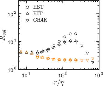
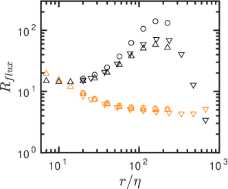
(a)                                                 (b)

Figure 1: Ratios of direct (forward) over inverse (backward) cascade based on $T$ (orange) and $P$ (black). For $T$, forward and backward cascade correspond to $T>0$ and $T<0$, respectively. $P<0$ and $P>0$ are taken as forward and backward cascade, respectively. (a) (flow volume forward) / (flow volume backward), (b) (energy flux forward) / (energy flux backward).

4.2 Structure of forward/backward-cascading transfer eddies

We now focus on case HIT and study the properties of the scalar field $T>\alpha^{+}$, where $\alpha^{+}>0$ is a thresholding parameter. For each $r$, we select a value of $\alpha^{+}$ such that the rate of change of the total volume enclosed by $T>\alpha^{+}$ decreases most with increasing threshold (see the percolation theory by Kesten, 1982). We repeat the process for the field $T<\alpha^{-}$ with $\alpha^{-}<0$. The resulting structures of intense $|T|$ (collectively denoting $T>\alpha^{+}$ and $T<\alpha^{-}$) are plotted in Figure 2(a) for $r=14\eta$ and in Figure 2(c) for $r=160\eta$. The same steps are followed for $P$, shown in Figures 2(b,d). The visualizations reveal that $|T|$ and $|P|$ structures obtained for $r=14\eta$ bear clear similarities, while those obtained for $r=160\eta$ do not. This is in agreement with the fact that, in Figure 1, the disparity between the cascade ratios computed for $T$ and $P$ is considerably smaller for filter widths within the viscous range than for filter widths above $100\eta$. Furthermore, by comparing the structures of intense $|T|$ at $r=14\eta$ and $r=160\eta$, one is able to observe similarities between Figures 2(a,c), consistent with the similar events that have simply grown in scale. It is challenging, however, to see any similarities between Figures 2(b) and 2(d), so that the picture that emerges through $P$ is extremely dependent upon the filter width $r$ — at least, much more so than upon $T$. Again, this is consistent with Figure 1, in which cascade ratios based on $T$ are significantly less $r$ dependent than those based on $P$.

The probability density function (PDF) of $P$ is known to be negatively skewed and to depend on scale and filter type (Piomelli et al., 1991; Aoyama et al., 2005). The PDF of $T$ has not been documented, and it is reported here along with that of $P$ (Figure 3). The skewness of $T$ is of opposite sign to that of $P$, which is perhaps unsurprising since one expects extreme negative $P$ events to have an extreme positive $T$ counterpart. What is remarkable in our view concerns the tails of the PDFs in the backscatter region — i.e., $P>0$ and $T<0$. While the tails of $P$ for large $r$ suffer a drastic change, also observed by Aoyama et al. (2005), the tails in the $T<0$ side are less affected by the changes in $r$, providing a rather different view of backscatter than that obtained through $P$. The stronger $r$ dependence of the shape of the PDFs of $P$ compared to those of $T$ explains the major departure of the aspect of the flow structures observed in Figure 2(d) from those in Figure 2(a-c).

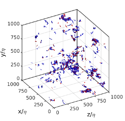
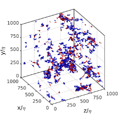
(a)                                                 (b)

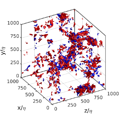
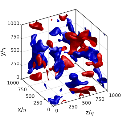
(c)                                                 (d)

Figure 2: Case HIT: objects of intense $|T|$ (left) and intense $|P|$ (right). (a) and (b): $r=14\eta$. (c) and (d): $r=160\eta$. Red objects contain forward cascade ($P<0$ or $T>0$), blue objects contain backward cascade ($P>0$ or $T<0$).

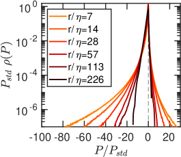
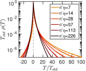
(a)                                                 (b)

Figure 3: Probability density function $\rho$ of $P$ (a) and $T$ (b), normalized by the respective standard deviations $P_{std}$ and $T_{std}$. Case HIT.

5 Comparison between $T$ and $P$ for different filter shapes

We now focus on a single flow and test different filter definitions. Taking case HIT, we filter the velocity field following three filters defined in Fourier space as

$$\text{Gaussian:}\hskip 28.45274pt\tilde{G}(\boldsymbol{k}) = \exp\left[-\left(r\boldsymbol{k}\right)^{2}/40\right],$$ (17)

$$\text{Top-hat:}\hskip 28.45274pt\tilde{G}(\boldsymbol{k}) = 3\left[\sin\left(\zeta\right)-\zeta\cos\left(\zeta\right)\right]/\zeta^{3},$$ (18)

$$\text{Cutoff:}\hskip 28.45274pt\tilde{G}(\boldsymbol{k}) = H\left(\frac{\pi}{r}-|\boldsymbol{k}|\right),$$ (19)

where $\zeta=|\boldsymbol{k}|r/2$ and $H$ is the Heaviside step function. These definitions are adjusted so that the Gaussian and top-hat filters have matched second moments (Borue & Orszag, 1998). It is practical to repeat Eq. (16) here with Eq. (17) for the sake of clarity. While the cutoff filter is sharp in spectral space and oscillates in real space, the top-hat has the opposite behavior with a sharp behavior in real space and oscillations in Fourier space. The Gaussian filter is free from oscillations in both spaces.

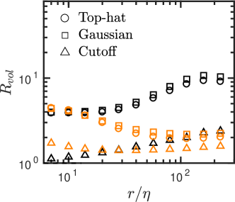
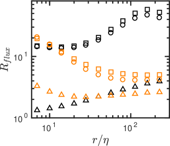
(a)                                                 (b)

Figure 4: Ratios of direct (forward) to inverse (backward) cascade based on $T$ (orange) and $P$ (black). For $T$, forward and backward cascade correspond to $T>0$ and $T<0$, respectively. $P<0$ and $P>0$ are taken as forward and backward cascade, respectively. Case HIT. (a) (flow volume forward) / (flow volume backward). (b) (energy flux forward) / (energy flux backward).

The ratios of forward to backward cascade based on volume fractions and on energy fluxes are shown in Figure 4. For a given ISET term, the ratios based on the top-hat and Gaussian filters are in good agreement with each other. The cutoff filter gives a different set of ratios regardless of ISET term. The two filters that do not oscillate in real space show cascade ratios which compare well across ISET terms for the low-end range of $r$ values, but disagreement between $T$- and $P$-based ratios grows for larger filter widths. For $r$ larger than the viscous-dominated scales, the ratios based on $T$ vary less with filter type than those based on $P$, with the cutoff filter showing similar ratios to the other two filters for $T$-based ratios and not so for $P$-based ratios.

The impact of the filter type on the PDFs at three different scales is illustrated in Figure 5. The PDFs on the right of Figure 5 show that $T$ has distributions based on the cutoff filter which significantly differ from those obtained with the other two filters. However, the impact of the cutoff filter on the PDFs of $P$ is even more striking at all three values of $r$ considered.

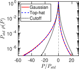
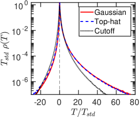
(a)                                                 (b)

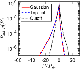
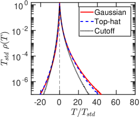
(c)                                                 (d)

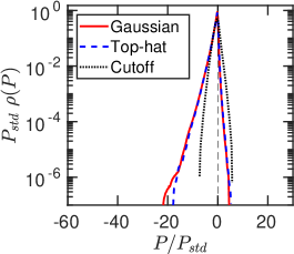
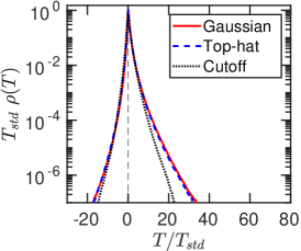
(e)                                                 (f)

Figure 5: Probability density function $\rho$ of $P$ (left) and $T$ (right) for the three different filters defined in Eqs. (17)-(19), normalized by the respective standard deviations $T_{std}$ and $P_{std}$. Case HIT. (a) and (b): $r=20\eta$. (c) and (d): $r=80\eta$. (e) and (f): $r=160\eta$.

6 Conclusions

The average transfer of kinetic energy from large to small flow motions has been the cornerstone of most theories and models of the turbulence cascade since the 1940s. Yet predicting the spatial structure of the kinetic energy transfer by going beyond the average tendency and tackling the point-to-point description remains an outstanding challenge in fluid mechanics. Despite the broad knowledge acquired in recent years, advances in the characterization of the energy cascade have been hampered by the ambiguity and disparity in the tools and quantities to be considered.

Very often, the energy cascade has been studied via the filtered equations of motion leading to the term $P=\tau_{ij}\overline{S}_{ij}$ as the main figure of merit. Here, we have highlighted that the particular choice of $P$ is, to some extent, arbitrary and that alternative definitions of ISET are possible while still preserving the same physical meaning ascribed to $P$. We have argued that distinct ISET terms appear depending on the arrangement of the right-hand side of the filtered kinetic energy equation. We have illustrated this using as an example the term $P_{2}=\overline{u}_{i}\partial_{j}\tau_{ij}$.

However, while alternative formulations of $P$ exist, they do not comply with our requirements for a physically sound ISET term. The deficiencies can be traced back to i) the Galilean invariance of the rate of energy change as a whole, ii) the Galilean invariance of ISET and other terms in an equation, and iii) the remaining filter-subfilter coupling inside the spatial transport term leading to erroneous interpretations as energy flux in space. We have shown that $P$, despite its Galilean invariance, is within an equation where the total rate of energy change depends on the inertial frame of reference and filter-subfilter coupling is contained in the spatial transport part of Eq. (2.1). $P_{2}$ lacks Galilean invariance.

To address the shortcomings exposed above, we have proposed to study the energy cascade from the point of view of the SFS kinetic energy equation. We have shown that, by a judicious arrangement of the terms in the equations, it is possible to formulate an ISET term which i) belongs to an equation that conserves the value of the rate of change of energy under Galilean transformations, ii) is composed of terms that are all individually Galilean invariant, and iii) leaves no remaining filter-subfilter coupling inside the spatial transport term. This new term is given by $T=u^{\prime}_{i}\partial_{j}\left(\tau_{ij}\right)-u^{\prime}_{i}u^{\prime}_{j}\overline{S}_{ij}$.

We have studied the properties of $T$ and $P$ as markers to describe the energy cascade. To that end, we analyzed data from DNS of three flow configurations: HST, HIT, and turbulent channel flow. The ratios of forward to backward cascade based on $T$ are roughly independent of the flow despite the very different large scales. This contrasts with ratios based on $P$, which exhibit strong flow and filter width dependence. The statistical properties of $T$, such as the amount of forward cascade and backscatter, show milder dependence on the filter type than those of $P$, at least within the range of filter types considered here. In conclusion, our results suggest that $T$ portrays a picture of the energy cascade that is much closer to self-similar and universal across flows and for a wider range of scales, in contrast to the picture provided by the traditional $P$.

The present study is centered about improvements in the physical understanding of the turbulent cascade rather than in practical model implementation. We leave for future studies the connection between $T$ and improved SFS models for LES.

Appendix A. Galilean invariance of filtered velocities

The filter function $G$ in Eq. (3) satisfies the normalization condition

$$\int G(r_{i})dr_{i}=1.$$ (A.1)

The Galilean transformation applied to the filtered velocity yields

$$\overline{u}_{i}=\int u_{i}(x_{j}-r_{j})G(r_{j})dr_{j}=\int\hat{u}_{i}(x_{j}-r_{j})G(r_{j})dr_{j}+\int V_{i}G(r_{j})dr_{j},$$

$$=\int\hat{u}_{i}(x_{j}-r_{j})G(r_{j})dr_{j}+V_{i}\int G(r_{j})dr_{j}=\overline{\hat{u}}_{i}+V_{i},$$ (A.2)

so that the filtered velocity depends on the frame velocity $V_{i}$. For this reason, the terms $P_{2}$ in Eq. (2.1) and $\overline{u}_{i}\partial_{j}(u^{\prime}_{i}u^{\prime}_{j})$, which appear in alternative ways of writing the right-hand side of Eqs. (10) and (13), are not Galilean invariant. On the contrary, the residual velocity $u^{\prime}_{i}$ is given by

$$u^{\prime}_{i}=u_{i}-\overline{u}_{i}=\hat{u}_{i}+V_{i}-\overline{u}_{i}=\hat{u}_{i}+V_{i}-\overline{\hat{u}}_{i}-V_{i}=\hat{u}_{i}-\overline{\hat{u}}_{i}=\hat{u}^{\prime}_{i},$$ (A.3)

which does not depend on the frame of reference. The residual velocity in the transformed frame appears as the difference between the total and the filtered velocities in the transformed frame, leaving the relation between the three unchanged by the transformation. Applying the transformation to the left-hand side of Eqs. (10)-(13), we obtain

$$\left(\partial_{t}+\overline{u}_{j}\partial_{j}\right)\frac{1}{2}u^{\prime}_{i}u^{\prime}_{i}=\left[\hat{\partial}_{t}-V_{j}\hat{\partial}_{j}+\left(\overline{\hat{u}}_{j}+V_{j}\right)\hat{\partial}_{j}\right]\frac{1}{2}u^{\prime}_{i}u^{\prime}_{i}=\left(\hat{\partial}_{t}+\overline{\hat{u}}_{j}\hat{\partial}_{j}\right)\frac{1}{2}\hat{u}^{\prime}_{i}\hat{u}^{\prime}_{i},$$ (A.4)

so that the left-hand side conserves its value across Galilean frames of reference. The SFS stress tensor is also Galilean invariant, as shown below

$$\tau_{ij} = \overline{u_{i}u_{j}}-\overline{u}_{i}\overline{u}_{j}=\overline{(\hat{u}_{i}+V_{i})(\hat{u}_{j}+V_{j})}-\overline{\hat{u}_{i}+V_{i}}~{}\overline{\hat{u}_{j}+V_{j}},$$

$$= \overline{\hat{u}_{i}\hat{u}_{j}}+\overline{\hat{u}_{i}V_{j}}+\overline{V_{i}\hat{u}_{j}}+\overline{V_{i}V_{j}}-\overline{\hat{u}}_{i}\overline{\hat{u}}_{j}-\overline{\hat{u}}_{i}\overline{V}_{j}-\overline{V}_{i}\overline{\hat{u}}_{j}-\overline{V}_{i}\overline{V}_{j},$$

$$= \overline{\hat{u}_{i}\hat{u}_{j}}+\overline{\hat{u}}_{i}V_{j}+V_{i}\overline{\hat{u}}_{j}+V_{i}V_{j}-\overline{\hat{u}}_{i}\overline{\hat{u}}_{j}-\overline{\hat{u}}_{i}V_{j}-V_{i}\overline{\hat{u}}_{j}-V_{i}V_{j}=\overline{\hat{u}_{i}\hat{u}_{j}}-\overline{\hat{u}}_{i}\overline{\hat{u}}_{j}=\hat{\tau}_{ij}.$$

This explains why, as stated in Section 3, compliance with a) also holds for the evolution equation of $\tau_{ii}$ written below

$$\left(\partial_{t}+\overline{u}_{j}\partial_{j}\right)\frac{1}{2}\tau_{ii}=-\tau_{ij}\overline{S}_{ij}+2\nu\overline{S}_{ij}\overline{S}_{ij}-2\nu\overline{S_{ij}S_{ij}}+\overline{u_{i}F_{i}}-\overline{u}_{i}\overline{F}_{i}$$

$$-\partial_{j}\left(\overline{u_{j}p}-\overline{u}_{j}\overline{p}+2\nu\overline{u}_{i}\overline{S}_{ij}+2\nu\overline{u_{i}S_{ij}}+\frac{1}{2}\overline{u_{i}u_{i}u_{j}}-\frac{1}{2}\overline{u_{i}u_{i}}\overline{u}_{j}-\overline{u}_{i}\tau_{ij}\right).$$ (A.5)

To prove that Eq. (A.5) does not comply with b), we apply a Galilean transformation to the last three terms in the divergence:

$$\overline{u_{i}u_{i}u}_{j} = \overline{\hat{u}_{i}\hat{u}_{i}\hat{u}}_{j}+2V_{i}\overline{\hat{u}_{i}\hat{u}}_{j}+V^{2}_{i}\overline{\hat{u}}_{j}+V_{j}\overline{\hat{u}_{i}\hat{u}}_{i}+2V_{i}V_{j}\overline{\hat{u}}_{i}+V^{2}_{i}V_{j},$$ (A.6)

$$\overline{u_{i}u}_{i}\overline{u}_{j} = \overline{\hat{u}_{i}\hat{u}}_{i}\overline{\hat{u}}_{j}+2V_{i}\overline{\hat{u}}_{i}\overline{\hat{u}}_{j}+V^{2}_{i}\overline{\hat{u}}_{j}+V_{j}\overline{\hat{u}_{i}\hat{u}}_{i}+2V_{i}V_{j}\overline{\hat{u}}_{i}+V^{2}_{i}V_{j},$$ (A.7)

$$\overline{u}_{i}\tau_{ij} = \overline{\hat{u}}_{i}\overline{\hat{u}_{i}\hat{u}}_{j}-\overline{\hat{u}}_{i}\overline{\hat{u}}_{i}\overline{\hat{u}}_{j}+V_{i}\overline{\hat{u}_{i}\hat{u}}_{j}-V_{i}\overline{\hat{u}}_{i}\overline{\hat{u}}_{j}=\overline{\hat{u}}_{i}\hat{\tau}_{ij}+V_{i}\overline{\hat{u}_{i}\hat{u}}_{j}-V_{i}\overline{\hat{u}}_{i}\overline{\hat{u}}_{j}.$$ (A.8)

None of these three terms is individually Galilean invariant, because in general $\overline{u_{i}u_{i}u}_{j}\neq\overline{\hat{u}_{i}\hat{u}_{i}\hat{u}}_{j}$, $\overline{u_{i}u}_{i}\overline{u}_{j}\neq\overline{\hat{u}_{i}\hat{u}}_{i}\overline{\hat{u}}_{j}$, and $\overline{u}_{i}\tau_{ij}\neq\overline{\hat{u}}_{i}\hat{\tau}_{ij}$. Only the linear combination found in the divergence of Eq. (A.5) leads to a Galilean-invariant expression

$$\frac{1}{2}\overline{u_{i}u_{i}u}_{j}-\frac{1}{2}\overline{u_{i}u}_{i}\overline{u}_{j}-\overline{u}_{i}\tau_{ij}=\frac{1}{2}\overline{\hat{u}_{i}\hat{u}_{i}\hat{u}}_{j}-\frac{1}{2}\overline{\hat{u}_{i}\hat{u}}_{i}\overline{\hat{u}}_{j}-\overline{\hat{u}}_{i}\hat{\tau}_{ij},$$ (A.9)

Since in general individual products do not have the same value on different inertial frames of reference, we face the problem that, depending on the inertial frame, the relative importance of some products with respect to other products is not conserved. The situation is unsatisfactory from a fundamental point of view, hence the reason for bringing requirement b) forward. Finally, the presence of $\overline{u}_{i}\tau_{ij}$ inside the divergence in Eq. (A.5) implies a failure to comply with c).

References

- Aoyama et al. (2005) Aoyama, T., Ishihara, T., Kaneda, Y., Yokokawa, M., Itakura, K. & Uno, A. 2005 Statistics of energy transfer in high-resolution direct numerical simulation of turbulence in a periodic box. J. Phys. Soc. Jpn. 74, 3202–3212.
- Betchov (1956) Betchov, R. 1956 An inequality concerning the production of vorticity in isotropic turbulence. J. Fluid Mech. 1, 497–504.
- Borue & Orszag (1998) Borue, V. & Orszag, S. A. 1998 Local energy flux and subgrid-scale statistics in three-dimensional turbulence. J. Fluid Mech. 366, 1–31.
- Cardesa & Jiménez (2016) Cardesa, J. I. & Jiménez, J. 2016 A marker for studying the turbulent energy cascade in real space. In Progress in Turbulence VI (ed. J. Peinke, G. Kampers, M. Oberlack, M. Wacławczyk & A. Talamelli), pp. 27–31. Springer.
- Cardesa et al. (2015) Cardesa, J. I., Vela-Martín, A., Dong, S. & Jiménez, J. 2015 The temporal evolution of the energy flux across scales in homogeneous turbulence. Phys. Fluids 27, 111702.
- Cardesa et al. (2017) Cardesa, J. I., Vela-Martín, A. & Jiménez, J. 2017 The turbulent cascade in five dimensions. Science 357, 782–784.
- Cerutti & Meneveau (1998) Cerutti, S. & Meneveau, C. 1998 Intermittency and relative scaling of subgrid-scale energy dissipation in isotropic turbulence. Phys. Fluids 10, 928–937.
- Farge (1992) Farge, M. 1992 Wavelet transforms and their applications to turbulence. Annu. Rev. Fluid Mech. 24, 395–458.
- Frisch & Donnelly (1996) Frisch, U. & Donnelly, R. J. 1996 Turbulence: The Legacy of A.N. Kolmogorov. AIP.
- Frisch & Vergassola (1991) Frisch, U. & Vergassola, M. 1991 A prediction of the multifractal model: the intermediate dissipation range. Europhys. Lett. 14, 439.
- Germano (1986) Germano, M. 1986 A proposal for a redefinition of the turbulent stresses in the filtered Navier–Stokes equations. Phys. Fluids 29, 2323–2324.
- Goto et al. (2017) Goto, S., Saito, Y. & Kawahara, G. 2017 Hierarchy of antiparallel vortex tubes in spatially periodic turbulence at high Reynolds numbers. Phys. Rev. Fluids 2, 064603.
- Jiménez (2000) Jiménez, J. 2000 Intermittency and cascades. J. Fluid Mech. 409, 99–120.
- Kesten (1982) Kesten, H. 1982 Percolation Theory for Mathematicians, Progress in Probability and Statistics, vol. 2. Birkhäuser Boston.
- Kolmogorov (1941) Kolmogorov, A. N. 1941 The local structure of turbulence in incompressible viscous fluid for very large Reynolds’ numbers. Dokl. Akad. Nauk SSSR 30, 301–305.
- Leung et al. (2012) Leung, T., Swaminathan, N. & Davidson, P. A. 2012 Geometry and interaction of structures in homogeneous isotropic turbulence. J. Fluid Mech. 710, 453–481.
- Lozano-Durán et al. (2016) Lozano-Durán, A., Holzner, M. & Jiménez, J. 2016 Multiscale analysis of the topological invariants in the logarithmic region of turbulent channels at a friction Reynolds number of 932. J. Fluid Mech. 803, 356–394.
- Lozano-Durán & Jiménez (2014a) Lozano-Durán, A. & Jiménez, J. 2014a Effect of the computational domain on direct simulations of turbulent channels up to . Phys. Fluids 26, 011702.
- Lozano-Durán & Jiménez (2014b) Lozano-Durán, A. & Jiménez, J. 2014b Time-resolved evolution of coherent structures in turbulent channels: characterization of eddies and cascades. J. Fluid Mech. 759, 432–471.
- Mandelbrot (1999) Mandelbrot, B. B. 1999 Intermittent turbulence in self-similar cascades: divergence of high moments and dimension of the carrier. In Multifractals and Noise, pp. 317–357. Springer.
- Meneveau (1991) Meneveau, C. 1991 Analysis of turbulence in the orthonormal wavelet representation. J. Fluid Mech. 232, 469–520.
- Motoori & Goto (2019) Motoori, Y. & Goto, S. 2019 Generation mechanism of a hierarchy of vortices in a turbulent boundary layer. J. Fluid Mech. 865, 1085–1109.
- Obukhov (1941) Obukhov, A. M. 1941 On the distribution of energy in the spectrum of turbulent flow. Izv. Akad. Nauk USSR Ser. Geogr. Geofiz. 5, 453–466.
- Piomelli et al. (1991) Piomelli, U., Cabot, W. H., Moin, P. & Lee, S. 1991 Subgrid-scale backscatter in turbulent and transitional flows. Phys. Fluids 3, 1766–1771.
- Pope (2000) Pope, S. B. 2000 Turbulent Flows. Cambridge University Press.
- Richardson (1922) Richardson, L. F. 1922 Weather Prediction by Numerical Process. Cambridge University Press.
- Sagaut (2006) Sagaut, P. 2006 Large Eddy Simulation for Incompressible Flows, 3rd ed. Springer.
- Schneider & Vasilyev (2010) Schneider, K. & Vasilyev, O. V. 2010 Wavelet methods in computational fluid dynamics. Annu. Rev. Fluid Mech. 42, 473–503.
- Speziale (1985) Speziale, C. G. 1985 Galilean invariance of subgrid-scale stress models in the large-eddy simulation of turbulence. J. Fluid Mech. 156, 55–62.
- Tsinober (2009) Tsinober, A. 2009 An Informal Conceptual Introduction to Turbulence. Springer.
- Wan et al. (2010) Wan, M., Xiao, Z., Meneveau, C., Eyink, G. L. & Chen, S. 2010 Dissipation-energy flux correlations as evidence for the lagrangian energy cascade in turbulence. Phys. Fluids 22, 061702.
- Yang & Lozano-Durán (2017) Yang, X. I. A. & Lozano-Durán, A. 2017 A multifractal model for the momentum transfer process in wall-bounded flows. J. Fluid Mech. 824, R2.