Abstract

We use the continuation and bifurcation package pde2path to numerically analyze infinite time horizon optimal control problems for parabolic systems of PDEs. The basic idea is a two step approach to the canonical systems, derived from Pontryagin’s maximum principle. First we find branches of steady or time–periodic states of the canonical systems, i.e., canonical steady states (CSS) respectively canonical periodic states (CPS), and then use these results to compute time-dependent canonical paths connecting to a CSS or a CPS with the so called saddle point property. This is a (high dimensional) boundary value problem in time, which we solve by a continuation algorithm in the initial states. We first explain the algorithms and then the implementation via some example problems and associated pde2path demo directories. The first two examples deal with the optimal management of a distributed shallow lake, and of a vegetation system, both with (spatially, and temporally) distributed controls. These examples show interesting bifurcations of so called patterned CSS, including patterned optimal steady states. As a third example we discuss optimal boundary control of a fishing problem with boundary catch. For the case of CPS–targets we first focus on an ODE toy model to explain and validate the method, and then discuss an optimal pollution mitigation PDE model.

1 Introduction

We consider optimal control (OC) problems for partial differential equations (PDEs) of the form

$${\partial}_{t}v=-G_{1}(v,q):=D\Delta v+g_{1}(v,q),\text{ in $\Omega\subset{\mathbb{R}}^{d}$ (a bounded domain)},$$ (1a)

with initial condition $$v|_{t=0}=v_{0} v:\Omega\times[0,\infty)\rightarrow{\mathbb{R}}^{N} q:\Omega\times[0,\infty)\rightarrow{\mathbb{R}} D\in{\mathbb{R}}^{N\times N} \Delta={\partial}_{x_{1}}^{2}+\ldots+{\partial}_{x_{d}}^{2}$$, and suitable boundary conditions. Here denotes a (vector of) state variables, is a (distributed) control, is a diffusion matrix, and is the Laplacian. The goal is to find

$$V(v_{0}) :=\max_{q(\cdot,\cdot)}J(v_{0}(\cdot),q(\cdot,\cdot))$$ (1b)

for the discounted time integral

$$J(v_{0}(\cdot),q(\cdot,\cdot)):=\int_{0}^{\infty}{\rm e}^{-\rho t}J_{ca}(v(t),q(t))\,{\rm d}t,$$ (2)

where $J_{ca}(v(\cdot,t),q(\cdot,t))=\frac{1}{|\Omega|}\int_{\Omega}J_{c}(v(x,t),q(x,t))\,{\rm d}x$ is the spatially averaged current value objective function, with the local current value $J_{c}:{\mathbb{R}}^{N+1}\rightarrow{\mathbb{R}}$ a given function, and $\rho>0$ is the discount rate which corresponds to a long-term investment rate. The discounted time integral $J$ is typical for economic problems, where “profits now” weight more than mid or far future profits. The $\max$ (formally $\sup$) in (1b) runs over all admissible controls $q$; this will be specified in more detail in the examples below. Additionally, we also give one example of a boundary control, where $q:\Omega_{q}\subset{\partial}\Omega\to{\mathbb{R}}$, and where (1) and (2) are modified accordingly. In applications, $J_{c}$ and $G_{1}$ of course often also depend on a number of parameters, which however for simplicity we do not display here.

In this tutorial we explain by means of four examples how to numerically study problems of type (1) with pde2path. The examples are from [Uec16, GU17, GUU19, Uec19a], and we mostly refer to these works and the references therein for modeling background and (bioeconomic) interpretation of the results, and for general references and comments on OC for PDE problems, here keeping these aspects to a minimum. In the first example, $q:\Omega\times[0,\infty)\rightarrow{\mathbb{R}}$ is the phosphate load in a model describing the phosphorus contamination of a shallow lake by a scalar PDE (1a) with homogeneous Neumann BCs ${\partial}_{\nu}v=0$, $\nu$ the outer normal. Similarly, in the second example, $q:\Omega\times[0,\infty)\rightarrow{\mathbb{R}}$ is the harvesting effort in a vegetation-water system, such that (1a) is a two component reaction diffusion, again with homogeneous Neumann BCs, while in the third example $q:{\partial}\Omega_{q}\times[0,\infty)\rightarrow{\mathbb{R}}^{2}$ with $\Omega_{q}\subset{\partial}\Omega$ is a boundary control, namely the fishing effort on (part of) the shore of a lake. In these examples, so–called canonical steady states (CSSs), i.e., steady states of the so–called canonical system (see below) play an important role. The fourth example considers optimal pollution (mitigation), where the states are the emissions of some firms and the pollution stock, and the control is the pollution abatement investment. Here, canonical periodic states (CPSs) play an important role. To keep this tutorial simple, for all examples we restrict to the 1D case of $\Omega\subset{\mathbb{R}}$ an interval. Generalizations to domains in ${\mathbb{R}}^{2}$ are straightforward, and also straightforward to implement in pde2path, and for the shallow lake and the vegetation systems have also been studied in [Uec16, GU17] respectively.

In the remainder of this introduction, we first briefly review the derivation of the canonical system as a necessary first order optimality condition from (1) via Pontryagin’s maximum principle. Then we explain the basic algorithms to treat the canonical system, i.e., to first find CSSs and CPSs and then canonical paths (CPs), i.e., solutions of the canonical system which connect some given initial states to some CSS or CPS with the so–called saddle point property. These CPs yield candidates for solutions of (1). In §2 we present the example problems and the pde2path implementation details for controlling to a CSS, and in §3 for controlling to a CPS. In §4 we close with a brief summary and outlook. We assume that the reader has a basic knowledge of Matlab, has installed pde2path (see also [dWDR⁺18]), and also has some previous experience with the software. If this is not the case, then we recommend to at least briefly look at one of the simpler problems discussed in, e.g., [RU18].

Remark 1.1.

The pde2path library described here is in libs/oclib. There is also an older OC lib, namely libs/oc, which we mainly keep for downward compatibility, and the associated old demos are in ocdemos/legacy. The upgrade of oc to oclib includes the computation of CPs to CPSs, and the option to free the truncation time $T$, and we strongly recommend to switch to this setting. $\rfloor$

1.1 Pontryagin’s Maximum Principle and the canonical system

We first consider the case of spatially distributed controls $q:\Omega\times[0,\infty)\rightarrow{\mathbb{R}}$, and assume homogeneous Neumann BCs for $v$, i.e., ${\partial}_{\nu}v=0$ on ${\partial}\Omega$, $\nu$ the outer normal, and introduce the costates $\lambda:\Omega\times(0,\infty)\rightarrow{\mathbb{R}}^{N}$ and the (local current value) Hamiltonian

$${\cal H} ={\cal H}(v,\lambda,q)=J_{c}(v,q)+\lambda^{T}(D\Delta v+g_{1}(v,q)).$$ (3)

By Pontryagin’s Maximum Principle (see Remarks 1.2 and 1.3) for the intertemporal Hamiltonian $\tilde{{\cal H}}=\int_{0}^{\infty}{\rm e}^{-\rho t}{\overline{{\cal H}}}(t)\,{\rm d}t$ with the spatial integral

$${\overline{{\cal H}}}(t)=\int_{\Omega}{\cal H}(v(x,t),\lambda(x,t),q(x,t))\,{\rm d}x,$$ (4)

an optimal solution $(v,\lambda)$ (or equivalently $(v,q):\Omega\times[0,\infty)\rightarrow{\mathbb{R}}^{N+1})$) has to solve the canonical system (CS)

$${\partial}_{t}v ={\partial}_{\lambda}{\cal H}=D\Delta v+g_{1}(v,q),\quad v|_{t=0}=v_{0},$$ (5a)

$${\partial}_{t}\lambda =\rho\lambda-{\partial}_{v}{\cal H}=\rho\lambda+g_{2}(v,q)-D\Delta\lambda,$$ (5b)

where $$q=\operatornamewithlimits{argmax}_{\tilde{q}}{\cal H}(v,\lambda,\tilde{q})$$, which generally we assume to be obtained from solving

$${\partial}_{q}{\cal H}(v,\lambda,q) =0.$$ (5c)

Under suitable concavity conditions on $$J_{c} \lambda$$ this holds due to the absence of control constraints. The costates also fulfill zero flux BCs, and in the derivation of (5) we imposed the so called inter–temporal transversality condition

$$\lim_{t\to\infty} {\rm e}^{-\rho t}\int_{\Omega}\left\langle v(t,x),\lambda(t,x)\right\rangle\,{\rm d}x=0.$$ (5d)

In principle we want so solve (5) for $t\in[0,\infty)$, but in (5a) we have initial data for only half the variables, and in (5b) we have anti–diffusion, such that (5) is ill–posed as an initial value problem. For convenience we set

$$u(t,\cdot):=\begin{pmatrix}v(t,\cdot)\\ \lambda(t,\cdot)\end{pmatrix}:\Omega\rightarrow{\mathbb{R}}^{2N},$$ (6)

and write (5) as

$${\partial}_{t}u =-G(u,\eta):={\cal D}\Delta u+f(u,\eta),\quad{\cal D}=\begin{pmatrix}D&0\\ 0&-D\end{pmatrix},\quad f(u,\eta)=\begin{pmatrix}g_{1}(u,\eta)\\ g_{2}(u,\eta)\end{pmatrix},$$ (7)

with BCs ${\partial}_{\nu}u=0$, where $\eta\in{\mathbb{R}}^{p}$ stands for parameters present, which for instance include the discount rate $\rho$. A solution $u$ of the canonical system (7) is called a canonical path (CP), a fixed point of (7) (which automatically fulfills (5d)) is called a canonical steady state (CSS) and a time-periodic solution of (7) is called canonical periodic states (CPS). With a slight abuse of notation we also call $(v,q)$ with $q$ given by (5c) a canonical path.

Remark 1.2.

For general background on OC in an ODE setting with a focus on the infinite time horizon see [GCF⁺08] or [Tau15]. For the PDE see, [Trö10] and the references therein, or specifically [RZ99a, RZ99b] and [AAC11, Chapter5] for Pontryagin’s maximum principle for OC problems for semi-linear diffusive models. However, these works are in a finite time horizon setting, and often the objective function is linear in the control and there are control constraints, e.g., $q(x,t)\in Q$ with some bounded set $Q$. Therefore $q$ is not obtained from the analogue of (5c), but rather takes the values from ${\partial}Q$, which is often called bang–bang control. Here we do not (yet) consider (active) control or state constraints, and no terminal time, but the infinite time horizon. Our distributed OC models are motivated by [BX08, BX10], which also discuss Pontryagin’s maximum principle in this setting. $\rfloor$

Remark 1.3.

The use of the Hamiltonian $\tilde{\cal H}$ is the standard way of dealing with intertemporal OC problems in economics. Equivalently, the canonical system (5) is formally obtained as the first variation of the Lagrangian

$${\cal L}=\frac{1}{|\Omega|}\int_{0}^{\infty}{\rm e}^{-\rho t}\left(\int_{\Omega}J_{c}(v,q)-\left\langle\lambda,{\partial}_{t}v+G_{1}(v,q)\right\rangle\,{\rm d}x\right)\,{\rm d}t,$$ (8)

where $G_{1}(v,q)=-D\Delta v-g_{1}$, and where $\lambda=(\lambda_{1},\ldots,\lambda_{N})$ can be identified as Lagrange multipliers to the constraint (1a), i.e., ${\partial}_{t}v+G_{1}(v,q)=0$. Using integration by parts in $x$ with the Neumann BCs ${\partial}_{n}v=0$ and ${\partial}_{n}\lambda=0$ we have $\int_{\Omega}\left\langle\lambda,D\Delta v\right\rangle\,{\rm d}x=\int_{\Omega}\left\langle D\Delta\lambda,v\right\rangle\,{\rm d}x,$ and using integration by parts in $t$ with transversality condition (5d) yields $-\int_{0}^{\infty}{\rm e}^{-\rho t}\int_{\Omega}\left\langle\lambda,{\partial}_{t}v\right\rangle\,{\rm d}x\,{\rm d}t=\int_{\Omega}\left\langle\lambda(x,0),v(x,0)\right\rangle\,{\rm d}x+\int_{0}^{\infty}{\rm e}^{-\rho t}\left\langle{\partial}_{t}\lambda-\rho\lambda,v\right\rangle\,{\rm d}x\,{\rm d}t.$ Thus, ${\cal L}$ can also be written as

$${\cal L}= \frac{1}{|\Omega|}\biggl{[}\int_{\Omega}\left\langle\lambda(x,0),v(x,0)\right\rangle\,{\rm d}x$$ (9)

$$+\int_{0}^{\infty}{\rm e}^{-\rho t}\left(\int_{\Omega}J_{c}(v,q){+}\left\langle{\partial}_{t}\lambda{+}\rho\lambda{+}D\Delta\lambda,v\right\rangle{+}\left\langle\lambda,g_{1}(v,q)\right\rangle\,{\rm d}x\right)\,{\rm d}t\biggr{]},$$

and (5) are the first variations of ${\cal L}$ with respect to $\lambda$ (using (8)) and $v$ (using (9)) with $v(0,x){=}v_{0}(x)$. Both computations (with $\tilde{{\cal H}}$ and ${\cal L}$) are somewhat formal, and in particular the necessity of the transversality condition (5d), is subject to active research. See also [GUU19] and the references therein for a discussion of rigorous results for infinite time horizon OC problems with PDE constraints. $\rfloor$

1.2 The general setup and the algorithms for canonical paths

To study (7) we proceed in two steps, which can be seen as a variant of the “connecting orbit method”, see, e.g., [BPS01], [Gra15, Chapter 7] and Remark 1.5: first we compute (branches of) CSSs and CPSs, and second we compute CPs connecting some initial states to some CSSs or CPSs. Thus we take a somewhat broader perspective than aiming at computing just one optimal control, given an initial condition $v_{0}$. Instead, we aim to give a somewhat global picture by identifying the optimal CSS/CPS and their respective domains of attraction.

(a) Branches of CSSs and CPSs.

We compute (approximate) CSSs of (7), i.e., solutions $\hat{u}$ of

$$G(u,\eta)=0,$$ (10)

together with the spatial BCs, by discretizing (10) via the finite element method (FEM) and then treating the discretized system as a continuation/bifurcation problem. This gives branches $s\mapsto(\hat{u}(\eta),\eta(s))$ of solutions, parameterized by a (pseudo-) arclength, which is in particular useful to possibly find several solutions $\hat{u}^{(l)}(\eta)$, $j=l,\ldots,m$ at fixed $\eta$. CPS are usually not computed directly, but via Hopf bifurcation from branches of CSS. Thus, after finding such Hopf bifurcations, we do a branch switching with an appropriate initial guess for the rescaled problem

$${\partial}_{t}u =-T_{p}G(u,\eta),$$ (11a)

$$u(0) =u(1),$$ (11b)

where the period $T_{p}$ becomes an additional unknown, see [Uec19a].

By computing the associated $J_{ca}(\hat{v},\hat{q})$ we can identify which of the CSSs and CPSs is optimal amongst the CSSs and CPSs. Given a CSS $\hat{u}$, for simplicity we also write $J_{ca}(\hat{u}):=J_{ca}(\hat{v}^{(l)},q^{(l)})$, and moreover have, by explicit evaluation of the time integral,

$$J(\hat{u})=J_{ca}(\hat{u})/\rho.$$ (12)

For a CPS $\hat{u}$ with period length $T_{p}$ we evaluate the time integral

$$J(\hat{u})=\int_{0}^{\infty}e^{-\rho t}J_{ca}(\hat{u}(t))dt=\frac{1}{1-e^{-\rho T_{p}}}\int_{0}^{T_{p}}e^{-\rho T_{p}}J_{ca}(\hat{u}(t))dt.$$ (13)

Due to the discounting this integral may highly depend on the phase of the CPS, and thus we do not have a single objective value for a CPS, but a continuum of objective values. However, when computing CPs to a CPS it generally turns out that the values of the CPs are independent of the chosen phase of the CPS, see Remark 3.1 below.

(b) Canonical paths to canonical steady states.

In a second step, using the results from (a), we compute CPs connecting chosen initial states to a CSS $\hat{u}$ (or a CPS $\hat{u}$, see below), and the objective values of the canonical paths. For paths to a CSS we choose a truncation time $T$ and modify (5d) to the condition that $u(T)\in W_{s}(\hat{u})$ and near $\hat{u}$, where $W_{s}(\hat{u})$ denotes the stable manifold of $\hat{u}$. In practice, we approximate $W_{s}(\hat{u})$ by the stable eigenspace $E_{s}(\hat{u})$, and thus consider the time-rescaled BVP

$${\partial}_{t}u =-TG(u),$$ (14a)

$$v|_{t=0} =v_{0},$$ (14b)

$$u(1) \in E_{s}(\hat{u}),$$ (14c)

and $\|u(1)-\hat{u}\|$ small in a suitable sense, further discussed below. If the mesh in the FEM discretization from (a) consists of $n$ nodes, then $u(t)\in{\mathbb{R}}^{2Nn}$, and (14a) yields a system of $2Nn$ ODEs in the form (with a slight abuse of notation)

$$M\frac{\rm d}{{\rm d}t}u =-TG(u),$$ (15a)

while the initial and transversality conditions become

$$v|_{t=0} =v_{0},$$ (15b)

$$\Psi(u(1)-\hat{u}) =0.$$ (15c)

Here, $M\in{\mathbb{R}}^{2Nn\times 2Nn}$ is the mass matrix of the FEM mesh, (15b) consists of $Nn$ initial conditions for the states, while the costates $\lambda$ (and hence the control $q$) are free, and $\Psi\in{\mathbb{R}}^{Nn\times 2Nn}$ defines the projection onto the unstable eigenspace $E_{u}(\hat{u})$, where due to the convention that ${\partial}_{t}u=-TG(u)$, the stable eigenspace is spanned by the (generalized) eigenvectors of ${\partial}_{u}G(u)$ to eigenvalues $\mu$ with positive real parts. Thus, to have $2Nn$ BCs altogether we need dim$E_{s}(\hat{u})=Nn$. On the other hand, we always have dim$E_{s}(\hat{u})\leq Nn$, see [GU17, Appendix A]. We define the defect

$$d(\hat{u}):={\rm dim}E_{s}(\hat{u})-Nn$$ (16)

and call a CSS $\hat{u}$ with $d(\hat{u})=0$ a CSS with the saddle–point property (SPP). At first sight it may appear that $d(\hat{u})$ depends on the spatial discretization, i.e., on the number of $n$ of nodes. However, $d(\hat{u})$ remains constant for finer and finer meshes, see [GU17, Appendix A] for further comments.

For $\hat{u}=(\hat{v},\hat{\lambda})$ with the SPP, and $\|v_{0}-\hat{v}\|$ sufficiently small, we may expect the existence of a solution $u$ of (15), which moreover can be found from a Newton loop for (15) with initial guess $u(t)\equiv\hat{u}$. Here, as a first guess for the truncation time $T$ we may use the longest decay length of the stable directions, i.e.,

$$T={\rm Re}(\mu_{2})^{-1},$$ (17)

where $\mu_{2}$ is the stable eigenvalue with the smallest real part.

For larger $\|v_{0}-\hat{v}\|$ a solution of (15) may not exist, or a good initial guess may be hard to find, and therefore we use a continuation process for (15). In the simplest setting, assume that for some $\alpha\in[0,1]$ we have a solution $u_{\alpha}$ of (15) with (15b) replaced by

$$v(0)=\alpha v_{0}+(1-\alpha)\hat{v},$$ (18)

(e.g., for $\alpha=0$ we have $u\equiv\hat{u}$). We then increase $\alpha$ by some stepsize $\delta_{\alpha}$ and use $u_{\alpha}$ as initial guess for (15a), (15c) and (18), ultimately aiming at $\alpha=1$. To ensure that $\|u(1)-\hat{u}\|$ is small, the truncation time $T$ may be set free if

$$\|u(1)-\hat{u}\|_{\infty}\leq\varepsilon_{\infty}$$ (19)

is violated, and the additional boundary condition

$$\|u(1)-\hat{u}\|_{2}^{2}=\varepsilon^{2}$$ (20)

with fixed $\varepsilon$ is added, where $\displaystyle\|u\|_{2}=\left(\frac{1}{n_{u}}\sum_{i=1}^{n_{u}}u_{i}^{2}\right)^{1/2}$ is a weighted (discrete) $L^{2}$ norm, and we initialize

$$\varepsilon=\frac{1}{10}\|u(1)-\hat{u}\|_{\infty},$$ (21)

which of course is only a rough estimate and highly problem dependent, and, like all numerical parameters, can be reset by the user. See Remark 1.4 for further comments.

To discretize in time and then solve (15a), (15c) and (18) (including (20) if $T$ is free) we use the BVP solver TOM [MS02, MT04, MST09], in a version mtom which accounts for the mass matrix $M$ on the lhs of (15a). This predictor ($u_{\alpha}$) – corrector (mtom for $\alpha+\delta_{\alpha}$) continuation method corresponds to a “natural” parametrization of a canonical paths branch by $\alpha$. We also give the option to use a secant predictor

$$u^{j}(t)=u^{j-1}(t)+\delta_{\alpha}\tau(t),\quad\tau(t)=\bigl{(}u^{(j-1)}(t)-u^{(j-2)}(t)\bigr{)}/\|u^{(j-1)}(\cdot)-u^{(j-2)}(\cdot)\|_{2},$$ (22)

where $u^{j-2}$ and $u^{j-1}$ are the two previous steps. However, the corrector still works at fixed $\alpha$, in contrast to the arclength predictor–corrector described next.

It may happen that no solution of (15a), (15c) and (18) is found for $\alpha>\alpha_{0}$ for some $\alpha_{0}<1$, i.e., that the continuation to the intended initial states fails. In that case, often the CP branch shows a fold in $\alpha$, and we use a modified continuation process, letting $\alpha$ be a free parameter and using a pseudo–arclength parametrization by $\sigma$ in the BCs at $t=0$. We set $\alpha$ free and add BCs at continuation step $j$,

$$\left\langle s,(u(0)-u^{(j-1)}(0)\right\rangle+s_{\alpha}(\alpha-\alpha^{(j-1)})=\sigma,$$ (23)

with $(u^{(j-1)}(\cdot),\alpha^{j-1})$ the solution from the previous step, and $(s,s_{\alpha})\in{\mathbb{R}}^{2Nn}\times{\mathbb{R}}$ appropriately chosen with $\|(s,s_{\alpha})\|_{*}=1$, where $\|\cdot\|_{*}$ is a suitable norm in ${\mathbb{R}}^{2Nn+1}$, which may contain different weights of $v$ and $v_{\alpha}$. For $s=0$ and $s_{\alpha}=1$ we find natural continuation with stepsize $\delta_{\alpha}=\sigma$ again. To get around folds we may use the secant

$$s:=\xi\bigl{(}u^{(j-1)}(0)-u^{(j-2)}(0)\bigr{)}/\|u^{(j-1)}(0)-u^{(j-2)}(0)\|_{2}\text{ and }s_{\alpha}=1-\xi$$

with small $\xi$, and also a secant predictor

$$(u^{j},\alpha^{j})^{\text{pred}}=(u^{j-1},\alpha^{j-1})+\sigma\tau$$ (24)

for $t\mapsto u^{j}(t)$ with

$$\tau=\xi\bigl{(}u^{(j-1)}(\cdot)-u^{(j-2)}(\cdot)\bigr{)}/\|u^{(j-1)}(\cdot)-u^{(j-2)}(\cdot)\|_{2}\text{ and }\tau_{\alpha}=1-\xi.$$ (25)

This essentially follows [GCF⁺08, §7.2].

Finally, given $\hat{u}$, to calculate $\Psi$, at startup we solve the generalized adjoint eigenvalue problem

$${\partial}_{u}G(\hat{u})^{T}\Phi=\Lambda M\Phi$$ (26)

for the eigenvalues $\Lambda$ and (adjoint) eigenvectors $\Phi$, which also gives the defect $d(\hat{u})$ by counting the negative eigenvalues in $\Lambda$. If $d(\hat{u})=0$, then from $\Phi\in{\mathbb{C}}^{2Nn\times 2Nn}$ we generate a real base of $E_{u}(\hat{u})$ which we sort into the matrix $\Psi\in{\mathbb{R}}^{Nn\times 2Nn}$. Algorithm 1 summarizes our method to compute a CP to a CSS.

0. Preparation. Compute $\Psi$ and the defect $d$ at the CSS. If $d\neq 0$, then return (not a saddle point). Otherwise, set $j=0$, and, if no initial guess for $T$ is given, compute $T$ from (17). Repeat until $\alpha=1$ or $j=m$ or until convergence failure. 1. BVP solution. Solve (15) and check (19). If (19) is violated (or from the start), then augment (15) by (20), free $T$, and solve again. 2. Next prediction (or stop). If $\alpha=1$ or $j=j_{\max}$ then stop and return solution $u$.
If no solution found: If arc=0, then stop and return the last solution. If arc=1 and $\delta>\delta_{\min}$ (else stop and return the last solution), then decrease $\delta$ and go to 1 with new predictor from (24). If solution found: Let $j=j+1$. If arc=0, then let $\alpha=\vec{\alpha}_{j}$, let $v_{0}=\alpha v_{0}^{*}+(1-\alpha)\hat{v}$, $u_{\text{guess}}=u^{(j-1)}$ or set $u_{\text{guess}}$ according to (24) (secant predictor), and go to 1. If arc=1, then make a new $(\alpha,u)$ predictor via (24), set $v_{0}=\alpha v_{0}^{*}+(1-\alpha)\hat{v}$, and go to 1.

Algorithm 1: Continuation algorithm to compute CPs to a CSS $\hat{u}$. Input $\hat{u}=(\hat{v},\hat{\lambda})$, initial states $v_{0}^{*}$, vector $\vec{\alpha}=(\alpha_{1},\alpha_{2},\ldots,\alpha_{m})$ of $\alpha$ values for the ’natural’ continuation with $m$ steps, or $(\alpha_{1},\alpha_{2})$ and number $m$ of arclength steps. Optionally truncation time guess $T$. For consecutive calls, Step 0 is omitted, and the new predictor is generated from the already computed data. Furthermore, let arc=0,1 be the switch controlling whether natural or arclength continuation is used.

Remark 1.4.

Writing (the discretized version of) (15) (and, if switched on, (20)) as

$$H(U)=0,\quad U=(u,T,\alpha),$$ (27)

then $u$ is a (numerical) solution of (27) if $\|H(U)\|_{*}\leq{\tt tol}$, where the $M\frac{\rm d}{{\rm d}t}u-G(u)$ component of $H(U)$ is essentially measured in the $\|\cdot\|_{\infty}$ norm (for mtom we use the relative error), and thus we also use $\|\cdot\|_{\infty}$ in (19). On the other hand, for the active condition (20) we choose the euclidean norm with derivative $\frac{2}{n_{u}}(u(1)-\hat{u})$ (as a row vector) instead of the at first sight more natural condition $\|u(1)-\hat{u}\|_{2}^{2}=0$, because we thus altogether obtain a well conditioned Jacobian ${\partial}_{U}H(U)$ for the extended system (see (34)). For $\varepsilon$ on the order of tol, (20) and $\|u(1)-\hat{u}\|_{2}^{2}=0$ are essentially equivalent, but the additional flexibility via $\varepsilon_{\infty}$ (and $\varepsilon$ derived from $\varepsilon_{\infty}$) with for instance $\varepsilon_{\infty}$ on the order of $10^{-3}\|\hat{u}\|_{\infty}$ turns out to be useful to obtain fast and robust results. Finally, starting with such a possibly rather large $\varepsilon$ then also allows to decrease $\varepsilon$ a posteriori in a few steps, see the examples in §2. In detail, we solve

$$H(U)=\begin{pmatrix}\Phi(U)\\ \Theta(U)\\ {\cal G}(u,T)\end{pmatrix}=\begin{pmatrix}0\\ 0\\ 0\end{pmatrix}\in{\mathbb{R}}^{n_{u}m+k_{1}+k_{2}},$$ (28)

where $n_{u}=2Nn_{p}$ is the number of spatial degerees of freedom ($N=$number of states, $n_{p}=$number of spatial discretization points), where $m$ denotes the number of time steps, where the boundary conditions are written as

$$\Phi=\begin{pmatrix}v|_{t=0}-v_{0}\\ \Phi_{2}(u)\end{pmatrix},\text{ where }\Phi_{2}(u)=\left\{\begin{array}[]{cll}\Psi(u(1)-\hat{u})&\in{\mathbb{R}}^{n_{u}/2},&\text{CSS, fixed T,}\\[5.69054pt] \begin{pmatrix}\Psi(u(1)-\hat{u})\\ \|u(1)-\hat{u}\|^{2}-\varepsilon^{2}\end{pmatrix}&\in{\mathbb{R}}^{n_{u}/2+1},&\text{CSS, free T,}\\[11.38109pt] P(u(1)-\hat{u})&\in{\mathbb{R}}^{n_{u}/2+1},&\text{CPS, see (\ref{bv_cps}),}\end{array}\right.$$ (32)

where $\Theta$ contains the arclength boundary condition (23), if switched on, and where ${\cal G}$ is the discretization of $\left(\ref{bvp1}a\right)$. Thus, $k_{1}=0$ for CPs to CSSs with fixed time, and $k_{1}=1$ for CPs to CSSs with free time or CPs to CPSs, and $k_{2}=0$ (natural continuation) or $k_{2}=1$ (arclength). To solve (28), given a guess $U_{0}$ from a previous step, we use Newton’s Method, i.e.,

$$U_{j+1}=U_{j}-{\cal A}(U_{j})^{-1}H(U_{j}),$$ (33)

$${\cal A}={\partial}_{U}H=\begin{pmatrix}(\text{{\small$I_{\frac{n_{u}}{2}\times\frac{n_{u}}{2}},0_{\frac{n_{u}}{2}\times\frac{n_{u}}{2}})$}}&0_{\frac{n_{u}}{2}\times n_{u}}&\dots&\dots&\dots&\dots&0_{\frac{n_{u}}{2}}&0_{\frac{n_{u}}{2}}\\ 0&0&\dots&\dots&\dots&D_{u}\Phi_{2}&0&0\\ s(1,\ldots,1)&0&0&0&0&0&0&s_{\alpha}\\ M_{1}&H_{1}&0&\dots&\dots&0&(\partial_{T}{\cal G})_{1}&0\\ 0&M_{2}&H_{2}&0&\dots&0&\vdots&0\\ \vdots&0&\ddots&\ddots&\dots&0&\vdots&0\\ \vdots&\vdots&0&\ddots&\ddots&\vdots&\vdots&0\\ 0&\dots&\dots&0&M_{m-1}&H_{m-1}&(\partial_{T}{\cal G})_{m-1}&0\end{pmatrix},$$ (34)

where the first line consist of $n_{u}/2$ rows, where the second line consists of $n_{u}/2+k_{1}$ rows, and the $[s(1,\ldots,1)\ \ 0\ \ \ldots\ 0\ \ s_{\alpha}]$—row and the last column of ${\cal A}$ are only present in the arclength setting. Moreover, $M_{j}=h_{j}^{-1}M+\frac{1}{2}TG(u_{j})$, $H_{j}=-h_{j}^{-1}M+\frac{1}{2}TG(u_{j+1})$, $(\partial_{T}{\cal G})_{j}=\frac{1}{2}\left(G(u_{j})+G(u_{j+1})\right)$, where $h_{j}$ is the $j$-th time step, and $u_{j}$ the field at time $t_{j}$. Thus, for $T$ free, $D_{u}\Phi_{2}$ contains the row $2(u(1)-\hat{u})$, which would be ill conditioned if $u(1)=\hat{u}$, and (20) is much more robust. Of course, ${\cal A}^{-1}$ in (33) stands for the linear system solver used. $\rfloor$

(c) Canonical paths to canonical periodic states.

For CPs to CPSs the basic idea is a BVP of style (14) again. However (14c) has to be adapted to the CPS case. The theoretical truncated BC is

$$u(1)\in W_{s}(\hat{u})\text{ (and $\|u(1)-\hat{u}_{0}\|$ small)},$$ (35)

where $W_{s}(\hat{u})$ is the stable manifold of the CPS $\hat{u}$, and $\hat{u}_{0}$ is some point on $\hat{u}$. In practice, to have a boundary condition analogous to (15c), we fix an end-point $\hat{u}_{0}$ on the CPS. We then want a boundary condition of the form

$$P(u(1)-\hat{u}_{0})=0,$$ (36)

with $P\in{\mathbb{R}}^{(n_{u}/2+1)\times n_{u}}$ to yield $n_{u}/2+1$ boundary conditions. For a CPS, the analog to the linearization at a CSS is the monodromy matrix $M_{p}$, which describes the linear effect of small deviations with respect to one period. It corresponds to the time $T_{p}$ (period of the CPS) map of the variational equation

$${\partial}_{t}v=-{\partial}_{u}G(\hat{u}(t))v,\quad v(0)=v_{0}.$$ (37)

The eigenvalues of $M_{p}$ are called Floquet multipliers, and are independent of the choice of $\hat{u}_{0}$, but the eigenvectors depend on $\hat{u}_{0}$. Since in (11a) we start with an autonomous system, we always have the (trivial) multiplier $\gamma_{1}=1$, which corresponds to a time shift of $\hat{u}$, and this trivial multiplier can be used for assessing the numerics.

The monodromy matrix $M_{p}$ can be computed (approximated) as the product of the linearizations of (14a) at every $t$–mesh point of $\hat{u}$. However, for OC problems, in particular PDE OC problems, we often have both very large (due to the anti–diffusion in the co-states) and very small (due to diffusion in the states) multipliers, and thus we need a particularly stable method for their computation. Here we use a periodic Schur decomposition, see [Kre01] and [Uec19a] and the references therein for details. This produces a set of matrices

$$M_{p}=E{\cal D}E^{T}$$ (38)

with an orthogonal matrix $E$ and an upper triangular matrix $\mathcal{D}$ with the multipliers on the diagonal. Moreover, the adjoint monodromy matrix can be computed without extra effort, and sorting of the multipliers in $\mathcal{D}$ is possible, and as the first $k$ columns of $E$ are a basis of the span of the first $k$ eigenvectors, we can compute projections on eigenspaces this way.

The projection $P$ in (36) needs to provide $n_{u}/2+1$ boundary conditions by projecting onto the center–unstable eigenspace, associated with multipliers $\gamma$ with $\lvert\gamma\rvert\geq 1$, where the translational eigenspace associated with the trivial multiplier $\gamma=1$ is included because we want to fix the truncation point $\hat{u}_{0}$ on the CPS. As for the CSS case, the dimension of the center–stable eigenspace is at most $Nn$ and thus this is the only case in which a canonical path can be computed. This is called saddle point property (SPP) of the CPS, see [GCF⁺08]. Given a CPS with the SPP we thus compute the matrix $P$ as the projection on the center-unstable eigenspace, i.e. on the eigenspace spanned by Floquet-multipliers $\gamma$ with $\lvert\gamma\rvert\geq 1$.

Thus, altogether we have $n_{u}/2$ BCs (14b) for the initial states, $n_{u}/2+1$ BCs (36), and $n_{u}$ ODEs (14a) for the $n_{u}$ unknowns $(u_{i})$, and the free truncation time $T$ is the $(n_{u}+1)^{\text{ths}}$ unknown, i.e.,

$${\partial}_{t}u =-TG(u),$$ (39a)

$$v|_{t=0} =v_{0},$$ (39b)

$$u(1) \in E_{s}(\hat{u}_{0}).$$ (39c)

Moreover, as in (19) we additionally require, for a given $\varepsilon_{\infty}>0$,

$$\|u(1)-\hat{u}_{0}\|<\varepsilon_{\infty}.$$ (40)

The continuation method in the initial states is the same as for CPs to CSS, i.e. we have natural parametrization with and without secant predictor, and arclength parametrization. This includes the adaptation of the truncation time $T$ to ensure (39c). Similar to (17), an estimate for $T$ can be obtained from the largest (in modulus) stable multiplier $\gamma$, which we denote by $\gamma_{2}$, with the trivial multiplier denoted by $\gamma_{1}=1$. In the linear regime (small deviation from $\hat{u}$) we then have

$$\|u(1)-\hat{u}_{0}\|\sim{\rm e}^{|\gamma_{2}|T_{p}}\|u(0)-\hat{u}_{0}\|.$$ (41)

However, for small $\alpha$ we may use $T=lT_{p}$ as default initialization, with rather small $l$ ($l=2,3$) and then for larger $\alpha$ add periods of the CPS at the end of the canonical path within the continuation process if necessary, i.e., if the deviation from the CPS becomes to large. In detail, to ensure (40) (which is never used to extend (39)) we use an add hoc step additional to the discretization in time of (39) and the solution of the obtained algebraic system by Newton’s method:

$$\begin{split}&\text{After solving (\ref{cps0}) we check (\ref{cps1}) If (\ref{cps1}) is violated, then we add multiples of the}\\ &\text{period $T_{p}$ of the CPS to the truncation time $T$, extend the last computed CP}\\ &\text{by extra copies of the CPS, and run the Newton loop again.}\end{split}$$ (42)

This appears to be a new idea, which allows to start with rather small initial $T$, and works very well in all our applications, see §3 for details and examples.

0. Preparation. Choose a point $\hat{u}_{0}=(\hat{v}_{0},\hat{\lambda}_{0})$ on the CPS and compute the projection $P$ onto the center-unstable eigenspace of the monodromy matrix at $\hat{u}_{0}$ via (36), i.e. the eigenspace associated to Floquet-multiplier $\gamma$ with $\lvert\gamma\rvert\geq 1$, including the defect $d$.
If $d\neq 0$, then return (not a saddle point CPS).
Let $v_{0}=\alpha v_{0}^{*}+(1-\alpha)\hat{v}_{0}$, and compute a guess for a canonical path to $\hat{u}_{0}$, initially ($l$ copies of, if $T=lT_{p}$) the CPS itself. Set $j=0$. Repeat until $\alpha=1$ or $j=m$ or until convergence failure. 1. BVP solution. Solve (39) for $u$. 2. Target check. Check (40). If (40) is violated, then proceed as in (42), i.e., extend $T$ and go to 1. 3. Next prediction (or stop). If $\alpha=1$ or $j=j_{\max}$ then stop.
If no solution found: If arc=0, then stop and return the last solution. If arc=1 and $\delta>\delta_{\min}$ (else stop and return the last solution), then decrease $\delta$ and go to 1. with new predictor from (24). If solution found: Let $j=j+1$. If arc=0, then let $\alpha=\vec{\alpha}_{j}$, let $v_{0}=\alpha v_{0}^{*}+(1-\alpha)\hat{v}_{0}$, $u_{\text{guess}}=u^{(j-1)}$ or set $u_{\text{guess}}$ according to (24) (secant predictor), and go to 1. If arc=1, then make a new $(\alpha,u)$ predictor via(24), set $v_{0}=\alpha v_{0}^{*}+(1-\alpha)\hat{v}$, and go to 1.

Algorithm 2: Continuation algorithm to compute CPs to a CPS $\hat{u}$. Input argument CPS $\hat{u}=(\hat{v},\hat{\lambda})$, otherwise as for Algorithm 1. Again, for consecutive calls, Step 0 is omitted, and the new predictor is generated from the already computed data. arc=0,1 again determines whether natural or arclength continuation is used.

Remark 1.5.

There are further (and more sophisticated) methods for computing connecting orbits, including (homo– and) heteroclinic orbits which also converge to some prescribed solutions as $t\to-\infty$. See, e.g., [Bey90] for a detailed analysis of the ’standard’ projection boundary condition, [Pam01] and [BPS01] for the so-called boundary corrector method, and [DKvVK08, DKvVK09] for the special case of connecting orbits in ${\mathbb{R}}^{3}$. In particular, for connecting orbits to cycles (periodic orbits) these methods use a free truncation time $T$ together with certain phase conditions to ensure that $\|u(1)-\hat{u}\|$ is small, where $\hat{u}$ may vary on the cycle.

Here, we fix $\hat{u}$ and thus the (asymptotic) phase, and use (42) to ensure $\|u(1)-\hat{u}\|<\varepsilon$. From the application point of view, it is important to keep the defining systems for CPs as small as possible, and in particular to put the computation of the CPS and the projections at some target point $\hat{u}$ on the CPS into a preparatory step. Algorithm 2 summarizes our method to compute a CP to a CPS. $\rfloor$

2 Examples and implementation details for CPs to CSSs

To explain how to use pde2path to calculate CSS and canonical paths we consider three example problems of type (1): The sloc (shallow lake OC) problem from [GU17], the vegoc (vegetation OC) problem from [Uec16], and the boundary fishing problem lvoc (Lotka-Volterra OC) from [GUU19]. For all examples we first briefly sketch the models, and then summarize the contents of the respective demo folder and explain the most important files in some detail. For the first model we also explain the general setup how to initialize the spatial domain and discretization, the rhs, the computation of CSS, and the OC related routines of pde2path. For all models we give some plots, but for details and interpretation of the results we refer to the respective papers.

2.1 Optimal distributed control of the phosphorus in a shallow lake

Following [BX08], in [GU17] we consider a model for phosphorus $v=v(x,t)$ in a shallow lake, and phosphate load $q=q(x,t)$ as a control. In 0D, i.e., in the ODE setting, this has been analyzed in detail for instance in [KW10]. Here we explain how we set up the spatial problem in pde2path. The model reads

$$V(v_{0}(\cdot))\stackrel{{\scriptstyle!}}{{=}}\max_{q(\cdot,\cdot)}J(v_{0}(\cdot),q(\cdot,\cdot)),\qquad J(v_{0}(\cdot),q(\cdot,\cdot)):=\int_{0}^{\infty}{\rm e}^{-\rho t}J_{ca}(v(t),q(t)),\,{\rm d}t$$ (43a)

where $$J_{c}(v,q)=\ln q-\gamma v^{2} J_{ca}(v(t),q(t))=\frac{1}{|\Omega|}\int_{\Omega}J_{c}(v(x,t),q(x,t))\!\,{\rm d}x v$$, as in (1b), and fulfills the PDE

$${\partial}_{t}v(x,t)=D\Delta v(x,t)+q(x,t)-bv(x,t)+\frac{v(x,t)^{2}}{1+v(x,t)^{2}},$$ (43b)

$${\partial}_{\nu}v(x,t)_{{\partial}\Omega}=0,\qquad v(x,t)_{t=0}=v_{0}(x),\quad x\in\Omega\subset{\mathbb{R}}^{d}.$$ (43c)

The parameter $b>0$ is the phosphorus degradation rate, and $\gamma>0$ are ecological costs of the phosphorus contamination $v$. One wants a low $v$ for ecological reasons, but for economical reasons a high phosphate load $q$, for instance from fertilizers used by farmers. Thus, the objective function consists of the concave increasing function $\ln q$, and the concave decreasing function $-\gamma v^{2}$. In the demo directory sloc we consider the parameters

$$D=0.5,\ \rho=0.03,\ \gamma=0.5,\ b\in(0.5,0.8)\text{ (primary bif.~{}param.)}.$$ (44)

With the co-state $\lambda$, the canonical system for (43) becomes, with $\displaystyle q(x,t)=-\frac{1}{\lambda(x,t)}$,

$${{\partial}_{t}}v(x,t) =q(x,t)-bv(x,t)+\frac{v(x,t)^{2}}{1+v(x,t)^{2}}+D\Delta v(x,t),$$ (45a)

$${\partial}_{t}\lambda(x,t) =2\gamma v(x,t)+\lambda(x,t)\left(\rho+b-\frac{2v(x,t)}{\left(1+v(x,t)^{2}\right)^{2}}\right)-D\Delta\lambda(x,t),$$ (45b)

$${\partial}_{\nu}v ={\partial}_{\nu}\lambda=0\text{ on }{\partial}\Omega,$$ (45c)

$$v(x,t)_{t=0} =v_{0}(x),\quad x\in\Omega.$$ (45d)

2.1.1 Canonical steady states

To compute CSS we use a standard pde2path setup for (the steady version) of (45). As an overview, Table 1 lists the scripts and functions in ocdemos/sloc; these will be explained in more detail below, but for new users of pde2path we refer to [RU18] for an introduction into the basic pde2path data structures and setup of elliptic systems.

bdcmds1D	script to compute bifurcation diagrams of CSS
cpdemo1D	script to compute CPs
skibademo	script to compute Skiba paths, see §2.1.4
slinit	init routine; set the pde2path parameters to standard values, then some parameters to problem specific values; initialize the domain, set an initial guess $u$, and find a first steady state by a Newton loop
oosetfemops	set FEM matrices (stiffness K and mass M)
slsG; slsGjac	$G(u)$ resp. the Jacobian ${\partial}_{u}G(u)$ for (45)
slcon; sljcf	extract control from states/costates; compute the current value $J_{c}$
cssvalf; psol3D	print CSS value and characteristics; mod of psol3D to plot several solutions in one fig.

Table 1: Scripts and functions in ocdemos/sloc (for the 1D case; some additional functions for the 2D case are also in the folder).

The pde2path FEM setup converts the PDE (45) into the ODE system (or algebraic system for steady states)

$$M\frac{\rm d}{{\rm d}t}u=-G(u),\text{ where }G(u)=-{\cal K}u-Mf(u).$$ (46)

In (46), $M$ is the mass matrix of the FEM, ${\cal K}=\begin{pmatrix}K&0\\ 0&-K\end{pmatrix}$ is the stiffness matrix, where $K$ is the 1–component stiffness matrix corresponding to the scalar (Neumann–)Laplacian, or, more precisely, $M^{-1}K\approx-\Delta$, and we put ’everything but diffusion’ into the ’nonlinearity’ $f$. As usual, our basic structure is a Matlab struct p as in problem, which has a number of fields (and subfields), e.g., p.fuha, p.pdeo, p.u, p.hopf, p.file, p.plot, p.sw, p.nc which contain for instance function handles to the right hand side (p.fuha), the FEM mesh (p.pdeo), the current solution p.u, data for Hopf orbits (CPS, p.hopf), filenames/counters (p.file), plotting controls (p.plot), and switches (p.sw) and numerical constants (p.nc) used in the numerical solution, such as p.nc.tol, where $u$ is taken as a solution of $G(u)=0$ if $\|G(u)\|_{\infty}<{\tt p.nc.tol}$. However, most of these can be set to standard values by calling p=stanparam(p). In standard problems the user only has to provide:

1. The geometry of the domain $\Omega$, and in the OOPDE setting used here a function oosetfemops used to generate the needed FEM matrices.

2. Function handles sG implementing $G$, and, for speedup, sGjac, implementing the Jacobian.

3. An initial guess for a solution $u$ of $G(u)=0$, i.e., an initial guess for a CSS.

Typically, the steps 1-3 are put into an init routine, here p=slinit(p,lx,ly,nx,sw,ndim), where lx,ly,nx and ndim are parameters to describe the domain size and discretization, and sw is used to set up different initial guesses, see Listing 1. For CSS computations the only additions/modifications to the standard pde2path setting are as follows: (the additional function handle) p.fuha.jcf should be set to the local current value objective function, here p.fuha.jc=@sljcf (see Listing 2), and p.fuha.outfu to ocbra, i.e., p.fuha.outfu=@ocbra. This automatically puts $J_{ca}(u)$ at position 4 of the calculated output–branch. Finally, it is useful (for instance for plotting) to set p.fuha.con=@slcon, where q=slcon(p,u) (see Listing 2.1.1) extracts the control $q$ from the states $v$, costates $\lambda$ and parameters $\eta$, all contained in the vector u.

⬇

1function p=slinit(p,lx,ly,nx,sw,ndim) % init-routine

p=stanparam(p); % set generic parameters to standard, if needed reset below..

p.fuha.sG=@slsG; p.fuha.sGjac=@slsGjac; p.fuha.outfu=@ocbra; % rhs and branch

p.fuha.jcf=@sljcf; p.fuha.con=@slcon; % current-val, and fun to get k from u

Listing 1: First 4 lines of sloc/slinit.m, which collects some typical initialization commands. p=stanparam(p) in line 2 sets the pde2path parameters, switches and numerical constants to standard values; these can always be overwritten afterwards, and some typically are. For instance, in line 3, besides setting the function handles to the rhs (necessarily problem dependent), here we overwrite the standard branch-output p.fuha.outfu=@stanbra with the OC standard output ocbra. The remainder of slinit follows the general rules of initialization in the OOPDE setting, explained in [RU18]. We only comment that while we here no further discuss the 2D case, the same init-file is used for the 1D and 2D cases, controlled via the input argument ndim, and that via the switch sw the user can choose an initial guess $u$ near one of the two spatially homogeneous branches: sw=1 leads to the so called ’flat state clean’ (FSC) which turns into ’flat state intermediate’ (FSI), and sw=2 leads to ’flat state muddy’ (FSM); see [GU17] for this nomenclature.

⬇

1function p=oosetfemops(p) % set FEM matrices (stiffness K and mass M)

[K,M,~]=p.pdeo.fem.assema(p.pdeo.grid,1,1,1); % ’scalar’ (1-component) matrices

p.mat.K=[[K,0*K];[0*K,-K]]; p.mat.M=[[M,0*M];[0*M,M]];

⬇

1function q=slcon(p,u) % compute control from states/costates

q=-1./u(p.np+1:p.nu);

⬇

1function jc=sljcf(p,u) % current value J

cp=u(p.nu+3); v=u(1:p.np); q=-1./u(p.np+1:p.nu); jc=log(q)-cp*v.^2;

Listing 2: oosetfemops.m, slcon.m and sljcf.m from sloc. oosetfemops assembles and stores the needed FEM matrices, slcon computes the control (here very simple), and sljcf computes the current value $J$ from the states/costates.

⬇

1function r=slsG(p,u) % rhs for SL v_t=D*lap v-1/l-b*v+v^2/(1+v^2)

% l_t=-D lap l+2cp*v+l*(rho+bp-2*v/(1+v^2)^2;

par=u(p.nu+1:end); r=par(1); bp=par(2); cp=par(3); D=par(4); % extract pars

v=u(1:p.np); l=u(p.np+1:2*p.np); % extract sol components

f1=-1./l-bp*v+v.^2./(1+v.^2); % nonlin., first component

6f2=2*cp*v+l.*(r+bp-2*v./(1+v.^2).^2); % 2nd component

f=[f1;f2];

r=D*p.mat.K*u(1:p.nu)-p.mat.M*f; % residual

Listing 3: sloc/slsG.m. The rhs of (45a,b): first we extract the parameters (line 3) and the fields $v,\lambda$ (line 4) (with l for $\lambda$) from the full solution vector u which contains the pde variables $(v,\lambda)$ and the parameters. Then we compute the nonlinearity $f$ (here and usually containing everything but diffusion), and then we compute the residual (line 9) using the pre-assembled stiffness and mass matrices in p.mat.K and p.mat.M, see oosetfemops.m. The Jacobian in sloc/slsGjac.m works accordingly.

At the end of slinit, we call a Newton–loop to converge to a (numerical) CSS, which is called ’flat’, i.e., spatially homogeneous. By calling p=cont(p) we can continue such a state in some parameter. If p.sw.bifcheck>0, then pde2path detects, localizes and saves to disk bifurcation points on the branch. Afterwards, the bifurcating branches can be computed by calling swibra and cont again. These (and other) pde2path commands (continuation, branch switching, and plotting) are typically put into a script file, here bdcmds1D.m, see Listing 4, which we recommend to organize into cells. There are some modifications to the standard pde2path plotting commands, see, e.g., plot1D.m, to plot $v$ and $q$ simultaneously. These work as usual by overloading the respective pde2path functions by putting the adapted file in the current directory. See Fig. 1 for example results of running bdcmds1D.

⬇

%% FSC/FSI branch; init, then cont to find bif.points

lx=2*pi/0.44; ly=1; nx=20; sw=1; ndim=1; p=slinit(p,lx,ly,nx,sw,ndim);

p=setfn(p,’f1’); p.nc.nsteps=10; screenlayout(p); p=cont(p,100);

6%% FSM branch

sw=2; p=slinit(p,lx,ly,nx,sw,ndim); p=setfn(p,’f2’);

p.nc.dsmax=0.2; p.sol.ds=0.1; p=cont(p,25);

%% bif from f1 (set bpt* and p* and repeat as necessary)

p=swibra(’f1’,’bpt1’,’p1’,-0.05); p.nc.dsmax=0.3; p=cont(p,150);

ocdemos/sloc/bdcmds1D.m

Listing 4: sloc/bdcmds.m (first 8 lines), following standard pde2path principles. The remainder of bdcmds.m deals with plotting, see the source code.

(a) BD of CSS	(b) BD, current values $J_{ca}$	(c) example CSS

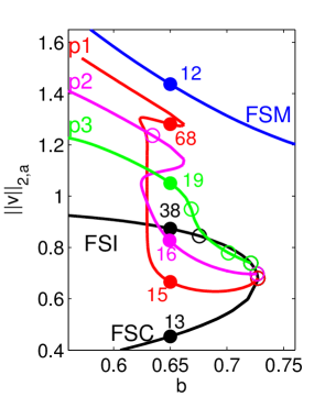
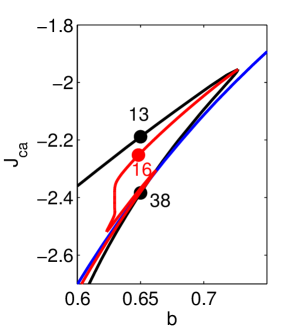
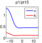
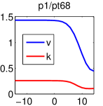
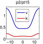
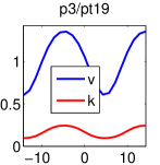
Figure 1: Example bifurcation diagrams and solution plots from running bdcmds.m. For $b<b_{\text{fold}}\approx 0.73$ there are three branches of FCSS, here called FSC (Flat State Clean, low $v$), FSI (Flat State Intermediate), and FSM (Flat State Muddy, high $v$). On FSC$\cup$FSI there are a number of bifurcations to patterned CSS branches. See [GU17] for further discussion.

2.1.2 Canonical paths

For OC problems, the computation of CSS is just the first step. The next goal is to calculate CPs from some starting state $v(0)$ to a CSS $\hat{u}_{1}$ with the SPP. For this we use the continuation algorithm isc which is essentially a wrapper for the BVP solvers mtom and bvphdw, and which for CSS as targets implements Algorithm 1. The data is again stored in a problem structure p which has a number of general options/parameters in p.oc, options specific to the behavior of the BVP solvers stored in p.tomopt, and solution data stored in p.cp. In particular, the oclib routines re–use the data and functions (FEM data, function handles) already set up for the computation of the CSS (or CPS), and no new functions need to be set up. The convenience function ocinit sets most OC parameters to standard values and, if provided with the corresponding data, the starting states and end point of the canonical path, i.e., the target CSS $\hat{u}$, or the target $\hat{u}_{0}$ on a CPS $\hat{u}$. This function is the analog of stanparam in the CSS setting. For a first call the user only has to set the parameters at the top of Table 2, the estimated truncation time and the (initial) number of mesh points. However, as usual, the user can, and sometimes has to, change some of the standard options.

(a) $P$ and $q$ on the CP from p3/pt19 to FSC	(b) diagnostics for (a)	(c) Using $T$ adaptation

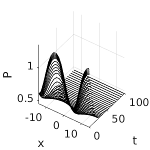
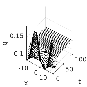
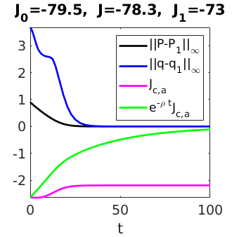
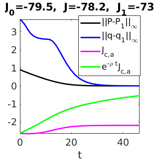
(d) Fold in $\alpha$ for continuation for CP from p1/pt68 to FSS, and “upper” canonical path at $\alpha=0.6$

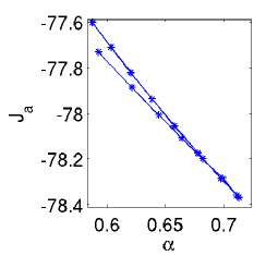
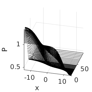
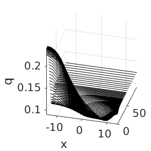
Figure 2: Example outputs from cpdemo1D.m. (a) shows $P,q$ on the CP from the patterned CSS p3/pt19 (see Fig. 1) to the ’Clean Flat State’ FSC, and (b) shows typical associated ’diagnostics’, namely the convergence behavior to $\hat{u}$ (in $\|\cdot\|_{\infty}$ norm), the current value, and the discounted current value along the CP. On top we plot the value $J_{0}$ of the ’starting’ CSS (from which we take the states), the value $J$ of the path, and the value $J_{1}$ of the target CSS. (c) shows essentially the same as (b), but starting with a rather small truncation time $T$, and then adapted during the continuation in the initial states. (d) shows a case where a CP from some states (here taken from p1/pt68) to a target CSS (here again the FSC) does not seem to exist, or at least cannot be computed by continuation in $\alpha$, due to a fold.

After setting up the data structures (via ocinit or modifications and possibly further commands) in the struct p, the computation of CPs is started by a call of p=isc(p,alvin,varargin) with default input parameters p and alvin, where alvin is a vector of continuation steps. For arclength continuation, the third input may contain the number of arclength continuation steps. For consecutive arclength calls, one can also set alvin=[] to directly start with arclength continuation. However a secant and two values for $\alpha$ have to be given via p.oc.usec and p.hist.alpha (if natural continuation was done before, these fields are filled). See Section 2.1.3 for examples and further description of isc, other OC related pde2path functions, and the parameters in p.oc and p.tomopt. Here we continue with a brief description of CP results for the SLOC problem. The canonical path related computations are done in the command files cpdemo*. We first compute paths from a patterned CSS to a flat CSS and vice versa in cpdemo1D, see Listing 5 and Figure 2, while cpdemo2D does the same in $2D$. The file skibademo, to be run after cpdemo1D, computes some Skiba paths, see §2.1.4.

struct/varname	default	description/comment
oc/		struct with controls for isc external to the BVP solvers mtom and bvphdw
nti		Initial number of mesh points. Highly problem dependent, so should be set by user. mtom has automatic mesh refinement, so rather try a small nti, while for bvphdw a somewhat larger nti should be used.
T		first guess for truncation time - if empty it is set by isc
nTp	2	for setting $T{=}{\tt nTp}{*}T_{p}$ as a guess for $T$ for CPs to a CPS, $T_{p}{=}$period of CPS
freeT	0	if 1, then truncation time is set free for CPs to CSS, and (20) is included in the BVP, with $\varepsilon$ in oc.tadev2
tv	[]	initial t-mesh if not empty, otherwise generated by isc
retsw	0	return-switch for isc: 0: only final soln, 1: solutions for all $\alpha$
msw	0	predictor in natural continuation. 0: trivial, 1: secant
rhoi	1	pde2path index of the discount rate $\rho$
tadevs	inf	target error in sup–norm, i.e., $\varepsilon_{\infty}$ in (19). Can be set initially, but we recommend a first step without $T$ adaptation (small $\alpha$), i.e., also freeT=0.
tadev2	*	target error in euclidean norm, i.e., $\varepsilon$ in (20), initialized by (21) once (19) is violated. Can be reset later to decrease the target deviation.
mtom	1	switch between mtom and bvphdw (in–house bvp solver)
sig	0.1	stepsize for arclength continuation
sigmin/sigmax	1e-2,10	minimal and maximal stepsizes for arclength continuation
fn		file–names, for instance for the initial and target states of the CP
u0		initial states; can be provided by file (see examples), or be set after ocinit
s1		classical pde2path data struct which will typically contain the data for the target $\hat{u}$ (CSS in s1.u, or CPS in s1.hopf))
tomopt/		struct with controls for the BVP solvers mtom and bvphdw
lu	0	if 0, then use \ (usually faster) instead of $LU$ decomposition in mtom
	*	Standard mtom-parameters can be given here, e.g. Itlimax, Itnlmax and Nmax for maximal number of linear and nonlinear iterations and maximal number of mesh points. See mtom documentation.
tol, maxIt	1e-8,10	tolerance (in $\|\cdot\|_{\infty}$ norm) and max nr of iterations in bvphdw.

Table 2: Data in the struct p for computing CPs. Most parameters are set to standard values via ocinit, but some are problem specific and have to be set explicitly. Others can and some usually have to be overwritten for the specific problem. Some options are not listed here or in Table 3, which are for internal or expert use only. See ocinit and isc for further comments and details.

name	description
cp.u	solution (CP) generated by isc; used as initial guess for next continuation step, if already set by previous call to isc or if set externally.
cp.t	time mesh generated by isc (or set externally)
cp.par	solution parameters, i.e., truncation time $T$ in par(1), current $\alpha$ in par(2) (for arclength)
hist.alpha	vector of the $\alpha$ values in the continuation
hist.vv	vector of the objective values of the canonical path for the $\alpha$ stored in hist.alpha
hist.u	CPs at continuation steps stored in hist.alpha
hist.t	time-meshes (normalized to $[0,1]$) of continuation steps
hist.par	parameter values ($T$ and $\alpha$) of the continuation steps

Table 3: Additional fields in p, typically set/maintained/updated by isc (p.hist only maintained/updated if oc.retsw=1).

⬇

1%% SLOC canonical paths, Cell 1: CP from p3/pt19 to f1/pt13; nat.continuation

p=[]; p=ocinit(p,’p3’,’pt19’,’f1’,’pt13’); % set standard options, also set

% p3/pt19 as start and f1/pt13 as end point of the canonical path

p.oc.rhoi=1; % index of discount rate rho, rho is at p.u(p.nu+p.nq+rhoi)

p.oc.T=100; % truncation time

6% reset some oc-params to customized values

p.oc.nti=41; % initial # of points in t-mesh

p.oc.msw=1; % use secant predictors (after first step) in isc

alvin=[0.25 0.5 0.75 1]; % desired alpha-values; these can also be split,

% e.g., first call isc with alvin=[0.25 0.5], then again with alvin=[0.75 1]

11p=isc(p,alvin); va=[15,30]; slsolplot(p,va); % continuation call and plot

%% Cell 2: start with small T, then set T free (test T adaptation)

p=[]; p=ocinit(p,’p3’,’pt19’,’f1’,’pt13’); p.oc.rhoi=1; p.oc.T=20;

p.oc.nti=41; p.oc.msw=1; p.oc.tadevs=1e-2; p.oc.verb=2;

alvin=[0.25 0.5 0.75 1]; p=isc(p,alvin);

16va=[15,30]; slsolplot(p,va); tadev(p); % some plots

%% Cell2b: decrease ||u(1)-\uhat|| (increasing T from 43 to about 50)

p2=p; p2.oc.tadevs=1e-4; p2=isc(p2,1); slsolplot(p2,va); tadev(p2);

ocdemos/sloc/cpdemo1D.m

Listing 5: Cells 1 and 2 from sloc/cpdemo1D.m (to be run after bdcmds1D.m). We compute a CP from the states of p3/pt19 to the CSS f1/pt13 by ‘‘natural continuation’’ in the initial states. In the remainder of cpdemo1D we illustrate arclength continuation (also in preparation of skibademo), and the extraction of data from the continuation history.

2.1.3 Main oclib functions

The functions ocinit and isc are the main user interface functions for CP numerics. Essentially, after having set up p as in §2.1.1 for the CSS, including p.fuha.jcf, the user does not need to set up any additional functions to calculate canonical paths and their values. We give the signatures and some general remarks on the arguments and behavior of ocinit and isc, with the Cells referring to Listing 5.

• Convenience function (similar to p=stanparam(p)) to generate a standard problem structure p where most parameters are set to standard values. These are parameters for mtom (see tom/tomset.m), and parameters for isc, see Table 2 for an overview. If varargin={sd0,sp0,sd1,sp1}, then ocinit also sets the states of the solution stored in sd0/sp0 as the starting states and the solution stored in sd1/sp1 as the aimed CSS/CPS. Typically some of the options should be overwritten in the further setup.

• p is the problem structure containing the options/parameters described above in p.oc and p.tomopt, see Tables 2 and 3, and the solution in p.cp. alvin is the vector of desired $\alpha$ values for the continuation, for instance alvin=[0.25 0.5]. If varargin=nsteps is given as a third input, arclength continuation is started after the last value of alvin with nsteps steps, or until $\alpha=1$ is reached. If previous calls of isc are present, then we can directly start arclength continuation by calling isc with empty alvin. After the first call of isc some additional fields are set in p.oc, containing, e.g., the current secant, the last starting point in the continuation, and, if desired via p.oc.retsw=1, the solutions at different continuation steps, see Table 3.

Remark 2.1.

Concerning the original TOM options we typically run isc with weak error bounds and what appears to be the fastest monitor and order options, i.e., tomopt.Monitor=3; tomopt.order=2. Once continuation is successful (or also if it fails at some $\alpha$), we can always postprocess by calling mtom again with a higher order, stronger error requirements, and different monitor options. See the original TOM documentation. The most convenient way to do so is to call isc with alvin=1 again after resetting TOM-related options. $\rfloor$

There are a number of additional functions for internal use, and some convenience functions, which we briefly review as follows:

• For CPs to CSSs only: compute $\Psi$, the eigenvalues mu, the defect d, and a suggestion for $T$. This becomes expensive with large $2nN$ (number of spatial DoF).

• For CPs to CPSs only: computes (by periodic Schur decomposition) the projection on the center-unstable eigenspace in Fu2 and the Floquet-multiplicators in d. Expensive, but has to be done only once for each CPS.

• Modification of TOM, which allows for $M$ in (15a). Extra arguments $M$ and lu,vsw in opt. If opt.lu=0, then $\backslash$ is used for solving linear systems instead of an LU–decomposition, which becomes too slow when $2nN\times m$ becomes too large. See the TOM documentation for all other arguments included in opt, and note that the modifications in mtom can be identified by searching “HU” in mtom.m. Of course mtom (as any other function) can also be called directly, which for instance can be useful to postprocess the output of some continuation by changing parameters by hand.

• A simple Newton solver for CPs, which was mainly used for testing but is sometimes more robust than the sophisticated methods (error estimation and mesh refinement) of mtom.

• The rhs and its Jacobian to be called within mtom resp. bvphdw (see the respective wrapper files). These are wrappers which calculate $f$ and $J$ by calling the resp. functions in the pde2path–struct p.opt.s1, which were already set up and used to calculate the CSS/CPS. Similar remarks apply to mrhse and fjace for the arclength continuation.

• The boundary conditions (in time) for (15) resp. (36) and the associated Jacobians again with wrappers to be used for mtom and bvphdw at once. The *e (as in extended) versions are for arclength continuation again.

• Computes the value

  $${\tt jval}=J(u)=\int_{0}^{T}{\rm e}^{-\rho t}J_{ca}(v(t,\cdot),q(t,\cdot))\,{\rm d}t$$ (47)

  of the solution $u$ in cp (with $J_{c}$ taken from s1.fuha.jcf), and also returns $J_{ca}$ and ${\rm e}^{-\rho t}J_{ca}$ along the CP for easy plotting, cf. Fig. 2(b).

• Deviations (in sup norm and euclidean norm) of endpoint of CP from target, see (19) and (20).

Remark 2.2.

There are also some plotting function in oclib, which however should be seen as templates for plotting of canonical paths, including diagnostic plots to check the convergence behavior of the canonical path as $t\rightarrow T$, cf. (d),(f) in Fig. 2. The function slsolplot(p,view) in the sloc demo directory can serve as a template how to set up such plots. $\rfloor$

2.1.4 Skiba points

In ODE OC applications, if there are several locally stable CSS, then often an important issue is to identify their domains of attractions. These are separated by so called threshold or Skiba–points (if $N=1$) or Skiba–manifolds (if $N>1$), see [Ski78] and [GCF⁺08, Chapter 5]. Roughly speaking, these are initial states from which there are several optimal paths with the same value but leading to different CSS. Here we give an example for the SLOC model how to compute a patterned Skiba point between FSC and FSM.

In Cell 3 of cpdemo1D.m we attempt to find a path from $v_{\text{PS}}$ given by p1/pt68 to $(v,q)_{\text{FSC}}$ given by FSC/pt13; this fails due to the fold in $\alpha$. However, for given $\alpha$ we can also try to find a path from the initial state $v_{\alpha}(0):=\alpha v_{\text{PS}}+(1-\alpha)v_{\text{FSC}}$ to the FSM, and compare to the path to the FSC. For this, we can use the problem structure p computed in Cell 3. The initial states for the k’th $\alpha$ value of p.hist.alpha are, due to p.opt.retsw=1, stored in p.hist.u{k}(:,1) i.e. as the starting point of the canonical path associated to the given $\alpha$ value.

In skibademo.m (Listing 10, which is a rather elaborate application of the OC facilities of pde2path, and can be skipped on first reading) we find paths from these initial states from cpdemo1D.m to the other flat steady state with the SPP, namely FSM, and compare the values with the values of the paths to FSC, stored in p.hist.vv. See Fig. 3 for illustration.

(a) A Skiba point at $\alpha=0.454$	(b) Paths to FSC (blue) and FSM (red)

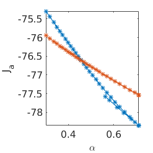
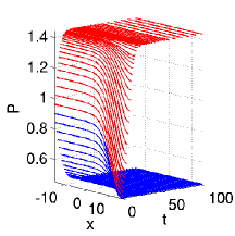
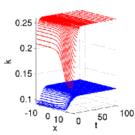
Figure 3: Example outputs from skibademo.m. For the ($\alpha$–dependent) initial states from the path from p1/pt68 to the FSC from cpdemo1D (blue curve in (a)), we compute the CPs to the FSM, yielding the red curve in (a). Near $\alpha=0.43$ the two CPs have the same values, which makes these initial states a so–called Skiba candidate. (b) shows the two associated CPs of equal value.

⬇

1% Skiba example, continues cpdemo1D.m

% Either run Cells 3 and 4 from cpdemo1D or, if storing was enabled there,

% load the continuation from p1/pt68 to f1/pt13 via load(’skibap.mat’)

vv=[]; % vector for objective values of paths to f2/pt12, and same for al, sols

alv=[]; sol={}; doplot=1; alvin=[0.1 0.25 0.5 0.75 1]; v=[30 30];

6for k=1:30 % loop all computed al values from old path

p2=[]; p2=ocinit(p2,’p1’,’pt68’,’f2’,’pt12’);

p2.oc.s0.u(1:42)=p.hist.u{k}(:,1); % reset starting states

p2.oc.rhoi=1; p2.oc.nti=10; p2.oc.T=100; % options

p2=isc(p2,alvin); % continuation call

11 alv=[alv p.hist.alpha(k)]; vv=[vv p2.hist.vv(end)]; % store al, Jc

Jd=p.hist.vv(k)-vv(end);

sol{k}=p2.cp; % store solutions

if abs(Jd)<0.05; doplot=asknu(’plot path?’,doplot); % Skiba point(s) found

if doplot==1 % plot the paths to FSC and FSM

16 sol1.u=p.hist.u{k}; sol1.t=p.hist.tt{k}; sol1.par=p.hist.par{k};

psol3Dm(p.oc.s1,sol{k},sol1,1,1,[]); view(v); zlabel(’P’);

psol3Dm(p.oc.s1,sol{k},sol1,2,0,[]); view(v); zlabel(’k’); pause

end

end

21end

ocdemos/sloc/skibademo.m

Listing 6: sloc/skibademo.m. Using the data stored in p.hist.* in Cell 3 of cpdemo1D.m (for $b=0.65$), we compute canonical paths from the initial states to the FSM at $b=0.65$, and compare the objective values with those stored in p.hist.vv (for the path to the FSC). If both are sufficiently close, then we have a good approximation of a Skiba point. Thus, in line 6 we start a loop over the $\alpha$ values generated in cpdemo1D.m; in line 8 we put the associated initial states into p2.opt.s0, i.e. overwrite the loaded point, and then (line 10) find the canonical path to the FSM. In line 14 we check if we found a Skiba point approximation, in which case we plot both paths. Also the second cell then deals with plotting.

Remark 2.3.

The directory slocdemo also contains the script files bdcmds2D.m and cpdemo2D.m, used to compute CSS and canonical paths for (45) over the 2D domain $\Omega=(-L,L)\times(-\frac{L}{2},\frac{L}{2})$ (based on exactly the same init file slinit.m), and some modified plotting functions plotsolf.m and plotsolfu.m, see, e.g., [GU17, Fig. 4,5] for some 2D results. $\rfloor$

2.2 Optimal harvesting patterns in a vegetation model

Our second example, from [Uec16], concerns the optimal control of a reaction diffusion system used to model harvesting (or grazing by herbivores) in a system for biomass (vegetation) $v$ and soil water $w$, following [BX10]. Denoting the harvesting (grazing) effort as the control by $E$, we consider

$$V(v_{0},w_{0}) =\max_{E(\cdot,\cdot)}J(v_{0},w_{0},E),$$ (48a)

$${\partial}_{t}v =d_{1}\Delta v+[gwp^{\eta}-d(1+\delta v)]v-H,$$ (48b)

$${\partial}_{t}w =d_{2}\Delta w+R(\beta+\xi v)-(r_{u}v+r_{w})w,$$ (48c)

with harvest $$H=v^{\alpha}E^{1-\alpha} J_{c}=J_{c}(v,E)=pH-cE p c v E 0<\alpha<1$$, and current value objective function , which thus depends on the price , the costs for harvesting/grazing, and , in a classical Cobb–Douglas form with elasticity parameter . Furthermore, we have the boundary conditions and initial conditions

$${\partial}_{\nu}v={\partial}_{\nu}w=0\text{ on }{\partial}\Omega,\quad(v,w)|_{t=0}=(v_{0},w_{0}).$$ (48d)

Again we want to maximize the discounted profit

$$J=\int_{0}^{\infty}{\rm e}^{-\rho t}J_{ca}(v,E)\,{\rm d}t.$$ (49)

For the modeling, and the meaning and values of the parameters $(g,\eta,d,\delta,\beta,\xi,r_{u},r_{w},d_{1,2})$ we refer to [BX10, Uec16], and here only remark that the model aims at a realistic description of certain semi–arid systems, that, e.g., the discount rate $\rho=0.03$ is in the pertinent economic regime, and that, like in most studies of semi–arid systems, we take the rainfall $R$ as the main bifurcation parameter.

Denoting the co-states by $(\lambda,\mu)$ we obtain the canonical system

$${\partial}_{t}v =d_{1}\Delta v+[gwp^{\eta}-d(1+\delta v)]v-H,$$ (50a)

$${\partial}_{t}w =d_{2}\Delta w+R(\beta+\xi v)-(r_{u}v+r_{w})w,$$ (50b)

$${\partial}_{t}\lambda =\rho\lambda-p\alpha v^{\alpha-1}E^{1-\alpha}-\lambda\bigl{[}g(\eta+1)wv^{\eta}-2d\delta v-d-\alpha v^{\alpha-1}E^{1-\alpha}]-\mu(R\xi-r_{u})w-d_{1}\Delta\lambda,$$ (50c)

$${\partial}_{t}\mu =\rho\mu-\lambda gv^{\eta+1}+\mu(r_{u}v+r_{w})-d_{2}\Delta\mu,$$ (50d)

where $$E\left(\frac{c}{(p-\lambda)(1-\alpha)}\right)^{-1/\alpha}v$$.

The system (50) has a similar structure as (45), with the immediate difference that (50) has four components and many parameters, and thus looks somewhat complicated. However, it is still convenient to implement in pde2path, and leads to many patterned optimal steady states, see [Uec16] for further discussion. Thus, besides documenting the implementation of (50) underlying the results in [Uec16], our aim here is to illustrate that also rather complicated systems can be implemented and studied in the pde2path OC setting in a simple way. Writing (50) as ${\partial}_{t}u=-G(u)$, $u=(v,w,\lambda,\mu)$, we basically need to set up the domain, $G$ and the BCs, and the objective function. Table 4 lists and comments on the scripts and functions in ocdemos/vegoc. The implementation of (50) follows the general pde2path settings with the OC related modifications already explained in §2.1, and thus we only give a few remarks in the Listing captions.

Table 4: Scripts (1D) and functions in ocdemos/vegoc; oosetfemops and veginit (which also contains the parameter values) as usual; the bottom part contains ’helper’ functions for plotting.

script/function	purpose,remarks
bdcmds, cpcmds	scripts to compute CSS and canonical paths
efu, vegjcf	functions to compute [E,H] from u, and the current value $J_{c}$ (by calling efu)
vegsolplot, vegdiagn	functions to plot CPs, and compute and plot diagnostics for CPs
vegcm.asc, watcm.asc	colormaps for CP plots (and state plots in 2D)

⬇

1function [e,h,J]=efu(p,varargin) % extract [e,h,J] from p.u or u

if nargin>1 u=varargin{1}; else u=p.u; end

par=p.u(p.nu+1:end); cp=par(11); pp=par(12); al=par(13);

v=u(1:p.np); l1=u(2*p.np+1:3*p.np);

gas=((pp-l1)*(1-al)./cp).^(1/al); e=gas.*v; h=v.^al.*e.^(1-al);

6J=pp*v.^al.*e.^(1-al)-cp*e;

Listing 7: vegoc/skibademo.m. Using the data stored in p.hist.* in Cell 3 of cpdemo1D.m (for $b=0.65$), we compute canonical paths from the initial states to the FSM at $b=0.65$, and compare the objective values with those stored in p.hist.vv (for the path to the FSC). If both are sufficiently close, then we have a good approximation of a Skiba point. Thus, in line 6 we start a loop over the $\alpha$ values generated in cpdemo1D.m; in line 8 we put the associated initial states into p2.opt.s0, i.e. overwrite the loaded point, and then (line 10) find the canonical path to the FSM. In line 14 we check if we found a Skiba point approximation, in which case we plot both paths. Also the second cell then deals with plotting.

⬇

1function r=vegsG(p,u) % rhs for vegOC problem

par=u(p.nu+1:end); rho=par(1); g=par(2); eta=par(3); % extract param

d=par(4); del=par(5); beta=par(6); xi=par(7); rp=par(8);

up=par(9); rw=par(10); pp=par(12); al=par(13);

v=u(1:p.np); w=u(p.np+1:2*p.np); % extract soln-components, states

6l1=u(2*p.np+1:3*p.np); l2=u(3*p.np+1:4*p.np); % co-states lam1, lam2

[e,h]=efu(p,u); % get effort E and harvest h

f1=(g*w.*v.^eta-d*(1+del*v)).*v-h;

f2=rp*(beta+xi*v)-(up*v+rw).*w;

f3=rho*l1-pp*al*h./v-l1.*(g*(eta+1)*w.*v.^eta-2*d*del*v-d-al*h./v)...

11 -l2.*(rp*xi-up*w);

f4=rho*l2-l1.*(g*v.^(eta+1))-l2.*(-up*v-rw);

f=[f1;f2;f3;f4]; % the ’nonlinearity’ (everything but diffusion)

r=p.mat.K*u(1:p.nu)-p.mat.M*f; % the residual

Listing 8: vegoc/efu.m and vegsG. efu computes the harvesting effort (control) $E$, the harvest $h$ and the current value $J$, hence also called in vegoc/vegjcf.m. In vegsG we first extract the parameters and the solution components, and compute $H$ (from efu). Then we implement the ’nonlinearity’ in a straightforward way, and compute the residual $G$ using the preassembled stiffness and mass matrix (see oosetfemops.

Figure 4 shows a basic bifurcation diagram of CSS in 1D with $\Omega=(-L,L)$, $L=5$, from the script file bdcmds.m, which follows the same principles as the one for the SLOC demo. Again we start with a spatially flat (i.e., homogeneous) canonical steady FSS (black), on which we find a number of Turing-like bifurcations. The blue branch in (a) represents the primary bifurcation of PCSS (patterned canonical steady states), which for certain $R$ have the SPP, and, moreover, turn out to be POSS (patterned optimal steady states). See [Uec16] for more details, including a comparison with the uncontrolled case of so called “private optimization”, and 2D results for $\Omega=(-L,L)\times(-\sqrt{3}L/2,\sqrt{3}L/2)$ yielding various POSS, including hexagonal patterns.

(a)                                                                          (b)                                           (c)
 

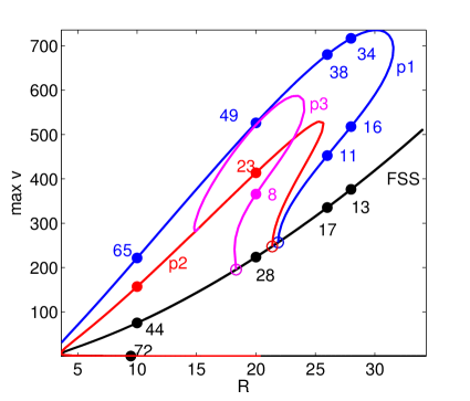
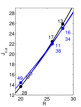
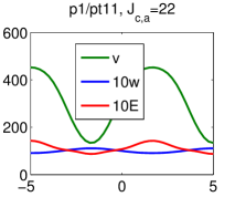
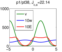
Figure 4: Example outputs of bdcmds.m. (a),(b) bifurcation diagrams of CSS in 1D; (c) example solutions.

The script files cpcmds.m for CPs, and skibacmds.m for a Skiba point between the flat optimal steady state FSS/pt13 and the POSS p1/pt34, again follow the same principles as in the the SLOC demo. See Figure 5 for an example output. We use customized colormaps for vegetation (green) and water (blue), which are provided as vegcm.asc, watcm.asc and whitecm.asc, respectively.

(a)	(b)

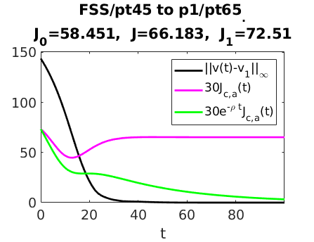
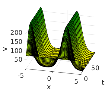
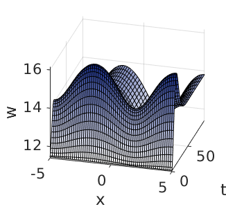
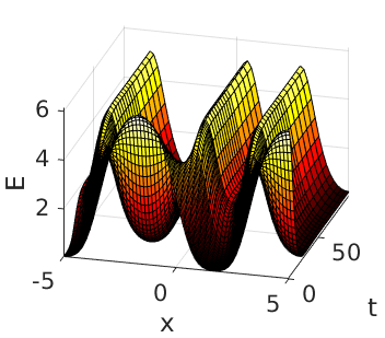
Figure 5: Example output of vegoc/cpcmds.m, namely the canonical path from the (states of the) lower FCSS(FSS/pt45) (cf. Fig. 4) to the PCSS (p1/pt65) at $R=10$. (a) shows the convergence behavior, the current value profit, and obtained objective value. (b) show $(v,w)$ and the harvesting strategy $E$. In particular, the values $J_{0}$ of the starting CSS, $J$ of the CP, and $J_{1}$ of the target CSS show that here controlling the system from the flat CSS to the PCSS yields a significantly higher value. See [Uec16] for further comments and more details.

2.3 Optimal boundary catch as an example of boundary control

Our third example, taken from [GUU19], considers the optimization of the discounted fishing profit $J=\int_{0}^{\infty}{\rm e}^{-\rho t}J_{c}(v(0,t),q(t))\,{\rm d}t$, $\displaystyle J_{c}(v,q)=\sum_{j=1}^{2}p_{j}h_{j}(v_{j},q_{j})-c_{j}q_{j}$. Here $v=(v_{1},v_{2})$ are the populations of two fish species ($v_{1}=$prey, $v_{2}=$predator) in a (1D) lake or ocean $\Omega=(0,l_{x})$, $q=(q_{1},q_{2})$ are the fishing (harvesting) efforts (controls) of $v_{1}$ and $v_{2}$, respectively, at the shore, and $p_{1,2}$ and $c_{1,2}$ are the prices for the fishes and the costs for fishing, respectively, and we again choose a Cobb–Douglas form for the harvests $h_{j}(v_{j},q_{j})=v_{j}^{\alpha_{j}}q_{j}^{1-\alpha_{j}}$, with parameters $\alpha_{j}\in(0,1)$. We assume that the fish populations evolve according to a standard Lotka-Volterra model, namely

$$\begin{split}{\partial}_{t}v_{1}&=d_{1}\Delta v_{1}+(1-\beta v_{1}-v_{2})v_{1},\\ {\partial}_{t}v_{2}&=d_{2}\Delta v_{2}+(v_{1}-1)v_{2},\end{split}\quad\text{or ${\partial}_{t}v=-G_{1}(v)=D\Delta v+f(v)$,}$$ (51)

in $\Omega$, with $D=\begin{pmatrix}d_{1}&0\\ 0&d_{2}\end{pmatrix}$ and growth function $f(v)=\begin{pmatrix}(1-\beta v_{1}-v_{2})v_{1}\\ {(v_{1}-1)v_{2}}\end{pmatrix}$, with parameter $\beta>0$. The controls $q_{1,2}$ (fishing efforts for species $v_{1,2}$, respectively) occur in the BCs for (51), i.e., we assume the Robin BCs

$$d_{j}{\partial}_{n}v_{j}=-g_{j}:=-\gamma_{j}h_{j},\quad j=1,2,\text{ at $x=0$},$$ (52)

and zero flux BCs ${\partial}_{n}v_{j}=0$ at $x=l_{x}$. Thus, in contrast to the sloc and vegoc examples we no longer have a spatially distributed control, but a (two component) boundary control.

Introducing the co-states $\lambda_{1,2}:\Omega\rightarrow{\mathbb{R}}$, Pontryagin’s maximum principle yields the evolution and the BCs of the co-states (combining with (51), to have it all together)

$$\left.\begin{array}[]{l}{\partial}_{t}v=D\Delta v+f(v),\\ {\partial}_{t}\lambda=\rho\lambda-D\Delta\lambda-({\partial}_{v}f(v))^{T}\lambda\end{array}\right\}\quad\text{ in $\Omega=(0,l_{x})$},$$ (53c)

$$\left.\begin{array}[]{l}D{\partial}_{n}v+g=0,\\ D{\partial}_{n}\lambda+{\partial}_{v}g(v)\lambda-{\partial}_{v}J_{c}=0,\end{array}\right\}\quad\text{ on the left boundary $x=0$},$$ (53f)

$$\left.\begin{array}[]{l}D{\partial}_{n}v=0,\\ D{\partial}_{n}\lambda=0,\end{array}\right\}\quad\text{ on the right boundary $x=l_{x}$},$$ (53i)

and

$$q_{j}=\left(\frac{(1-\alpha_{j})^{2}(p_{j}-\gamma_{j}\lambda_{j})}{c_{j}}\right)^{1/\alpha_{j}}v_{j},\text{ evaluated at the left boundary $x=0$},\quad j=1,2.$$ (53j)

See [GUU19] for details on the derivation of (53).

Thus, we again have a 4 component reaction diffusion system (53a-c) for the states $v$ and the costates $\lambda$, but now the controls live on the boundary at $x=0$, leading to nonlinear flux boundary conditions. Also, from the modeling point of view, the pertinent questions for (53) are slightly different than for (50), since for (53) we are not so much interested in bifurcations and pattern formation (which do not occur for the parameters chosen below), but rather in the dependence of the (unique) CSS on the parameters, and mostly in the canonical paths leading to these CSS.

In any case, we now focus on how to put the nonlinear BCs into pde2path. Table LABEL:lvoctab lists the scripts and functions in ocdemos/lvoc, and some further comments are given in the listing captions below.

Table 5: Scripts and functions in ocdemos/lvoc; the first four follow closely the same pde2path principles as the respective functions in sloc and vegoc. lvsG is a rather non–generic implementation of the rhs of (53), and in particular strongly uses the 1D nature of the problem. The others are naturally also problem specific, and in particular the last three overload some pde2path standard functions.

script/function	purpose,remarks
bdcmds,cpcmds	scripts to compute CSS and CPs
lvinit,oosetfemops	init routine, and setting of FEM matrices
lvsG	the rhs for (53a), also explicitly implementing the BC (53b), while (53c) are naturally fulfilled with K the Neumann Laplacian.
lvbra	branch-output, here substantially modified from stanocbra, i.e., writing specific data like profits/harvest/controls per fish-species on the branch
hfu	returns harvest $h\in{\mathbb{R}}^{2}$, and derivatives (needed for lvsG) ${\partial}_{v}h\in{\mathbb{R}}^{2\times 2}$, ${\partial}_{k}h\in{\mathbb{R}}^{2\times 2}$; straightforward implementation.
lvjcf	returns $J_{c}$, as required in the standard pde2path setup for OC problems, but also the individual profits $J_{1,2}$ per fish-species.
jca	$J_{c}$ average, overloaded here since $J_{c}$ is on boundary, hence the default averaging by $1/|\Omega|$ makes no sense
lvdiagn	diagnostics functions for canonical paths
stanpdeo1D${<}$pde	classdef, overloads the pde2path classdef stanpdeo1D in order to have $\Omega=(0,l_{x})$ instead of $\Omega=(-l_{x},l_{x})$ (standard).
plotsol, psol3D	some more overloads of pde2path standard functions for plotting.

Figure 6 gives some example plots from running bdcmds.m. This script is rather lengthy, with the main point here to illustrate how to plot various data of interest by first putting it on the branch (here via lvbra.m) and then choosing the pertinent component for plotting. The script cpcmds.m for computing canonical paths follows the same outline as those for the sloc and vegoc examples. Figure 7 shows a canonical path to the CSS at $c=(0.1,0.1)$, starting from the homogeneous fixed point $V^{*}=(1,1-\beta)$ of (51). As already said, we refer to [GUU19] for discussion of the results.

(a) $J,v$ and $q$ at $x=0$; continuation in $c_{1}$	(b) CSS at $c=(0.1,0.1)$

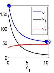
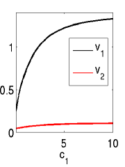
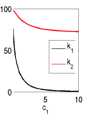
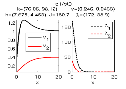
Figure 6: (a) continuation diagrams in $c_{1}$ (costs for prey fishing); $J_{j}=p_{j}h_{j}-c_{j}q_{j}$, $J=J_{1}+J_{2}$. (b) An example CSS plots.

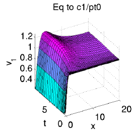
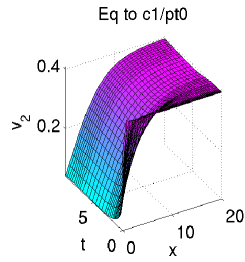
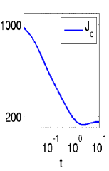
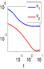
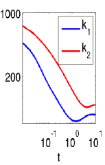
Figure 7: A CP starting from the spatially homogeneous steady state $V^{*}$ of (51) to the CSS at $(c_{1},c_{2})=(0.1,0.1)$. Note the logarithmic scales in the time-series of the values at the left boundary.

⬇

1function r=lvsG(p,u) % rhs for lvoc.

n=p.np; par=u(p.nu+1:end); beta=par(1); d1=par(4); d2=par(5);

ga1=par(6); ga2=par(7); rho=par(8); p1=par(11); p2=par(12); % extract pars

v1=u(1:n); v2=u(n+1:2*n); l1=u(2*n+1:3*n); l2=u(3*n+1:4*n); % extract fields

f1=v1.*(1-beta*v1-v2); f2=(v1-1).*v2; % bulk nonlin.

6a11=1-2*beta*v1-v2; a12=-v1; a21=v2; a22=v1-1;

f3=rho*l1-a11.*l1-a21.*l2; f4=rho*l2-a12.*l1-a22.*l2;

f=[f1; f2; f3; f4]; F=p.mat.M*f; % bulk finished, no go to BCs

l11=l1(1); l21=l2(1); [h,hv,hk]=hfu(p,u); % bd vals of lambda, and harvest

g1=-ga1*h(1); g2=-ga2*h(2); % BC for states

11g3=-(p1-ga1*l11)*hv(1); g4=-(p2-ga2*l21)*hv(4); % BC for co-states

F(1)=F(1)+g1; F(n+1)=F(n+1)+g2; % add BC directly into F, states

F(2*n+1)=F(2*n+1)+g3; F(3*n+1)=F(3*n+1)+g4; % BC for co-states

zM=0*speye(n); K=p.mat.K; % finally assemble the system K

16K=[[d1*K zM zM zM]; [zM d2*K zM zM]; [zM zM -d1*K zM]; [zM zM zM -d2*K]];

r=K*[v1;v2;l1;l2]-F; % and compute the residual as usual

Listing 9: lvoc/lvsG.m. As usual we first extract the relevant parameters and fields from $u$, and compute the ’bulk’ nonlinearity $f$ (i.e., the nonlinearity in $\Omega$). Then, to compute the BCs we first extract values of the co-states on the boundary, and the associated harvests and their derivatives. These are needed to compute the BCs $g_{j}$, $j=1,\ldots,4$ (lines 13,14), which can then directly be added to the rhs on the boundary (lines 16,17). Here we strongly use the 1D setup, i.e., that the left boundary value of component $j$ is at u((j-1)*np+1), where np is the number of spatial discretization points. In line 19 we then assemble the system $K$. Compared to the setup in vegoc/vegsG this has the advantage that the diffusion constants $d_{1,2}$ can be used like any other parameter at this point. The actual computation of r in line 20 then works as usual.

3 Examples and implementation details for CPs to CPSs

The basic idea for the computation of CPSs and of CPs to CPSs is similar to that for the computation of CSSs and CPs to CSSs. We first search for CPSs, usually via Hopf bifurcations from CSSs, and then aim to compute CPs $u$ to such CPSs with the SPP, again using the main pde2path OC user interface isc, which now implements Algorithm 2. To illustrate the setup we first discuss an ODE toy model. Subsequently we come to a PDE model for pollution mitigation.

3.1 An ODE toy problem

We start with the ODE toy model

$$\dot{x_{1}}=\rho\left(-x_{1}-\frac{\theta x_{2}}{\rho}+x_{1}y_{1}r^{2}\right),\quad\dot{x_{2}}=\rho\left(-x_{2}+\frac{\theta x_{1}}{\rho}+x_{2}y_{1}r^{2}\right),$$ (54a)

$$\dot{y_{1}}=\omega y_{2},\quad\dot{y_{2}}=\omega\sin(2\pi y_{1}),$$ (54b)

with parameters $\rho,\omega,\theta>0$ and $r=\sqrt{x_{1}^{2}+x_{2}^{2}}$. Although (54) is not derived as a canonical system for an OC problem, we interpret $x=(x_{1},x_{2})$ as states and $y=(y_{1},y_{2})$ as costates and call a time periodic solution of (54) a CPS.

3.1.1 Preliminary analytical remarks

Concerning our points of interest, the model (54) can almost completely be treated analytically and thus can be used to test our numerical methods. For fixed $y_{1}>0$, the nonlinear system (54a) has the unstable periodic orbit $r=1/\sqrt{y_{1}}$ of period $2\pi/\theta$, and (54a) is coupled to (or driven by) by the nonlinear pendulum (54b). In detail, by polar coordinates in $\left(x_{1},x_{2}\right)$, (54) transforms to

$$\dot{r}=\rho(-r+y_{1}r^{3}),\quad\dot{\varphi}=\theta,$$ (55a)

$$\dot{y_{1}}=\omega y_{2},\quad\dot{y_{2}}=\omega\sin(2\pi y_{1}),$$ (55b)

with $\varphi=\arg(x_{1},x_{2})$ and $r=\sqrt{x_{1}^{2}+x_{2}^{2}}$, with the phase portraits of the $r$ ODE (for fixed $y_{1}$) and the $y$ system sketched in Fig.8(a,b). Thus, to find a CPS we look for CSS of the reduced system

$$\dot{r}=\rho(-r+y_{1}r^{3}),$$

$$\dot{y_{1}}=\omega y_{2},\quad\dot{y_{2}}=\omega\sin(2\pi y_{1}).$$

The costates are independent of the states and the $\dot{y}$ system has the first integral $E(y_{1},y_{2})=\frac{1}{2}y_{2}^{2}+\frac{\omega^{2}}{2\pi}\cos(2\pi y_{1})$, i.e. solutions of the system lie on contour lines of $E$, see Fig.8(a). We choose $y_{1}\in{\mathbb{N}}$, $y_{2}=0$ and $r=\frac{1}{\sqrt{y_{1}}}$, which yields a $2\pi$ periodic solution in the full system. We fix $(\rho,\theta)=(1,1)$ and one of these CPS, namely

$$\hat{u}(t)=\left(r(t),\varphi(t),y_{1}(t),y_{2}(t)\right)=\left(1,t,1,0\right)$$ (56)

as our CPS of interest and aim to compute canonical paths to $\hat{u}$.

(a)	(b)	(c)

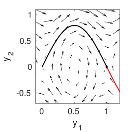
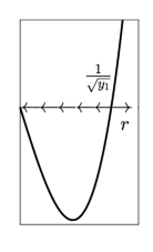
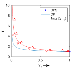
Figure 8: (a) Phase portraits of the “control system” for $y$ with the heteroclinic orbits from $(0,0)$ to $(1,0)$ and from $(2,0)$ to $(1,0)$ (red orbit, partial plot). (b) The behavior of the $r$ system. (c) Sketch of the expected CPs in the $y_{1}$–$r$–plane (using actual numerics for parameter values $(\omega,\rho,\theta)=(1,1,1)$ and initial state $(x_{1},x_{2})(0)=(4,0)$. The red line shows the nullcline $r=1/\sqrt{y_{1}}$, above (below) which he have $\dot{r}>0$ ($\dot{r}<0$). As $r(0)=\|x(0)\|>1$ we must start below the red–line by choice of $0<y_{1}(0)<1$. Together, the costates $(y_{1},y_{2})(0)$ must be on the heteroclinic to $y=(1,0)$ such that $y_{1}(t)$ increases in $t$ in such a way that $r(t)\to 1$ as $t\to\infty$.

Now given an initial state $(x_{1},x_{2})(0)$ with, e.g., $\|x\|>1$ and aiming at a CP to $\hat{u}$, i.e., the CPS associated with $(r,y_{1})=(1,1)$, we have the situation sketched in Fig.8(c). The only possible co-state choice to end in the CPS lies on the heteroclinic connection from $(y_{1},y_{2})=(0,0)$ to $(1,0)$. Thus, $y_{1}$ which is the only costate which influences the states, can take values in $\left[0,2\right]$. The state dynamics are sketched by the red triangles for $\dot{r}$ with $\dot{r}<0$ ($\dot{r}>0$) for $r<1/\sqrt{y_{1}}$ ($r>\sqrt{y_{1}}$). Since $r(0)>1$ we need to choose $y_{1}(0)>0$ sufficiently small such that $r(0)<1/\sqrt{y_{1}(0)}$ to have $\dot{r}<0$, and at the same time we need $(y_{1}(0),y_{2}(0))$ on the black $y$–heteroclinic to $(1,0)$. The argument for $\frac{1}{\sqrt{2}}<\|x_{0}\|<1$ works similarly.

We can also explicitly compute the Floquet multipliers of $\hat{u}$ and the associated projections. In polar coordinates, the variational equation (37) is autonomous, namely

$$\dot{v}=J_{f}(\hat{u})v,\quad J_{f}(\hat{u})=\begin{pmatrix}2\rho&0&0&0\\ 0&0&0&0\\ 0&0&0&\omega\\ 0&0&2\pi\omega&0\end{pmatrix},$$ (57)

with eigenvalues $\mu=(0,-\sqrt{2\pi}\omega,2\rho,\sqrt{2\pi}\omega)$. Since (57) is autonomous we obtain the multipliers by exponentiation of $\mu$, namely

$$\gamma=(\gamma_{1},\gamma_{2},\gamma_{3},\gamma_{4})=(1,\exp(-\sqrt{2\pi}2\pi\omega/\theta),\exp(4\pi\rho/\theta),\exp(-\sqrt{2\pi}2\pi\omega/\theta)).$$ (58)

Clearly, additional to the trivial multiplier we have one stable multiplier $\gamma_{2}$ and two unstable multipliers $\gamma_{3,4}$. Similarly, we can also compute the projection $P$ onto the center unstable eigenspace in Cartesian coordinates (which depends on the target point $\hat{u}_{0}$) analytically. Moreover,

$$\gamma_{2}\nearrow 1 \omega\to 0 \theta\to\infty$$ as or , (59)

and conversely $\gamma_{2}\searrow 0$ as $\omega\to\infty$ or $\theta\to 0$, and this (and the analytical projection, implemented in a testing function anaproj) can be used to tune and test the convergence behavior of the CPs in the numerics.

3.1.2 pde2path implementation and results

Table 6 lists the main files for the implementation of (54). Even though we do not need the bifurcation methods of pde2path, we implement the ODE (54) as a pde2path problem via the convenience function toyinit, because the OC routines reuse these basic pde2path data structures. To show the setup, in cmds_basic (Listing 11), we compute some CPs with easy parameter settings, namely $(\rho,\omega,\theta)=(1,1,1)$, which yields $\gamma_{2}\approx 10^{-7}$ for the “leading” Floquet multiplier, and hence fast convergence to the CPS. See Fig. 9 for some basic results, which were also used to generate the blue curve in Fig. 8(c). For convenience we outsourced the main setup in ocinit_sp, see Listing 12, which also recalls the meaning of the most important parameters. Additionally, there are some helper functions for plotting.

cmds_basic	computes canonical paths with easy parameter setting.
cmds_advanced	canonical paths with advanced parameter setting, i.e. Floquet-multipliers near $1$.
toyinit	init routine; set the limit cycle as a pde2path struct with standard parameters.
ocinit_sp	local extension of ocinit, resetting a number of parameters
sG, sGjac	rhs side of (54) resp. the Jacobian
anaproj	computes the monodromy matrix analytically

Table 6: Main scripts and functions in ocdemos/toy.

⬇

1%% Basic canonical paths of ODE toy system, Cell1, initialization

p=[]; poc=[]; nt1=40; nt2=4*nt1; % # of time-slices for CPS and CP (initial)

om=1; rho=1; th=1; par=[om;rho;th]; % parameters

p=toyinit(p,2,nt1,par); % construction of explicit CPS; now initialize CP data,

% with mtom (0/1), end-error (derr) and length wT in multiples of CP-length

6mtom=1; tadevs=1e-4; poc=ocinit_sp(poc,p,[4;0;0;0],nt2,mtom,tadevs);

%% Cell 2: CP from states (4,0) to the CPS at states (1,0)

% Here no time adaption is necessary, i.e. this is the easiest case

poc2=isc(poc,0:0.1:1); toyplot(poc2);

ocdemos/toy/cmds_basic.m

Listing 10: lvoc/skibademo.m. Using the data stored in p.hist.* in Cell 3 of cpdemo1D.m (for $b=0.65$), we compute canonical paths from the initial states to the FSM at $b=0.65$, and compare the objective values with those stored in p.hist.vv (for the path to the FSC). If both are sufficiently close, then we have a good approximation of a Skiba point. Thus, in line 6 we start a loop over the $\alpha$ values generated in cpdemo1D.m; in line 8 we put the associated initial states into p2.opt.s0, i.e. overwrite the loaded point, and then (line 10) find the canonical path to the FSM. In line 14 we check if we found a Skiba point approximation, in which case we plot both paths. Also the second cell then deals with plotting.

⬇

p=[]; poc=[]; nt1=40; nt2=4*nt1; % # of time-slices for CPS and CP (initial)

om=1; rho=1; th=1; par=[om;rho;th]; % parameters

p=toyinit(p,2,nt1,par); % construction of explicit CPS; now initialize CP data,

21% with mtom (0/1), end-error (derr) and length wT in multiples of CP-length

mtom=1; tadevs=1e-4; poc=ocinit_sp(poc,p,[4;0;0;0],nt2,mtom,tadevs);

%% Cell 2: CP from states (4,0) to the CPS at states (1,0)

% Here no time adaption is necessary, i.e. this is the easiest case

poc2=isc(poc,0:0.1:1); toyplot(poc2);

26%% Cell 2b: plot cp in (y1,r), and add some candy for Fig in tutorial

ocdemos/toy/cmds_basic.m

Listing 11: Selection from ochopftriv/cmds_basic.m. Cell 1: Initialization. Cell 2: A first canonical path, see Figure 9 for solution plots. Cell 3: A path which needs to adapt the truncation time T. A full circle around the origin needs time $2\pi$ independent of the other states and thus a start in $(4,4,0,0)$ to the fixed end point $(1,0,1,0)$ has a truncation time of $\frac{7}{4}\pi+2\pi{\mathbb{N}}$. In Cell 4 we shift the target point on the CPS and see similar behavior. The omitted rest of the script is plotting.

⬇

poc.tomopt.M=speye(4); % set mass matrix

Listing 12: toy/ocinit_sp.m, initialization for the computation of canonical paths adapted to this problem. First runs ocinit, which sets most values to defaults, but sets start and end-point manually because no structure via bifurcation analysis has been constructed before.

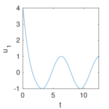
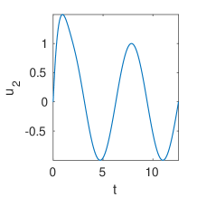
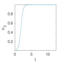
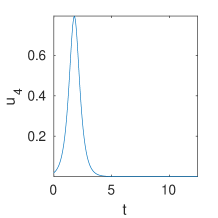
Figure 9: Canonical path from $(x_{1},x_{2})=(4,0)$ to $\hat{u}_{0}=(1,0,1,0)$ on CPS $\hat{u}$, $(\rho,\omega,\theta)=(1,1,1)$.

In cmds_advanced we essentially decrease $\omega$ (to $0.04$) which makes the problem more expensive due to slow convergence to $\hat{u}$, cf. (59). For $\omega=0.04$ we obtain $\gamma_{2}\approx 0.52$ for the leading stable multiplier. Intuitively, a change of $\omega$ correspond to a rescaling of time in the costates by $\frac{1}{\omega}$, i.e., small $\omega\ll 1$ reduces the speed of the costates. Then we expect that a canonical path spirals around the CPS several times while approaching it, and hence a long truncation time will be necessary for its computation. Figure 10(a) depicts typical results. We also compare the analytical and numerical Floquet multipliers, and generally find good agreement only for reasonably fine $t$–discretizations. In Fig. 10(b) we compare the deviation of the $x_{1}$–maxima of $u$ from $\hat{u}_{0,1}$ with the asymptotic analytical prediction, showing rather good agreement, see Cell 2 of cmds_advanced.

(a)	(b)	(c)

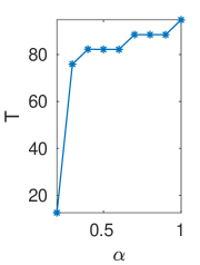
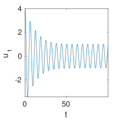
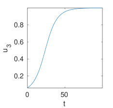
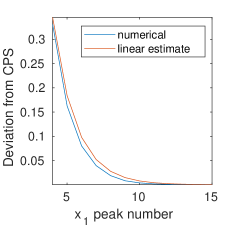
Figure 10: CP from states $(4,0)$ to $\hat{u}_{0}$ for $\omega=0.04$, yielding $\gamma_{2}\approx 0.52$ and hence slow convergence. (a) Adaptation of the truncation time $T$ during the continuation (initialized with $T=2T_{p}$). At $\alpha=0.3,0.4,0.7$ and $\alpha=1$ additional periods are added, while during the Newton loops $T$ only changes slightly. (b) $x_{1}=u_{1}$ and $y_{1}=u_{3}$ from the CP. (b) Deviation of the maxima of $u_{1}$ from $1$ (the maximum of $\hat{u}_{1}$) on the CPS (blue line), and deviation predicted by the leading stable multiplier (red line).

3.2 Optimal pollution mitigation

As an example for an OC problem with Hopf bifurcations we consider

$$V(v_{0}(\cdot))\stackrel{{\scriptstyle!}}{{=}}\max_{q(\cdot,\cdot)}J(v_{0}(\cdot),q(\cdot,\cdot)),\qquad J(v_{0}(\cdot),q(\cdot,\cdot)):=\int_{0}^{\infty}{\rm e}^{-\rho t}J_{ca}(v(t),q(t))\,{\rm d}t,$$ (60a)

with discount rate $$\rho>0 J_{ca}(v(\cdot,t),q(\cdot,t))=\frac{1}{|\Omega|}\int_{\Omega}J_{c}(v(x,t),q(x,t))\,{\rm d}x J_{c}(v,q)=pv_{1}-\beta v_{2}-C(q) C(q)=q+\frac{1}{2\gamma}q^{2}$$, and where as in §2.1 and §2.2 is the spatially averaged current value function, with here the local current value, . The state evolution is

$${\partial}_{t}v_{1}=-q+d_{1}\Delta v_{1},\quad{\partial}_{t}v_{2}=v_{1}-\alpha(v_{2})+d_{2}\Delta v_{2},$$ (60b)

with Neumann BCs ${\partial}_{\bf n}v=0$ on ${\partial}\Omega$, where $v_{1}=v_{1}(t,x)$ models the emissions of some firms, and $v_{2}=v_{2}(t,x)$ is the pollution stock, while the control $q=q(t,x)$ models the firms’ abatement policies. In $J_{c}$, $pv_{1}$ and $\beta v_{2}$ are the firms’ value of emissions and costs of pollution, and $C(q)$ are the costs for abatement, and $\alpha(v_{2})=v_{2}(1-v_{2})$ in (60b) is the recovery function of the environment. Again, the $\max$ in (60a) runs over all admissible controls $q$, meaning that $q\in L^{\infty}((0,\infty)\times\Omega,{\mathbb{R}})$, and we do not consider active control or state constraints. The associated ODE OC problem (no $x$–dependence of $v,q$) was set up and analyzed in [TW96, Wir00]; in suitable parameter regimes it shows Hopf bifurcations of periodic orbits for the associated canonical (ODE) system. See also, e.g., [DF91, HMN92, Wir96, KGF⁺02, GCF⁺08] for results about the occurrence of Hopf bifurcations and optimal periodic solutions in ODE OC problems.

Setting $D=\begin{pmatrix}d_{1}&0\\ 0&d_{2}\end{pmatrix}$, $g_{1}(v,q)=\begin{pmatrix}-q\\ v-\alpha(w)\end{pmatrix}$, and introducing the co–states (Lagrange multipliers)

$$\lambda:\Omega\times(0,\infty)\rightarrow{\mathbb{R}}^{2},$$

and the (local current value) Hamiltonian ${\cal H}={\cal H}(v,\lambda,q)=J_{c}(v,q)+\left\langle\lambda,D\Delta v+g_{1}(v,q)\right\rangle$, by Pontryagins Maximum Principle we obtain

$${\partial}_{t}v ={\partial}_{\lambda}{\cal H}=D\Delta v+g_{1}(v,q),\quad v|_{t=0}=v_{0},$$ (61a)

$${\partial}_{t}\lambda =\rho\lambda-{\partial}_{v}{\cal H}=\rho\lambda+g_{2}(v,\lambda)-D\Delta\lambda,$$ (61b)

where ${\partial}_{\bf n}\lambda=0$ on ${\partial}\Omega$, and

$$q=q(\lambda_{1})=-(1+\lambda_{1})/\gamma.$$ (62)

Finally we set $u(t,\cdot):=(v(t,\cdot),\lambda(t,\cdot)):\Omega\rightarrow{\mathbb{R}}^{4}$, and write (61) as

$${\partial}_{t}u=-G(u):={\cal D}\Delta u+f(u),$$ (63)

where $\displaystyle{\cal D}=$diag$(d_{1},d_{2},-d_{1},-d_{2})$, $\displaystyle f(u)=\biggl{(}-q,v_{1}-\alpha(v_{2}),\rho\lambda_{1}-p-\lambda_{2},(\rho+\alpha^{\prime}(v_{2}))\lambda_{2}+\beta\biggr{)}^{T}$.

For all parameter values, (63) has the spatially homogeneous CSS

$$u^{*}=(z_{*}(1-z_{*}),z_{*},-1,-(p+\rho)),\quad\text{where}\quad z_{*}=\frac{1}{2}\left(1+\rho-\frac{\beta}{p+\rho}\right).$$

We use similar parameter ranges as in [Wir00], namely

$$(p,\beta,\gamma)=(1,0.2,300),\text{ and }\rho\in[0.5,0.65]\text{ as a continuation parameter},$$ (64)

consider (63) over $\Omega=(-\pi/2,\pi/2)$, and set the diffusion constants to $d_{1}=0.001,d_{2}=0.2$.

Remark 3.1.

a) The motivation for the choice of $d_{1,2}$ is to have the first (for increasing $\rho$) Hopf bifurcation to a spatially patterned branch, and the second to a spatially uniform Hopf branch, because the former is more interesting from the PDE point of view. We use that the Hopf bifurcations for the model (63) can be analyzed by a simple modification of [Wir00, Appendix A]. We find that for branches with spatial wave number $l\in{\mathbb{N}}$ the necessary condition for Hopf bifurcation, $K>0$ from [Wir00, (A.5)], becomes $K=-(\alpha^{\prime}+d_{2}l^{2})(\rho+\alpha^{\prime}+d_{2}l^{2})-d_{1}l^{2}(\rho+d_{1}l^{2})>0$. Since $\alpha^{\prime}=\alpha^{\prime}(z_{*})<0$, a convenient way to first fulfill $K>0$ for $l=1$ is to choose $0<d_{1}\ll d_{2}<1$, such that for $l=0,1$ the factor $\rho+\alpha^{\prime}+d_{2}l^{2}$ is the crucial one.

b) Even though we do not specify the units, $\rho\in[0.5,0.65]$ may be considered quite large, in the following sense. Typical periods of the CPS will be between 20 and 40, and, moreover, CPs starting not close to these CPSs will need times scales $T\geq 100$ (and larger) for convergence to the CPSs, but $\rho>0.5$ means that the large time ($T\geq 100$) behavior of a CP hardly plays a role for the value of the CP, as the discounted current value drops to ${\rm e}^{-\rho t}J_{c}(t)<{\rm e}^{-50}$. Thus, our example turns out to be somewhat academic, but nevertheless it will show the robustness of our approach.

c) In the literature, most of the (ODE) OC examples with canonical periodic states show these at rather large discount rates, see, e.g., [HMN92, KGF⁺02]. An exception is for instance the resource management model in [BPS01], where (ODE) CPSs are found at discount rates near $\rho=0.1$. We have also implemented this example, including a PDE setting, but its main drawback, already hinted at in [BPS01], is that already in the ODE setting it is extremely rich in CPSs, which undergo several period doubling and fold bifurcations, and the smaller $\rho$ is again offset by rather long periods (between 20 and 60). In summary, we focus on the pollution example because it gives a clear and robust bifurcation picture. $\rfloor$

(a) spectrum of ${\partial}_{u}G(u^{*})$, $\rho=0.5$	(b) bifurcation diagram	(c) time series on h2/pt17 (spat. homogen. branch)
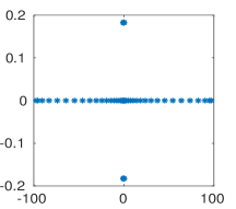
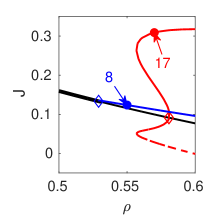
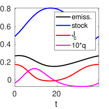
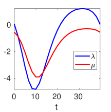
(d) sample plots at h1/pt8
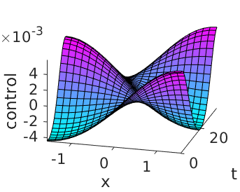
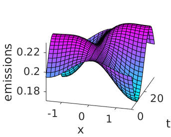
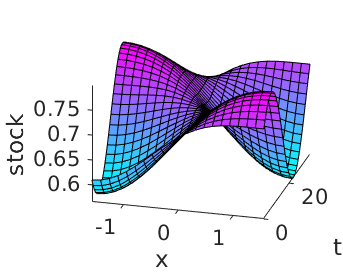
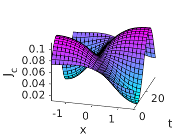
(e) the $\frac{n_{u}}{2}$ smallest $\gamma_{j}$ at h1/pt8	(f) $|\gamma_{j}|$ for the $\frac{n_{u}}{2}$ largest $\gamma_{j}$ at h1/pt8	(g) the $\frac{n_{u}}{2}$ smallest $\gamma_{j}$ at h1/pt10 and at h2/pt17

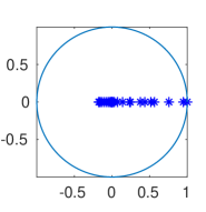
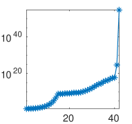
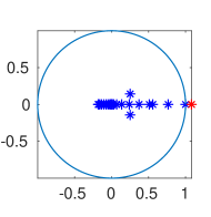
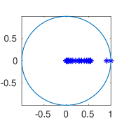
Figure 11: (a) full spectrum of the linearization of (63) around $u^{*}$ at $\rho=0.5$ on a coarse mesh with $n_{p}=21$. (b) Bifurcation diagram, value $J$ over $\rho$. Black: $u^{*}$; blue: h1, red: h2, $J(u^{H};0)$ (full line) and $J(u^{H};T/2)$ (dashed line). (c) Time series of a spatially homogeneous solution, including current value $J_{c}$, control $q$, and co–states $\lambda_{1,2}$. (d) Example plots of $u_{H}$ at h1/pt8. (e)-(g) Floquet multipliers at selected CPS, with $\rho=0.56$ at h1/pt10. The largest $\gamma$ in (f) is $\gamma_{84}\approx 10^{79}$.

The implementation of (63) works as usual, and, moreover, the computation of the bifurcation diagram of CSS and CPS, and of the Floquet multipliers, is already explained in [Uec19a, Uec19c], and the novelty here is the computation of CPs to the CPSs in a full PDE setting. Table 7 gives a few comments on the used files. In Figure 11 (essentially already contained in [Uec19a]) we give some basic results for (63) with a coarse spatial discretization of $\Omega$ by only $n_{p}=21$ points (and thus $n_{u}=84$). (a) shows the full spectrum of the linearization of (63) around $u^{*}$ at $\rho=0.5$. (b) shows a basic bifurcation diagram. At $\rho=\rho_{1}\approx 0.53$ there bifurcates a Hopf branch h1 with spatial wave number $l=1$, and at $\rho=\rho_{2}\approx 0.58$ a spatially homogeneous ($l=0$) Hopf branch h2 bifurcates subcritically with a fold at $\rho=\rho_{f}\approx 0.56$. (c) shows the pertinent time series on h2/pt17. As should be expected, $J_{c}$ is large when the pollution stock is low and emissions are high, and the pollution stock follows the emissions with some delay. In (b) we plot $J$ over $\rho$. For the CSS $u^{*}$ this is again simply $J(u^{*})=\frac{1}{\rho}J_{c,a}(u^{*})$, but for the periodic orbits we take into account the phase, which is free for (63). If $u_{H}$ is a $T_{p}$ periodic solution of (63), then, for $\phi\in[0,T_{p})$, we consider

$$J(u_{H};\phi):=\int_{0}^{\infty}{\rm e}^{-\rho t}J_{c,a}(u_{H}(t+\phi))\,{\rm d}t=\frac{1}{1-{\rm e}^{-\rho T_{p}}}\int_{0}^{T_{p}}{\rm e}^{-\rho t}J_{c,a}(u_{H}(t+\phi))\,{\rm d}t,$$

which in general may depend on the phase, and for h2 in (c) we plot $J(u_{H};\phi)$ for $\phi=0$ (full red line) and $\phi=T/2$ (dashed red line). For the spatially periodic branch h1, $J_{c,a}(t)$ averages out in $x$ and hence $J(u_{H};\phi)$ only weakly depends on $\phi$. Thus, we first conclude that for $\rho\in(\rho_{1},\rho_{f})$ the spatially patterned periodic orbits from h1 give the highest $J$, while for $\rho\geq\rho_{f}$ this is obtained from h2 with the correct phase. The example plots (d) at h1/pt8 illustrate the spatio-temporal dependence of $q$, $v$, and $J_{c}$ on the patterned CPS.

bdcmds,cpcmds	bifurcation diagram of CSS and CPS, and computation of some CPs
cpplot, polldiagn	plot of CPs, computation and plotting of diagnostics for CPs.

Table 7: Main scripts and functions in ocdemos/pollution. Additionally, we locally modify some standard pde2path functions for convenience (plotting).

It remains to

• compute the defects $d(u^{*})$ of the CSS and $d(u_{H})$ of periodic orbits on the bifurcating branches,

• compute CPs to saddle point CSSs and CPSs.

For $d(u^{*})$ we find that it starts with $0$ at $\rho=0.5$, and, as expected, increases by 2 at each Hopf point. Below we shall focus on CPs to the CPSs h1/pt8 and h2/pt17, and in Fig. 11(e–g) we illustrate typical multiplier spectra, computed with pqzschur, which yields $|\gamma_{1}-1|<10^{-8}$ for all computations, i.e., a very accurate trivial multiplier, and hence we trust it. The large multipliers are very large, i.e., $10^{40}$ and larger, even for the coarse space discretization, as should be expected from the spectrum in Fig. 11(a).

On h1 we find $d(u_{H})=0$ up to pt9, see (e) for the $n_{u}/2$ smallest multipliers at pt8, and (f) for $|\gamma_{j}|$ for the large ones, which are mostly real. For larger $\rho$ the h1 branch looses stability by a (second) multiplier going through 1, and in fact at h1/pt8 we have $\gamma_{2}\approx 0.948$, which suggests a slow convergence of CPs to the CPS. On h2 we start with $d(u_{H})=3$, but $d(u_{H})=0$ after the fold until $\rho=\rho_{1}\approx 0.6$, after which $d(u_{H})$ increases again by multipliers going though 1. At pt17 we have $\gamma_{2}\approx 0.905$, again suggesting slow convergence.

Nevertheless, the computation of CPs (from various initial states) to the CPSs works quite robustly, and in Fig. 12 we present some sample results from cpcmds, and from pollODE/cpcmdsode, which treats the same problem as an ODE. The idea is that the behavior of the spatially homogeneous CPs can be studied much faster in the ODE setting due to much less DoF. Also, for instance the ODE multipliers $\gamma$ at h2/pt17 are $\gamma\approx(0.303,\ 1,\ 1.012*10^{10},\ 3.789*10^{10})$, i.e., $\gamma_{2}=0.303$. The associated ODE paths then also exist in the PDE as spatially homogeneous paths, and show the same convergence behavioras long as the instability which yields the existence of the patterned CPS h1 plays no role.

In Fig. 12(a)–(d) we show CPs to the CSS at $\rho=0.55$ (starting from two different initial states), and to the homogeneous CPS h2/pt17 at $\rho=0.57$. The convergence to the CSS is very slow as we are close to the Hopf bifurcation and hence the slowest decay rate is $\mu=0.0059$. For $(v_{0},w_{0})=(0.4,0.4)$ (significant initial emissions and pollution) we obtain a negative value $J\approx-0.1297$, as initially the emission are strongly reduced and the initial abatement investments are high. For $(v_{0},w_{0})=(0,0)$ (no initial emissions and pollution) we have $J\approx 0.0202$ due to increasing initial emission and negative initial abatement investments. To compute CPs to the CPS, we start with a rather small $T=2T_{p}$ and for $\|u(1)-\hat{u}_{0}\|>\varepsilon_{\infty}=10^{-2}$ use the extension of the CP by copies of the CPS during the continuation in $\alpha$. This leads to the extension of $T$ to about $10T_{p}$, and to $\|u(1)-\hat{u}_{0}\|_{\infty}\approx 10^{-4}$ for the final deviation from the target $\hat{u}_{0}$, and we also illustrate how to a posteriori decrease this deviation to $10^{-6}$. We also run a few further tests, for instance computing CPs from the same ICs to shifted CPSs, e.g., h2 shifted by half a period. As expected, shifting the base point $\hat{u}_{0}$ on the CPS just expands or shortens the truncation time $T$ by half a period, see Fig. 12(d).

(a)	(b)	(c)	(d)

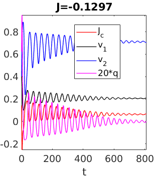
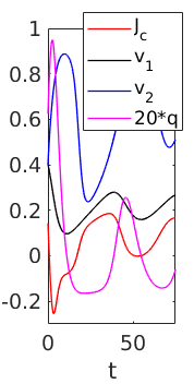
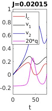
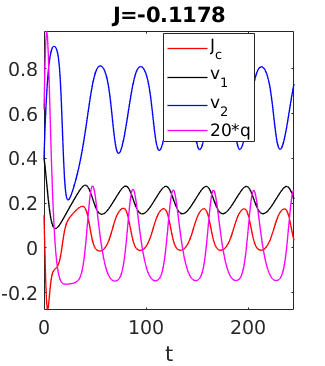
(e)

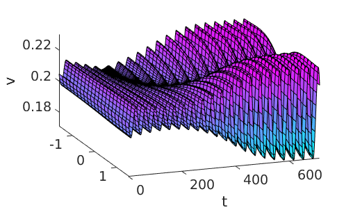
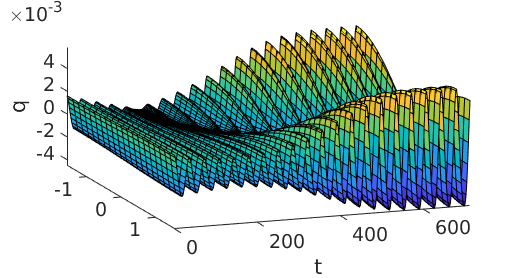
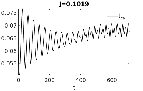
Figure 12: CPs to the CSS and to different CPS from different initial states. (a,b) CPs to the CSS at $\rho=0.55$, ICs $v\equiv(0.4,0.4)$ in (a), with zoom of the initial phase on the right, and ICs $v\equiv(0,0)$ in (b) showing the different initial behavior, and hence a different value. (c) CP to the homogeneous CPS at $\rho=0.57$, ICs $v\equiv(0.4,0.4)$. (d) Same as (c), but with different target $\hat{u}_{0}$ on the CPS (phase shift by half a period). In (b–d) we start with a short initial $T=2T_{p}$ and set $\varepsilon_{\infty}=10^{-2}$, leading to repeated extension of the CPs by the CPS $\hat{u}$ via (42). (e) CP to the patterned CPS h1/pt8 at $\rho=0.56$, starting close ($\alpha=0.975$) to the states $v\equiv(0.205,0.72)$ which is near the CSS at $\rho=0.56$. The patterning instability of the CSS then only manifests after a rather long transient. See text for further discussion.

In Fig. 12(e) we give one exemplary CP to the inhomogeneous CPS at $\rho=0.56$, starting with ICs $0.975*(0.21,0.71)+0.025*\hat{u}_{0}$. The ICs are thus quite close to the CSS, which is stable in the ODE, but (very weakly) unstable in the PDE, as we are beyond the primary Hopf bifurcation. Consequently, the associated CP transiently decays towards the CSS, before the inhomogeneous instability manifests and the CP converges to the inhomogeneous CPS. In summary, these examples show that our algorithms allow a robust control towards CSSs and CPSs with the SPP.

4 Summary and outlook

We explained how to study OC problems of class (1) in pde2path. The class (1) is quite general, and with the pde2path machinery we have a powerful tool to first study the bifurcations of CSS/CPS. For the computation of canonical paths to CSSs and CPSs, our Algorithms 1 and 2 implement for the class (1) variants of the connecting orbits methods explained for ODE problems in [GCF⁺08, Chapter 7]. For the CPS case, because of the very small and very large mutipliers present due diffusion and anti–diffusion, an important technical issue is the use of pqzschur to compute the projection onto the center–unstable eigenspace. Similarly, the idea to start with a rather small truncation time $T$ and then using (42), i.e., adding copies of the CPS to the CP to ensure convergence, seems crucial to have a fast and robust algorithm.

There also is a number of issues we do not address (yet), for instance inequality constraints that frequently occur in OC problems. In our examples we can simply check the natural constraints (such as $v,q\geq 0$ in the sloc example) a posteriori and find them to be always fulfilled, i.e., inactive. If such constraints become active the problem becomes much more complicated.

References

- [AAC11] S. Aniţa, V. Arnăutu, and V. Capasso. An introduction to optimal control problems in life sciences and economics. Birkhäuser/Springer, New York, 2011.
- [Bey90] W.-J. Beyn. The numerical computation of connecting orbits in dynamical systems. IMA J. Numer. Anal., 10(3):379–405, 1990.
- [BPS01] W.J. Beyn, Th. Pampel, and W. Semmler. Dynamic optimization and Skiba sets in economic examples. Optimal Control Applications and Methods, 22(5–6):251–280, 2001.
- [BX08] W.A. Brock and A. Xepapadeas. Diffusion-induced instability and pattern formation in infinite horizon recursive optimal control. Journal of Economic Dynamics and Control, 32(9):2745–2787, 2008.
- [BX10] W. Brock and A. Xepapadeas. Pattern formation, spatial externalities and regulation in coupled economic–ecological systems. Journal of Environmental Economics and Management, 59(2):149–164, 2010.
- [DCF+97] E. Doedel, A. R. Champneys, Th. F. Fairgrieve, Y. A. Kuznetsov, Bj. Sandstede, and X. Wang. AUTO: Continuation and bifurcation software for ordinary differential equations (with HomCont). http://indy.cs.concordia.ca/auto/, 1997.
- [DF91] E. Dockner and G. Feichtinger. On the optimality of limit cycles in dynamic economic systems. Journal of Economics, 53:31–50, 1991.
- [DKvVK08] E. J. Doedel, B. W. Kooi, G. A. K. van Voorn, and Yu. A. Kuznetsov. Continuation of connecting orbits in 3D-ODEs. I. Point-to-cycle connections. Internat. J. Bifur. Chaos Appl. Sci. Engrg., 18(7):1889–1903, 2008.
- [DKvVK09] E. J. Doedel, B. W. Kooi, G. A. K. van Voorn, and Yu. A. Kuznetsov. Continuation of connecting orbits in 3D-ODEs. II. Cycle-to-cycle connections. Internat. J. Bifur. Chaos Appl. Sci. Engrg., 19(1):159–169, 2009.
- [dWDR+18] H. de Witt, T. Dohnal, J.D.M. Rademacher, H. Uecker, and D. Wetzel. pde2path - Quickstart guide and reference card, 2018.
- [GCF+08] D. Grass, J.P. Caulkins, G. Feichtinger, G. Tragler, and D.A. Behrens. Optimal Control of Nonlinear Processes: With Applications in Drugs, Corruption, and Terror. Springer, 2008.
- [Gra15] D. Grass. From 0D to 1D spatial models using OCMat. Technical report, ORCOS, 2015.
- [GU17] D. Grass and H. Uecker. Optimal management and spatial patterns in a distributed shallow lake model. Electr. J. Differential Equations, 2017(1):1–21, 2017.
- [GUU19] D. Grass, H. Uecker, and T. Upmann. Optimal fishery with coastal catch. Natural Resource Modelling, (e12235), 2019.
- [HMN92] R. F. Hartl, A. Mehlmann, and A. Novak. Cycles of fear: periodic bloodsucking rates for vampires. J. Optim. Theory Appl., 75(3):559–568, 1992.
- [KGF+02] P. Kort, A. Greiner, G. Feichtinger, J Haunschmied, A. Novak, and R. Hartl. Environmental effects of tourism industry investments: an inter‐temporal trade‐off. Optim. Control – Appl. and Methods, 23(1):1–19, 2002.
- [Kre01] D. Kressner. An efficient and reliable implementation of the periodic qz algorithm. In IFAC Workshop on Periodic Control Systems. 2001.
- [KW10] T. Kiseleva and F.O.O. Wagener. Bifurcations of optimal vector fields in the shallow lake system. Journal of Economic Dynamics and Control, 34(5):825–843, 2010.
- [MS02] F. Mazzia and I. Sgura. Numerical approximation of nonlinear BVPs by means of BVMs. Applied Numerical Mathematics, 42(1–3):337–352, 2002. Numerical Solution of Differential and Differential-Algebraic Equations, 4-9 September 2000, Halle, Germany.
- [MST09] F. Mazzia, A. Sestini, and D. Trigiante. The continuous extension of the B-spline linear multistep methods for BVPs on non-uniform meshes. Applied Numerical Mathematics, 59(3–4):723–738, 2009.
- [MT04] F. Mazzia and D. Trigiante. A hybrid mesh selection strategy based on conditioning for boundary value ODE problems. Numerical Algorithms, 36(2):169–187, 2004.
- [Pam01] Th. Pampel. Numerical approximation of connecting orbits with asymptotic rate. Numerische Mathematik, 90(2):309–348, 2001.
- [RU18] J.D.M. Rademacher and H. Uecker. The OOPDE setting of pde2path – a tutorial via some Allen-Cahn models, 2018.
- [RZ99a] J. P. Raymond and H. Zidani. Hamiltonian Pontryagin’s principles for control problems governed by semilinear parabolic equations. Appl. Math. Optim., 39(2):143–177, 1999.
- [RZ99b] J. P. Raymond and H. Zidani. Pontryagin’s principle for time-optimal problems. J. Optim. Theory Appl., 101(2):375–402, 1999.
- [Ski78] A. K. Skiba. Optimal growth with a convex-concave production function. Econometrica, 46(3):527–539, 1978.
- [Tau15] N. Tauchnitz. The Pontryagin maximum principle for nonlinear optimal control problems with infinite horizon. J. Optim. Theory Appl., 167(1):27–48, 2015.
- [Trö10] Fredi Tröltzsch. Optimal control of partial differential equations, volume 112 of Graduate Studies in Mathematics. American Mathematical Society, Providence, RI, 2010.
- [TW96] O. Tahvonen and C. Withagen. Optimality of irreversible pollution accumulation. Journal of Environmental Economics and Management, 20:1775–1795, 1996.
- [Uec16] H. Uecker. Optimal harvesting and spatial patterns in a semi arid vegetation system. Natural Resource Modelling, 29(2):229–258, 2016.
- [Uec19a] H. Uecker. Hopf bifurcation and time periodic orbits with pde2path – algorithms and applications. Comm. in Comp. Phys, 25(3):812–852, 2019.
- [Uec19b] H. Uecker. User guide on Hopf bifurcation and time periodic orbits with pde2path, 2019. Available at [Uec19d].
- [Uec19c] H. Uecker. User guide on Hopf bifurcation and time periodic orbits with pde2path, 2019.
- [Uec19d] H. Uecker. www.staff.uni-oldenburg.de/hannes.uecker/pde2path, 2019.
- [UWR14] H. Uecker, D. Wetzel, and J.D.M. Rademacher. pde2path – a Matlab package for continuation and bifurcation in 2D elliptic systems. NMTMA, 7:58–106, 2014.
- [Wir96] Fr. Wirl. Pathways to Hopf bifurcation in dynamic, continuous time optimization problems. Journal of Optimization Theory and Applications, 91:299–320, 1996.
- [Wir00] Fr. Wirl. Optimal accumulation of pollution: Existence of limit cycles for the social optimum and the competitive equilibrium. Journal of Economic Dynamics and Control, 24(2):297–306, 2000.