Abstract

We describe by means of some examples how some functionality of the mesh adaptation package trullekrul can be used in pde2path.

1 Introduction

The Matlab package pde2path [UWR14, Uec19c] is designed for numerical continuation and bifurcation analysis of systems of PDEs of the form

$$M{\partial}_{t}u=\nabla\cdot(c\otimes\nabla u)-au+b\otimes\nabla u+f,$$ (1)

where $u=u(x,t)\in{\mathbb{R}}^{N}$, $t\geq 0$, $x\in\Omega$, $\lambda\in{\mathbb{R}}^{p}$ is a parameter vector, $M\in{\mathbb{R}}^{N\times N}$ is a mass matrix, which may be singular, and the coefficients $c,a,b$ and $f$ may depend on $x,\lambda$ and $u$. Details on the terms in (1), the discretization of (1) by the FEM, the boundary conditions associated to (1), and how to use pde2path to compute branches of steady and time periodic solutions of (1), can be found in [RU19, Uec19b, Uec19a] and some further tutorials which together with the software and demos can be downloaded at [Uec19c].

Here we explain how to use the anisotropic mesh adaptation package trullekrul [JG16, Jen17] in pde2path. For this we extend the introductory tutorial [RU19] by a number of some advanced examples for steady Allen–Cahn type problems, i.e., problems of type

$$G(u):=-c\Delta u+f(u),\quad u=u(x)\in{\mathbb{R}},\quad x\in\Omega\subset{\mathbb{R}}^{d}\text{ a bounded domain},$$ (2)

with diffusion constant $c$, ’nonlinearity’ (everything except diffusion) $f:{\mathbb{R}}\to{\mathbb{R}}$ (which also depends on parameters). For $\Omega$ we shall restrict to rectangles (2D, $d=2$) and cuboids (3D, $d=3$), and $f$ and the boundary conditions will be given for the specific examples below.

In [RU19] we also explain some settings for mesh adaptation for problems of type (2) based on mesh refinement using standard a posteriori error estimators, in 1D and 2D. In the context of solution branches $s\mapsto(u(s),\lambda(s))$ for (2) as computed by the main user–interface routine cont of pde2path, where $\lambda$ is used as a symbol for the active continuation parameter, it is desirable to adapt the mesh during continuation, for instance after a number of continuation steps, or if the error estimate is above some user given threshhold. This mesh adaptation so far has been done in pde2path in a simple ad hoc way: first we coarsen the current mesh to a given (essentially fixed and uniform) background mesh by interpolation of the current solution to the background mesh, and then generate a new mesh by refining the coarse mesh and solution. The coarsening is necessary because otherwise we may end up with (at places) unnessarily fine meshes. However, the simple approach sketched above is not very efficient, may lead to undesired branch–switching after coarsening, and, moreover, has so far not been fully implemented in 3D. By interfacing pde2path with trullekrul, we now have genuine 2D and 3D adaptation options during continuation of branches, which means coarsening (only) where appropriate together with moving of mesh–points and refinement.

In §2 we explain the general setup of trullekrul in pde2path, based on the standard data structures of pde2path with all data stored in the struct p, i.e., function handles to the rhs of (11a) and its Jacobian, FEM mesh, file-names for saving, controls for plotting, numerical constants such as stepsizes and solution tolerances), and the solution p.u itself and the current tangent to the solution branch. For this background, the pde2path data structures, the continuation algorithms, and the general usage of pde2path, we refer to [dWDR⁺19] and the tutorials at [Uec19c], in particular [RU19]. In §3 we then explain the usage of trullekrul by some example problems of type (11a).

2 General setup of trullekrul in pde2path

Given a function $u:\Omega\to{\mathbb{R}}$, trullekrul aims to optimize the FEM mesh to minimize the interpolation error $\|u-u_{h}\|_{L^{p}(\Omega)}$, where $u_{h}$ as usual is the continuous piecewise linear interpolation of the nodal values. This is based on the discrete Hessian $H(u_{h})$ of $u_{h}$, and the associated metric field

$$\Psi=\frac{1}{\eta}(\det(\widetilde{H}))^{-\frac{1}{2p+d}}\widetilde{H},$$ (3)

where $\widetilde{H}$ denotes a matrix of absolute values of the eigenvalues of $H(u_{h})$, and $\eta$ is a scaling factor, which can be used to control the number of mesh points. In [CSX07] it is shown that meshes that are uniform wrt to $\Psi$ minimize $\|u-u_{h}\|_{L^{p}(\Omega)}$. Thus, using $\Psi$, edge lengths $L_{\text{elem}}$ of the triangulation are computed wrt to the metric $\Psi$, and then elements are coarsened/refined according to the following algorithm (cf. [LSB05, Fig.6]):

Compute the maximum edge length $L_{\text{max}}$ in metric space, and perform the following loop until $L_{\text{max}}<L_{\text{up}}$ or until it=imax: 1. Eliminate the edges shorter than $L_{\text{low}}$ by coarsening the respective elements; this includes swapping of elements with wrong orientation. 2. Refine the elements with $L_{\text{elem}}>L_{\text{up}}$ by splitting their longest edge and postprocessing (splitting of adjacent elements); 3. Move mesh–points according to a smoothing algorithm based on the (discrete) Laplacian. 4. Update $\Psi,\widetilde{H}$ and hence $L_{\text{elem}}$ and $L_{\text{max}}$.

Algorithm 2.1: Outline of trullekrul mesh adaptation. Given a current solution $u_{h}$, the inner adaptation loop is performed, and the resulting new $u_{h}$ is used as an initial guess for a Newton loop on the new mesh. This outer step is repeated p.nc.ngen times.

The details of each of the steps 1 to 3 in Algorithm 2.1 are controlled by a number of trullekrul parameters, which in pde2path we store in the field p.trop (trullekrul options) of the basic data struct p. To initialize trop we provide the two functions troptions2D and troptions3D, which as variants of the trullekrul function gen_options set trullekrul parameters in the way which appear to be most robust and efficient in 2D, respectively 3D. For us, the most important parameter is $\eta$ in (3), where, for fixed $L_{\text{up}}$, larger $\eta$ gives less triangles to refine. For adaptation during continuation we typically want to keep the number of mesh points $n_{p}$ below some bound, and thus $\eta$ should be set by some function which depends on $n_{p}$. To give maximum flexibility, the user may provide such a function in trop.etafu with signature eta=etafu(p,np). The default setting is trop.etafu=@stanetafu, which returns the constant $\eta=10^{-3}$, while a simple dependence on $n_{p}$ is given by eta=etafua(p,np) which (by default) returns $10^{-5}{\tt np}$. Altogether, in Table 1 we list the trop parameters/function handles which we find most useful for tuning the adaptation, and we strongly recommend to experiment with these and the other trullekrul parameters, see the sources for detailed comments. The pde2path parameter to switch on mesh–adaptation by trullekrul instead of option (i) within cont is p.sw.trsw$>0$.

Table 1: Most important parameters/function handles in p.trop, see also troptions2D and troptions3D for further parameters and comments. p.trcop (see below) needs the same parameters as p.trop, and additionally p.trcop.sw, see bottom of table. Typically, we just copy trop to trcop, set p.trcop.npb, and reset selected parameters such as p.trcop.sw.

Parameter	meaning, default value
etafu	default eta=stanetafu(p,np) returning 0.001. Larger eta gives less elements to adapt. See also etafua, yielding $\eta=10^{-5}n_{p}$, and we recommend to copy etafua to the local directory and experiment with the prefactor.
zfu	function handle with signature z=zfu(p), to select the field $u$ for which the interpolation error is estimated. Default zfu=@stanzfu for which $z=u_{1}$ (first component of current solution). May be useful to overload for multi–component systems. In some cases, also scaling of $z$ is useful, e.g., $z=\exp(u_{1})$.
setids	function handle needed to link the pde2path data structures with trullekrul in case that different boundary segment numbers (and different BCs on different segments) are assigned in pde2path. Defaults: @setidssq in 2D (corresponding to a rectangular domain, as also used in stanpdeo2D); @setidsbar in 3D (corresponding to a cuboid domain, as also used in stanpdeo3D).
sw	behavior of tradapt according to Table 2; default 15.
ppar	$p$ to optimize the interpol. error in the $p$-norm metric. Default: 1000, i.e., close to $\infty$ norm.
innerit	number of iterations in trullekrul, default 2. (Not to confuse with p.nc.ngen giving the ’outer’ number of adaptation iterations).
Llow, Lup	lower/upper thresholds for edges in metric space, defaults $1/\sqrt{2}$ and $\sqrt{2}$. Smaller Llow can be used to avoid too much coarsening.
qualP	weight for combining mesh qualtity in metric space and euclidean space. Defaults: 0 in 2D (metric space only), 2 in 3D (avoiding too acute tetrahedra)
trcop.npb	desired number of mesh-points for pure coarsening steps.
trcop.crmax	maximum number of pure coarsening steps.

In some examples (in particular in 3D, see below), it is useful for mesh adaptation within cont to first use only the coarsening and moving functionality of trullekrul, and then adapt again with refinement. For this two step approach we provide a modification of the main trullekrul wrapper function adapt_mesh, named tradapt. Both, adapt_mesh and tradapt, take the option field trop as last argument, and for tradapt this should contain the field trop.sw which encodes the operations

(face or edge) swapping, coarsening, moving (of mesh points), and refinement, (4)

in a binary way according to Table 2. Thus, coarsening and moving as a preparatory step before adaptation is encoded as p.trcop.sw=5, and additionally p.trcop.npb should contain the desired maximum number of meshpoints.

Table 2: Control of tradapt via sw based binary coding with the 1st/2nd/3rd/4th bit switching on moving/refinement/coarsening/swapping, abbreviated as m/r/c/s, respectively. sw=15 thus corresponds to the original trullekrul adapt_mesh behaviour.

sw	0	1	2	3	4	5	6	7	8	9	10	11	12	13	14	15
action	none	m	r	m,r	c	c,m	c,r	c,r,m	s	m,s	r,s	m,r,s	c,s	c,m,s	c,r,s	c,r,m,s

3 Example implementations and results

To illustrate the use and performance of the trullekrul mesh adaptation we discuss some demos from pdepath/acsuite, which also collects the demos discussed in [RU19], and again we stress that new users should at least briefly browse [RU19, §4] and the associated demos.

3.1 2D

Extending ac2D from [RU19].

We start with (2) on the rectangle $\Omega=(-2\pi,2\pi)\times(-\pi,\pi)$, with Dirichlet BC, i.e.

$$G(u):=-c\Delta u-\lambda u-u^{3}+\gamma u^{5}=0\text{ in $\Omega$},$$ (5a)

$$\text{$u=d\cos(y/2)$ on $\Gamma_{2}:=\{x=2\pi\}$, parameter $d$, and $u=0$ on ${\partial}\Omega\setminus\Gamma_{2}$}.$$ (5b)

The label $\Gamma_{2}=\{x=2\pi\}$ is due to the pde2path convention that the boundaries of rectangles as generated by stanpdeo2D have the order bottom–right–top–left. For $d=0$, (11) features the bifurcation points

$$\lambda_{jl}=(j/4)^{2}+(l/2)^{2},\ \ \phi_{jl}=\sin(j(x+2\pi)/4)\sin(l(y+\pi)/2),\ \ j,l=1,2,\ldots$$ (6)

from the trivial branch $u\equiv 0$. The associated bifurcating branches have already been discussed in [RU19, §4.1] and are computed in ac2D/cmds1. In ac2D/cmds2 we redo some of these computations starting with a very coarse mesh and aiming to illustrate the use and performance of trullekrul. Some results are shown in Fig. 3.1, which compares the older mesh adaptation by error estimators with that by trullekrul, for the solution on the first nontrivial branch at $\lambda=4$ (see (a)). Clearly, e2rs in (b) correctly identifies the triangles that are reasonable to refine, but refining the longest edges in Euclidean metric gives poor approximations at the ’boundary layers’. (c) shows a ’standard’ refinement of (a) by adapt_mesh from trullekrul (with the given parameters from troptions2D), and (d) shows a refinement of (a) by tradapt with sw=3, i.e., without coarsening (and without swapping). This gives significantly more mesh points than (c), and our main purpose here is to illustrate the a–posteriori coarsening of (d) in (e,f), which gives a rather similar mesh as in (c).

hu,ho

sl

(a) Original mesh, $n_{p}{=}264$	(b) e2rs refinement, $n_{p}{=}1200$	(c) trullekrul, $n_{p}{=}892$
(d) no coarsening, $n_{p}{=}1616$	(e) a-posteriori coarsening $n_{p}{=}879$	(f) top view of (d)

Selection of plots generated in ac2D/cmds2.m, illustrating different options for mesh-adaptation, see text for comments.

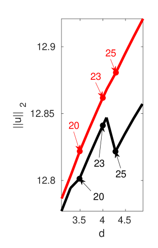
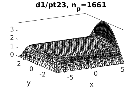
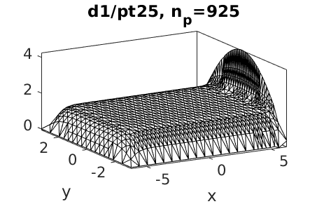
(a)	(b) simple adaptation (c) trullekrul adaptation

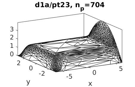
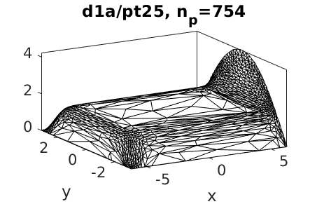
Figure 1: Further results from cmds2. Mesh adaptation every 5 steps of continuation in $d$, using e2rs and trullekrul, starting with the coarse mesh/solution from Fig. 3.1(a). See text for further comments.

Coarsening steps as in Fig. 3.1 from (d) to (e) are in particular useful for mesh adaptation during continuation. In Fig. 1 we continue the solution from Fig. 3.1(a) (at $\lambda=4$ and $d=0$) in $d$ with mesh adaption each 5th continuation step, again comparing mesh adaptation by trullekrul with the old ad hoc adaptation by coarsening to the background mesh and then refining. The black branch in (a) belongs to the old option. The meshes and solutions (see (b) for two example plots) generally appear reasonable, but for larger $d$ the interpolation down to the coarse background mesh and subsequent refinement become problematic, i.e., both appear somewhat underresolved at the $x=2\pi$ boundary. A typical sign for such problems due to an inadequate background mesh are jumps in the branch data at adaption, that in (a) start to appear on the black branch for $d>3$. The controlled coarsening–refine approach by trullekrul (red branch in (a)) is more robust in this respect. Of course, this is just one example, but it indicates a general result: if solutions during continuation develop boundary layers, or become strongly localized in some sense, use the trullekrul mesh adaptation. Listing 1 shows some pertinent commands for this for easy review.

⬇

%% ac2D cmds2; mesh-ada via oopde and trullekrul, initialize with very coarse mesh

p=[]; par=[1 -0.2 1 0]; % parameters [c lambda gamma d]

lx=2*pi; ly=pi; sw.ref=0; sw.sym=1; p=acinit(p,lx,ly,19,par,sw);

p.nc.ilam=2; p.nc.lammax=5; p.sol.ds=0.1; p.nc.dsmax=0.2;

46p=setfn(p,’trc’); p.plot.pstyle=1; p.usrlam=[2 4]; plotsol(p);

%% find first 3 BPs via findbif

p=findbif(p,3);

%% switch to first 3 bifurcating branches and continue

p=swibra(’trc’,’bpt1’,’c1’,0.1); p=cont(p);

51p=swibra(’trc’,’bpt2’,’c2’,0.1); p=cont(p);

p=swibra(’trc’,’bpt3’,’c3’,0.1); p=cont(p);

%% mesh-ada-OOPDE, yielding np=1220, nt=2366

trullem/ac2D/cmds2.m

Listing 1: Commands from ac2D/cmds2.m for continuation in $d$ with mesh adaptation by trullekrul.

A wandering boundary spot.

In a second example we consider (2) on the rectangle $\Omega=(-2\pi,2\pi)\times(-\pi,\pi)$ with the BCs

$$\left\{\begin{array}[]{l}\text{$u=\exp(-(x-\xi)^{2}-z^{2})$ on $\Gamma_{3}=\{y=\pi\}$, parameter $\xi$,}\\ \text{$u=0$ on $\Gamma_{1}=\{y=-\pi\}$, }\\ \text{${\partial}_{n}u=0$ on ${\partial}\Omega\setminus(\Gamma_{1}\cup\Gamma_{3})$. }\end{array}\right.$$ (10)

The purpose is to illustrate the mesh adaptation during continuation by considering a ’wandering spot’ (upon continuation in $\xi$) on the top boundary. Additionally, this gives the opportunity to show how to put a parameter into the assembling of boundary values. The demo directory is ac2Dwspot, and Listing 2 shows the implementation of the rhs $G$, where we need to assemble the BCs in each step.

⬇

function r=sGws(p,u) % wandering boundary spot, parameter dependent BCs

par=u(p.nu+1:end); u=u(1:p.nu); xi=par(4); gr=p.pdeo.grid;

bc1=gr.robinBC(0,0); bc3=gr.robinBC(1,0); % Neumann and DBC

bcs=[’exp(-(x-’ mat2str(xi) ’).^2)’]; % parameter dependent BCs

46bc2=gr.robinBC(1,bcs); gr.makeBoundaryMatrix(bc3,bc1,bc2,bc1);

[Q,Gbc,~,~]=p.pdeo.fem.assemb(gr); % the BC matrices

f=par(2)*u+u.^3-par(3)*u.^5; % the ’nonlinearity’

r=par(1)*p.mat.K*u-p.mat.M*f+p.nc.sf*(Q*u-Gbc); % the residual

Listing 2: ac2Dwspot/sGws.m, $G$ for the wandering spot example. Due to the $\xi$ dependence, here we need to assemble the BCs $G_{\text{BC}}$ in every call.

Fig. 2 (see also Listing 4) shows a continuation in $\xi$ in the subcritical case ($\lambda=-0.25$), where the solutions are essentially characterized by the position of the boundary spot. For illustration we aim at rather coarse meshes, set amod=5 (mesh-adaptation every 5th step), and allow for extra coarsening steps in trullekrul. The BD in (a) shows that this yields a reasonably smooth branch, and the sample plots in (b) that (as expected) the finest mesh may slighty lag behind the spot position (see in particular pt16), but otherwise the coarsening/refinement setup works very well.

⬇

%% 2DAC, wandering spot

p=[]; lx=2*pi; ly=3*pi/2; nx=7; sw.sym=1; sw.ref=1;

21par=[0.5 -0.25 1 -lx-0.1]; p=acinit(p,lx,ly,nx,par,sw);

p.nc.ilam=4; p.sol.ds=0.1; p.nc.dsmax=0.5; p=setfn(p,’ws0’);

p.sw.verb=2; p.sw.spcalc=1; p.sw.bifcheck=2; p.nc.lammax=lx+1;

p.fuha.sG=@sGws; p.fuha.sGjac=@sGwsjac; p.usrlam=-lx;

trullem/ac2Dwspot/cmds1.m

Listing 3: Selection from ac2Dwspot/cmds1.m. Continuation in $\xi$, $\lambda=-0.25$ (subcritical case).

(a)	(b)

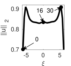
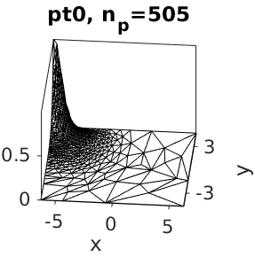
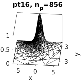
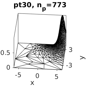
Figure 2: Example results from cmds1.m for (2) with the BCs 10, $(c,\lambda,\gamma)=(0.5,-0.25,1)$, continuation in $\xi$, with mesh–adapation every 5th step.

In cmds2.m we then continue in $\lambda$ at fixed $\xi=0$. The black branch in (a) initially corresponds to the ’trivial’ branch on which solutions are as in Fig. 2 (specifically pt16 at $\xi=0$). Continuation in $\lambda$ then yields an imperfect bifurcation to the primary unimodal branch in (a). Moreover, there are two BPs on the black branch, connected by the red branch. Alltogether, the trullekrul mesh adaptation with amod=10 yields robust results with still rather coarse meshes.

⬇

1%% continue soln at xi=0 in lambda, swiparf, then reset some pars

p=swiparf(’wsada’,’pt16’,’lamc’,2); p.nc.dsmax=0.02; p.sol.ds=0.01;

p.sw.foldcheck=0; p.nc.mu2=0.01; p.nc.foldtol=0.2; % reset foldtol (poor loc)

p.trcop.npb=1500; p.trop.etafu=@etafub; % allow finer meshes

p=cont(p,40); % go

trullem/ac2Dwspot/cmds2.m

Listing 4: Selection from ac2Dwspot/cmds2.m, continuation in $\lambda$, $\xi=0$. We allow somewhat finer meshes, with ${\tt etafub}=10^{-6}{\tt np}$. The remainder of cmds2 computes the bifurcating branch and then plots.

(a) $\xi=0$, continuation in $\lambda$ and sample plots from black branch

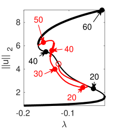
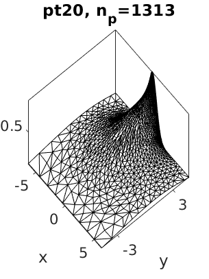
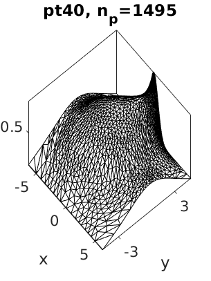
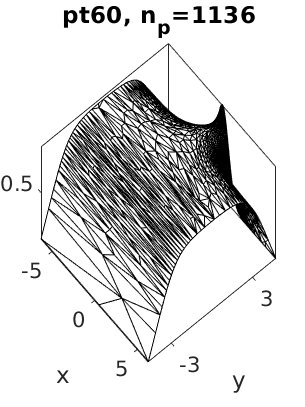
(b) Sample plots from red branch

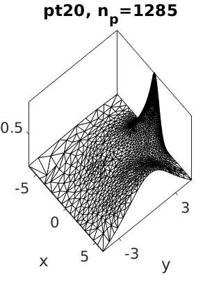
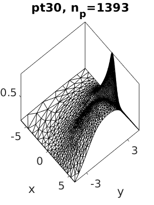
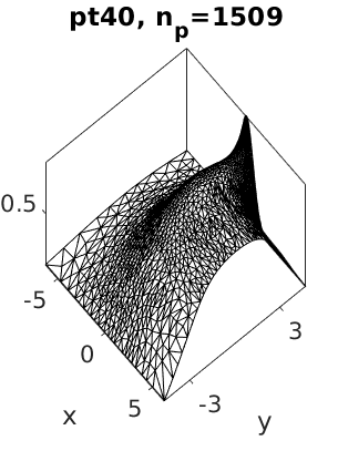
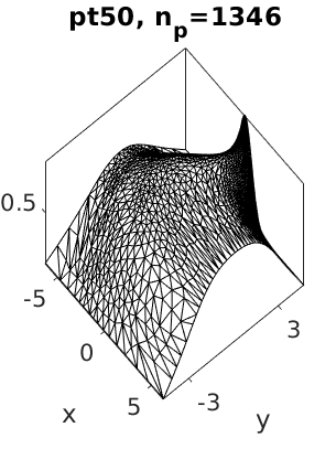
Figure 3: Example from cmds2. Continuing the primary solution branch in $\lambda$, fixed $\xi=0$ yields an ’imperfect bifurcation’ to the primary unimodal branch, and with an additional bifurcation to a branch with broken $x\mapsto-x$ symmetry, which, somewhat unexpectedly contains stable solutions, e.g., pt40.

3.2 3D

In ac3Dwspot we consider analogous BCs as in (10), i.e.

$$G(u):=-c\Delta u-\lambda u-u^{3}+\gamma u^{5}=0\text{ in $\Omega$},$$ (11a)

$$\left\{\begin{array}[]{l}\text{$u=\exp(-(x-\xi)^{2}-z^{2})$ on $\Gamma_{3}=\{y=-3\pi/2\}$, parameter $\xi$,}\\ \text{$u=0$ on $\Gamma_{5}=\{y=3\pi/2\}$, }\\ \text{${\partial}_{n}u=0$ on ${\partial}\Omega\setminus(\Gamma_{3}\cup\Gamma_{5})$.}\end{array}\right.$$ (11e)

For 3D cuboids as generated by stanpdeo3D, the order of the boundary faces is bottom, left, front, right, back, top, which leads to a straightforward modification of sGws from 2D to 3D. In cmds1 we again we start with a continuation in $\xi$ in the (here weakly) subcritical regime $\lambda=0$, with the main results given in Fig. 4, using a very coarse initial mesh with $n_{p}=3543$ to illustrate some effects and important settings for mesh–adaptation.

(a) coarse initial mesh	(b) refinement of (a)	(c) coarsening of (b)

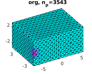
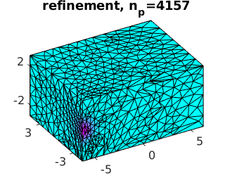
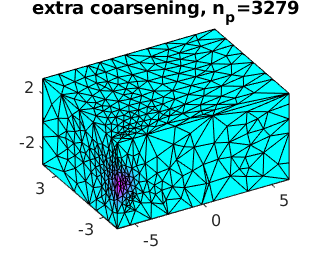
(d) BD, cont. with fixed (red) and adaptive (blue) meshes, and sample solutions from the blue branch

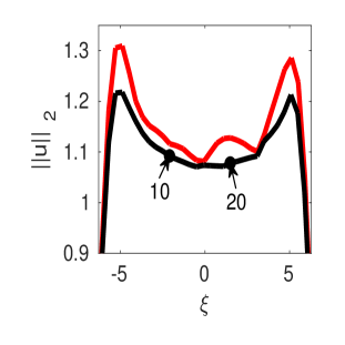
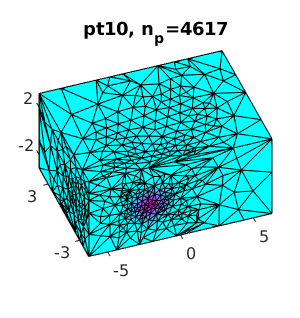
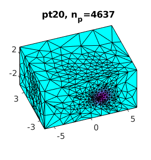
Figure 4: Selected plots from ac3Dwspot/cmds1. Colorscale in all plots from $u=0$ to $u=1$.

Solutions on this coarse mesh look quite reasonable, see (a), and adaptive refinement (b) and subsequent coarsening (with p.trcop.sw=5, see Table 2) yield solutions which are visually the same, at least in the surface plots. However, for continuation on the fixed original coarse mesh from (a), for instance the $L^{2}$–norm shows some unexpected fluctuations (red branch in (d)), e.g., for $\xi\in(0,2)$. These are essentially due to the spot at a given $\xi$ sitting on (close to) a mesh point, or in between two mesh points. The black branch in (d) is from continuation with mesh adaptation every 5th step, starting from the solution in (c), and setting p.trcop.npb=3000 to coarsen a given mesh to at most 3000 mesh points before refinement. The two sample plots on the right of (d) are from this blue branch. Some main observations are:

1. The $L^{2}$–norm on the adapted meshes is generally slightly smaller than on the (coarse) uniform mesh, and

2. The trullekrul coarsening (to less than 3000 mesh points) — refine approach yields nicely moving grids of small size with the finest meshing centered at the spots after each refinement.

3. Even though we only adapt every 5 steps, during which the spot moves to distance about 1 to 1.5 from the finest meshing, the black branch is reasonably smooth. However, if for instance we set amod=10 (such that the spot moves further away before remeshing), then visible jumps occur in the $L^{2}$–norm branch at each adaptation.

As in 2D, in cmds2 we then switch to $\lambda$ continuation, see Fig. 3.2. The basic behavior is as in 2D, i.e., the black branch turns into the primary unimodal (+spot) branch by an imperfect bifurcation, and there are now four bifurcation points connected by branches with broken $x\to-x$ symmetry.

hu,ho

sl

(a) BD and sample plots (lower left quarter domain) from the primary $\lambda$ branch

(b) Sample plots (lower half of domain) from the first bifurcating branch (red)

Listing 5: Selected plots from ac3Dwspot/cmds2. Colorscale in all solution plots from $u=0$ to $u=1$. Fixed $\xi=0$, continuation in $\lambda$, yielding imperfect bifurcation to primary unimodal branch (black). At the first BP, a solution with broken $y\mapsto-y$ symmetry bifurcates, at the third BP the $z\mapsto-z$ symmetry is broken. The inner interfaces between $u=0$ and $u=1$ suggest a larger $n_{p}$. Some options used are: amod=8; trop.qualP=2.25; trcop.npb=8000.

References

- [CSX07] Long Chen, Pengtao Sun, and Jinchao Xu. Optimal anisotropic meshes for minimizing interpolation errors in -norm. Math. Comp., 76(257):179–204, 2007.
- [dWDR+19] H. de Witt, T. Dohnal, J.D.M. Rademacher, H. Uecker, and D. Wetzel. pde2path - Quickstart guide and reference card, 2019.
- [Jen17] K.E. Jensen. A matlab script for solving 2d/3d miminum compliance problems using anisotropic mesh adaptation. 26th international meshing roundtable, 203:102–114, 2017.
- [JG16] K.E. Jensen and G. Gorman. Details of tetrahedral anisotropic mesh adaptation. Computer Physics Communications, 201:135–143, 2016.
- [LSB05] Xiangrong Li, M. S. Shephard, and M. W. Beall. 3D anisotropic mesh adaptation by mesh modification. Comput. Methods Appl. Mech. Engrg., 194(48-49):4915–4950, 2005.
- [RU19] J.D.M. Rademacher and H. Uecker. The OOPDE setting of pde2path – a tutorial via some Allen-Cahn models, 2019.
- [Uec19a] H. Uecker. Hopf bifurcation and time periodic orbits with pde2path – algorithms and applications. Comm. in Comp. Phys, 25(3):812–852, 2019.
- [Uec19b] H. Uecker. Pattern formation with pde2path – a tutorial, 2019.
- [Uec19c] H. Uecker. www.staff.uni-oldenburg.de/hannes.uecker/pde2path, 2019.
- [UWR14] H. Uecker, D. Wetzel, and J.D.M. Rademacher. pde2path – a Matlab package for continuation and bifurcation in 2D elliptic systems. NMTMA, 7:58–106, 2014.