Cosmology of fermionic dark energy coupled to curvature
Abstract
A formulation of cosmology driven by fermions is studied. Assumption that the expectation value of the fermion bilinear is non-zero simplifies the homogeneous solution of the Dirac equations and connects the spinor field with the scale parameter of the universe. With coupling between the Einstein term and spinor field , the possibility for a late time interaction emerges. In that way, the early universe agrees with CDM model, but for the late universe the new integrating term dominates.
I Introduction
The standard model of cosmology, the CDM model, requires a dark energy (DE) component responsible for the observed late-time acceleration of the expansion rate. The tension between the values of the Hubble constant obtained from the late universe measurements Riess et al. (2019, 2021) and those from the Cosmic Microwave Background (CMB) by Planck Collaboration Aghanim et al. (2020) is larger than . This tension is one of the biggest challenges in modern cosmology that indicates a possible new physics Di Valentino et al. (2021a, b, c); Efstathiou (2020); Borhanian et al. (2020); Hryczuk and Jodłowski (2020); Klypin et al. (2021); Ivanov et al. (2020); Chudaykin et al. (2020); Lyu et al. (2021); Alestas et al. (2020); Motloch and Hu (2020); Frusciante et al. (2020); Kumar (2021); Di Valentino et al. (2021d); Alestas et al. (2021); Benisty et al. (2021).
The search for constituents responsible for accelerated periods in the evolution of the universe is a big topic in cosmology. Several candidates has been tested for describing both the inflationary period and the present accelerated era: scalar fields, equations of state and cosmological constants. Fermionic fields has also been tested as gravitational sources of an expanding universe Samojeden et al. (2010) with cosmological applications Chimento et al. (2008); Myrzakulov (2010); Ribas et al. (2016). Fermions as dark matter are widely discussed such as neutrino dark matter, or supersymmetric extensions of the Standard Model Roszkowski (1993); Roulet (1993); Drees (1994); Jungman et al. (1996); Martin (1998); Bertone et al. (2005); Feng (2010); Ellis and Olive (2010). In some of these models the fermionic field plays the role of the inflaton in the early period of the universe and of dark energy for the late universe Benisty et al. (2019a).
As we will see, under the simplest assumption of an homogeneous expansion the Noether symmetry yields the relation where is the fermionic field, and is the scale factor of the universe. This relation impose a different scenario than the scalar fields in cosmology and gives another candidates for dark matter and dark energy Zee (1980); Cooper and Venturi (1981); Rossi et al. (2019); Ballardini et al. (2020); Ballesteros et al. (2020). In the inflationary scenario the scalar fields need to be slow roll, which mean that for e-folds the scalar field value should be around the same value Starobinsky (1979); Kazanas (1980); Starobinsky (1980); Guth (1981); Linde (1982); Albrecht and Steinhardt (1982); Barrow and Ottewill (1983); Blau et al. (1987); Barrow and Paliathanasis (2016, 2018); Olive (1990); Linde (1994); Liddle et al. (1994); Lidsey et al. (1997); Cervantes-Cota and Dehnen (1995); Berera (1995); Armendariz-Picon et al. (1999); Kanti and Olive (1999); Garriga and Mukhanov (1999); Gordon et al. (2000); Bassett et al. (2006); Chen and Wang (2010); Germani and Kehagias (2010); Kobayashi et al. (2010); Feng et al. (2010); Burrage et al. (2011); Kobayashi et al. (2011); Ohashi and Tsujikawa (2012); Hossain et al. (2014); Wali Hossain et al. (2015); Cai et al. (2015); Geng et al. (2015); Kamali et al. (2016); Geng et al. (2017); Benisty and Guendelman (2018); Dalianis et al. (2019); Dalianis and Tringas (2019); Benisty et al. (2020a); Benisty (2019); Benisty et al. (2020b, 2019b); Staicova and Stoilov (2019a); Staicova (2019); Staicova and Stoilov (2019b); Guendelman (1999); Guendelman et al. (2015); Qiu et al. (2020). However, the corresponding fermionic fields evolves times. Therefore, any similarity between scalar and fermions is only accidental.
The corresponding theory that involve fermions instead of scalars are the "Fermions Tensor Theories" (FTT). Here we show that a simple coupling to curvature gives an exaltation to tension. This new coupling is dominant for the late universe and gives closer value to local measurement of the Hubble constant from Riess et al. (2019). For the early universe we get the CDM model.
The plan of the work is as follows: Section II formulates the tetrad formalism for a homogeneous expansion. Section III suggests the FTT with the solved equations of motions. Section IV gives the extended theory we test. Section V test the extended model with the latest observations. Section VI summarizes the results that finalizes in VII.
II Fermions in Curved Spacetime
In this section we construct the scenario of fermionic cosmology in FTT. We first briefly review the basics of fermions in curved spacetime, and then we present the Lagrangian of the model, extracting the equations of motion. Fermions in a cosmological background have been widely discussed in Saha (2020). The tetrad formalism was used to combine the gauge group of general relativity with a spinor matter field. The tetrad and the metric tensors are related through
| (1) |
with Latin indices refer to the local inertial frame with the Minkowski metric , while Greek indices denote the local coordinate basis of the manifold.
are the Dirac matrices in the standard representation (flat spacetime). The Dirac matrices in curved space are obtained using the tetrads , labeled with a Latin index. The generalized Dirac matrices obey the Clifford algebra . The definition for the covariant derivative for spinors reads:
| (2) |
| (3) |
where is the spin connection, and is the Christoffel symbols:
| (4) |
We consider the Friedman Lemat̂re Robertson Walker (FLRW) homogeneous and isotropic metric:
| (5) |
with the scale factor and the Lapse function . Through (1) the tetrad components are found to be
| (6) |
Moreover, the covariant version of the Dirac matrices are
| (7) |
while the spin connection becomes
| (8) |
= da/dt, is the time derivative. This formulation is the basic mathematics for the Fermion tensor theories (FTT).
III Fermion Tensor Theories
In this section we apply the above fermionic formulation at a cosmological framework, focusing on late-time universe. The framework of FTT has a similar form to Scalar Tensor Theories and discussed in details in Saha (2020); de Souza and Kremer (2008). The FTT read:
| (9) |
where is the Ricci scalar, and are the spinor field and its adjoint, respectively. We set . The scalar multiples the fermionic field and its conjugate field. is the function that couples the Einstein term and the self-interaction potential density of the fermionic field. The kinetic term of the spinors is the same as the kinetic term from Dirac equation. However, FTT suggest a generic coupling function .
For and the FTT reduce to the Dirac equation in curved spacetime. For the metric (5) the action (9) reduces to the form:
| (10) |
is the time derivative. The solution is obtained via the complete set of variations: the scale factor and the spinor field . The variation with respect to field (extended Dirac equation) yields:
| (11) |
and similarly for :
| (12) |
is the Hubble function: . By multiplying the first equation by from the left hand side and the second equation by from the right hand, the equations get the same form. The sum of those two equations gives:
| (13) |
with the solution:
| (14) |
is a dimensionless integration constant that emerges from Eq (14). The quantity is thus the total gas energy density. The variation w.r.t the Lapse function yields the Friedmann’s equation:
| (15) |
with the gauge . Together with the set of Eq. (14) one can find the whole evolution of the model.
IV Decaying curvature coupling
The CDM model emerges from the simplest expression for the potential. A simple example is a linear expansion for both functions:
| (16) |
with the dimensions: The corresponding Hubble function reads:
| (17) |
with the dark matter component
| (18) |
without other fields. is the predicted value of at present time. In this model the matter component comes from the fermions field. de Souza and Kremer (2008) uses the Noether symmetry in order to find the coupling function . The paper suggests or . The case of gives a divergent solution. Inspired by de Souza and Kremer (2008) solutions, we choose the following combinations, with a power-law extension:
| (19) |
The corresponding Hubble function yields:
| (20) |
with: . The parameter is combined from the parameters , and . the parameter is a dimensionless parameter. Because of the ambiguity with the other parameters we use the parameter instead. The new parameterization changes the behavior of the late universe, since for large redshifts the term decays. Hence the term "Decaying coupled Fermions to curvature". For the future expansion the model predicts different behavior.
V Observational Constraints
In the following we describe the observational data sets along with the relevant statistics in constraining the model.
V.0.1 Direct measurements of the Hubble expansion
Cosmic Chronometers (CC): The data set exploits the evolution of differential ages of passive galaxies at different redshifts to directly constrain the Hubble parameter Jimenez and Loeb (2002). We use uncorrelated 30 CC measurements of discussed in Moresco et al. (2012a, b); Moresco (2015); Moresco et al. (2016). Here, the corresponding function reads:
| (21) |
where is the observed Hubble rates at redshift () and is the predicted one from the model.
| Parameter | free | CDM | ||
|---|---|---|---|---|
V.0.2 Standard Candles
As Standard Candles (SC) we use measurements of the Pantheon Type Ia supernova Scolnic et al. (2018). The model parameters of the models are to be fitted with, comparing the observed value to the theoretical value of the distance moduli which are the logarithms:
| (22) |
where and are the apparent and absolute magnitudes and is the nuisance parameter that has been marginalized. The luminosity distance is defined by,
| (23) |
Here corresponds to spatially flat spacetime. Following the approach used in (Di Pietro and Claeskens (2003); Nesseris and Perivolaropoulos (2004); Perivolaropoulos (2005); Lazkoz et al. (2005)), we assumed no prior constraint on , which is just some constant, and we integrated the probabilities over . The integrated yields:
| (24) |
where:
| (25a) | |||
| (25b) | |||
| (25c) |
Here is the observed luminosity, is its error, and the is the luminosity distance. The values of and don’t change the marginalized . In order to use the covariance matrix provided for the Pantheon dataset, one needs to transform as follows:
| (26a) | |||
| (26b) | |||
| (26c) |
where , is the unit matrix, and is the inverse covariance matrix of the dataset.
V.0.3 Joint analysis and model selection
In order to perform a joint statistical analysis of cosmological probes we need to use the total likelihood function, consequently the expression is given by:
| (27) |
Regarding the problem of likelihood maximization, we use an affine-invariant Markov Chain Monte Carlo sampler Foreman-Mackey et al. (2013), as it is implemented within the open-source packaged Polychord Handley et al. (2015) with the GetDist packages Lewis (2019) to present the results. The prior we choose is with a uniform distribution, where , and , for the additional parameters.
VI Results
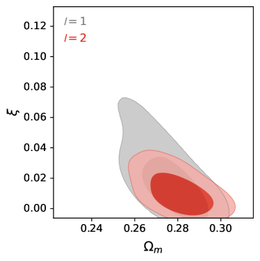
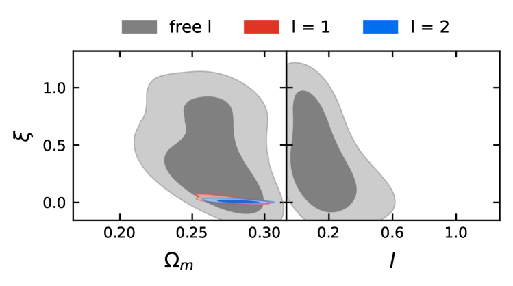
The table under 2 summarizes the best fit results for different models. Fig 1,2 shows the posterior distribution for the vs. and . For the cases the is assumed to be a constant, i.e. or , the part slightly changes from for the CDM model: For the matter part gives and for the matter part yields . For the dynamical the matter part still gives . From this comparison we can see the model requires a bit smaller values for the matter part, and does not sensitive to the value of so much. The conclusion is similar: the model requires a bit smaller values for the dark energy part, and does not sensitive to the value of by much.
The additional parameters gets different constraints from different models: For the parameter is constrained to be , and for the parameter is . For the dynamical case, the additional parameter is , with . For these cases it possible to see that CDM is part from the posterior distribution. For the general case, if we approach to the early universe which referrers to larger , the modified model is changes to CDM model, since the new term becomes negligible.
VII Discussion
In this work, we have studied in detail the phenomenology of a simple generalized fermionic field model for dark energy and dark matter. Assumption that the expectation value of the fermion bilinear is non-zero (which is the case in the presence of dark matter) simplifies the homogeneous solution of the Dirac equations and connects the spinor field with the scale parameter of the universe. With coupling between the Einstein term and spinor field, the possibility for a late time interaction emerges. In that way, the early universe agrees with CDM model, but for the late universe the new interacting term dominates.
In this model we treat the fermions as the source to the dark matter part. Some plausible option that fits to this model the neutrino dark matter in supersymmetric extensions of the Standard Model. In addition to the matter part, we coupled the fermionic field to the Einstein part using function. Extending the Noether Symmetry that imposes some we set a general form of the function. The form for high redshifts decays, but for small redshifts the model changes from the CDM.
We test a combine data set of the Cosmic Chronometers and Standard Candles of the Type Ia Supernova. The decaying coupling reveals the capabilities of the scenario and makes it a good candidate for the description of nature. In the future it would be interesting to extended the current work for the perturbation level and to test whenever this kind of coupling may explain the tension while on the homogenous level can keep CDM for the early Universe. This work should be done with the full analysis of the perturbation solution of the fermionic field.
Acknowledgements.
I would like to thank Alexander Kaganovich, Emil Nissimov & Sventlana Pacheva for helpful comments and advice. This article is supported by COST Action CA15117 "Cosmology and Astrophysics Network for Theoretical Advances and Training Action" (CANTATA) of the COST (European Cooperation in Science and Technology) and the Actions CA16104 and CA18108. Finally I would like to thank to the Grants Committee of the Rothschild and the Blavatnik Cambridge Fellowships for generous supports.References
- Riess et al. (2019) A. G. Riess, S. Casertano, W. Yuan, L. M. Macri, and D. Scolnic, Astrophys. J. 876, 85 (2019), arXiv:1903.07603 [astro-ph.CO] .
- Riess et al. (2021) A. G. Riess, S. Casertano, W. Yuan, J. B. Bowers, L. Macri, J. C. Zinn, and D. Scolnic, Astrophys. J. Lett. 908, L6 (2021), arXiv:2012.08534 [astro-ph.CO] .
- Aghanim et al. (2020) N. Aghanim et al. (Planck), Astron. Astrophys. 641, A6 (2020), [Erratum: Astron.Astrophys. 652, C4 (2021)], arXiv:1807.06209 [astro-ph.CO] .
- Di Valentino et al. (2021a) E. Di Valentino et al., Astropart. Phys. 131, 102606 (2021a), arXiv:2008.11283 [astro-ph.CO] .
- Di Valentino et al. (2021b) E. Di Valentino et al., Astropart. Phys. 131, 102605 (2021b), arXiv:2008.11284 [astro-ph.CO] .
- Di Valentino et al. (2021c) E. Di Valentino et al., Astropart. Phys. 131, 102604 (2021c), arXiv:2008.11285 [astro-ph.CO] .
- Efstathiou (2020) G. Efstathiou, (2020), arXiv:2007.10716 [astro-ph.CO] .
- Borhanian et al. (2020) S. Borhanian, A. Dhani, A. Gupta, K. G. Arun, and B. S. Sathyaprakash, Astrophys. J. Lett. 905, L28 (2020), arXiv:2007.02883 [astro-ph.CO] .
- Hryczuk and Jodłowski (2020) A. Hryczuk and K. Jodłowski, Phys. Rev. D 102, 043024 (2020), arXiv:2006.16139 [hep-ph] .
- Klypin et al. (2021) A. Klypin, V. Poulin, F. Prada, J. Primack, M. Kamionkowski, V. Avila-Reese, A. Rodriguez-Puebla, P. Behroozi, D. Hellinger, and T. L. Smith, Mon. Not. Roy. Astron. Soc. 504, 769 (2021), arXiv:2006.14910 [astro-ph.CO] .
- Ivanov et al. (2020) M. M. Ivanov, Y. Ali-Haïmoud, and J. Lesgourgues, Phys. Rev. D 102, 063515 (2020), arXiv:2005.10656 [astro-ph.CO] .
- Chudaykin et al. (2020) A. Chudaykin, D. Gorbunov, and N. Nedelko, JCAP 08, 013 (2020), arXiv:2004.13046 [astro-ph.CO] .
- Lyu et al. (2021) K.-F. Lyu, E. Stamou, and L.-T. Wang, Phys. Rev. D 103, 015004 (2021), arXiv:2004.10868 [hep-ph] .
- Alestas et al. (2020) G. Alestas, L. Kazantzidis, and L. Perivolaropoulos, Phys. Rev. D 101, 123516 (2020), arXiv:2004.08363 [astro-ph.CO] .
- Motloch and Hu (2020) P. Motloch and W. Hu, Phys. Rev. D 101, 083515 (2020), arXiv:1912.06601 [astro-ph.CO] .
- Frusciante et al. (2020) N. Frusciante, S. Peirone, L. Atayde, and A. De Felice, Phys. Rev. D 101, 064001 (2020), arXiv:1912.07586 [astro-ph.CO] .
- Kumar (2021) S. Kumar, Phys. Dark Univ. 33, 100862 (2021), arXiv:2102.12902 [astro-ph.CO] .
- Di Valentino et al. (2021d) E. Di Valentino, O. Mena, S. Pan, L. Visinelli, W. Yang, A. Melchiorri, D. F. Mota, A. G. Riess, and J. Silk, Class. Quant. Grav. 38, 153001 (2021d), arXiv:2103.01183 [astro-ph.CO] .
- Alestas et al. (2021) G. Alestas, L. Kazantzidis, and L. Perivolaropoulos, Phys. Rev. D 103, 083517 (2021), arXiv:2012.13932 [astro-ph.CO] .
- Benisty et al. (2021) D. Benisty, D. Vasak, J. Kirsch, and J. Struckmeier, Eur. Phys. J. C 81, 125 (2021), arXiv:2101.07566 [gr-qc] .
- Samojeden et al. (2010) L. L. Samojeden, F. P. Devecchi, and G. M. Kremer, Phys. Rev. D 81, 027301 (2010), arXiv:1001.2285 [gr-qc] .
- Chimento et al. (2008) L. P. Chimento, F. P. Devecchi, M. I. Forte, and G. M. Kremer, Class. Quant. Grav. 25, 085007 (2008), arXiv:0707.4455 [gr-qc] .
- Myrzakulov (2010) R. Myrzakulov, (2010), arXiv:1011.4337 [astro-ph.CO] .
- Ribas et al. (2016) M. O. Ribas, F. P. Devecchi, and G. M. Kremer, Mod. Phys. Lett. A 31, 1650039 (2016), arXiv:1602.06874 [gr-qc] .
- Roszkowski (1993) L. Roszkowski, in INFN Eloisatron Project: 23rd Workshop: The Decay Properties of SUSY Particles (1993) arXiv:hep-ph/9302259 .
- Roulet (1993) E. Roulet, in 28th Rencontres de Moriond: Electroweak Interactions and Unified Theories (1993) pp. 391–396.
- Drees (1994) M. Drees, in International Conference on Non-Accelerator Particle Physics - ICNAPP (1994) pp. 0261–271, arXiv:hep-ph/9402211 .
- Jungman et al. (1996) G. Jungman, M. Kamionkowski, and K. Griest, Phys. Rept. 267, 195 (1996), arXiv:hep-ph/9506380 .
- Martin (1998) S. P. Martin, Adv. Ser. Direct. High Energy Phys. 18, 1 (1998), arXiv:hep-ph/9709356 .
- Bertone et al. (2005) G. Bertone, D. Hooper, and J. Silk, Phys. Rept. 405, 279 (2005), arXiv:hep-ph/0404175 .
- Feng (2010) J. L. Feng, Ann. Rev. Astron. Astrophys. 48, 495 (2010), arXiv:1003.0904 [astro-ph.CO] .
- Ellis and Olive (2010) J. Ellis and K. A. Olive, , 142 (2010), arXiv:1001.3651 [astro-ph.CO] .
- Benisty et al. (2019a) D. Benisty, E. I. Guendelman, E. N. Saridakis, H. Stoecker, J. Struckmeier, and D. Vasak, Phys. Rev. D 100, 043523 (2019a), arXiv:1905.03731 [gr-qc] .
- Zee (1980) A. Zee, Phys. Rev. Lett. 44, 703 (1980).
- Cooper and Venturi (1981) F. Cooper and G. Venturi, Phys. Rev. D 24, 3338 (1981).
- Rossi et al. (2019) M. Rossi, M. Ballardini, M. Braglia, F. Finelli, D. Paoletti, A. A. Starobinsky, and C. Umiltà, Phys. Rev. D 100, 103524 (2019), arXiv:1906.10218 [astro-ph.CO] .
- Ballardini et al. (2020) M. Ballardini, M. Braglia, F. Finelli, D. Paoletti, A. A. Starobinsky, and C. Umiltà, JCAP 10, 044 (2020), arXiv:2004.14349 [astro-ph.CO] .
- Ballesteros et al. (2020) G. Ballesteros, A. Notari, and F. Rompineve, JCAP 11, 024 (2020), arXiv:2004.05049 [astro-ph.CO] .
- Starobinsky (1979) A. A. Starobinsky, JETP Lett. 30, 682 (1979).
- Kazanas (1980) D. Kazanas, Astrophys. J. Lett. 241, L59 (1980).
- Starobinsky (1980) A. A. Starobinsky, Phys. Lett. B 91, 99 (1980).
- Guth (1981) A. H. Guth, Phys. Rev. D 23, 347 (1981).
- Linde (1982) A. D. Linde, Phys. Lett. B 108, 389 (1982).
- Albrecht and Steinhardt (1982) A. Albrecht and P. J. Steinhardt, Phys. Rev. Lett. 48, 1220 (1982).
- Barrow and Ottewill (1983) J. D. Barrow and A. C. Ottewill, J. Phys. A 16, 2757 (1983).
- Blau et al. (1987) S. K. Blau, E. I. Guendelman, and A. H. Guth, Phys. Rev. D 35, 1747 (1987).
- Barrow and Paliathanasis (2016) J. D. Barrow and A. Paliathanasis, Phys. Rev. D 94, 083518 (2016), arXiv:1609.01126 [gr-qc] .
- Barrow and Paliathanasis (2018) J. D. Barrow and A. Paliathanasis, Gen. Rel. Grav. 50, 82 (2018), arXiv:1611.06680 [gr-qc] .
- Olive (1990) K. A. Olive, Phys. Rept. 190, 307 (1990).
- Linde (1994) A. D. Linde, Phys. Rev. D 49, 748 (1994), arXiv:astro-ph/9307002 .
- Liddle et al. (1994) A. R. Liddle, P. Parsons, and J. D. Barrow, Phys. Rev. D 50, 7222 (1994), arXiv:astro-ph/9408015 .
- Lidsey et al. (1997) J. E. Lidsey, A. R. Liddle, E. W. Kolb, E. J. Copeland, T. Barreiro, and M. Abney, Rev. Mod. Phys. 69, 373 (1997), arXiv:astro-ph/9508078 .
- Cervantes-Cota and Dehnen (1995) J. L. Cervantes-Cota and H. Dehnen, Nucl. Phys. B 442, 391 (1995), arXiv:astro-ph/9505069 .
- Berera (1995) A. Berera, Phys. Rev. Lett. 75, 3218 (1995), arXiv:astro-ph/9509049 .
- Armendariz-Picon et al. (1999) C. Armendariz-Picon, T. Damour, and V. F. Mukhanov, Phys. Lett. B 458, 209 (1999), arXiv:hep-th/9904075 .
- Kanti and Olive (1999) P. Kanti and K. A. Olive, Phys. Lett. B 464, 192 (1999), arXiv:hep-ph/9906331 .
- Garriga and Mukhanov (1999) J. Garriga and V. F. Mukhanov, Phys. Lett. B 458, 219 (1999), arXiv:hep-th/9904176 .
- Gordon et al. (2000) C. Gordon, D. Wands, B. A. Bassett, and R. Maartens, Phys. Rev. D 63, 023506 (2000), arXiv:astro-ph/0009131 .
- Bassett et al. (2006) B. A. Bassett, S. Tsujikawa, and D. Wands, Rev. Mod. Phys. 78, 537 (2006), arXiv:astro-ph/0507632 .
- Chen and Wang (2010) X. Chen and Y. Wang, JCAP 04, 027 (2010), arXiv:0911.3380 [hep-th] .
- Germani and Kehagias (2010) C. Germani and A. Kehagias, Phys. Rev. Lett. 105, 011302 (2010), arXiv:1003.2635 [hep-ph] .
- Kobayashi et al. (2010) T. Kobayashi, M. Yamaguchi, and J. Yokoyama, Phys. Rev. Lett. 105, 231302 (2010), arXiv:1008.0603 [hep-th] .
- Feng et al. (2010) C.-J. Feng, X.-Z. Li, and E. N. Saridakis, Phys. Rev. D 82, 023526 (2010), arXiv:1004.1874 [astro-ph.CO] .
- Burrage et al. (2011) C. Burrage, C. de Rham, D. Seery, and A. J. Tolley, JCAP 01, 014 (2011), arXiv:1009.2497 [hep-th] .
- Kobayashi et al. (2011) T. Kobayashi, M. Yamaguchi, and J. Yokoyama, Prog. Theor. Phys. 126, 511 (2011), arXiv:1105.5723 [hep-th] .
- Ohashi and Tsujikawa (2012) J. Ohashi and S. Tsujikawa, JCAP 10, 035 (2012), arXiv:1207.4879 [gr-qc] .
- Hossain et al. (2014) M. W. Hossain, R. Myrzakulov, M. Sami, and E. N. Saridakis, Phys. Rev. D 90, 023512 (2014), arXiv:1402.6661 [gr-qc] .
- Wali Hossain et al. (2015) M. Wali Hossain, R. Myrzakulov, M. Sami, and E. N. Saridakis, Int. J. Mod. Phys. D 24, 1530014 (2015), arXiv:1410.6100 [gr-qc] .
- Cai et al. (2015) Y.-F. Cai, J.-O. Gong, S. Pi, E. N. Saridakis, and S.-Y. Wu, Nucl. Phys. B 900, 517 (2015), arXiv:1412.7241 [hep-th] .
- Geng et al. (2015) C.-Q. Geng, M. W. Hossain, R. Myrzakulov, M. Sami, and E. N. Saridakis, Phys. Rev. D 92, 023522 (2015), arXiv:1502.03597 [gr-qc] .
- Kamali et al. (2016) V. Kamali, S. Basilakos, and A. Mehrabi, Eur. Phys. J. C 76, 525 (2016), arXiv:1604.05434 [gr-qc] .
- Geng et al. (2017) C.-Q. Geng, C.-C. Lee, M. Sami, E. N. Saridakis, and A. A. Starobinsky, JCAP 06, 011 (2017), arXiv:1705.01329 [gr-qc] .
- Benisty and Guendelman (2018) D. Benisty and E. I. Guendelman, Int. J. Mod. Phys. A 33, 1850119 (2018), arXiv:1710.10588 [gr-qc] .
- Dalianis et al. (2019) I. Dalianis, A. Kehagias, and G. Tringas, JCAP 01, 037 (2019), arXiv:1805.09483 [astro-ph.CO] .
- Dalianis and Tringas (2019) I. Dalianis and G. Tringas, Phys. Rev. D 100, 083512 (2019), arXiv:1905.01741 [astro-ph.CO] .
- Benisty et al. (2020a) D. Benisty, E. I. Guendelman, E. Nissimov, and S. Pacheva, Symmetry 12, 734 (2020a), arXiv:2003.04723 [gr-qc] .
- Benisty (2019) D. Benisty, (2019), arXiv:1912.11124 [gr-qc] .
- Benisty et al. (2020b) D. Benisty, E. I. Guendelman, E. Nissimov, and S. Pacheva, Nucl. Phys. B 951, 114907 (2020b), arXiv:1907.07625 [astro-ph.CO] .
- Benisty et al. (2019b) D. Benisty, E. Guendelman, E. Nissimov, and S. Pacheva, Eur. Phys. J. C 79, 806 (2019b), arXiv:1906.06691 [gr-qc] .
- Staicova and Stoilov (2019a) D. Staicova and M. Stoilov, Int. J. Mod. Phys. A 34, 1950099 (2019a), arXiv:1906.08516 [gr-qc] .
- Staicova (2019) D. Staicova, AIP Conf. Proc. 2075, 100003 (2019), arXiv:1808.08890 [gr-qc] .
- Staicova and Stoilov (2019b) D. Staicova and M. Stoilov, Symmetry 11, 1387 (2019b), arXiv:1806.08199 [gr-qc] .
- Guendelman (1999) E. I. Guendelman, Mod. Phys. Lett. A 14, 1397 (1999), arXiv:hep-th/0106084 .
- Guendelman et al. (2015) E. Guendelman, R. Herrera, P. Labrana, E. Nissimov, and S. Pacheva, Gen. Rel. Grav. 47, 10 (2015), arXiv:1408.5344 [gr-qc] .
- Qiu et al. (2020) T. Qiu, T. Katsuragawa, and S. Ni, Eur. Phys. J. C 80, 1163 (2020), arXiv:2003.12755 [astro-ph.CO] .
- Saha (2020) B. Saha, Astrophys. Space Sci. 365, 68 (2020), arXiv:1908.05109 [gr-qc] .
- de Souza and Kremer (2008) R. C. de Souza and G. M. Kremer, Class. Quant. Grav. 25, 225006 (2008), arXiv:0807.1965 [gr-qc] .
- Jimenez and Loeb (2002) R. Jimenez and A. Loeb, Astrophys. J. 573, 37 (2002), arXiv:astro-ph/0106145 .
- Moresco et al. (2012a) M. Moresco, L. Verde, L. Pozzetti, R. Jimenez, and A. Cimatti, JCAP 07, 053 (2012a), arXiv:1201.6658 [astro-ph.CO] .
- Moresco et al. (2012b) M. Moresco et al., JCAP 08, 006 (2012b), arXiv:1201.3609 [astro-ph.CO] .
- Moresco (2015) M. Moresco, Mon. Not. Roy. Astron. Soc. 450, L16 (2015), arXiv:1503.01116 [astro-ph.CO] .
- Moresco et al. (2016) M. Moresco, L. Pozzetti, A. Cimatti, R. Jimenez, C. Maraston, L. Verde, D. Thomas, A. Citro, R. Tojeiro, and D. Wilkinson, JCAP 05, 014 (2016), arXiv:1601.01701 [astro-ph.CO] .
- Scolnic et al. (2018) D. M. Scolnic et al., Astrophys. J. 859, 101 (2018), arXiv:1710.00845 [astro-ph.CO] .
- Di Pietro and Claeskens (2003) E. Di Pietro and J.-F. Claeskens, Mon. Not. Roy. Astron. Soc. 341, 1299 (2003), arXiv:astro-ph/0207332 .
- Nesseris and Perivolaropoulos (2004) S. Nesseris and L. Perivolaropoulos, Phys. Rev. D 70, 043531 (2004), arXiv:astro-ph/0401556 .
- Perivolaropoulos (2005) L. Perivolaropoulos, Phys. Rev. D 71, 063503 (2005), arXiv:astro-ph/0412308 .
- Lazkoz et al. (2005) R. Lazkoz, S. Nesseris, and L. Perivolaropoulos, JCAP 11, 010 (2005), arXiv:astro-ph/0503230 .
- Foreman-Mackey et al. (2013) D. Foreman-Mackey, D. W. Hogg, D. Lang, and J. Goodman, Publ. Astron. Soc. Pac. 125, 306 (2013), arXiv:1202.3665 [astro-ph.IM] .
- Handley et al. (2015) W. J. Handley, M. P. Hobson, and A. N. Lasenby, Mon. Not. Roy. Astron. Soc. 450, L61 (2015), arXiv:1502.01856 [astro-ph.CO] .
- Lewis (2019) A. Lewis, (2019), arXiv:1910.13970 [astro-ph.IM] .