Multi-level Convolutional Autoencoder Networks for Parametric Prediction of Spatio-temporal Dynamics

Abstract

A data-driven framework is proposed towards the end of predictive modeling of complex spatio-temporal dynamics, leveraging nested non-linear manifolds. Three levels of neural networks are used, with the goal of predicting the future state of a system of interest in a parametric setting. A convolutional autoencoder is used as the top level to encode the high dimensional input data along spatial dimensions into a sequence of latent variables. A temporal convolutional autoencoder (TCAE) serves as the second level, which further encodes the output sequence from the first level along the temporal dimension, and outputs a set of latent variables that encapsulate the spatio-temporal evolution of the dynamics. The use of dilated temporal convolutions grows the receptive field exponentially with network depth, allowing for efficient processing of long temporal sequences typical of scientific computations. A fully-connected network is used as the third level to learn the mapping between these latent variables and the global parameters from training data, and predict them for new parameters. For future state predictions, the second level uses a temporal convolutional network to predict subsequent steps of the output sequence from the top level. Latent variables at the bottom-most level are decoded to obtain the dynamics in physical space at new global parameters and/or at a future time. Predictive capabilities are evaluated on a range of problems involving discontinuities, wave propagation, strong transients, and coherent structures. The sensitivity of the results to different modeling choices is assessed. The results suggest that given adequate data and careful training, effective data-driven predictive models can be constructed. Perspectives are provided on the present approach and its place in the landscape of model reduction.

1 Introduction

Efficient and accurate prediction of complex spatio-temporal processes remains a problem of significant scientific and industrial value. Numerically well-resolved solutions of partial differential equations offer considerable insight into underlying physical processes, but continue to be prohibitively expensive in many query scenarios such as design, optimization and uncertainty quantification. As a consequence, reduced order and surrogate modeling approaches have emerged as a important avenue for research. In these approaches, an off-line stage aims to extract problem-specific low-dimensional information (such as a projection basis or a latent space) such that relatively inexpensive computations can be performed during the on-line predictive stage.

In projection-based Reduced Order Models (ROMs) [1], the most popular method to construct a low-dimensional linear subspace is the truncated proper orthogonal decomposition (POD) [2, 3], typically applied to a collection of solution snapshots. The governing equations of the full order model are then projected on to the lower dimensional subspace by choosing an appropriate test basis. Other linear basis construction methods include balanced truncation [4, 5], reduced basis methods [6, 7, 8], rational interpolation [9], and proper generalized decomposition [10, 11]. Linear basis ROMs have achieved considerable success in complex problems such as turbulent flows [12, 13, 14] and combustion instabilities [15, 16]. However, despite the choice of optimal test spaces afforded by Petrov–Galerkin methods [17], and closure modeling [18, 19, 20, 21], the linear trial space becomes ineffective in advection-dominated problems and many multiscale problems in general. While the associated challenges can be addressed to a certain degree by using adaptive basis [22, 23, 24], some of the fundamental challenges persist.

To overcome some of the limitations of the choice of a linear trial space, researchers have pursued the extraction of nonlinear trial manifolds. In Ref. [25], neural network-based compression in the form of an autoencoder [26] instead of POD in the development of a ROM for dynamical systems. Similar approaches have been applied to a range of fluid dynamic problems, including flow over airfoil [27], reacting flow [28], and improvement in accuracy has been reported, when compared to the use of linear bases. It should also be noted that POD methods do not provide basis functions that are compact spatially and/or temporally, and as a consequence, non-ideal for convection and transport-dominated problems. Neural networks with convolutional layers are capable of representing local features, offering promise in more efficiently representing multi-scale dynamics and convection-dominated problems. Indeed, the advantages of using nonlinear and local manifolds have been demonstrated [29, 30, 31].

Independent of the type of basis that is employed, ROM approaches can be broadly categorized into intrusive and non-intrusive methods. In intrusive ROMs, the full order governing equations are projected onto the reduced dimensional manifold using Galerkin [3, 32] and Petrov Galerkin [13, 20] formulations. To achieve computational efficiency in intrusive ROMs of complex non-linear PDEs, additional approximations are required. Sampling approaches such as missing point estimation (MPE) [33, 34], and empirical interpolation methods [35, 36, 37] have been developed to to restricting the computation of nonlinear terms to a subset of the state variables. Such methods introduce additional complexity and require careful treatment such as adaptive sampling and basis [22, 23] and oversampling [38]. It has to be mentioned that effective sampling approaches have not been developed for non-linear manifolds.

As an alternate to intrusive ROMs, latent data structures have been exploited to directly infer ROM equations from data. In Ref. [39], sparse system identification is performed based on a pre-collected dictionary of nonlinear equations. In Ref. [40], the idea of reducing arbitrary nonlinearity to quadratic-bilinearity via lifting is introduced, and applied to reacting flows in Refs. [41, 42]. Techniques for automated refinement and inference have also been proposed [43, 44].

Non-intrusive methods bypass the governing equations and process full order model solutions to develop data-driven surrogate models. Such methods rely on interpolation [45] or regression [46] operations. In this vein, neural networks have been applied to problems with arbitrary non-linearity [47, 48]. With recent advances in time-series processing techniques, the future state of reduced order variables [49] and the full field [50] have also been directly predicted. Time-series prediction has been popularly addressed using recurrent neural networks (RNN) [51] or long-short term memory networks (LSTM) [52]. In Ref. [53], state variables are compressed using an autoencoder and the resulting dynamics learned and predicted using a RNN. A similar approach is taken in Ref. [49], with a LSTM network replacing the RNN. Besides direct prediction of state variables, such techniques have also been applied in ROM closures [54].

In this work, we leverage neural networks for compression, convolution and regression towards the end of non-intrusive model reduction. An autoencoder [26] consists of an encoder part that compresses the high dimensional input into low dimensional latent variables, and a decoder part that reconstructs the original high dimensional input from the encoded latent variables. The encoder and decoder are trained jointly, yet can be used separately. By using nonlinear layers in an autoencoder, nonlinear model reduction can be performed. Convolutional neural networks (CNN) have been widely applied to image processing and achieved remarkable success. In the context of scientific computing, the localized nature of the kernel-based convolutional operations enables CNNs to identify and process coherent dynamics in arbitrary parts of the computational domain, which is difficult to achieve using global bases. Convolutional autoencoders have been demonstrated an effective approach for spatial field data compression [25, 29, 28, 31]. It should be mentioned that there are also convolutional models that are able to process spatial and temporal dimensions simultaneously, such as the ConvLSTM [55] and the spatio-temporal convolution [56], and have been successfully applied to popular deep learning tasks such as natural language processing and video generation. However, complex spatio-temporal systems in scientific computing often exhibit a much larger data size per frame, therefore such models cannot be easily applied.

For time series modeling tasks, the family of recurrent networks, e.g. the basic RNN [57], LSTM [58], GRU [59], are currently the most popular choice. Such networks process the time series data in a sequential manner, and recurrently updates a vector of hidden states at every input step of the time series data. Tremendous successes have been achieved with recurrent networks, applications including natural language processing [60, 61], time series forecasting [62, 63], automatic music composition [64], etc. Recently, temporal convolutional networks (TCN) [65] has been proposed for time series modeling. The TCN uses causal convolutions, which only operates on data before the current element, to process data in the temporal order. To handle long sequences, dilated convolution is used such that the receptive field grows exponentially with the depth of the network. This feature is especially helpful in practical engineering computations, which may require processing and predictions of thousands of frames. In Ref. [66], a comprehensive evaluation is conducted across a diverse range of sequence modeling tasks, and TCNs are shown to perform favorably compared to recurrent networks and also demonstrate a longer effective memory length, despite the theoretical advantage of unlimited memory for recurrent models. Other advantages of the TCN demonstrated in Ref. [66] include parallelism, stable gradients and low memory requirement in training. TCNs have proved to be a promising alternative in multiple canonical applications for recurrent models [67, 68, 69]. However, to our knowledge, TCNs have not been exploited in scientific computing applications.

We propose a framework that uses multiple levels of neural networks, namely spatial and temporal convolutional neural networks, autoencoders and multi-layer perceptrons to predict spatio-temporal dynamics in a parametric setting. The rest of this paper is organized as follows: An overview of the framework is provided in Sec. 2. Detailed neural network architectures and related neural network techniques are introduced in Sec. 3. Numerical tests are presented in Sec. 4. Perspectives on the present approach, and its place in the larger landscape of model reduction is presented in Sec. 5. A summary is given in Sec. 6. Sensitivity to various modeling choices is further explored in the appendices.

2 Goals and Framework Overview

We assume that the spatio-temporal process is represented by successive time snapshots of spatial field variables on a fixed uniform Cartesian grid. Further, the snapshots are evenly spaced in time. In each frame, the spatial field is characterized by several variables of interest, e.g. pressure, density, velocity components, etc. The variables at time index $i$ and their depedendence on parameters $\mu\in\mathds{R}^{\mu}$ is denoted by $\mathbf{q}(i;\mu)\in\mathds{R}^{n}$, where $n=(\prod_{j}n_{j})n_{var}$ is the total degrees of freedom per time step, $n_{j}$ is the number of grid points in direction $j\in{1,2,3}$, and $n_{var}$ is the number of variables. The sequence for a given parameter $\mu$ is denoted by $\mathbf{Q}(\mu)=[\mathbf{q}(1;\mu),\dots,\mathbf{q}(n_{t};{\mu})]\in\mathds{R}^{n\times n_{t}}$, where $n_{t}$ is the total number of time steps in the sequence.

The proposed framework targets three types of tasks, namely 1) prediction at new global parameters, 2) prediction for future time steps, and 3) a combination of the above. In the first task, sequences at several known parameters in a certain time period are provided as training data, and the time series at an unseen parameter in the same time period is predicted. The required input for this type of task is a new parameter $\mu^{*}$, and the target output is the corresponding sequence $\mathbf{Q}(\mu^{*})$. In the task of prediction for future time steps, the framework incrementally predicts one step in the future. By performing such predictions iteratively, multiple subsequent steps can be obtained. The required input is a sequence $\mathbf{Q}(\mu)$, and the target output is $\{\mathbf{q}(n_{t}+1;\mu),\dots,\mathbf{q}(n_{t}^{*};{\mu})\}$, where $n_{t}^{*}$ is the target final time step to be predicted. To achieve this, the number of prediction iterations to be performed is $n_{p}=n_{t}^{*}-n_{t}$. By combining the first two types of tasks, the framework can predict a time series at unseen parameters, and beyond the training time period. For simplicity, we will refer to the aforementioned tasks as new parameter prediction, future state prediction and combined prediction, respectively.

Physical processes are typically associated with coherent structures. In this setting, convolutional neural networks are appropriate as they have the capability to efficiently process local features. Further, properties such as translational and rotational invariance can be naturally encoded. As the main interest of our work is in spatio-temporal dynamics, we employ convolutional operators in both space and time. The framework consists of three levels of neural networks. The rest of this section will provide an overview of the framework, and a detailed introduction to network components and terms is provided in Sec. 3.

Pipeline diagrams for different tasks are provided in Fig. 1 and  2. For both tasks, the same top level is shared, which is a convolutional autoencoder (CAE) that encodes the high-dimensional data sequence along spatial dimensions into a sequence of latent variables $\mathbf{Q}_{s}(\mu)=[\mathbf{q}_{s}(1;\mu),\dots,\mathbf{q}_{s}(n_{t};\mu)]\in\mathds{R}^{n_{s}\times n_{t}}$, where $n_{s}$ is the number of latent variables $\mathbf{q}_{s}(i;\mu)$ at one time step. Following the CAE, TCNs with different architectures serve as the second level to process the output sequence. As shown in Fig. 1, in new parameter prediction, a temporal convolutional autoencoder (TCAE) is used to encode $\mathbf{Q}_{s}$ along the temporal dimension, and outputs a second set of latent variables $\mathbf{q}_{l}(\mu)\in\mathds{R}^{n_{l}}$, which is the encoded spatio-temporal evolution of the flow field. A MLP is used as the third level to learn the mapping between $\mathbf{q}_{l}$ and $\mu$ from training data, and predict $\mathbf{q}_{l}(\mu^{*})$ for a new parameter $\mu^{*}$.

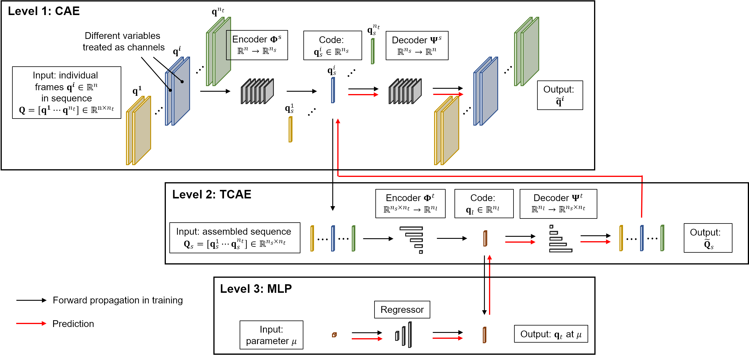
(a)

Figure 1: Schematic of new parameter prediction

For future state predictions, a TCN is used as the second level after the CAE. As shown in Fig. 2, TCN is used iteratively to predict future steps $\{\mathbf{q}_{s}(n_{t}+1;\mu),\dots,\mathbf{q}_{s}(n_{t}^{*};{\mu})\}$ subsequent to the output sequence $\mathbf{Q}_{s}(\mu)$ from the top level.

In either type of task, outputs at the bottom level are decoded to obtain the high-dimensional sequence at unseen global parameters and/or future states, as indicated by the red arrows in the diagrams.

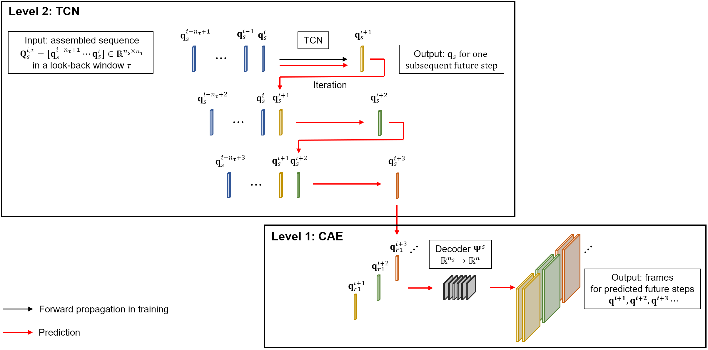
(a)

Figure 2: Schematic for future state prediction

3 Network Details

The proposed framework is comprised of multiple levels of neural networks. Following the order of integration, the basic network layers are introduced in Sec. 3.1, baseline network structures are introduced in Sec. 3.2, the constituent sub-level networks of the proposed framework are introduced in Sec. 3.3, pipelines for different tasks are described in Sec. 3.4, and additional details of the training process are provided in Sec. 3.5.

3.1 Layer structures

In this work, three types of layers are used, namely dense, convolutional and dilated convolutional layers.

3.1.1 Dense layer

The functional form of a dense layer is given by

$$f_{\text{dense}}(\mathbf{h};\mathbf{\Theta})=\sigma(g(\mathbf{h};\mathbf{\Theta})),$$ (1)

where $g(\mathbf{h};\mathbf{\Theta})\triangleq\mathbf{Wh+b}$ is a linear function, and $\sigma$ is an element-wise activation function, which can be nonlinear. The parameter $\mathbf{\Theta}\in\mathds{R}^{n_{g}\times(n_{h}+1)}$ consists of a bias part $\mathbf{b}\in\mathds{R}^{n_{g}}$, and a weight part $\mathbf{W}\in\mathds{R}^{n_{g}\times n_{h}}$. If all layers in a network are fully connected, the network is called a multilayer perceptron (MLP), which is the most basic type of neural network. In our work, nonlinear regression is performed using MLP with nonlinear activation functions.

3.1.2 Convolutional layers

A convolutional layer convolves filters with trainable weights with the inputs. Such filters are commonly referred to as convolutional kernels. In a convolutional neural network, the inputs and outputs can have multiple channels, i.e. multiple sets of variables defined on the same spatial grid such as the red, green and blue components in a digital colored image. For a convolutional layer with $n_{ci}$ input channels and $n_{co}$ output channels, the total number of convolutional kernels is $n_{k}=n_{ci}\times n_{co}$. Each kernel slides over the one input channel along all spatial directions, and dot products are computed at all sliding steps.The functional form of a convolutional layer is given by

$$f_{\text{conv}}(\mathbf{h};\mathbf{k})=\sigma((\mathbf{h}*\mathbf{k})).$$ (2)

In two-dimensional problems, at a sliding step centered at $(i_{x},i_{y})$, the 2D convolutional dot product of a kernel $\mathbf{k}\in\mathds{R}^{(2w_{x}+1)\times(2w_{y}+1)}$ on an input $\mathbf{x}$ is given by

$$(\mathbf{x}*\mathbf{k})_{i_{x},i_{y}}\triangleq\sum_{p=w_{x}}^{-w_{x}}{\sum_{q=w_{y}}^{-w_{y}}{\mathbf{x}_{i_{x}-p,i_{y}-q}\mathbf{k}_{p,q}}}.$$ (3)

Eq. (3) can be easily generalized for 1D or 3D as in Eq. (4) and (5)

$$(\mathbf{x}*\mathbf{k})_{i_{x}}\triangleq\sum_{p=w_{x}}^{-w_{x}}{\mathbf{x}_{i_{x}-p}\mathbf{k}_{p}},$$ (4)

$$(\mathbf{x}*\mathbf{k})_{i_{x},i_{y},i_{z}}\triangleq\sum_{p=w_{x}}^{-w_{x}}{\sum_{q=w_{y}}^{-w_{y}}{\sum_{r=w_{z}}^{-w_{z}}{\mathbf{x}_{i_{x}-p,i_{y}-q,i_{z}-r}\mathbf{k}_{p,q,r}}}}.$$ (5)

3.1.3 Dilated convolutional layer

In standard convolutions, the receptive field, i.e. the range in input that each output element is dependent on, growths linearly with the number of layers and the kernel size. This becomes a major disadvantage when applied to long sequential data, leading to a need for an extremely deep network or large kernels. As a solution, dilated convolution is performed in TCN.

The functional form of a dilated convolutional layer is given by

$$f_{\text{conv},d}(\mathbf{h};\mathbf{k})=\sigma((\mathbf{h}*_{d}\mathbf{k})).$$ (6)

In one dimension, the dilated convolution is a modified convolution operation with dilated connectivity between the input and the kernel, given by

$$(\mathbf{x}*_{d}\mathbf{k})_{i}\triangleq\sum_{p=0}^{w}{\mathbf{x}_{i-dp}\mathbf{k}_{p}},$$ (7)

where $d$ is called dilation order, and $w$ is the 1D kernel size. By increasing $d$ exponentially with the depth of the network, the receptive field also grows exponentially thus long sequences can be efficiently processed. A visualization of a TCN with multiple dilated convolutional layers of different dilation orders can be found in Ref. [65].

It should be realized that the dilation only affects the kernel connectivity and does not change the output shape, and hence, a sequence processed through it will remain a sequence. To compress the sequence dimension using TCN, the dilated convolution will be performed in a strided manner. In the strided dilated convolution, a stride of $wd$ is used, which means that the kernel will only slide through every $wd$ elements. Thus, any element between the first and last element convolved by the kernel will not be convolved with any other kernel. In contrast, the non-strided dilated convolution will slide through all elements. By using a strided convolution, the output size shrinks after being processed by every layer, and finally only one number is output for each channel.

3.2 Network structures

3.2.1 Feed-forward network

The feed-forward network is the simplest neural network structure, in which layers are interconnected in a feed-forward, i.e. sequential way. The computation in the $l$-th layer of a network takes the form

$$\mathbf{h}^{(l)}\triangleq f^{(l)}(\mathbf{h}^{(l-1)};\mathbf{\Theta}^{(l)}),$$ (8)

where $\mathbf{h}^{(0)}=\mathbf{x}\in\mathds{R}^{n_{x}}$ is the input layer, $\mathbf{h}^{(L)}=\tilde{\mathbf{y}}\in\mathds{R}^{n_{y}}$ is the output layer, and $\mathbf{\Theta}^{(l)}$ is a set of trainable parameters. Thus the $L$-layer feed-forward neural network can be expressed using a nonlinear function $\mathcal{F}:\mathds{R}^{n_{x}}\rightarrow\mathds{R}^{n_{y}}$ as

$$\tilde{\mathbf{y}}=\mathcal{F}(\mathbf{x};\mathbf{\Theta})\triangleq f^{(L)}\circ f^{(L-1)}\circ\cdots\circ f^{(2)}\circ f^{(1)}(\mathbf{x};\mathbf{\Theta}^{(1)}).$$ (9)

Eq. (9) is a serial process, thus if the feed-forward network is cut after the $l$-th layer $\mathbf{h}^{(l)}$ into two parts, with a leading part

$$\mathbf{\Phi}(\mathbf{x};\mathbf{\Theta}_{{\Phi}})\triangleq f^{(l)}\circ f^{(l-1)}\circ\cdots\circ f^{(2)}\circ f^{(1)}(\mathbf{x};\mathbf{\Theta}^{(1)}),$$

and a following part

$$\mathbf{\Psi}(\mathbf{h}^{(l)};\mathbf{\Theta}_{{\Psi}})\triangleq f^{(L)}\circ f^{(L-1)}\circ\cdots\circ f^{(l+2)}\circ f^{(l+1)}(\mathbf{h}^{(l)};\mathbf{\Theta}^{(l+1)}).$$

Then the output of the full network can be computed from two steps as

$$\mathbf{y}_{l}=\mathbf{\Phi}(\mathbf{x};\mathbf{\Theta}_{\phi}),$$ (10)

$$\mathbf{\tilde{y}}=\mathbf{\Psi}(\mathbf{y}_{l};\mathbf{\Theta}_{\psi}),$$ (11)

with $\mathbf{\Phi}:\mathds{R}^{n_{y}}\rightarrow\mathds{R}^{n^{(l)}}$ and $\mathbf{\Psi}:\mathds{R}^{n^{(l)}}\rightarrow\mathds{R}^{n_{y}}$.

3.2.2 Autoencoder

The intermediate variable $\mathbf{y}_{l}$ can be viewed as a set of latent representations for the full variable $\mathbf{y}$. When $\mathbf{y}_{l}$ is computed from the original input $\mathbf{x}$ using $\mathbf{\Phi}$, it is equal to $\mathbf{h}^{(l)}$ in the uncut network. Alternatively, if $\mathbf{y}_{l}$ can be obtained from other methods, the output $\mathbf{\tilde{y}}$ can be directly computed from it from the second step, Eq. (11) without the first step, Eq. (10).

An autoencoder is a type of feedforward network with two main characteristics: 1) The output is a reconstruction of the input, i.e. $\mathbf{x}\approx\mathbf{y}$; 2) Autoencoders - in general - assume a converging-diverging shape, i.e. the size of output first reduces then increases along the hidden layers. By cutting an autoencoder after its “bottleneck”, i.e. the hidden layer with the smallest size, the leading part $\mathbf{\Phi}$ will compress $\mathbf{y}$ into $\mathbf{y}_{l}$ with the dimension reduced from $n_{y}$ to $n^{(l)}$, and the following part $\mathbf{\Psi}$ will try to recover $\mathbf{y}$ from $\mathbf{y}_{l}$.

In an autoencoder, $\mathbf{\Phi}$ is called a encoder, and the transformation to the latent space is called encoding. $\mathbf{\Psi}$ is referred to as a decoder, and the reconstruction process is called decoding. The latent variable $\mathbf{y}_{l}$ is commonly referred to as code, and $n^{(l)}$ is called latent dimension.

3.3 Constituent levels

3.3.1 CAE

The CAE performs encoding-decoding along the spatial dimensions of the individual frames $\mathbf{q}(i;\mu)$. The encoding and decoding operations are expressed as

$$\mathbf{q}_{s}(i;\mu)=\mathbf{\Phi}_{s}(\mathbf{q}(i;\mu);\mathbf{\Theta}_{\phi s}),$$ (12)

$$\mathbf{\tilde{q}}(i;\mu)=\mathbf{\Psi}_{s}(\mathbf{q}_{s}(i;\mu);\mathbf{\Theta}_{\psi s}),$$ (13)

where the encoder $\mathbf{\Phi}_{s}:\mathds{R}^{n}\rightarrow\mathds{R}^{n_{s}}$ is parameterized by $\mathbf{\Theta}_{\phi s}$ and the decoder $\mathbf{\Psi}_{s}:\mathds{R}^{n_{s}}\rightarrow\mathds{R}^{n}$ is parameterized by $\mathbf{\Theta}_{\psi s}$.

The encoder $\mathbf{\Phi}_{s}$ begins with several convolution-pooling (Conv-pool) blocks. Each block consists of a 2D/3D convolutional layer with PReLU [70] activation, followed by a max-pooling layer that down-samples and reduces the size of the inputs. Zero-padding is applied to the convolutional layers to ensure consistent dimensionality between the inputs and outputs of the convolutional operation. The different variables in the flow field data are treated as different channels in the input layer (i.e. the convolutional layer in the first block). This treatment enables the network to process an arbitrary number of variables of interest without substantial change in structure. Following the Conv-pool operation, blocks are fully-connected (dense) layers with PReLU activation. Before the output layer (i.e. the last dense layer) of $\mathbf{\Phi}_{s}$, a flattening layer is added, which makes the output encoded latent variable $\mathbf{q}_{s}$ to be a flattened 1D variable.

The decoder $\mathbf{\Psi}_{s}$ takes the inverse structure of the encoder, with the Conv-pool blocks replaced by transposed convolution (Conv-trans) layers [71]. In the output layer of $\mathbf{\Psi}_{s}$, (i.e. the convolutional layer in the last transposed convolution layer), linear activation is used instead of the PReLU activation in other layers. A schematic of a sample CAE architecture with two Conv-pool blocks and two dense layers is given in Fig. 3.

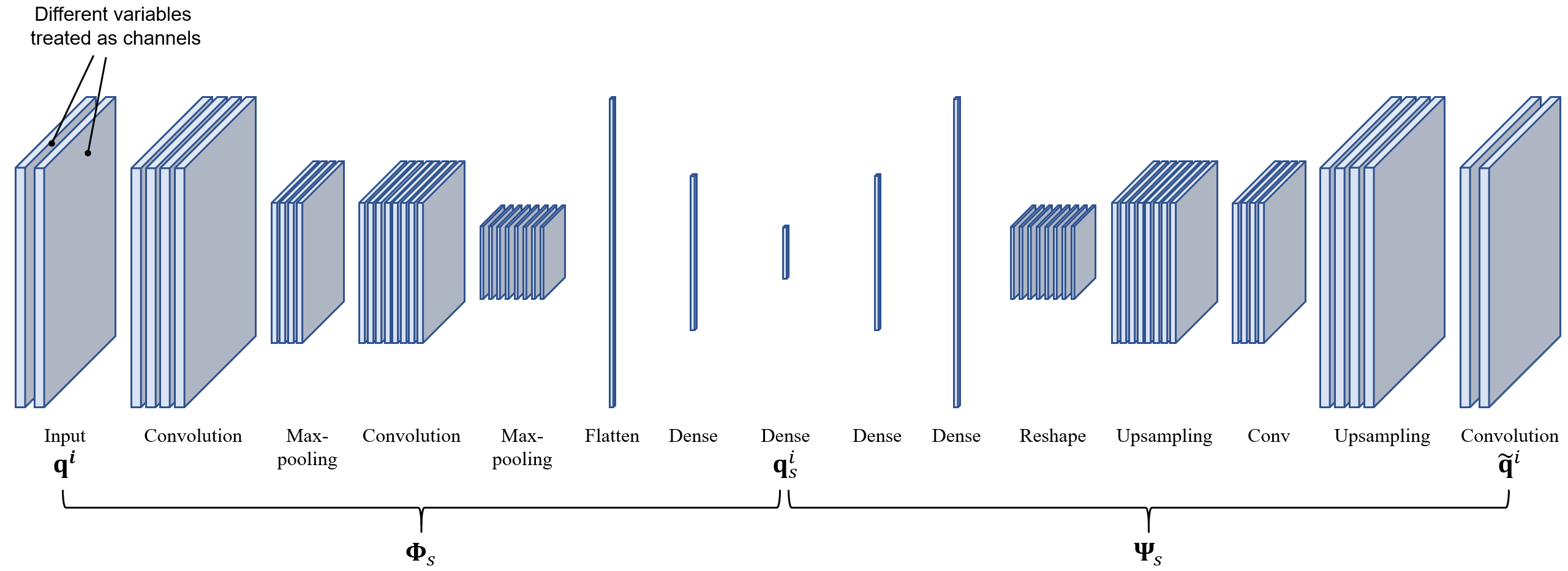
(a)

Figure 3: Sample CAE architecture. Leftmost and rightmost slabs represent a spatial field.

3.3.2 TCAE (for new parameter prediction)

In new parameter prediction, a TCAE is used to further compress the temporal dimension, such that each sequence $\mathbf{Q}_{s}(\mu)=[\mathbf{q}_{s}(1,\mu),\dots,\mathbf{q}_{s}({n_{t}},\mu)]\in\mathds{R}^{n_{s}\times n_{t}}$ is encoded into one set of latent variables $\mathbf{q}_{l}(\mu)\in\mathds{R}^{n_{l}}$. Thus, the total number of training samples for the TCAE equals the number of samples in parameter space $n_{\mu}$. For the sequence for a single parameter, the encoding and decoding operations are

$$\mathbf{q}_{l}(\mu)=\mathbf{\Phi}_{l}(\mathbf{Q}_{s}(\mu);\mathbf{\Theta}_{\phi l}),$$ (14)

$$\mathbf{\tilde{Q}}_{s}(\mu)=\mathbf{\Psi}_{l}(\mathbf{q}_{l}(\mu);\mathbf{\Theta}_{\psi l}),$$ (15)

The encoder $\mathbf{\Phi}_{l}:\mathds{R}^{n_{s}\times n_{t}}\rightarrow\mathds{R}^{n_{l}}$ is essentially a TCN by itself, where $\mathbf{Q}_{s}$ is processed as sequences of length $n_{t}$ for $n_{s}$ channels. For each of the channels, strided dilated convolutions are performed along the temporal dimension, and all steps in the sequence are integrated into one number at the last convolution layer. At this point, the size of the intermediate result is $n_{s}$ and the temporal dimension is eliminated. After the convolution layers, several dense layers with PReLU activation are used to further compress the intermediate variable into the output code $\mathbf{q}_{l}$. The decoder $\mathbf{\Psi}_{l}:\mathds{R}^{n_{l}}\rightarrow\mathds{R}^{n_{s}\times n_{t}}$ the inverted structure of $\mathbf{\Phi}_{l}$, but with non-strided dilated convolution layers and a dense layer with hyperbolic tangent (tanh) activation added to the end as the output layer. A schematic of a sample TCAE architecture with three convolution layers and two dense layers in $\mathbf{\Phi}_{l}$ is shown in Fig. 4.

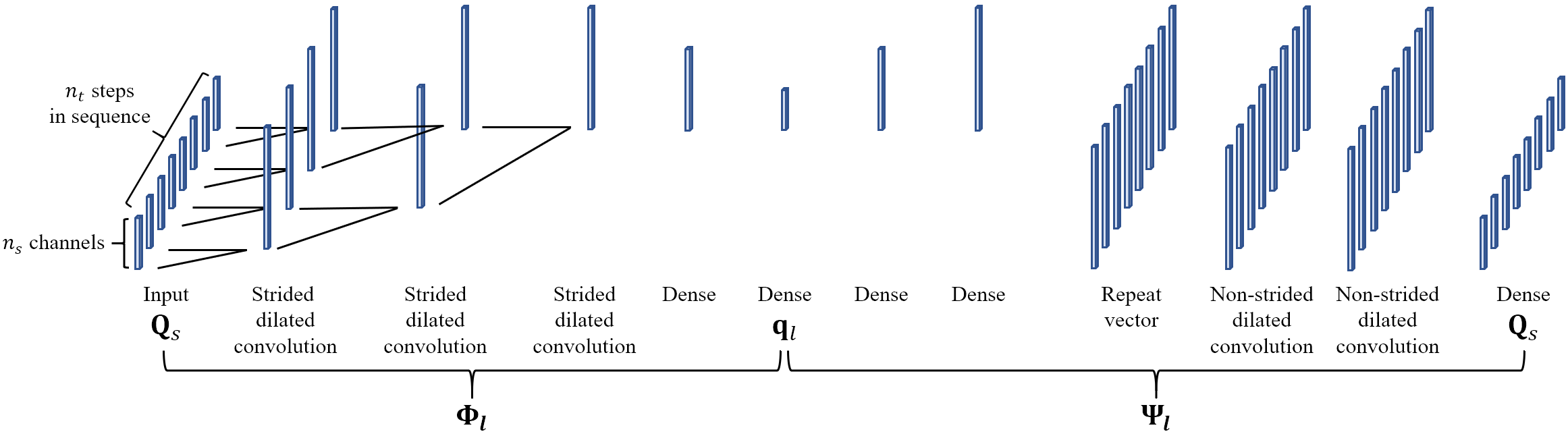
(a)

Figure 4: Sample TCAE architecture

3.3.3 MLP (for new parameter prediction)

The first two levels of encoding reduces the dimension of the data from $n\times n_{t}$ to $n_{l}$. The third level learns the mapping between the latent variable $\mathbf{q}_{l}(\mu)$ and the parameters $\mu$, and to predict $\mathbf{q}_{l}(\mu^{*})$ for unseen $\mu^{*}$. This is achieved by performing regression using a MLP with parameters $\mathbf{\Theta}_{R}$. The regression process is represented as

$$\tilde{\mathbf{q}}_{l}(\mu)=\mathcal{R}(\mu;\mathbf{\Theta}_{R}).$$ (16)

The MLP consists of multiple dense layers, where tanh activation is used in the last one and PReLU is used in the rest.

3.3.4 TCN (for future state prediction)

For future state prediction, the lower levels are different from that for prediction for new parameters. The necessity of the change of the lower-level network architecture is determined by the difference in training and prediction scopes for future state prediction from those for the previous task. More specifically, in this task, the goal is to afford flexibility in forecasting arbitrary number of future steps based on the temporal history patterns. Thus, the training data can be a sequence of arbitrary length instead of multiple fixed-length sequences at different global parameters. As a consequence of such differences, the aforementioned level 3 MLP is not required and the second level is replaced by a TCN serving as a future step predictor $\mathcal{P}:\mathds{R}^{n_{s}\times n_{\tau}}\rightarrow\mathds{R}^{n_{s}}$.

The time-series prediction using the TCN is performed iteratively. For each future step, the prediction is based on the temporal memory via a look-back window of $n_{\tau}$ steps, i.e. $n_{\tau}$ leading steps, $\mathbf{Q}_{s}(i;\mu;n_{\tau})=[\mathbf{q}_{s}(i-n_{\tau}+1;\mu),\dots,\mathbf{q}_{s}(i;\mu)]$, which is represented by

$$\tilde{\mathbf{q}}_{s}({i+1};\mu)=\mathcal{P}(\mathbf{Q}_{s}(i;\mu;\tau);\mathbf{\Theta}_{P}).$$ (17)

In general, two types of dynamics may exist in the temporal setting:

1. In the first type of dynamics, future states at a spatial point is completely determined by the temporal pattern at that point locally. This is analogous to standing waves. To process such dynamics, the TCN performs strided dilated convolutions along the temporal dimension.

2. The second type of dynamics involves spatial propagation, thus states of neighboring points are necessary in the prediction. This is analogous to traveling waves. For this type of dynamics, convolutions are performed along the latent dimension of $\mathbf{Q}_{s}$.

A schematic of a sample TCN architecture with convolutions along both spatial and temporal dimensions is shown in Fig. 5. It can be seen that the architecture of the predictor $\mathcal{P}$ is similar to the encoder $\mathbf{\Phi}_{l}$ in the TCAE described previously. The major difference between $\mathcal{P}$ and $\mathbf{\Phi}_{l}$ is in their outputs and training processes. Instead of being jointly trained with a decoder part and outputting an automatically encoded variable, the output of $\mathcal{P}$ has a more definitive meaning, which is the next latent variable subsequent to the input look-back sequence.

It should be noted that for simplicity and to demonstrate the primary characteristics in Fig. 5, the strided convolutions maintain the number of channels, and the non-strided convolutions do not affect the sequence length, which not necessary in the practical design of the TCN architecture. As demonstrated in Sec. 4, either type of convolution can be used along in the TCN when only one type of dynamics exist in the system.

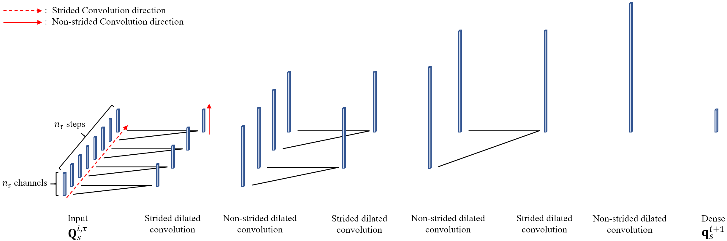
(a)

Figure 5: Sample TCN architecture

3.4 Framework pipeline

Table 1 summarizes the inputs and outputs of each component in the framework pipelines. It should be noted that scaling ($\mathcal{S}_{\sigma},\mathcal{S}_{\text{R}},\mathcal{S}_{\text{SR}}$) is also reflected in the same table, which is described in detail in Sec. 3.5.

Table 1: Network inputs/outputs

Network	Input	Output
$\mathbf{\Phi}_{s}$[a,b]	$\mathcal{S}_{\sigma}(\mathbf{q}(i;\mu))\in\mathds{R}^{n}$	$\mathbf{q}_{s}(i;\mu)\in\mathds{R}^{n_{s}}$
$\mathbf{\Psi}_{s}$[a,b]	$\mathbf{q}_{s}(i;\mu)\in\mathds{R}^{n_{s}}$	$\mathcal{S}_{\sigma}(\tilde{\mathbf{q}}(i;\mu))\in\mathds{R}^{n}$
$\mathbf{\Phi}_{l}$[a]	$\mathcal{S}_{\text{SR}}(\mathbf{Q}_{s}(\mu))\in\mathds{R}^{n_{s}\times n_{t}}$	$\mathbf{q}_{l}(\mu)\in\mathds{R}^{n_{l}}$
$\mathbf{\Psi}_{l}$[a]	$\mathbf{q}_{l}(\mu)\in\mathds{R}^{n_{l}}$	$\mathcal{S}_{\text{SR}}(\tilde{\mathbf{Q}}_{s}(\mu))\in\mathds{R}^{n_{s}\times n_{t}}$
$\mathcal{R}$[a]	$\mathcal{S}_{\text{R}}(\mu)\in\mathds{R}$	$\mathcal{S}_{\text{SR}}(\tilde{\mathbf{q}}_{l}(\mu))\in\mathds{R}^{n_{l}}$
$\mathcal{P}$[b]	$\mathcal{S}_{\text{SR}}(\mathbf{Q}_{s}(i;\mu;n_{\tau}))\in\mathds{R}^{n_{s}\times n_{\tau}}$	$\mathcal{S}_{\text{SR}}(\tilde{\mathbf{q}}_{s}(i+1;\mu))\in\mathds{R}^{n_{s}}$

• For new parameter prediction

• For future state prediction

3.4.1 New parameter prediction

As shown in the pipeline diagram, Fig. 1, the framework consists of three levels for this type of task, namely a CAE, a TCAE and a MLP. In the training process, $\mathbf{\Phi}_{s}$ and $\mathbf{\Psi}_{s}$ in the convolutional autoencoder are first trained jointly. Then by encoding the training data using the trained $\mathbf{\Phi}_{s}$, sequences $\mathbf{Q}_{s}$ are obtained and used to train $\mathbf{\Phi}_{l}$ and $\mathbf{\Psi}_{l}$. By encoding $\mathbf{Q}_{s}$ for different $\mu$ using the trained $\mathbf{\Phi}_{l}$, latent variables $\mathbf{q}_{l}$ are obtained, and used along with $\mu$ as the training data for $\mathcal{R}$.

To predict the dynamics for the desired parameter $\mu^{*}$, the spatio-temporally encoded latent variable is predicted by $\mathbf{q}_{l}(\mu^{*})=\mathcal{R}(\mu^{*})$, which is then sent into $\mathbf{\Psi}_{l}$ to obtain the sequence of spatially encoded latent variables $\mathbf{Q}_{s}(\mu^{*})=\mathbf{\Psi}_{l}(\mathbf{q}_{l}(\mu^{*}))$. Finally, the frames in the predicted flow field sequence are decoded as $\mathbf{q}(i;\mu^{*})=\mathbf{\Psi}_{s}(\mathbf{q}_{s}(i;\mu^{*}))$.

3.4.2 Future state prediction

For future state prediction, the training process shares the same initial step as in the previous task, which is the training of the level 1 convolutional autoencoder. After the sequence $\mathbf{Q}_{s}(\mu)$ is obtained, the training of $\mathcal{P}$ is performed by taking each step $\mathbf{q}_{s}(i;\mu)$ with $i>n_{\tau}$ and its corresponding look-back window $\mathbf{Q}_{s}(i-1;n_{\tau};\mu)$ as the training data.

As shown in Fig. 2, in the prediction for future states of a given sequence, the look-back window for the last known time step $\mathbf{Q}_{s}(n_{t};n_{\tau};\mu)$ is used as the input, and the spatially encoded latent variable for the subsequent time step is predicted using $\mathbf{q}_{s}({n_{t}+1};\mu)=\mathcal{P}(\mathbf{Q}_{s}(n_{t};n_{\tau};\mu)$). The corresponding future state is decoded by $\mathbf{q}({n_{t}+1};\mu)=\mathbf{\Psi}_{s}(\mathbf{q}_{s}({n_{t}+1};\mu))$. By performing such predictions iteratively, multiple future steps can be predicted.

3.5 Training

It is noted in both of the architectures considered above, the training for each level is performed sequentially. After the training of an autoencoder, the encoded variables generated from the trained encoder part serve as the ground truth for the target output for the following network. The goal for each individual training process is to minimize a loss function $\mathcal{L}(\mathbf{\Theta})$ by optimizing the network parameters $\mathbf{\Theta}$. In this work $\mathcal{L}$ is primarily based on the mean squared error (MSE), which is defined on the target output $\mathbf{y}$ and the prediction $\tilde{\mathbf{y}}(\mathbf{\Theta})$ as

$$\text{MSE}(\mathbf{y},\tilde{\mathbf{y}}(\mathbf{\Theta}))=\frac{({\tilde{\mathbf{y}}-\mathbf{y}})^{T}({\tilde{\mathbf{y}}-\mathbf{y}})}{n_{y}},$$ (18)

where $n_{y}$ is the degrees of freedom in $\mathbf{y}$.

To alleviate overfitting, a penalty on $\mathbf{\Theta}$ is added as a regularization term to $\mathcal{L}$. Common choices of regularization include the $\ell_{1}$-norm and $\ell_{2}$-norm. In this work, the latter is used and the final expressions for the loss function is given by

$$\mathcal{L(\mathbf{\Theta})}=\text{MSE}(\mathbf{y},\tilde{\mathbf{y}}(\mathbf{\Theta}))+\lambda\left\lVert\mathbf{\Theta}\right\rVert_{2},$$ (19)

where $\lambda$ is a penalty coefficient. The optimal parameters $\mathbf{\Theta}^{*}$ to be trained are then

$$\Theta^{*}=\underset{\Theta}{\operatorname{arg}\,\operatorname{min}}\;\mathcal{L(\mathbf{\Theta})}.$$ (20)

Back propagation is used to optimize the network parameters iteratively based on the gradient $\nabla_{\mathbf{\Theta}}\mathcal{L}$. There are numerous types of gradient-based optimization methods, and in this work Adam optimizer [72] is used.

To accelerate training, three types of feature scaling are applied, namely standard deviation scaling $\mathcal{S}_{\sigma}$, minimum-maximum range scaling $\mathcal{S}_{\text{R}}$ and shifted minimum-maximum range scaling $\mathcal{S}_{\text{SR}}$. With the original input or output feature, e.g. $\mathbf{q}$ or $\mu$, denoted by $x$, the scaling operations are given by

$$\mathcal{S}_{\sigma}(x)=\frac{x-\text{mean}(x_{train})}{\sigma(x_{train})}.$$ (21)

$$\mathcal{S}_{\text{R}}(x)=\frac{x-\text{min}(x_{train})}{\text{max}(x_{train})-\text{min}(x_{train})}.$$ (22)

$$\mathcal{S}_{\text{SR}}(x)=\frac{x-\text{min}(x_{train})}{\text{max}(x_{train})-\text{min}(x_{train})}-0.5.$$ (23)

The use of the scaling methods in different parts of the framework is summarized in Table 1.

4 Numerical tests

In this section, numerical tests are performed on three representative problems of different dimensions and characteristics of dynamics. These test cases have proven to be challenging for traditional POD-based model reduction techniques. The advection of a half cosine wave is used as a simplified illustrative problem in 4.1, to aid the understanding of a few concepts of the framework. In A, numerical tests are performed with the POD at the top-level to provide a comparison between POD- and CAE-based methods for reference. A sensitivity study of latent dimensions in the autoencoders is provided in B.

Besides MSE (Eq. (18)), the relative absolute error (RAE) is taken as another criterion to assess the accuracy of the predictions. For simplicity, we will use $\epsilon_{\text{MSE}}^{y}=\text{MSE}(\mathbf{y},\tilde{\mathbf{y}})$ and $\epsilon_{\text{RAE}}^{y}=\text{RAE}(\mathbf{y},\tilde{\mathbf{y}})$ to denote the two types of errors for variable $y$. The latter is given by

$$\text{RAE}(\mathbf{y},\tilde{\mathbf{y}})=\frac{\overline{|\tilde{\mathbf{y}}-\mathbf{y}|}}{\text{max}(|\mathbf{y}|)},$$ (24)

where $\overline{|\tilde{\mathbf{y}}-\mathbf{y}|}$ is the mean of the absolute value of $\tilde{\mathbf{y}}-\mathbf{y}$, and $\text{max}(|\mathbf{y}|)$ is the maximum of the absolute value of $\mathbf{y}$ over the entire computational domain. It should be noted that in the evaluation of subsequent levels, the encoded variables from the preceding levels are taken as the truth. Training and testing convergence is reported in  C.

For a reduced order prediction method aimed at many-query applications, computational efficiency is another important aspect in the framework performance metrics. In this work, all numerical tests are performed using one NVIDIA Tesla P100 GPU and timing results are provided accordingly.

4.1 Linear advection

The advection of a half cosine wave is used to illustrate encoding-decoding and future state prediction processes in a simplified setting. In this problem, a one-dimensional spatial discretization of 128 grid nodes is used. Initially the half cosine wave, spanning 11 grid nodes, is centered at the 15th grid node, and translates 100 grid nodes in 25 frames at a constant advection speed of 4 nodes/frame without any deformation. The initial frame, the last frame in training, $i=5$, and the final frame to be predicted, $i=25$, are shown in Fig. 7. In this test, it is assumed that only the first 5 frames of data are available in the training stage, and prediction is performed for the next 20 frames. Errors for the final prediction and different stages of output are summarized in Table 3.

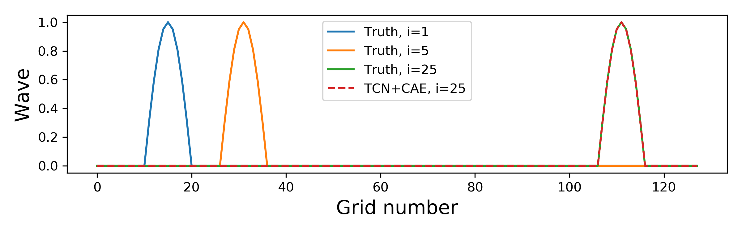
Figure 6: Linear advection: true and predicted profiles

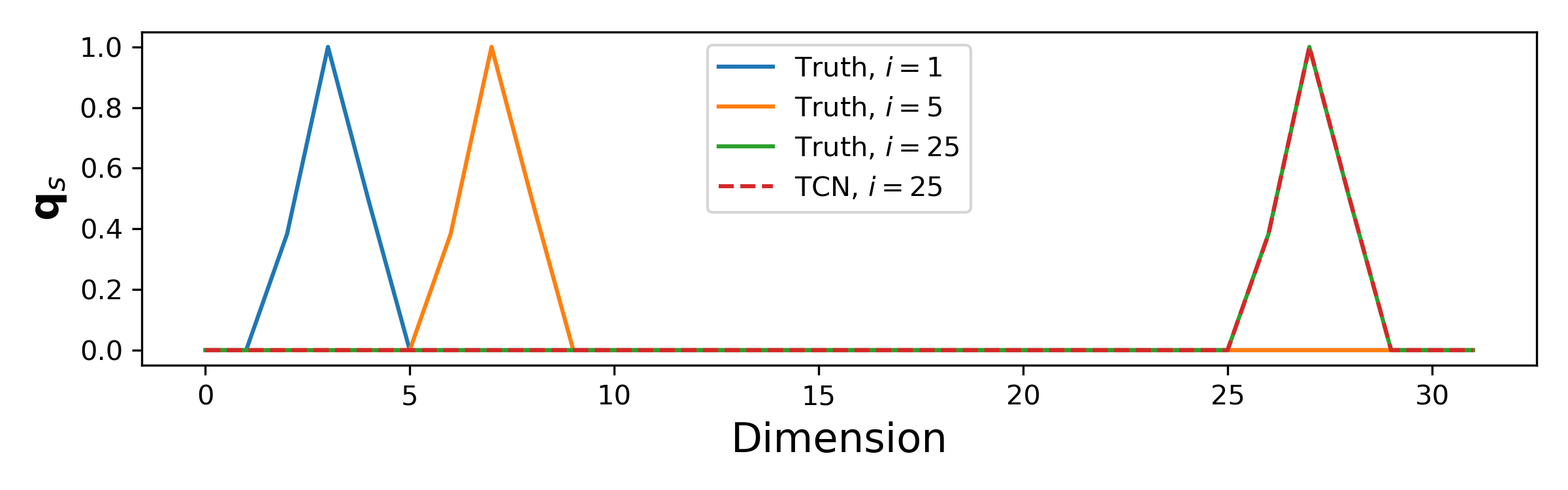
Figure 7: Linear advection: $\mathbf{q}_{s}$ profiles

Table 2: Linear advection: network architectures

$\mathbf{\Phi}_{s}$
Layer	Input	Convolution	Convolution	Convolution	Flatten (Output)
Output shape	$128\times 1$	$64\times 32$	$32\times 64$	$32\times 1$	32
$\mathbf{\Psi}_{s}$
Layer	Input	Reshape	Conv-trans	Conv-trans	Conv-trans (Output)
Output shape	32	$32\times 1$	$32\times 64$	$64\times 32$	$128\times 1$

(a) CAE

Layer	Input	2-layer TCN block	Convolution	Flatten (Output)
Output shape	$32\times 2$	$32\times 32$	$32\times 1$	32

(b) TCN

A simple CAE with three convolutional layers is first used for spatial compression, so that the prediction is performed for 32 latent degrees of freedom instead of the original 128 degrees of freedom for the spatially discretized variable. The detailed CAE architecture is provided in Table 2a. The latent variable $\mathbf{q}_{s}=\mathbf{\Phi}_{s}(\mathbf{q})$ is shown in Fig. 7 for the same time instances as in Fig. 7. It can be seen that the original half cosine wave is transformed into a triangular wave consisting of two linear halves. From Table 3 it can be seen that the CAE reconstruction shows the same error numbers in both the training and testing stages, which shows that the CAE is able to represent the cosine wave to the same precision regardless of its position in the domain due to its conservation in shape.

A TCN future step predictor $\mathcal{P}$ is used as the second level to predict $\mathbf{q}_{s}$ for future steps. As listed in Table 2b, $\mathcal{P}$ consists of a TCN block with 32 channels and a convolutional layer that reduces the 32 channels into a single output channel which would be the future step of $\mathbf{q}_{s}$. The TCN block consists of two dilated 1D convolutional layers with dilation orders $d=1,2$. As a propagation problem, both convolution layers are non-strided and operates along the latent dimension. While a single look-back step is sufficient, to make the case more representative for more complex problems, a look-back window of $n_{\tau}=2$ is used. Thus the input dimension to the TCN is $n\times n_{\tau}=32\times 2$.

With $n_{\tau}=2$, the 5 training frames are grouped into 3 training samples for TCN, i.e. the 1st and 2nd frames as the input, the 3rd frame as the target output; the 2nd and 3rd frames as the input, the 4th frame as the target output, etc. After the prediction for a new frame $i$, the second frame in the original look-back window, i.e. frame $i-1$, is used as the first frame in the new window for the prediction of frame $i+1$, and the predicted frame $i$ is used as the second frame in the new window. After 20 iterations, the predicted final frame of $\mathbf{q}_{s}$ for $i=25$ is obtained. As listed in Table 3, the error introduced by the TCN (i.e. in the prediction for $\mathbf{q}_{s}$) is negligible compared with that by the CAE. Thus the predicted future states $\mathbf{q}^{*}=\mathbf{\Psi}_{s}(\tilde{\mathbf{q}}_{s})$ shows an RAE of 0.04%, which is dominated by the CAE reconstruction error. The predicted final step $i=25$ is shown in Fig. 7.

Table 3: Linear advection: errors for different stages of output

Stage	Truth	Output	RAE	MSE
Training (frames 1 to 5)	$\mathbf{q}$	$\mathbf{\tilde{q}}=\mathbf{\Psi}_{s}(\mathbf{\Phi}_{s}(\mathbf{q}))$	0.04%	$1.910-5$
	$\mathbf{q}_{s}=\mathbf{\Phi}_{s}(\mathbf{q})$	$\tilde{\mathbf{q}}_{s}=\mathcal{P}(\mathbf{Q}_{s})$	$3.010-8$	$1.410-14$
Testing (frames 6 to 25)	$\mathbf{q}$	$\mathbf{\tilde{q}}=\mathbf{\Psi}_{s}(\mathbf{\Phi}_{s}(\mathbf{q}))$	0.04%	$1.910-5$
	$\mathbf{q}_{s}=\mathbf{\Phi}_{s}(\mathbf{q})$	$\tilde{\mathbf{q}}_{s}=\mathcal{P}(\mathbf{Q}_{s})$	$1.610-6$	$9.910-11$
	$\mathbf{q}$	$\tilde{\mathbf{q}}^{*}=\mathbf{\Psi}_{s}(\tilde{\mathbf{q}}_{s})$	0.04%	$1.910-5$

4.2 Discontinuous compressible flow

The Sod shock tube [73] is a classical test and studies the propagation of a rarefaction wave, a shock wave and a discontinuous contact surface initiated by a discontinuity in pressure at the middle of a one dimensional tube filled with ideal gas. This flow is governed by the one dimensional Euler equations of gas dynamics [74]. The standard initial left and right states are $P_{L}=1,\rho_{L}=1,U_{L}=0,P_{R}=0.1,\rho_{R}=0.125,U_{R}=0$, where $P,\rho,U$ are the density, pressure and velocity respectively. A detailed description of the exact solution for the problem can be found in [74].

In this numerical test, the evolution of $P,\rho,U$ will be predicted in the the time interval 0.1 to 0.25 s based on the dynamics before 0.1 s. The profiles are plotted in Fig. 8 for several time instances for $0\leq t\leq 0.25$ s. The ground truth are obtained by mapping the exact solution onto a 200-point 1D grid with a temporal discretization of 35 steps per 0.1 s. Such propagation problems are considered challenging from the perspective of model reduction [75] because the dynamics in prediction stage is not covered in training, leading to failure for ROMs based on global bases. Errors for different stages of output in the proposed framework are summarized in Table 5.

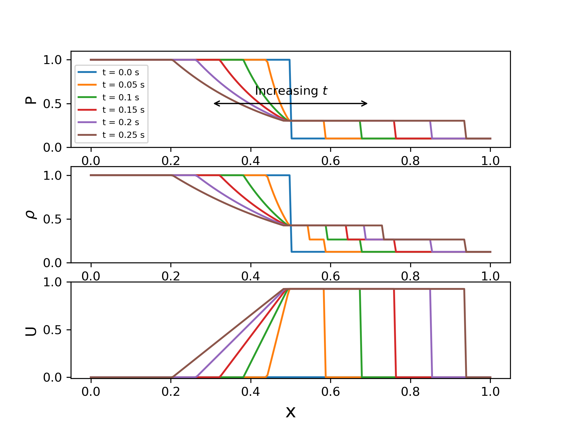
Figure 8: Discontinuous compressible flow: Profiles of pressure, density and velocity.

Table 4: Discontinuous compressible flow: network architectures

$\mathbf{\Phi}_{s}$
Layer	Input	Convolution	Convolution	Flatten (Output)
Output shape	$200\times 3$	$200\times 128$	$200\times 1$	200
$\mathbf{\Psi}_{s}$
Layer	Input	Reshape	Conv-trans	Conv-trans (Output)
Output shape	200	$200\times 1$	$200\times 128$	$200\times 3$

(a) CAE

Layer	Input	2-layer TCN block	2-layer TCN block	Convolution	Flatten (Output)
Output shape	$200\times 2$	$200\times 200$	$200\times 400$	$200\times 1$	200

(b) TCN

Due to the relatively small grid size an aggressive spatial compression is not necessary, thus no pooling or dense layer is used in the CAE. The detailed CAE architecture is given in Table 4a. The reconstructed variables $\mathbf{\tilde{q}}=\mathbf{\Psi}_{s}(\mathbf{\Phi}_{s}(\mathbf{q}))$ is shown at the final time step $t=0.25$ s in Fig. 10. This result is effectively an estimate of the lower bound of the error in the prediction case. For the same step, $\mathbf{q}_{s}$ is present in Fig. 10. It can be seen that the encoded variable behaves similarly to a scaled variation of $\rho$, which contains the most complex dynamics with two discontinuities among the three variables studied. This illustrates an efficient dimension reduction by reducing the number of variables in the CAE, even without any pooling operation.

A short look-back window of $n_{\tau}=2$ is used as in the previous demonstration case, but for this more complicated propagation problem, the size of TCN is significantly increased. $\mathcal{P}$ consists of two TCN blocks with 200 and 400 channels respectively, followed by one convolutional layer that reduces the 400 channels of the second TCN block into one output channel, which would be the future step of $\mathbf{q}_{s}$. Each of the TCN blocks consist of two non-strided dilated 1D convolutional layers with dilation orders $d=1,2$. The detailed architecture of $\mathcal{P}$ is given in Table 4b. 53 iterative prediction steps for $\mathbf{q}_{s}$ are performed for $0<t\leq 0.25$ s, and the predicted future states are decoded from them. The predicted profiles at $t=0.25$ s for $\mathbf{q}$ and $\mathbf{q}_{s}$ are present in Fig. 10 and Fig. 10. The RAE in the prediction for the three variables are all below 0.35%.

Table 5: Discontinuous compressible flow: errors for different stages of output

Stage	Truth	Output	RAE	MSE
Training ($0\leq t\leq 0.1$ s)	$\mathbf{q}\,(P/\rho/U)$	$\mathbf{\tilde{q}}\,(P/\rho/U)=\mathbf{\Psi}_{s}(\mathbf{\Phi}_{s}(\mathbf{q}))$	0.03%/0.01%/0.03%	$1.210-6$/$2.410-7$/$1.610-6$
	$\mathbf{q}_{s}=\mathbf{\Phi}_{s}(\mathbf{q})$	$\tilde{\mathbf{q}}_{s}=\mathcal{P}(\mathbf{Q}_{s})$	0.008%	$1.210-6$
Testing ($0.1<t\leq 0.25$ s)	$\mathbf{q}\,(P/\rho/U)$	$\mathbf{\tilde{q}}\,(P/\rho/U)=\mathbf{\Psi}_{s}(\mathbf{\Phi}_{s}(\mathbf{q}))$	0.10%/0.05%/0.09%	$5.410-6$/$1.510-6$/$5.110-6$
	$\mathbf{q}_{s}=\mathbf{\Phi}_{s}(\mathbf{q})$	$\tilde{\mathbf{q}}_{s}=\mathcal{P}(\mathbf{Q}_{s})$	0.22%	$6.510-5$
	$\mathbf{q}\,(P/\rho/U)$	$\tilde{\mathbf{q}}^{*}\,(P/\rho/U)=\mathbf{\Psi}_{s}(\tilde{\mathbf{q}}_{s})$	0.32%/0.34%/0.31%	$7.610-5$/$1.610-4$/$8.810-5$

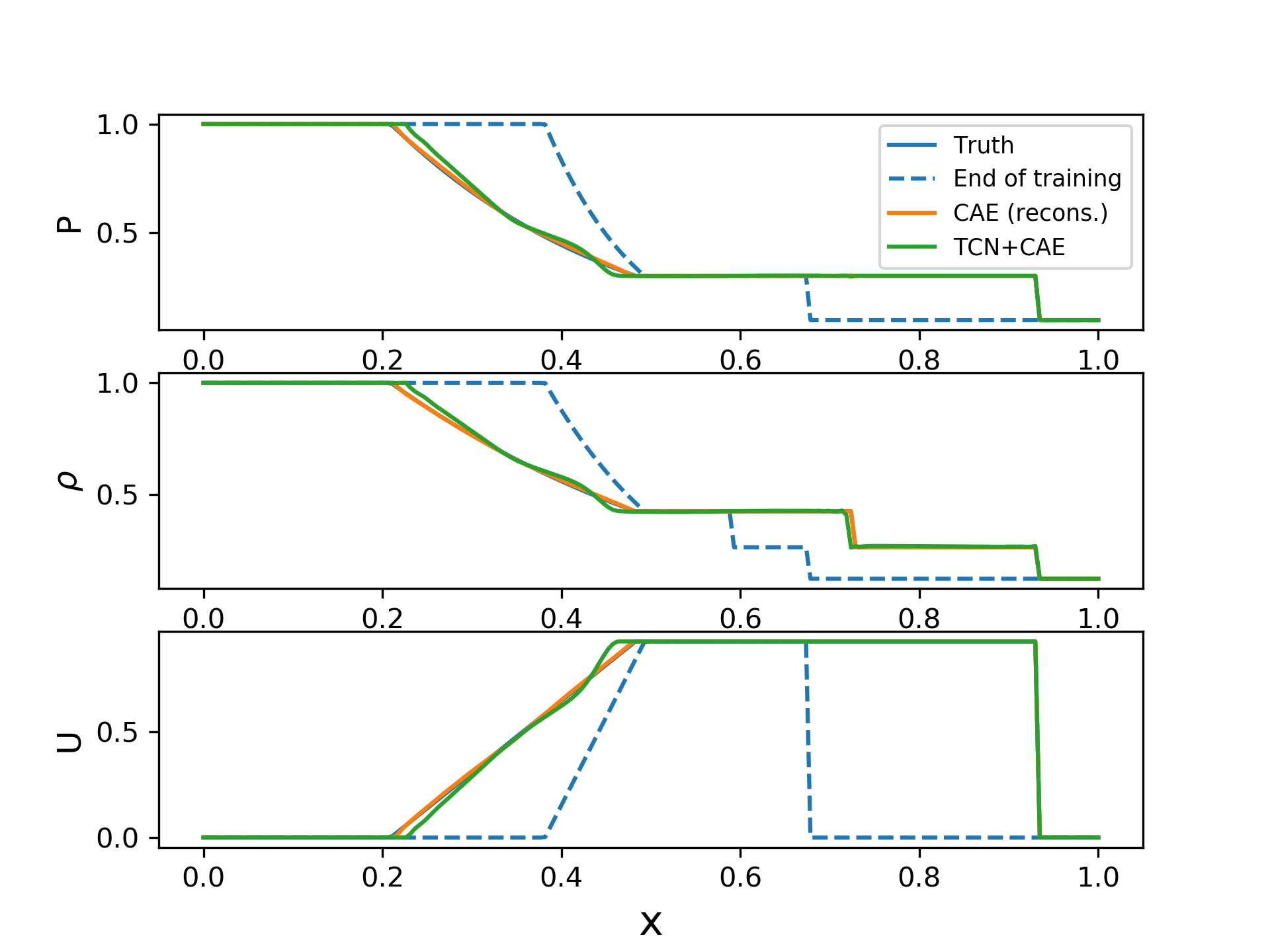
Figure 9: Discontinuous compressible flow: reconstructed (recons.) and predicted profiles for $t=0.25$ s

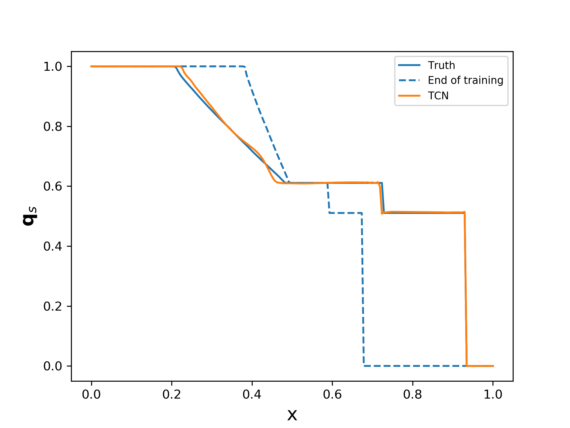
Figure 10: Discontinuous compressible flow: Latent variables $\mathbf{q}_{s}$ for $t=0.25$ s

The computing time by different parts of the framework in training and prediction is listed in Table 6. The total prediction time for 0.15 s of propagation is 0.6 s.

Table 6: Discontinuous compressible flow: computing time

Training
Component	CAE	TCN	Total
Training epochs	1000	2000	-
Computing time (s)	171	166	337
Prediction (53 frames)
Component	$\mathbf{\Psi}_{s}$	TCN	Total
Computing time (s)	0.48	0.12	0.60

4.2.1 Impact of training sequence length

To evaluate the sensitivity of the predictions on the amount of training data, the above TCN is re-trained on training sequences of different length $n_{t}$, ranging from 20 to 40 frames. The comparison is performed on 20 iterative future prediction steps.

The RAE for TCN training and prediction, as well as the decoded result using $\mathbf{\Phi}_{s}$ is shown in Fig. 11. Sample prediction results are given in Fig. 12. It is seen that at $n_{t}=20$, the TCN is unable to provide an accurate future state prediction. The error decreases rapidly with increasing number of training snapshots, and starts to saturate after $n_{t}=30$. This behavior was observed in other levels of the framework, illustrating the importance of sufficient training data as can be expected of data-driven frameworks.

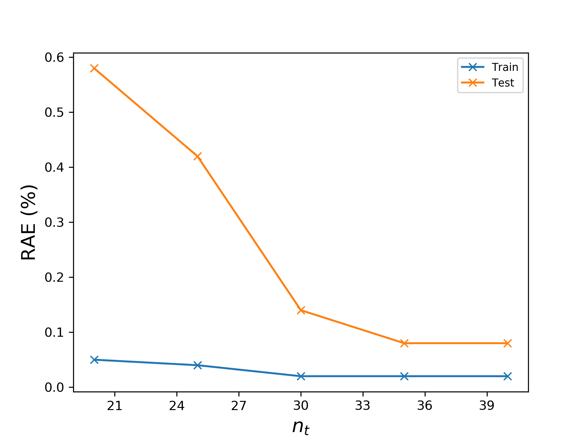
(a) TCN training and prediction

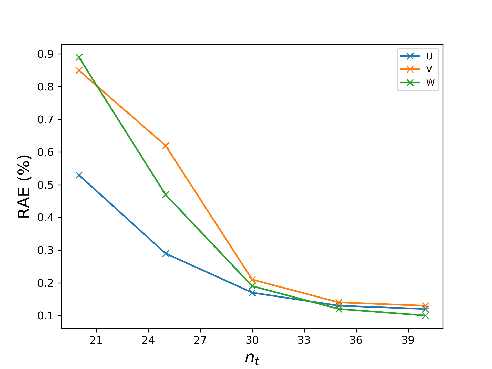
(b) Decoded variables from TCN prediction

Figure 11: Discontinuous compressible flow: sensitivity of RAE to number of training samples $n_{t}$

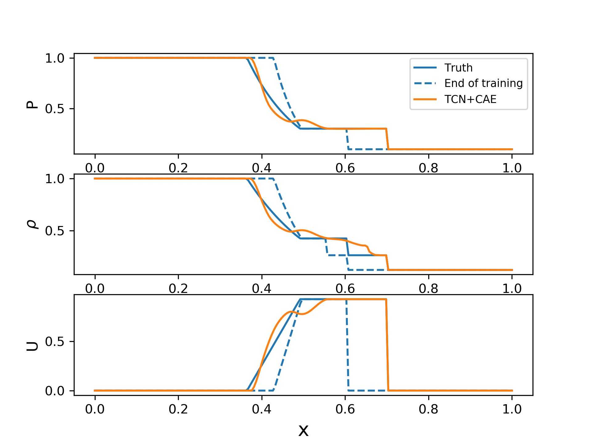
(a) $n_{t}=20$

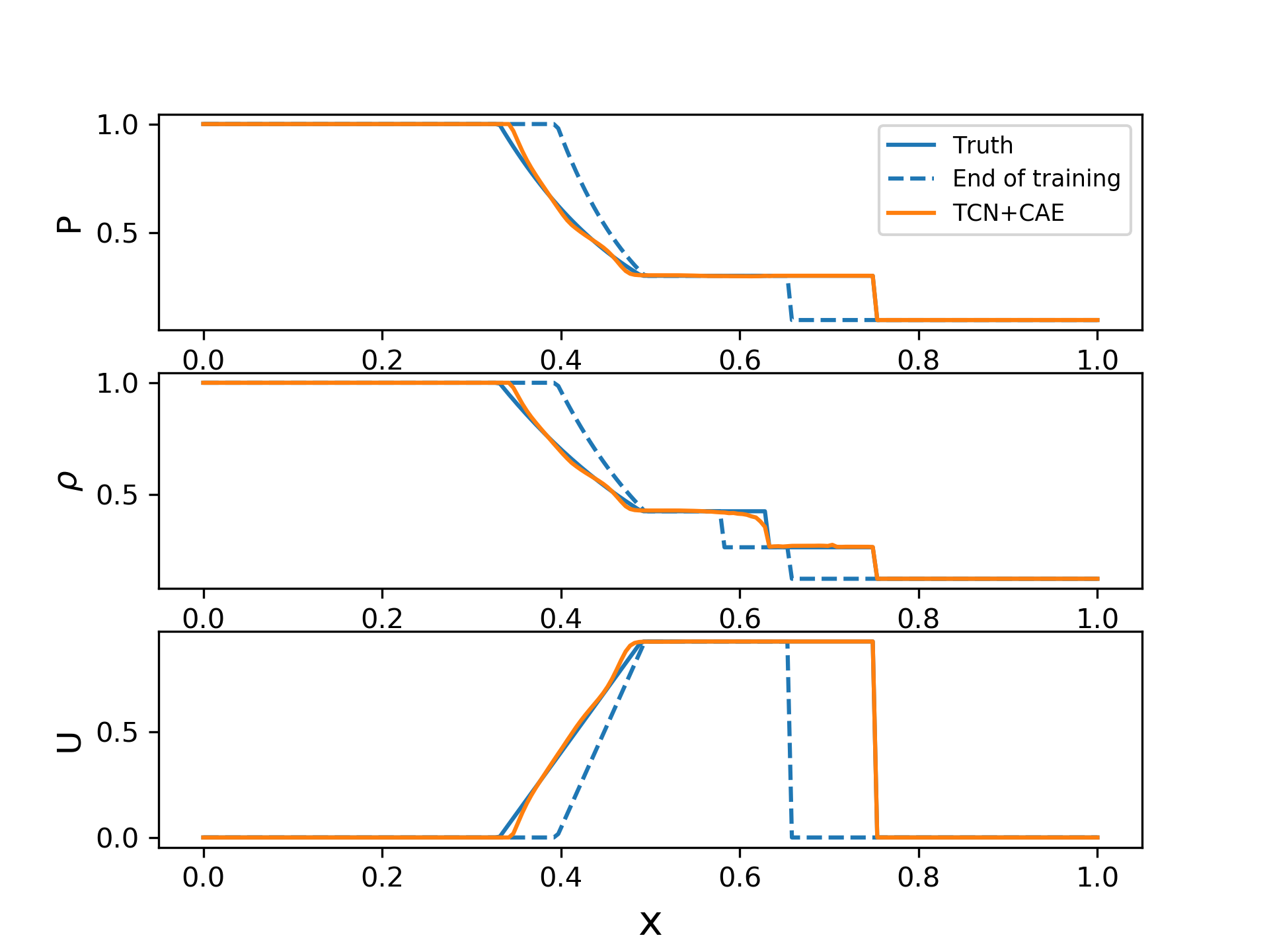
(b) $n_{t}=30$

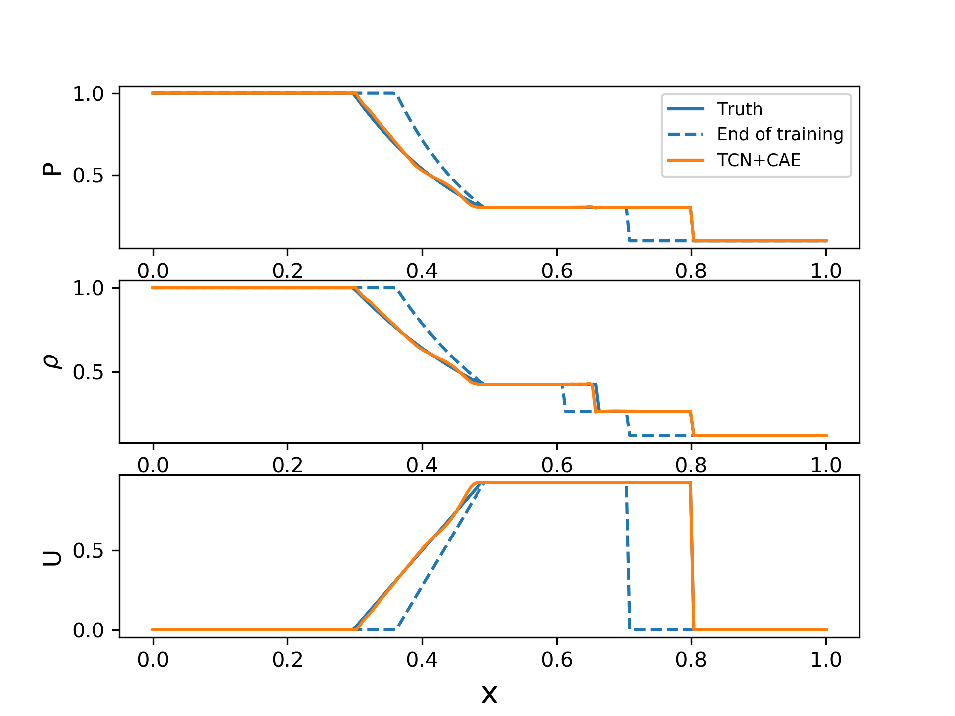
(c) $n_{t}=40$

Figure 12: Discontinuous compressible flow: sensitivity of (20-step) prediction result to number of training samples $n_{t}$

4.3 Transient flow over a cylinder

In this test case, transient flow over a cylinder is considered. Despite the simple two-dimensional flow configuration, the complexity is characterized by the evolution of the flow from non-physical, attached flow initial conditions conditions to boundary layer separation and consequently, vortex shedding. The flow dynamics is determined by a global parameter, the Reynolds number $Re$, defined as

$$Re=\frac{U_{\infty}D}{\nu},$$ (25)

where $U_{\infty}$ is the inflow velocity, $D$ is the diameter of the cylinder and $\nu$ is the viscosity of the fluid.

The domain of interest spans $20D$ in the x-direction and $10D$ in y-direction. Solution snapshots of the incompressible Navier–Stokes equations are interpolated onto a $384\times 192$ uniform grid. The $x$-velocity $U$ and $y$-velocity $V$ are chosen as the variables of interest.

For this test case, a parametric prediction is first performed for a new $Re$, and a future state prediction is then appended to the predicted sequence. Errors for different stages of output are summarized in Table 8.

4.3.1 New parameter prediction

In this task, the training data consists of 6 unsteady flow field sequences corresponding to $Re_{\text{train}}=\{125,150,175,225,250,275\}$, and prediction is performed for $Re_{\text{test}}=200$. All sequences are generated from the same steady initial condition corresponding to $Re=20$, each lasting 2500 frames. The sequence length is chosen on purpose to cover the transition to LCO. Depending on $Re$, vortex shedding frequencies are different and the transition to LCO occurs at different rates. A sample contour of flow field is given in Fig. 13a. To better illustrate the transition process, as well as the difference between different $Re$, a point monitor is placed $1D$ downstream of the center of the cylinder. The velocity at this location is shown for two training parameters $Re=\{125,275\}$ and the testing parameter $Re=200$ in Fig. 15.

Table 7: Transient flow over a cylinder: network architectures

$\mathbf{\Phi}_{s}$
Layer	Input	Conv-pool	Conv-pool	Conv-pool	Conv-pool	Flatten	Dense (Output)
Output shape	$384\times 192\times 2$	$192\times 96\times 32$	$96\times 48\times 64$	$48\times 24\times 128$	$24\times 24\times 256$	147456	60
$\mathbf{\Psi}_{s}$
Layer	Input	Dense	Reshape	Conv-trans	Conv-trans	Conv-trans	Conv-trans (Output)
Output shape	60	147456	$24\times 24\times 256$	$48\times 24\times 128$	$96\times 48\times 64$	$192\times 96\times 32$	$384\times 192\times 2$

(a) CAE

$\mathbf{\Phi}_{l}$
Layer	Input		12-layer TCN block	Dense	Dense (Output)
Output shape	$60\times 2500$		200	100	100
$\mathbf{\Psi}_{l}$
Layer	Input	Dense	Dense	Repeat vector	12-layer TCN block (Output)
Output shape	100	100	200	$200\times 2500$	$60\times 2500$

(b) TCAE

Layer	Input	Dense	Dense	Dense (Output)
Output shape	1	32	256	100

(c) MLP

Layer	Input	5-layer TCN block	Dense (Output)
Output shape	$60\times 150$	$200$	$60$

(d) TCN

The top level CAE contains 4 Conv-pool blocks and 1 dense layer in the encoder, with encoded latent dimension $n_{s}=60$. The decoder assumes a symmetric shape, and the detailed CAE architecture is provided in Table 7a. A comparison between the input flow field and the reconstructed variables $\mathbf{\tilde{q}}=\mathbf{\Psi}_{s}(\mathbf{\Phi}_{s}(\mathbf{q}))$ for the last frame is provided in Fig. 13a and 13b. The point monitored variable history for the reconstructed variable is plotted in Fig. 15. The maximum reconstruction RAE is 0.19%.

The spatially encoded variable for the training sequences $\mathbf{q}_{s}(Re_{train})=\mathbf{\Phi}_{s}(\mathbf{Q}(Re_{train}))$ is used to train the TCAE. The TCN block in $\mathbf{\Phi}_{l}$ of the TCAE contains 12 dilated convolutional layers, with uniform kernel size $k=10$ and sequential dilation orders $d=1,2,2^{2},\dots,2^{10},2^{11}$. Two dense layers are appended after the TCN block, and the encoded latent dimension is $n_{l}=100$. $l_{2}$ regularization with a penalty factor $\lambda=$110-8$$ is used in the loss function. The history of the first channel of the true and TCAE reconstructed $\mathbf{Q}_{s}$ is plotted in Fig. 17.

To learn the mapping between $Re$ and $\mathbf{q}_{l}$, a MLP of 3 dense layers is used. The detailed architecture of the MLP is given in Table 7c. The predicted $\mathbf{q}_{l}^{*}=\mathcal{R}(Re=200)$ is compared with the truth in Fig. 17. The error in $\mathbf{q}_{l}^{*}$ is around 1%. $\mathbf{\Psi}_{l}$ and $\mathbf{\Psi}_{s}$ are then used to decode the final prediction for the flow field. The first channel of the intermediate output $\mathbf{Q}_{s}^{*}=\mathbf{\Psi}_{l}(\mathbf{q}_{l}^{*})$ is compared to the truth in Fig. 17. The RAE in the velocity components for the final output $\mathbf{Q}^{*}=\mathbf{\Psi}_{s}(\mathbf{Q}_{s}^{*})$ is below 1.4%. The last frame of the solution is contoured in Fig. 13c, and the point monitor history is shown in Fig. 15.

(a) Truth

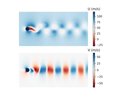
(b) CAE reconstruction

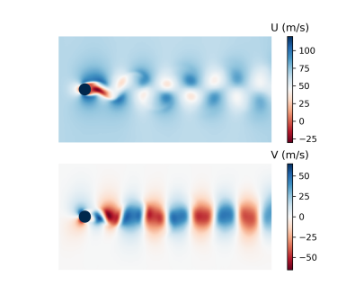
(c) MLP+TCAE+CAE

Figure 13: Transient flow over a cylinder new parameter prediction: flow field contours for $i=2500,Re=200$

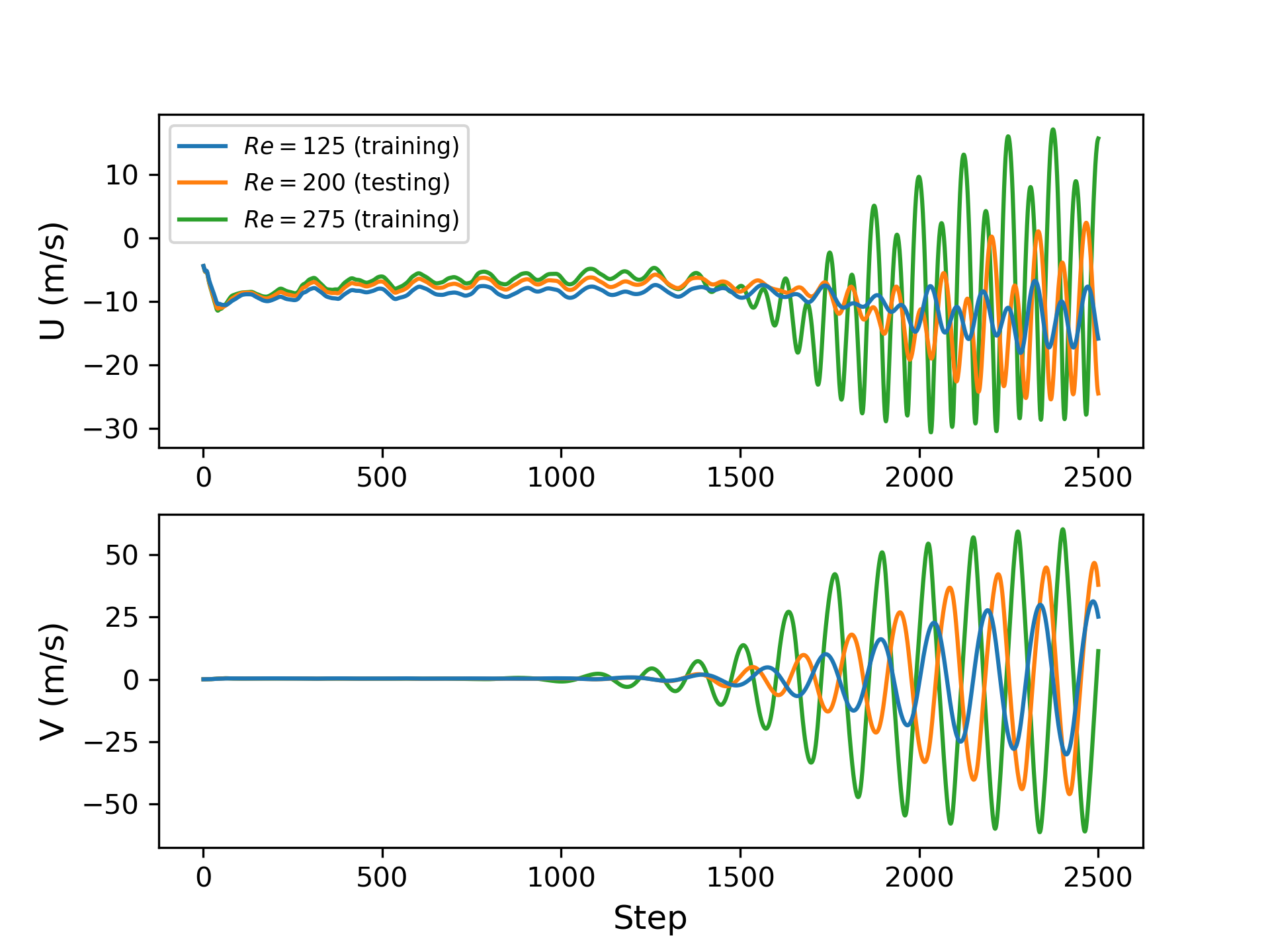
Figure 14: Transient flow over a cylinder: variable history at point monitor

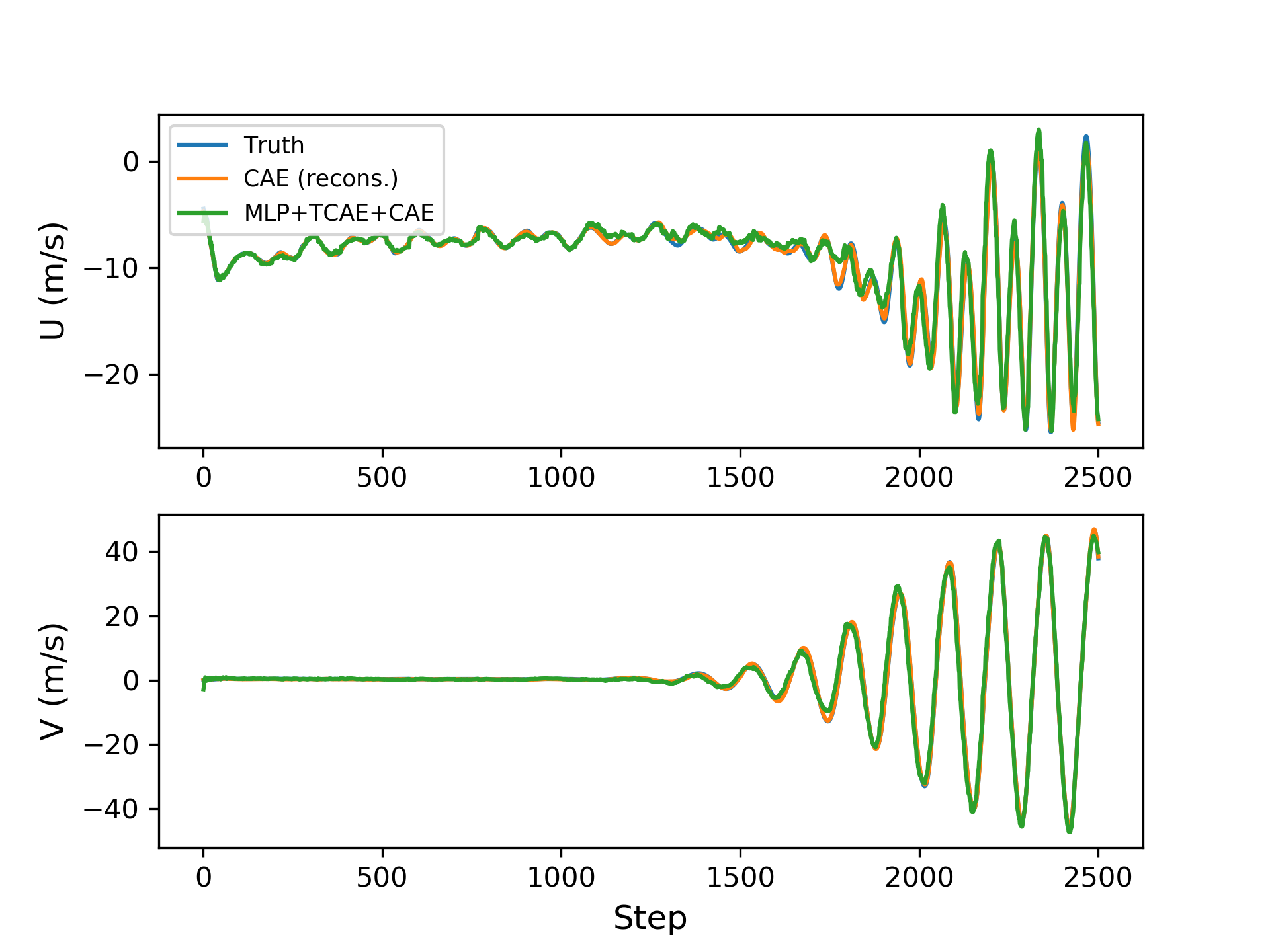
Figure 15: Transient flow over a cylinder new parameter prediction: reconstructed and predicted results at point monitor

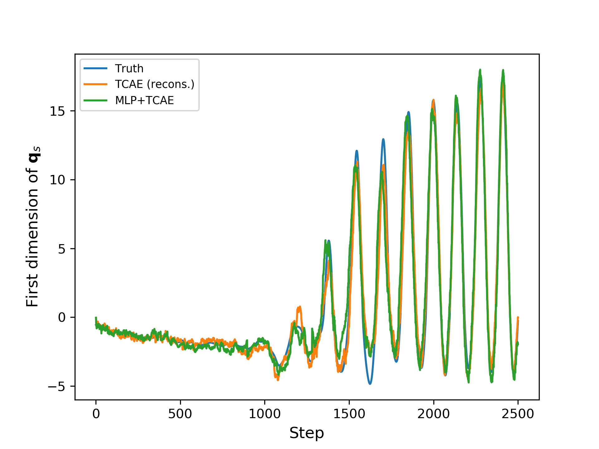
Figure 16: Transient flow over a cylinder new parameter prediction: first dimension of $\mathbf{q}_{s}$

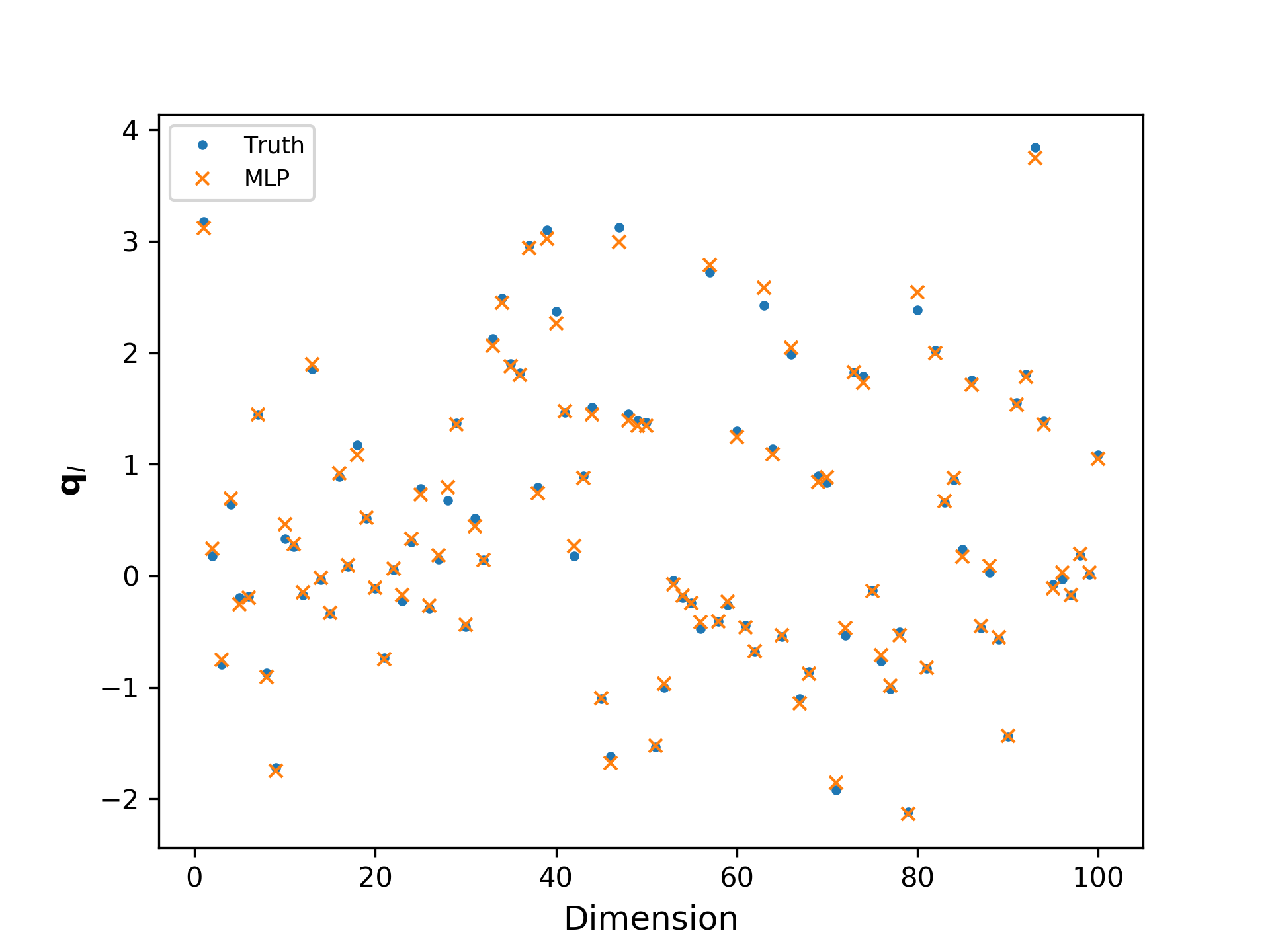
Figure 17: Transient flow over a cylinder new parameter prediction: $\mathbf{q}_{l}$

4.3.2 Combined prediction

In this task, prediction is performed beyond the training sequences (beyond 2500 frames) at the new parameter $Re=200$ for 500 future frames.

The CAE network is identical to that used in the new parameter prediction task. It is obvious in Fig. 15 that the unsteady flow field towards the end of the training sequence behaves significantly differently from the first half of the transition process, thus it is redundant to include the latter in the training of the TCN for future state prediction. Instead, only the last 500 frames in $\mathbf{Q}_{s}(Re_{\text{train}})$ are used in the training of $\mathcal{P}$. A look-back window of $n_{\tau}=150$ is used which corresponds to approximately one vortex shedding period for $Re=200$. $\mathcal{P}$ consists of a 5-layer strided TCN with $k=10$ and sequential dilation orders $d=1,2,4,8,16$ with 200 channels followed by a dense layer of output size $n_{s}=60$. The detailed architecture of $\mathcal{P}$ is given in Table 7d.

The predicted evolution of the first latent variable is shown in Fig. 19. The point monitor results of the decoded variables are shown in Fig. 19, and the contours for the last predicted step at $i=3000$ are provided in Fig. 20b. The RAE for the predicted velocity components is below 2%.

Table 8: Transient flow over a cylinder: errors for different stages of output

Stage		Truth	Output	RAE	MSE
Training ($Re=\{125,150,175,225,250,275\},$ frames 1 to 2500)		$\mathbf{q}\,(U/V)$	$\mathbf{\tilde{q}}\,(U/V)=\mathbf{\Psi}_{s}(\mathbf{\Phi}_{s}(\mathbf{q}))$	0.05%/0.09%	0.010/0.011
		$\mathbf{Q}_{s}=\mathbf{\Phi}_{s}(\mathbf{Q})$	$\tilde{\mathbf{Q}}_{s}=\mathbf{\Psi}_{l}(\mathbf{\Phi}_{l}(\mathbf{Q}_{s}))$	0.82%	0.06
		$\mathbf{q}_{l}=\mathbf{\Phi}_{(}\mathbf{Q}_{s})$	$\mathbf{q}_{l}^{*}=\mathcal{R}(Re)$	0.56%	$1.210-3$
Testing ($Re=200$)	Frames 1 to 2500	$\mathbf{q}\,(U/V)$	$\mathbf{\tilde{q}}\,(U/V)=\mathbf{\Psi}_{s}(\mathbf{\Phi}_{s}(\mathbf{q}))$	0.11%/0.19%	0.059/0.059
		$\mathbf{Q}_{s}=\mathbf{\Phi}_{s}(\mathbf{Q})$	$\tilde{\mathbf{Q}}_{s}=\mathbf{\Psi}_{l}(\mathbf{\Phi}_{l}(\mathbf{Q}_{s}))$	1.71%	0.31
		$\mathbf{q}_{l}=\mathbf{\Phi}_{(}\mathbf{Q}_{s})$	$\mathbf{q}_{l}^{*}=\mathcal{R}(Re)$	1.02%	$2.610-3$
		$\mathbf{Q}_{s}=\mathbf{\Phi}_{s}(\mathbf{Q})$	$\tilde{\mathbf{Q}}_{s}^{*}=\mathbf{\Psi}_{l}(\mathbf{q}_{l}^{*})$	1.99%	0.52
		$\mathbf{Q}\,(U/V)$	$\tilde{\mathbf{Q}}^{*}\,(U/V)=\mathbf{\Psi}_{s}(\tilde{\mathbf{Q}}_{s}^{*})$	0.68%/1.37%	2.37/7.02
	Frames 2501 to 3000	$\mathbf{q}_{s}=\mathbf{\Phi}_{s}(\mathbf{q})$	$\tilde{\mathbf{q}}_{s}=\mathcal{P}(\mathbf{Q}_{s})$	2.94%	0.80
		$\mathbf{q}\,(U/V)$	$\tilde{\mathbf{q}}^{*}\,(U/V)=\mathbf{\Psi}_{s}(\tilde{\mathbf{q}}_{s})$	1.18%/1.92%	3.72/8.34

The computing time by different parts of the framework in training and prediction for the combined prediction task is listed in Table 9. The total prediction time for 3000 frames for a new Reynolds number is less than 6.2 s. In comparison, the original CFD simulation is conducted with an in-house solver GEMS (General Equation and Mesh Solver) developed by Purdue University [76], which uses a implicit time marching method with 10 sub-iterations per time step. The simulation takes 15870.2 s on a 18-core Intel Xeon Gold 6154 CPU running at 3.70GHz. Thus, more than three orders of magnitude acceleration is achieved.

Table 9: Transient flow over a cylinder: computing time

Training
Component	CAE	TCAE	MLP	TCN	Total
Training epochs	200	1500	2000	300	-
Computing time (s)	8735	979	84	343	10141
Prediction
Component	$\mathbf{\Psi}_{s}$ (3000 frames)	$\mathbf{\Psi}_{l}$ (2500 frames)	MLP	TCN (500 frames)	Total (3000 frames)
Computing time (s)	5.46	0.13	0.011	0.57	6.171

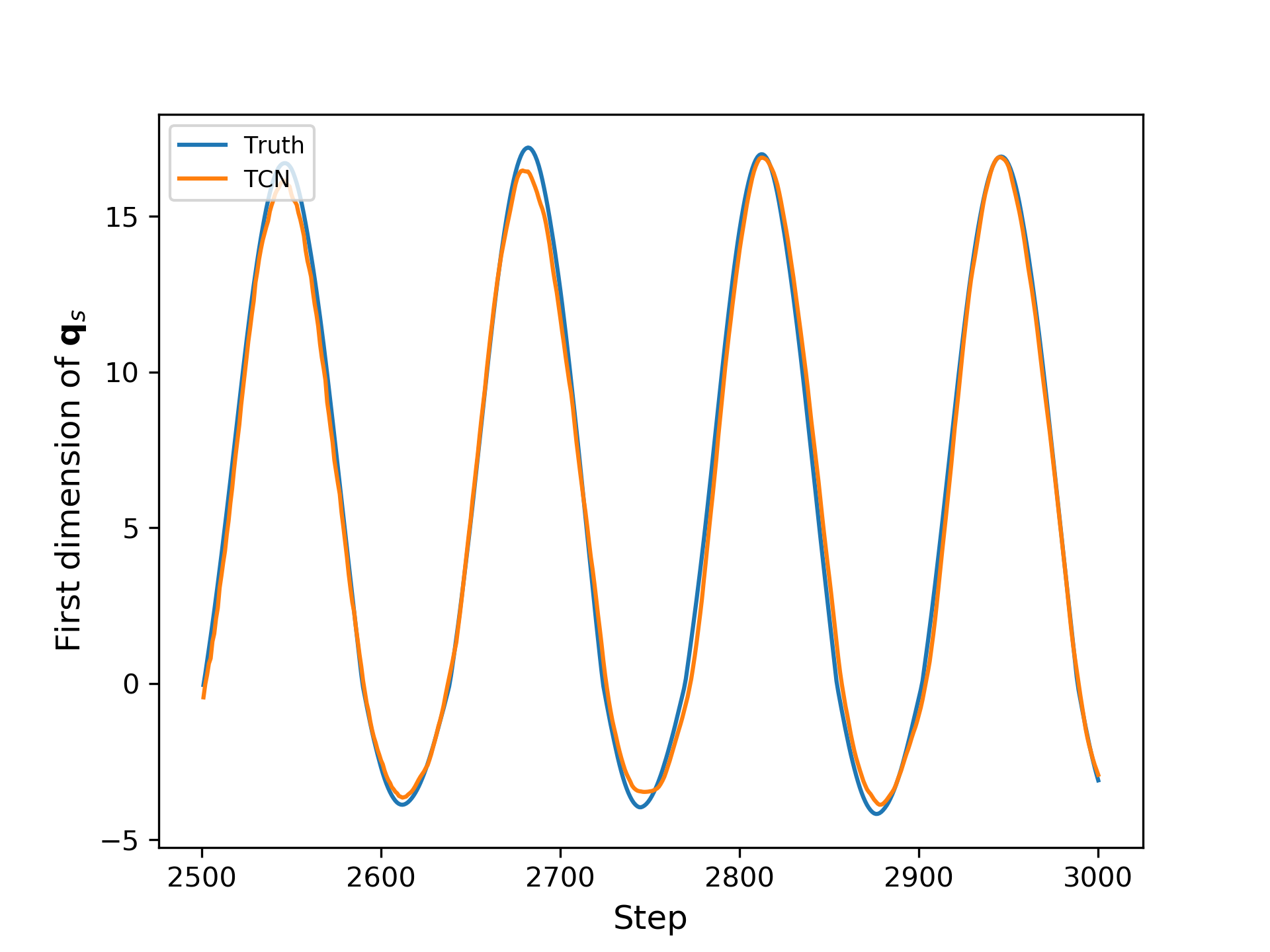
Figure 18: Transient flow over a cylinder combined prediction: first dimension of $\mathbf{q}_{s}$

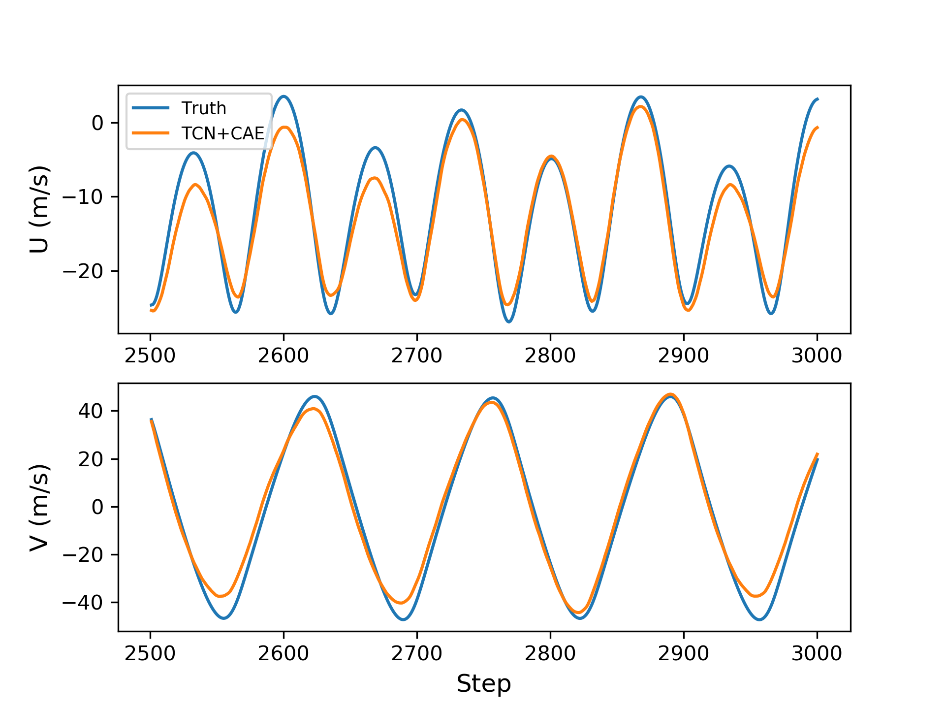
(a)

Figure 19: Transient flow over a cylinder combined prediction: predicted results at point monitor

(a) Truth

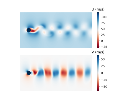
(b) Combined prediction

Figure 20: Transient flow over a cylinder combined prediction: flow field contours for $i=3000,Re=200$

4.4 Transient ship airwake

In this test, a new parameter prediction is performed on a three-dimensional flow behind a shipstructure. The inflow side-slip angle $\alpha$, i.e. the angle between inflow and ship cruising directions, is taken as the studied global parameter. Small variations in $\alpha$ introduce significant changes in the flow structures in the wake of the ship. The streamwise ($x$-direction), beamwise ($z$-direction) and vertical ($z$-direction) velocity components, $U,V,W$ are the variables of interest. The ship geometry is based on the Simple Frigate Shape Version 2 (SFS2) model [77], which features a double-level ship structure that results in significant flow separation over the deck. More details about the model can be found in Ref. [77]

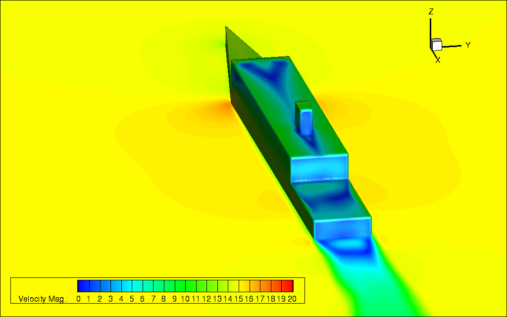
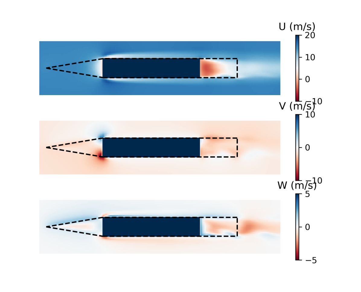
(a) $\alpha=0\degree$

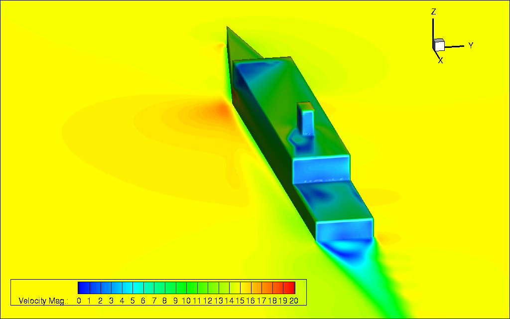
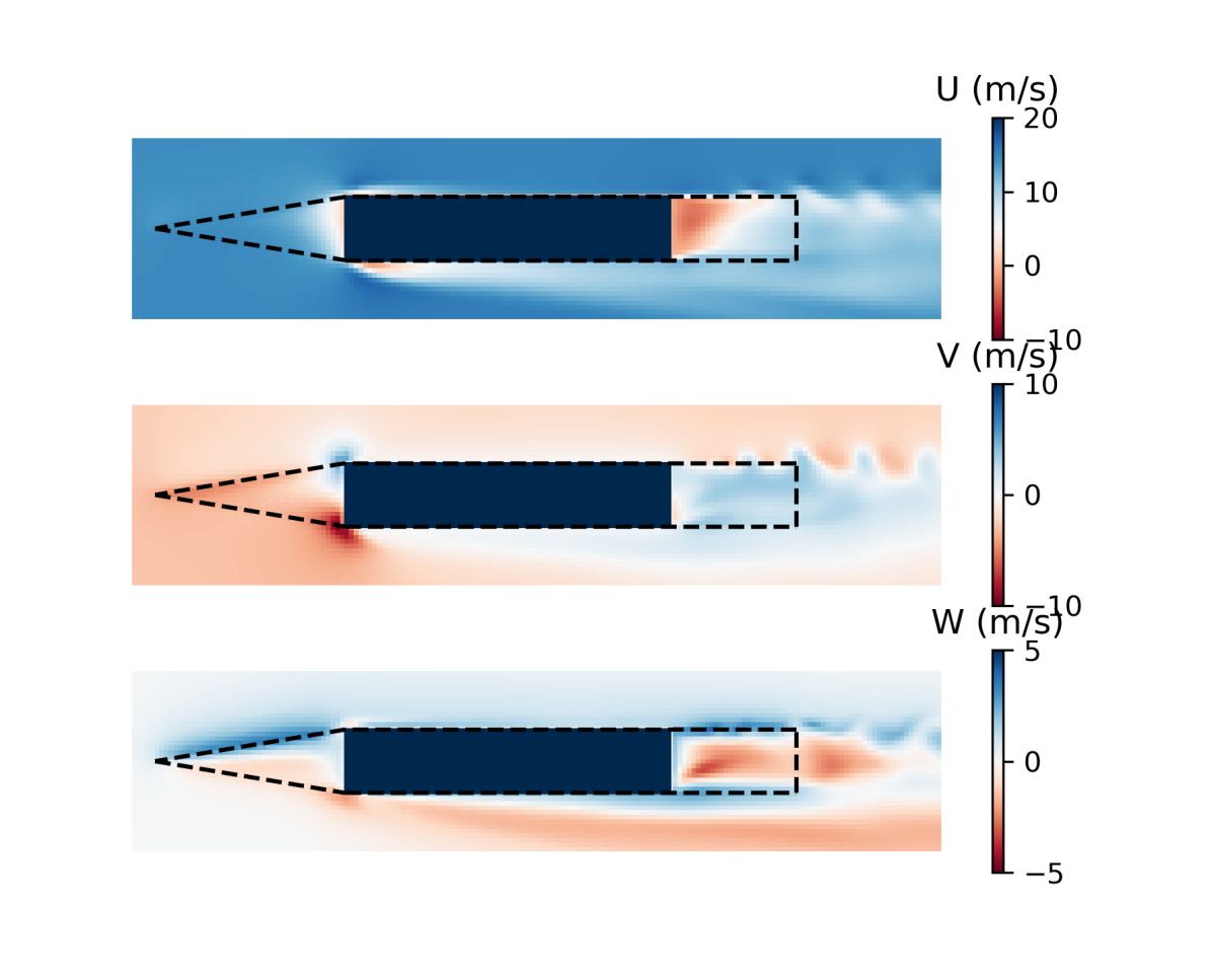
(b) $\alpha=10\degree$

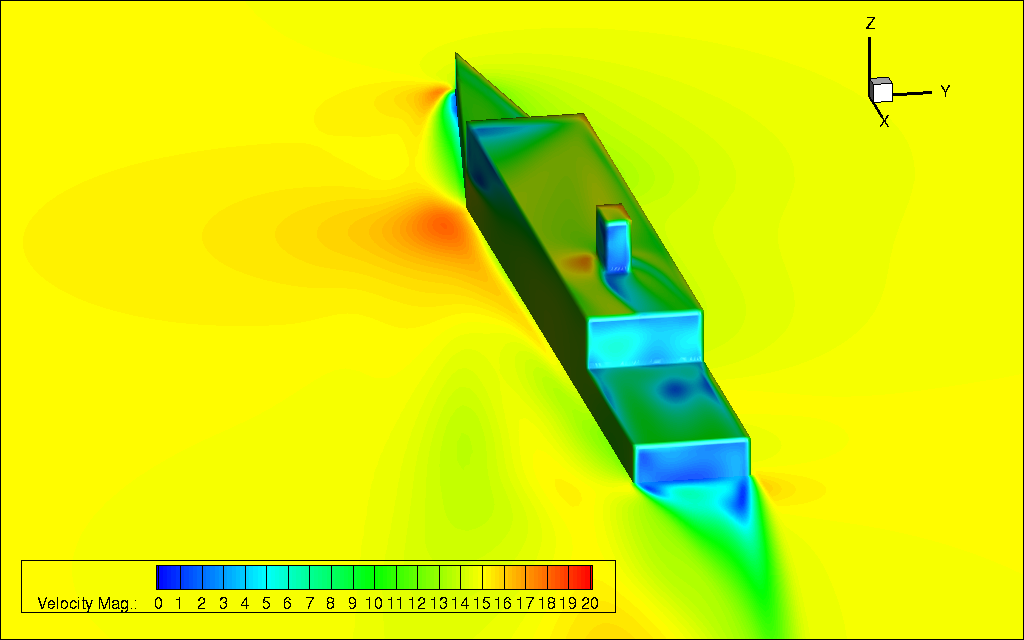
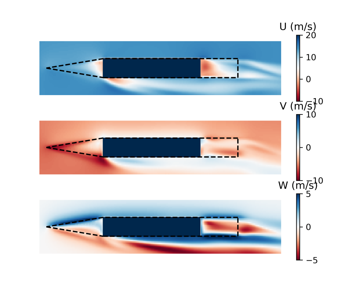
(c) $\alpha=20\degree$

Figure 21: Transient ship airwake: sample frame of settled unsteady patterns. Top: velocity magnitudes; bottom: velocity components.

The ground truth flow field is computed using unsteady Reynolds Averaged Navier-Stokes equations with the $k-\omega$ turbulence model [78]. 4 sets of training data corresponding to the new inflow angles $\alpha=\{5\degree,10\degree,15\degree,20\degree\}$ are provided, and prediction is performed for $\alpha=12.5\degree$. In all the cases, the ship is originally cruising in a headwind condition, i.e. $\alpha=0{\color[rgb]{1,0,0}\degree}$, then the side-slip angle is impulsively changed, causing the flow to transition to a different unsteady state. The velocity magnitude for a sample frame of the settled unsteady pattern for three different $\alpha$ and the corresponding velocity components on a x-y plane 5 meters above the sea level (slightly above the deck) are shown in Fig. 21.

Predictions are focused on a 3D near-field region surrounding the ship of dimensions length $\times$ width $\times$ height = 175 m $\times$ 39 m $\times$ 23 m. The size of the interpolated Cartesian grid is $n_{x}\times n_{y}\times n_{z}=176\times 40\times 24$. Each data set includes 400 frames corresponding to 40 s of physical time. Errors for different stages of output are summarized in Table 11.

Table 10: Transient ship airwake: network architectures

$\mathbf{\Phi}_{s}$
Layer	Input	Conv-pool	Conv-pool	Conv-pool	Conv-pool	Flatten	Dense (Output)
Output shape	$400\times 40\times 24\times 3$	$200\times 20\times 12\times 64$	$100\times 10\times 6\times 128$	$50\times 5\times 6\times 256$	$25\times 5\times 6\times 256$	192000	20
$\mathbf{\Psi}_{s}$
Layer	Input	Dense	Reshape	Conv-trans	Conv-trans	Conv-trans	Conv-trans (Output)
Output shape	20	192000	$25\times 5\times 6\times 256$	$50\times 5\times 6\times 256$	$100\times 10\times 6\times 128$	$200\times 20\times 12\times 64$	$400\times 40\times 24\times 3$

(a) CAE

$\mathbf{\Phi}_{l}$
Layer	Input		9-layer TCN block	Dense (Output)
Output shape	$20\times 400$		400	20
$\mathbf{\Psi}_{l}$
Layer	Input	Dense	Repeat vector	9-layer TCN block (Output)
Output shape	20	400	$400\times 400$	$20\times 400$

(b) TCAE

Layer	Input	Dense	Dense	Dense (Output)
Output shape	1	16	50	20

(c) MLP

The top level CAE contains 4 Conv-pool blocks and 1 dense layer in the encoder with a encoded latent dimension of $n_{s}=20$. The detailed CAE architecture is provided in Table 10a. The CAE reconstruction $\mathbf{\tilde{q}}=\mathbf{\Psi}_{s}(\mathbf{\Phi}_{s}(\mathbf{q}))$ shows a RAE around 0.1%. A comparison between the original and reconstructed flow field for $\alpha=12.5\degree$ at the 400-th frame is provided in Fig. 22a and 22b. The monitored history for the reconstructed variables at a point 1 meter above the center of the deck of the SFS2 model is compared with the ground truth in Fig. 24.

The TCN block in $\mathbf{\Phi}_{l}$ of the TCAE contains 9 dilated convolution layers, with a uniform kernel size $k=10$ and sequential dilation orders $d=1,2,2^{2},\dots,2^{7},2^{8}$. A dense layer is appended after the TCN block, and the encoded latent dimension is $n_{l}=20$. The reconstructed sequence $\tilde{\mathbf{Q}}_{s}=\mathbf{\Psi}_{l}(\mathbf{\Phi}_{l}(\mathbf{Q}_{s}))$ shows a RAE of 4.47% in the testing stage.

A MLP of 3 dense layers is used for the third level, the details of which is given in Table 10c. The accuracy of the MLP prediction is assessed in Fig. 24. The RAE for final predicted velocity components $\mathbf{Q}^{*}=\mathbf{\Psi}_{s}(\mathbf{\Psi}_{l}(\mathbf{q}_{l}^{*}))$ are below 0.9%. The last frame of the solution is shown in Fig. 22c. The predictions are seen to be accurate, despite significant variations in unsteady patterns between the testing condition and the training ones represented in Fig. 22. The point monitor history is shown in Fig. 24 where the trend of dynamics is captured closely.

The computing time by different parts of the framework in training and prediction for the combined prediction task is listed in Table 12. The total prediction time for 400 frames of the 3D unsteady flow field is about 6.6 s. In comparison, the original CFD simulation takes 4011.5 s using a commercial parallel solver Ansys Fluent on a six-core Intel Xeon E5-1650 CPU running at 3.60GHz. Thus, $>600\times$ reduction in computational cost is achieved.

Table 11: Transient ship airwake: errors for different stages of output

Stage	Truth	Output	RAE	MSE
Training ($\alpha=\{5\degree,10\degree,15\degree,20\degree\}$)	$\mathbf{q}\,(U/V/W)$	$\mathbf{\tilde{q}}\,(U/V/W)=\mathbf{\Psi}_{s}(\mathbf{\Phi}_{s}(\mathbf{q}))$	0.12%/0.09%/0.08%	$2.010-3$/$5.910-4$/$2.510-4$
	$\mathbf{Q}_{s}=\mathbf{\Phi}_{s}(\mathbf{Q})$	$\tilde{\mathbf{Q}}_{s}=\mathbf{\Psi}_{l}(\mathbf{\Phi}_{l}(\mathbf{Q}_{s}))$	0.63%	2.18
	$\mathbf{q}_{l}=\mathbf{\Phi}_{(}\mathbf{Q}_{s})$	$\mathbf{q}_{l}^{*}=\mathcal{R}(\alpha)$	0.60%	$1.610-3$
Testing ($\alpha=12.5\degree$)	$\mathbf{q}\,(U/V/W)$	$\mathbf{\tilde{q}}\,(U/V/W)=\mathbf{\Psi}_{s}(\mathbf{\Phi}_{s}(\mathbf{q}))$	0.30%/0.38%/0.29%	$1.410-2$/$5.810-3$/$2.710-3$
	$\mathbf{Q}_{s}=\mathbf{\Phi}_{s}(\mathbf{Q})$	$\tilde{\mathbf{Q}}_{s}=\mathbf{\Psi}_{l}(\mathbf{\Phi}_{l}(\mathbf{Q}_{s}))$	4.47%	65.54
	$\mathbf{q}_{l}=\mathbf{\Phi}_{(}\mathbf{Q}_{s})$	$\mathbf{q}_{l}^{*}=\mathcal{R}(\alpha)$	0.85%	$2.610-3$
	$\mathbf{Q}_{s}=\mathbf{\Phi}_{s}(\mathbf{Q})$	$\tilde{\mathbf{Q}}_{s}^{*}=\mathbf{\Psi}_{l}(\mathbf{q}_{l}^{*})$	4.44%	65.82
	$\mathbf{Q}\,(U/V/W)$	$\tilde{\mathbf{Q}}^{*}\,(U/V/W)=\mathbf{\Psi}_{s}(\tilde{\mathbf{Q}}_{s}^{*})$	0.51%/0.89%/0.62%	0.045/0.049/0.014

Table 12: Transient ship airwake: computing time

Training
Component	CAE	TCAE	MLP	Total
Training epochs	500	500	2500	-
Computing time (s)	12705	213	27	12945
Prediction
Component	$\mathbf{\Psi}_{s}$ (400 frames)	$\mathbf{\Psi}_{l}$ (400 frames)	MLP	Total (400 frames)
Computing time (s)	5.71	0.89	0.005	6.605

(a) Truth, $\mathbf{q}$

(b) CAE reconstruction

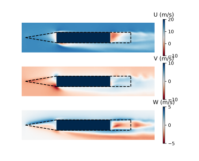
(c) MLP+TCAE+CAE

Figure 22: Transient ship airwake: x-y plane velocity components for $i=400,\alpha=12.5\degree$

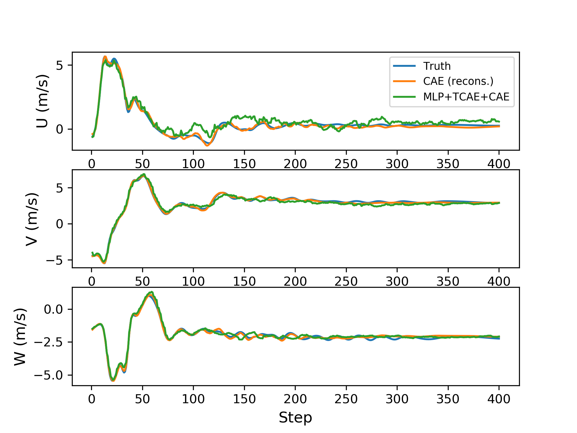
Figure 23: Transient ship airwake: reconstructed and predicted results at point monitor

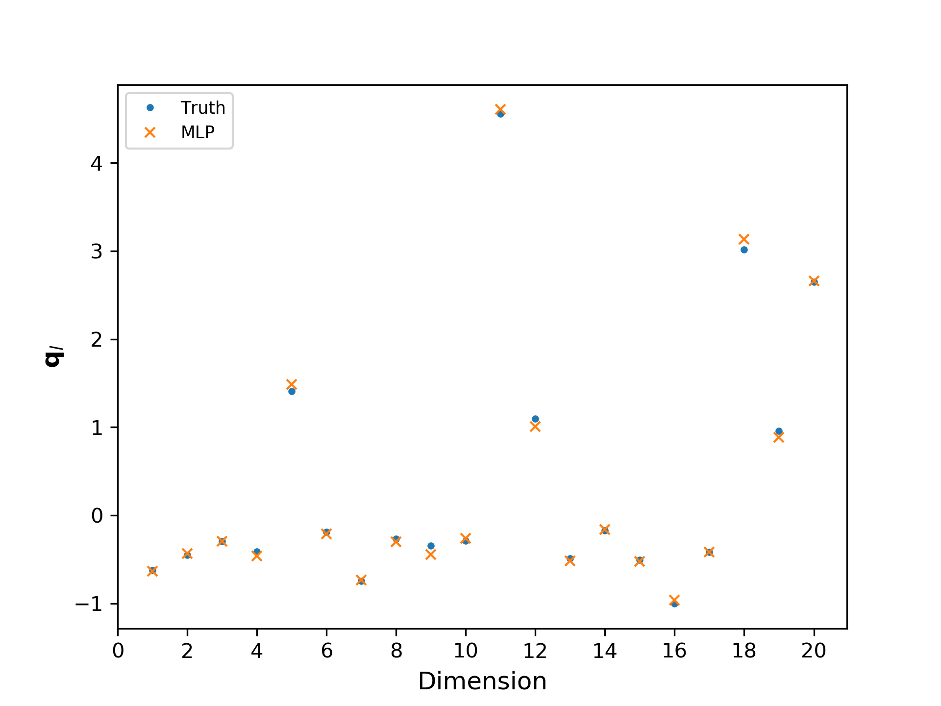
Figure 24: Transient ship airwake: $\mathbf{q}_{l}$

5 Perspectives

Overall, the results suggest that given adequate data and careful training, effective data-driven models can be constructed using multi-level neural networks. A pertinent question - and one of the original motivations for the authors to pursue this research - is how the present approach compares to classical and emerging intrusive projection-based model reduction techniques. The input data for this framework is similar to that used in projection-based model reduction techniques. The present approach is however completely non-intrusive in the sense that the governing equations and partial differential equation solvers and codes therein are not used. These techniques, therefore, fall in the class of non-intrusive operator inference methods such as those presented in Refs. [22, 41, 48], which leverage POD rather than neural networks to identify the first level (spatially encoded) of latent variables $\mathbf{Q}_{s}$.

The non-intrusive nature of the framework greatly simplifies the development process and time. Further, the proposed techniques are orders of magnitude less expensive in execution time than standard projection-based models. Indeed, model training was performed in a few GPU hours, and all the predictions were executed in a few seconds. The availability of efficient open-source libraries for deep learning is another advantage of this approach.

To the contrary, it can be argued that the use of governing equations such as in projection-based reduced order models can reduce the amount of data required, and present more opportunities to enforce physical constraints. Although the authors have not seen clear evidence of advantages of intrusive methods based on a few experiments, this aspect nevertheless requires disciplined evaluations on a series of benchmark problems. It has to be recognized, however, that intrusive ROMs are prone to and highly sensitive to numerical oscillations and require special treatment [76, 79] to ensure robustness in complex flows, whereas non-intrusive ROMs are much more flexible.

Lee and Carlberg [28] use autoencoders to identify the latent space, and solve the governing equations on this manifold using Galerkin and Petrov-Galerkin approaches, instead of TCN-based time steppers as in the present work. Ref. [28] is an intrusive approach, and thus requires further development of sparse sampling techniques to be more efficient than the full order model it approximates. Nevertheless, such techniques possess the added appeal of guarantees on consistency and optimality, and would be a natural candidate to evaluate the pro and cons of the present approach.

A general critique on neural network-based approaches is that they require “more data” compared to linear, and more structured compression techniques. Expressivity and generalization has to be balanced with the cost of obtaining data. Bayesian approaches can be used to construct operators and to optimally design data-generating experiments. Data requirements can also be reduced by including the governing equations in the loss function [80]. Moving beyond the reputation of neural networks being “black boxes,” there are prospects to enforce additional structure. For instance, Ref. [81] imposes structured embedding with guarantees on stability. Transformation of the state variables either by hand [82] or using learning algorithms [83, 81] may also be leveraged.

Finally, it should be recognized that the convolution operations pursued in this work are defined on Cartesian grids. Replacing the Euclidean convolution operations by graph convolutions [84] would enable application to predictions over generalized unstructured meshes.

6 Summary

A multi-level deep learning approach is proposed for the direct prediction of spatio-temporal dynamics. The framework is designed to address parametric and future state prediction. The data is processed as a uniformly sampled sequence of time snapshots of the spatial field. A convolutional autoencoder (CAE) serves as the top level, encoding each time snapshot into a set of latent variables. Temporal convolutional networks (TCNs) serve as the second level to process the output sequence. The TCN is a unique feature of the framework. Unlike in standard convolutions in which the receptive field growths linearly with the number of layers and the kernel size, dilated convolutions in the TCN allow for exponential growth of the reception field, leading to more efficient processing of long temporal sequences. For parametric predictions, a TCAE is used to further encode the sequence of spatially encoded variables $\mathbf{Q}_{s}$ along the temporal dimension into a second set of latent variables $\mathbf{q}_{l}$, which is the encoded spatio-temporal evolution. A multi-layer perceptron (MLP) is used as the third level to learn the mapping between $\mathbf{q}_{l}$ and the global parameters $\mu$. For future state predictions, the second level iteratively uses a TCN to predict $\mathbf{Q}_{s}(\mu)$. In either type of task, outputs at the bottom level are decoded to obtain the predictions for high-dimensional spatio-temporal dynamics for desired conditions.

Numerical tests in a one-dimensional compressible flow problem demonstrate the capability of the framework to accurately predict the motion of discontinuities and waves beyond the training period. It is notable that this capability is impossible in linear basis techniques (such as POD), even when the governing equations are used intrusively as in projection-based ROMs. Evaluations on transient two and three dimensional flows with coherent structures demonstrates parametric and future state prediction capabilities, even when there are significant changes in the flow topology for the prediction configuration. The CAE is also shown to perform significantly better than POD to extract the latent variables, especially when future state prediction is involved. Sensitivity of the results to the amount of input data, the size of the latent space and other modeling choices is explored.

As such, we do not recommend our approach as a replacement to traditional model reduction methods, or that CAEs should necessarily replace POD for all classes of problems. Parsimoniously parameterized models informed by PDE-based physics constraints have formed the basis of scientific modeling, and will continue to be useful. However, we find the results compelling enough to be worthy of serious debate, especially when adequate data is available.

7 Acknowledgments

The authors acknowledge support from the Air Force under the Center of Excellence grant FA9550-17-1-0195, titled Multi-Fidelity Modeling of Rocket Combustor Dynamics (Program Managers: Dr. Mitat Birken and Dr. Fariba Fahroo), and the Office of Naval Research grant N00014-16-1-2728 titled A Surrogate Based Framework for Helicopter/Ship Dynamic Interface, (Program manager: Dr. Brian Holm-Hansen).

References

Appendix A Replacement of CAE with POD

In this section, the top level CAE is replaced with POD to provide a direct performance comparison between linear and nonlinear latent spaces. The POD basis is computed in a coupled manner, i.e. all the variables are flattened into a vector $\mathbf{s}\in\mathds{R}^{n}$ for each frame of data, and these vectors are combined as columns in the snapshot matrix $\mathbf{S}\in\mathds{R}^{n\times n_{t}}$. Before the flattening and collection of snapshots, the same standard deviation scaling as for CAE is applied to the variables. In other words, $\mathbf{S}$ is simply a flattened version of the input $\mathbf{Q}$ of CAE. For clarity, we will use $\mathbf{q}$ and $\mathbf{Q}$ to refer to a single frame and the entire sequence of inputs for both POD and CAE. SVD is performed on the snapshot matrix to obtain the POD basis. Each mode of the basis contains information about all variables, enabling a direct comparison with the CAE.

Assuming $n_{k}$ to be the designed number of modes, POD basis $\mathbf{V}\in\mathds{R}^{n\times n_{k}}$ is constructed from the first $n_{k}$ left-singular vectors from the SVD. The corresponding spatially compressed variable is

$$\mathbf{q}_{s}=\mathbf{V}^{T}\mathbf{q}.$$ (26)

For a given $\mathbf{q}_{s}$, the full order solution is then approximated by

$$\mathbf{\tilde{q}}=\mathbf{V}\mathbf{q}_{s}.$$ (27)

We will refer to the compression and reconstruction processes as encoding and decoding, respectively.

A.1 Discontinuous compressible flow

The training data for the shock tube only contains 35 time steps, and thus the total number of effective POD modes is limited to $n_{k}=35$. Since all POD modes are used, an exact reconstruction of the training data is achieved. However, in prediction, the waves propagate outside the region in which training features were present, and thus the global basis fails immediately. The reconstruction results for $t=0.25$ s are shown in Fig. 25 along with the truth and the ending frame in the training data, which corresponds to $t=0.1$ s.

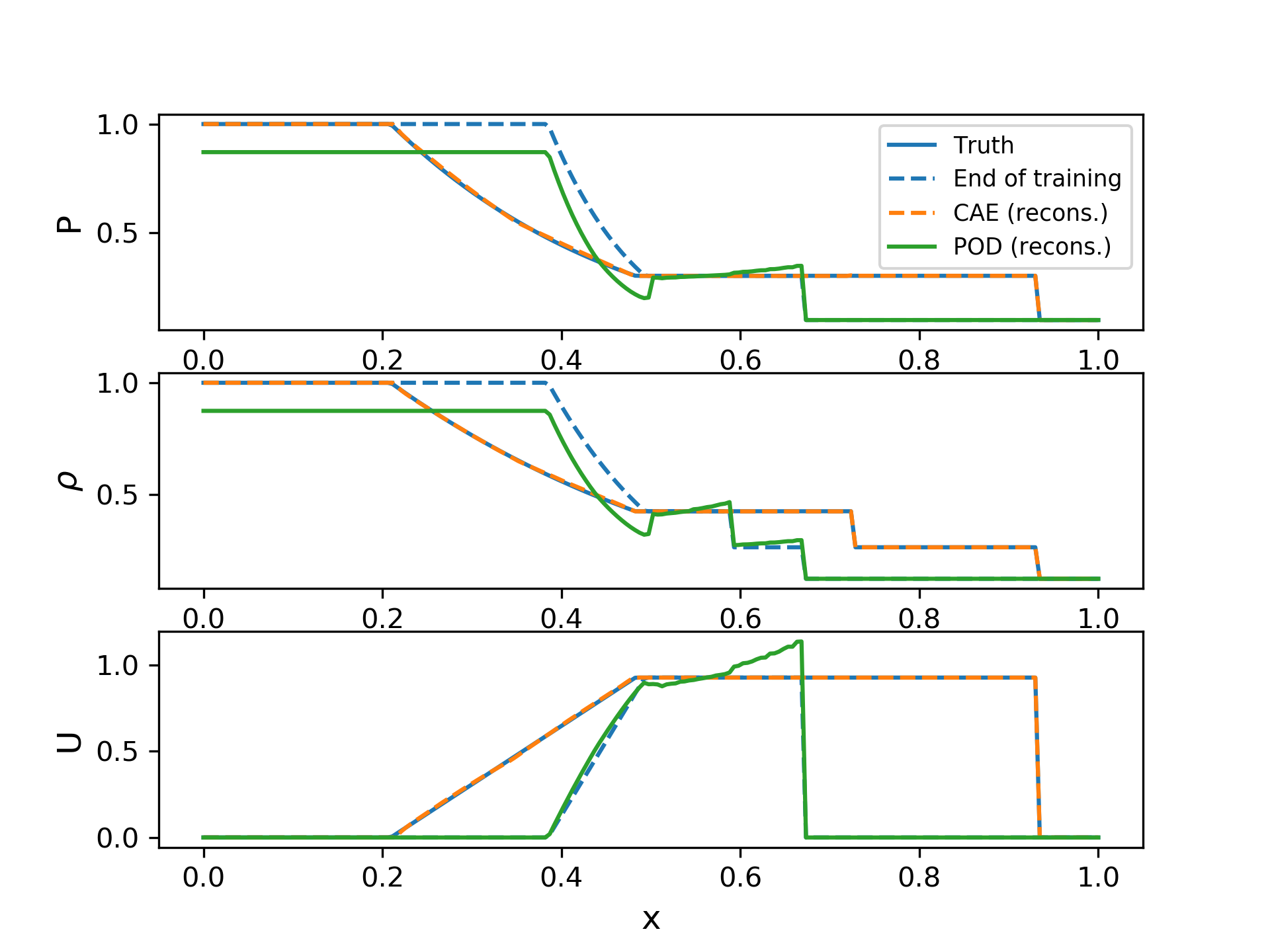
(a)

Figure 25: Discontinuous compressible flow: POD reconstructed variables for $t=0.25$ s

A.2 Transient flow over a cylinder

In this test, the number of POD modes is set to be the same as the latent dimension of the CAE, i.e. $n_{k}=n_{s}=60$. Other than replacing the CAE with POD, the neural network settings remain identical to the CAE-based combined prediction in Sec. 4.3. The same training and predictions as in Sec 4.3 are repeated and the RAE for different stages is summarized in Table 13.

Table 13: Transient flow over a cylinder: RAE for frameworks with CAE- and POD-based spatial compression

Frame	Variable	CAE-based		POD-based
		Train	Test	Train	Test
1 to 2500	CAE/POD reconstruction, $\mathbf{Q}\,(U/V)$	0.05%/0.09%	0.11%/0.19%	0.39%/0.41%	0.38%/0.45%
	TCAE reconstruction, $\mathbf{Q}_{s}$	0.75%	1.71%	0.66%	1.62%
	MLP prediction, $\mathbf{q}_{l}$	0.56%	1.02%	0.8%	2.2%
	Framework prediction, $\mathbf{Q}\,(U/V)$	-	0.68%/1.37%	-	1.01%/1.97%
2501 to 3000	CAE/POD reconstruction, $\mathbf{Q}\,(U/V)$	-	0.19%/0.41%	-	0.47%/0.62%
	TCN prediction, $\mathbf{Q}_{s}$	0.21%	2.94%	0.15%	2.20%
	Framework prediction, $\mathbf{Q}\,(U/V)$	-	1.18%/1.92%	-	1.69%/4.14%

It can be seen that the error for spatial reconstruction using POD is significantly larger than that of the CAE in both training and testing. This is visualized by the dashed lines in Fig. 27.

The performance of the time-series processing of the encoded sequence $\mathbf{Q}_{s}$ using TCAE or TCN is independent of the spatial encoding. Indeed, from the plot of the first dimension of $\mathbf{q}_{s}$ in Fig. 27, it can be seen that curve is smoother than the point monitor result for the physical variables in Fig. 27 or the latent variable encoded using CAE in Fig. 17, thus reducing the error in the TCAE and TCN predictions for the latent variable slightly.

The final prediction accuracy is largely limited by the POD performance when the predicted encoded variables are decoded. The final POD-based prediction result fails to represent the dynamics, as is clear from the point monitor result in Fig. 27. It is noted that the relative error listed in Table 13 is noticeably larger than that for the CAE-based result, though it is not visible in the figure. This is because that the error is averaged over the spatio-temporal span including a large range of low-amplitude unsteady or even steady data. To provide a more direct comparison of the prediction results, the flow field contours for the 1650th frame, where a large deviation from the truth is observed in the POD result, and the last, i.e. the 3000th frame, where the accumulative error in the future state prediction is maximized, are shoown in Fig. 28. It can be seen that the POD-based framework fails to capture certain details of the vortex structures whereas the CAE-based prediction is significantly closer to the truth.

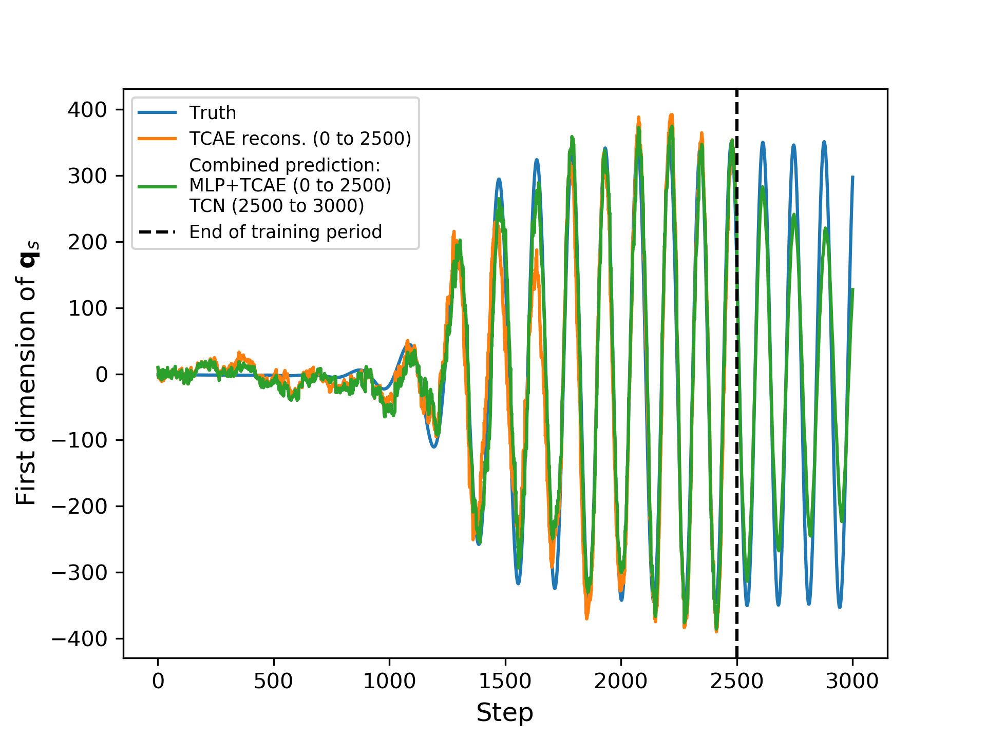
Figure 26: Transient flow over a cylinder: first dimension of $\mathbf{q}_{s}$ in POD-based framework

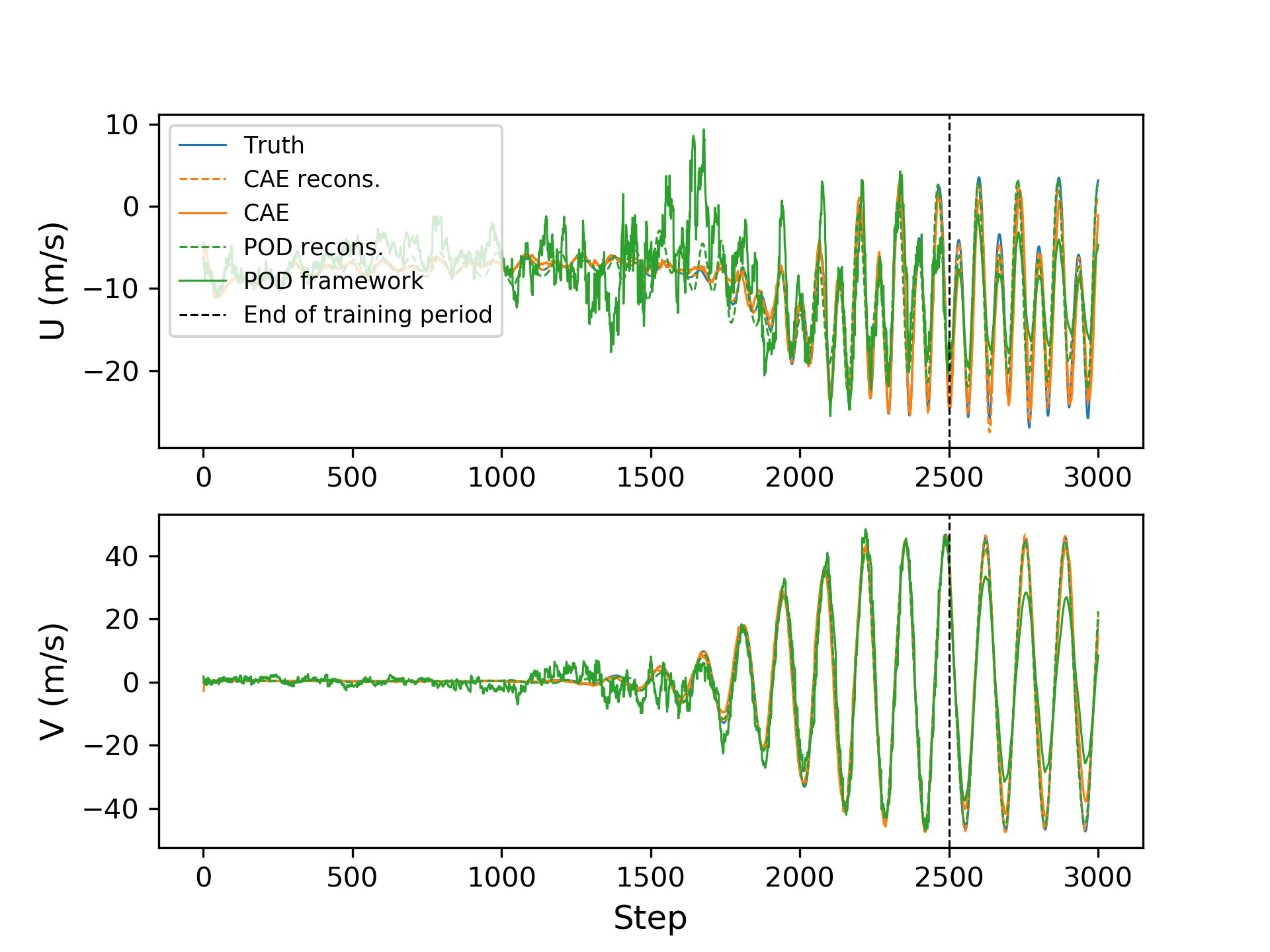
Figure 27: Transient flow over a cylinder: point monitor results for CAE- and POD-based frameworks

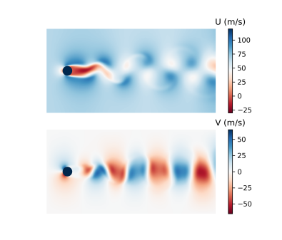
(a) Truth, $i=1650$

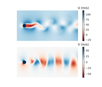
(b) CAE prediction, $i=1650$

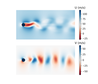
(c) POD prediction, $i=1650$

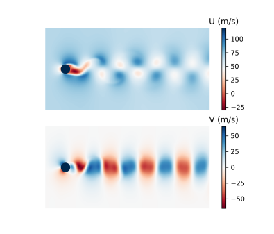
(d) Truth, $i=3000$

(e) CAE prediction, $i=3000$

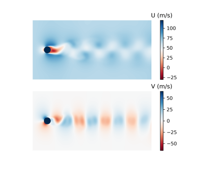
(f) POD prediction, $i=3000$

Figure 28: Transient flow over a cylinder: flow contours from CAE- and POD-based frameworks

A.3 Transient ship airwake

As in the previous example, the encoded dimensions are set to be the same for POD and CAE, i.e. $n_{k}=n_{s}=20$. The same second and third level network architectures are used as in Sec. 4.4. The RAE for different stages is summarized in Table 14.

Table 14: Transient ship airwake: RAE for frameworks with CAE- and POD-based spatial compression

Variable	CAE-based		POD-based
	Train	Test	Train	Test
CAE/POD reconstruction, $\mathbf{Q}\,(U/V/W)$	0.12%/0.09%/0.08%	0.30%/0.38%/0.29%	0.34%/0.37%/0.29%	0.42%/0.44%/0.41%
First 100 frames of reconstruction	-	2.28%/1.47%/1.18%	-	7.77%/6.20%/7.13%
TCAE reconstruction, $\mathbf{Q}_{s}$	0.63%	4.47%	0.20%	1.91%
MLP prediction, $\mathbf{q}_{l}$	0.60%	0.85%	0.96%	6.23%
Framework prediction, $\mathbf{Q}\,(U/V/W)$	-	0.51%/0.89%/0.62%	-	0.61%/0.91%/0.70%
First 100 frames of prediction	-	4.52%/3.94%/2.74%	-	9.02%/6.49%/7.91%

A increase in the reconstruction error is observed especially in the testing stage. The same point monitor as in Sec. 4.4 is used and the result is shown in Fig. 29. It can be seen that the POD result largely deviates from the truth especially in the first 100 frames where transition from initial towards the new side-slip angle imposes a strong influence on the area over the deck. Error values for this period are listed in addition to those for the full sequence in Table 14, in order to better illustrate the discrepancy. The gap in performance is clearly visualized in the flow contours for $i=10$ in Fig. 30, where the POD-based prediction shows a blurred and shifted airwake whereas the CAE-based prediction appears to be almost visually identical to the truth. It should be noted that in Fig. 29 final POD-based framework prediction follows the POD reconstructed variables tightly, which illustrates reliable performance of the rest of the framework.

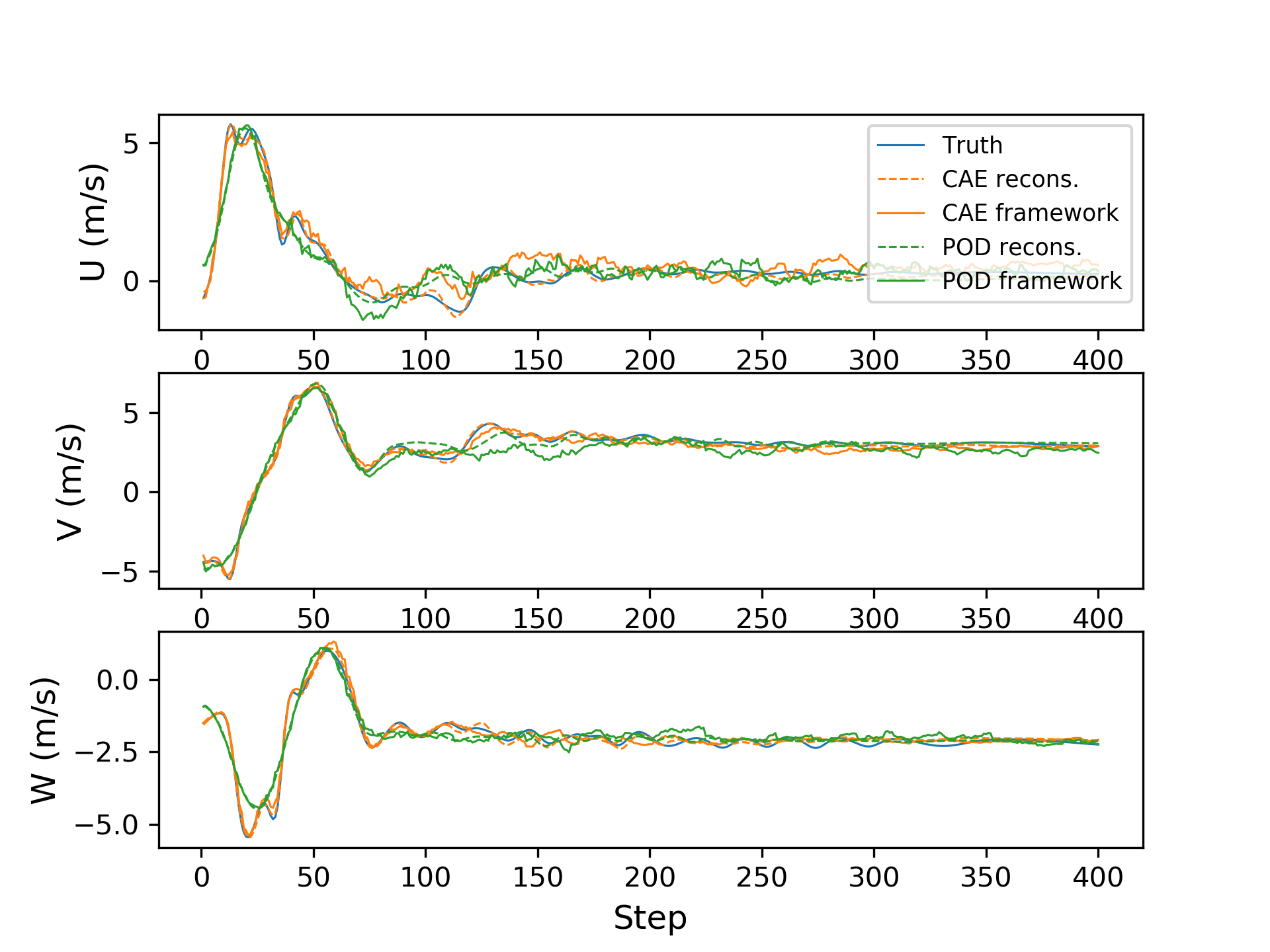
(a)

Figure 29: Transient ship airwake: point monitor results for CAE- and POD-based frameworks

(a) Truth

(b) CAE prediction

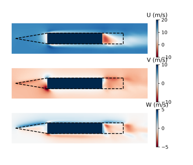
(c) POD prediction

Figure 30: Transient ship airwake: flow contours from CAE- and POD-based frameworks for $i=10$

Appendix B Latent dimension sensitivity study

Besides the nonlinearity, an important difference between the autoencoder and POD-based model reduction methods is that the latent dimension needs to be pre-determined in the design of the network structure before the training process. On the other hand, the SVD provides a full set of singular vectors, which can be truncated based on a priori error estimates. As a consequence, the sensitivity of the network performance w.r.t. the latent dimensions in the autoencoders becomes an important feature, and is assessed for the cylinder and ship airwake cases. The shock tube is not considered as compression is only performed on the number of variables.

B.1 Transient flow over a cylinder

The influence of $n_{s}$ on the CAE encoding-decoding accuracy is shown in Fig. 32. It can be seen that both training and testing errors experience a sharp drop for $n_{s}\leq 30$, following which the slope starts to flatten and the decay saturates for $n_{s}\geq 60$. For the TCAE result in Fig. 32, the decay in training error is almost negligible, yet the testing error drops rapidly for $n_{l}\leq 80$.

Due to the rapid decay in leading modes in both levels of autoencoders, the spatio-temporal sequence can be represented using a significantly reduced set of latent variables.

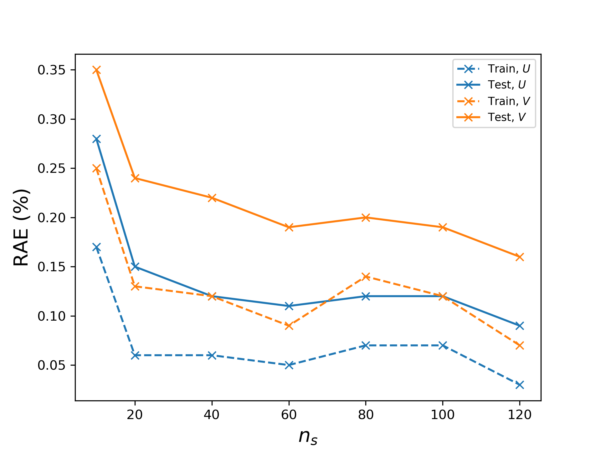
Figure 31: Transient flow over a cylinder: CAE RAE vs $n_{s}$

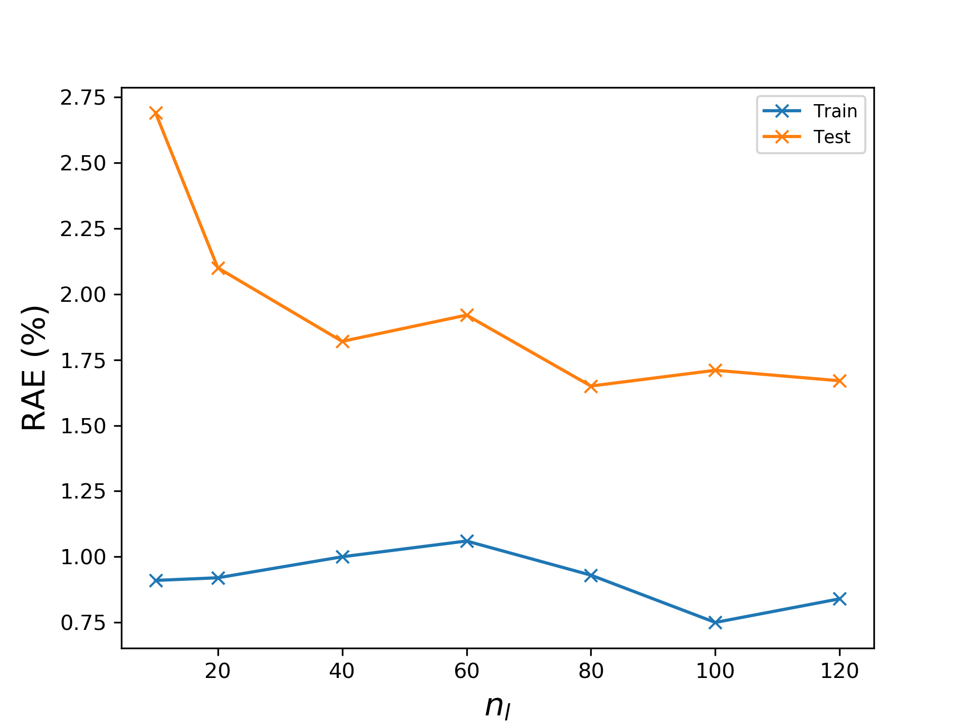
Figure 32: Transient flow over a cylinder: TCAE RAE vs $n_{l}$

B.2 Transient ship airwake

Compared to the previous case, the CAE testing error saturates at a few modes. This is a consequence of the fact that when the inflow side-slip angle changes, the similarity between the training and testing data is very limited in both large and small scales physics. Thus, including extensive latent dimensions does not reduce the testing error efficiently. Due to the same reason, the decay in the TCAE error is also slow. Nevertheless, the testing RAE is below 0.5% in the CAE and 5% in the TCAE, providing a highly efficient model reduction as shown in Sec. 4.4.

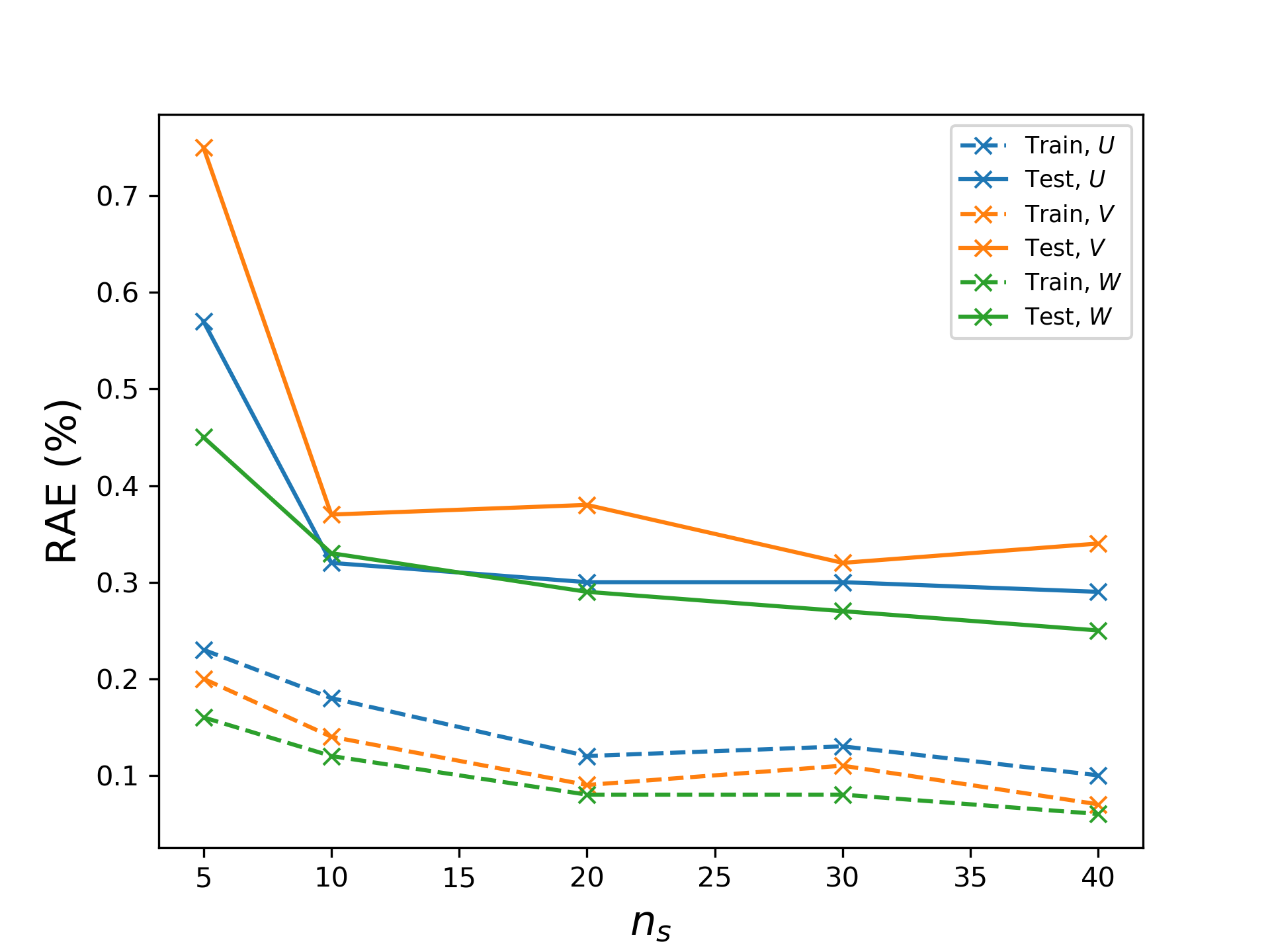
Figure 33: Transient ship airwake: CAE RAE vs $n_{s}$

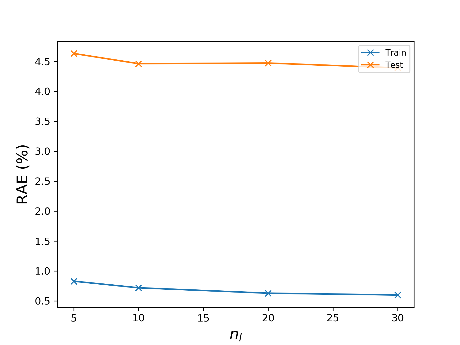
Figure 34: Transient ship airwake: TCAE RAE vs $n_{l}$

Appendix C Training convergence history

Sample convergence histories in the training of different levels of the framework are presented in Fig. 36 to 43. It should be noted that the loss functions are evaluated based on scaled inputs to the networks, thus their values are not to be compared with the MSE given in Sec. 4.

It is observed that the gap between the final training and testing loss increases with the departure of the dynamics between different parameters or time periods. In the discontinuous compressible flow case, the testing loss follows the training loss closely due to the similarity in local dynamics. In contrast, the testing loss saturates noticeably earlier in the other two cases. This is especially clear in the ship airwake TCAE (Fig. 42) due to the significant differences in the patterns of dynamics.

Despite the slower decay in testing error, all errors are below $110-2$ in our tests. In most cases, more than 4 orders of convergence in the training loss is achieved.

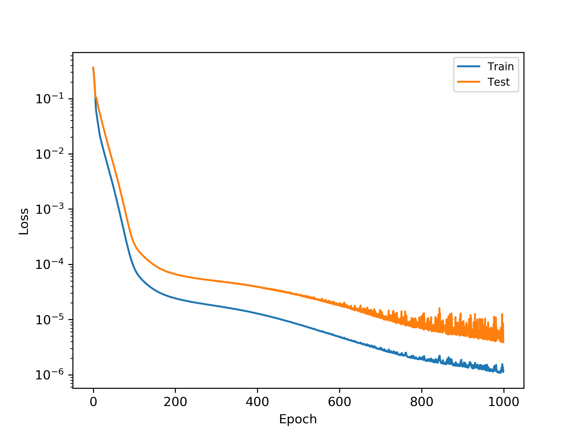
Figure 35: Discontinuous compressible flow: convergence history of CAE

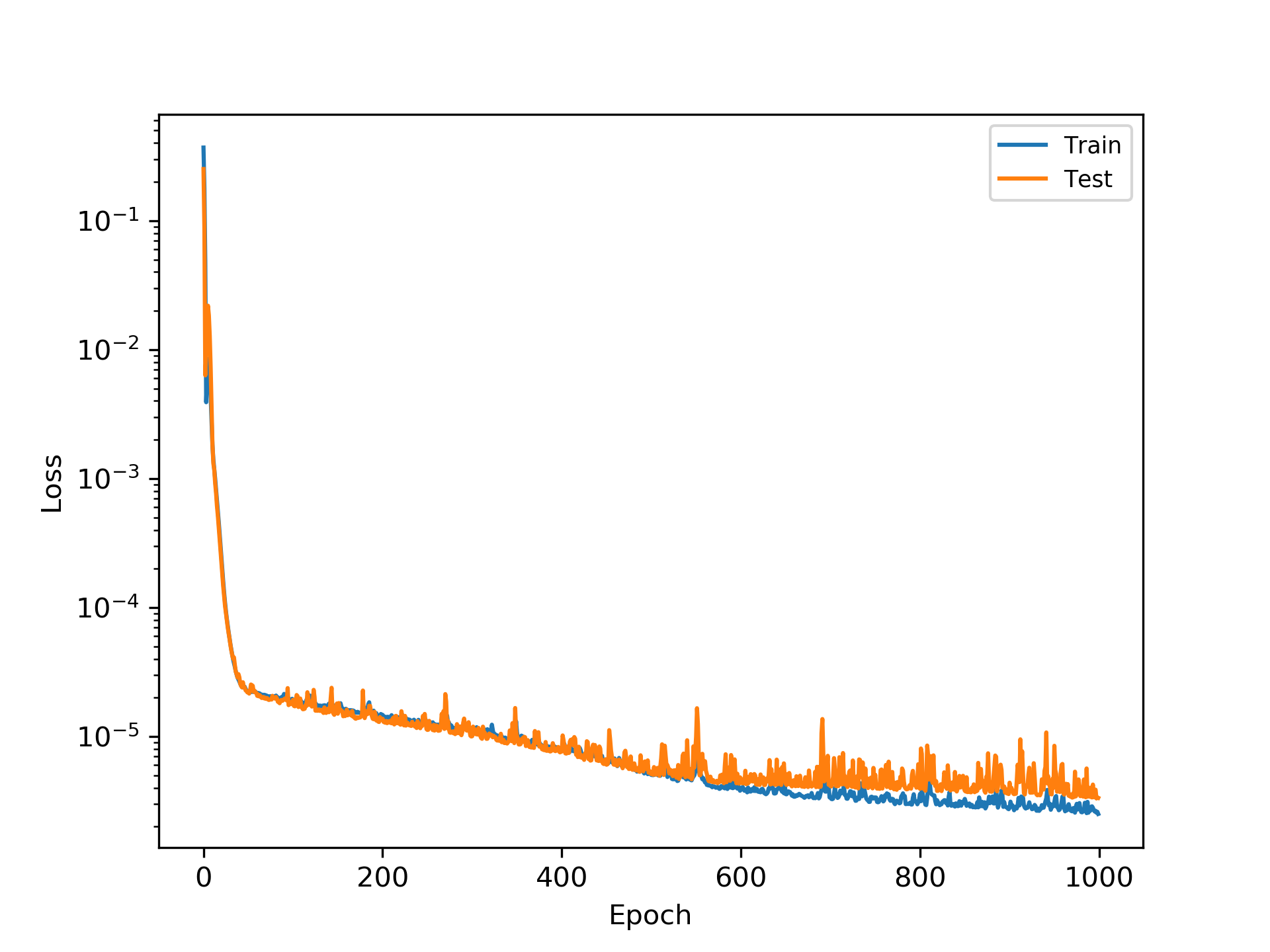
Figure 36: Discontinuous compressible flow: convergence history of TCN

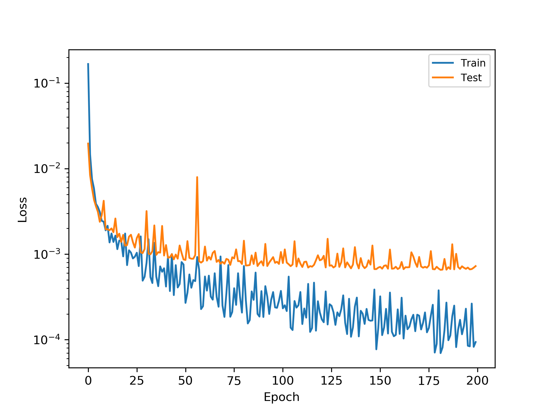
Figure 37: Transient flow over a cylinder: convergence history of CAE

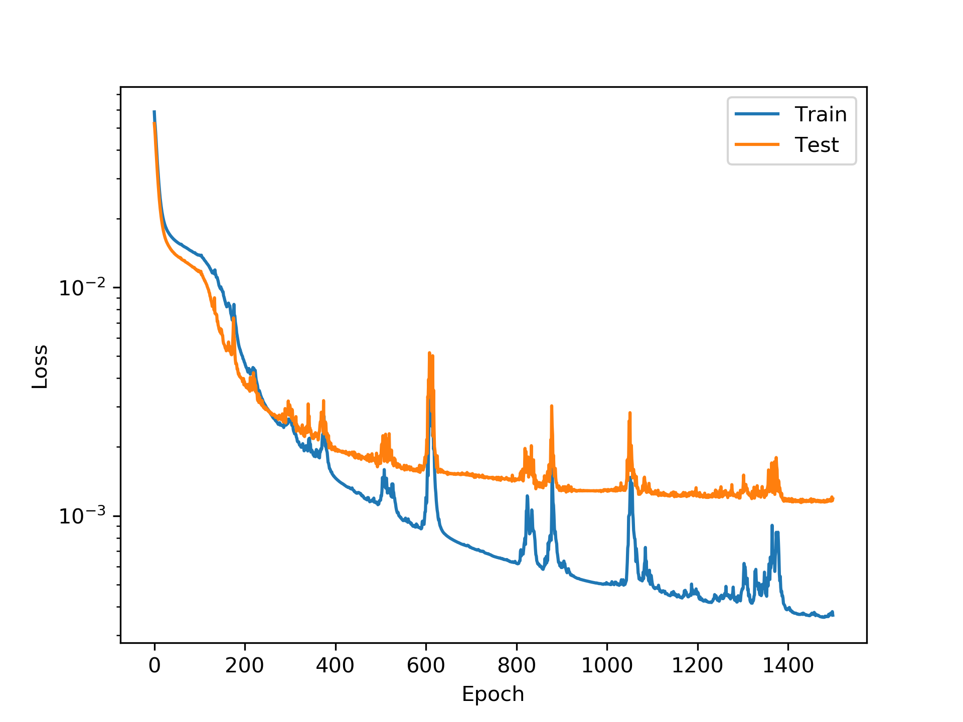
Figure 38: Transient flow over a cylinder: convergence history of TCAE

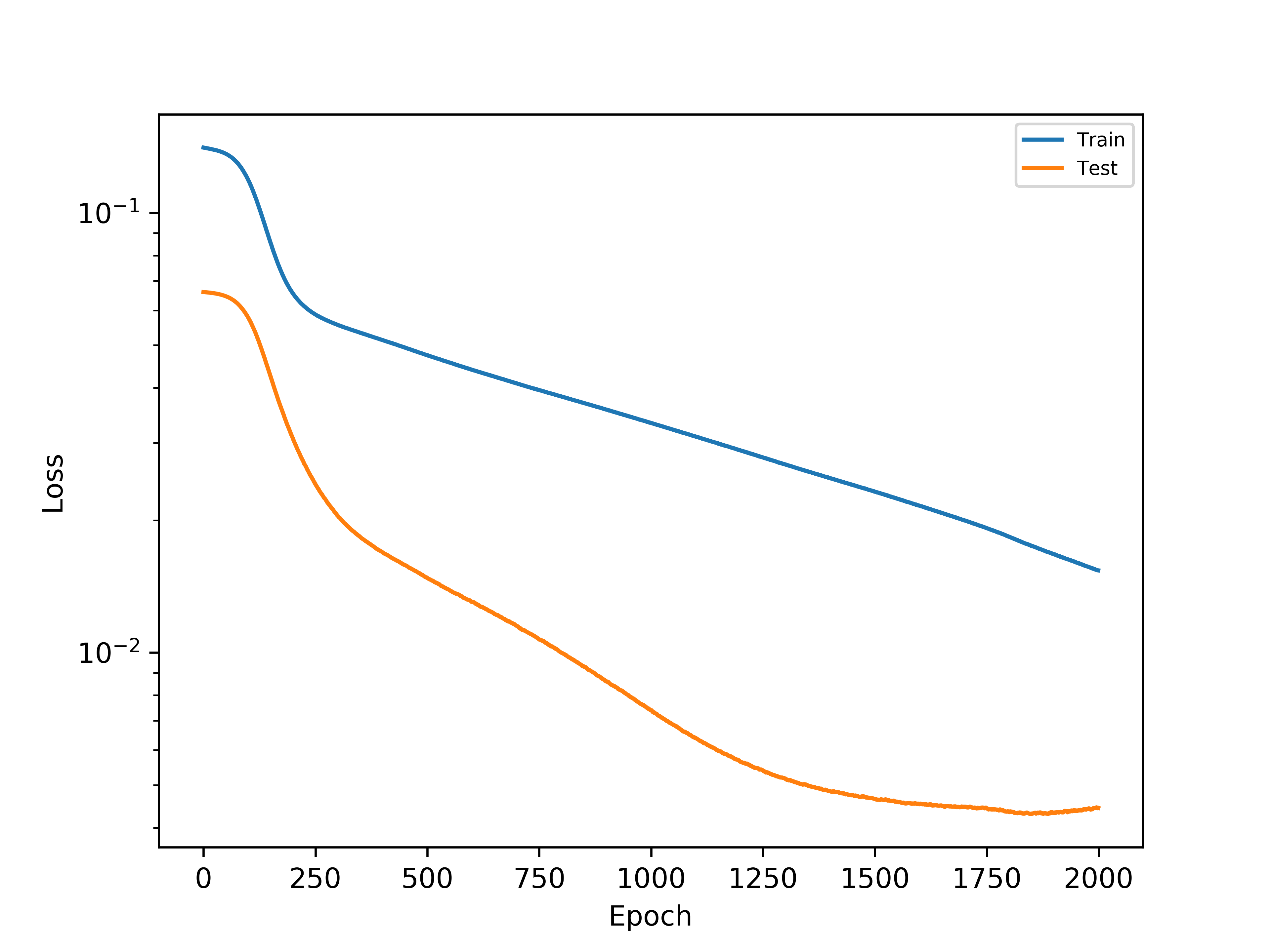
Figure 39: Transient flow over a cylinder: convergence history of MLP

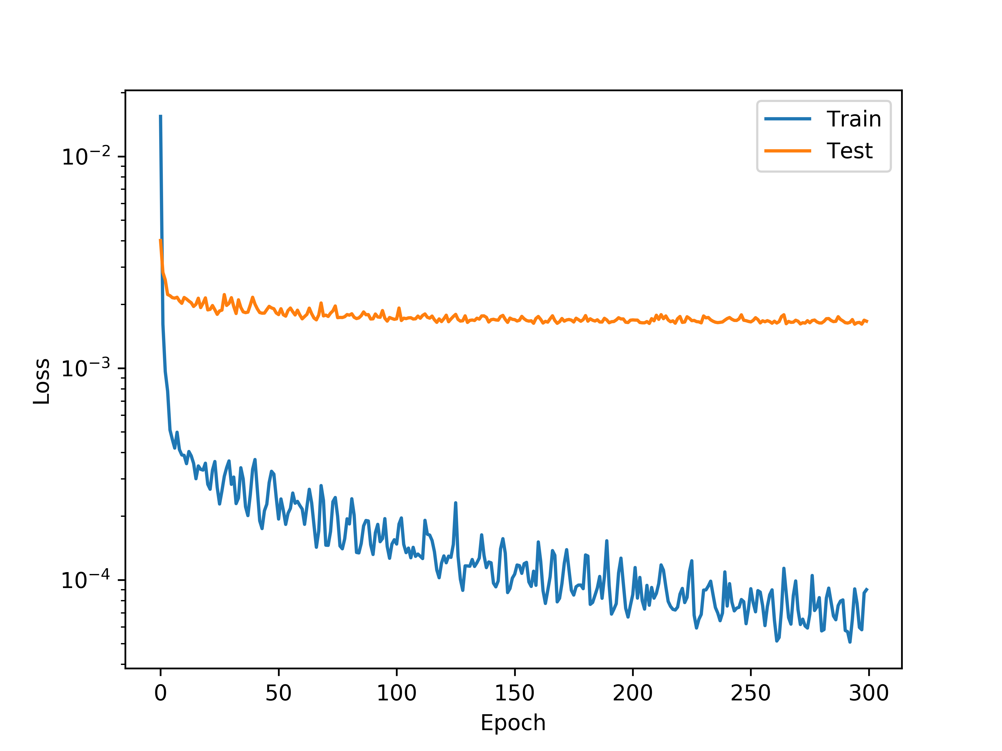
Figure 40: Transient flow over a cylinder: convergence history of TCN

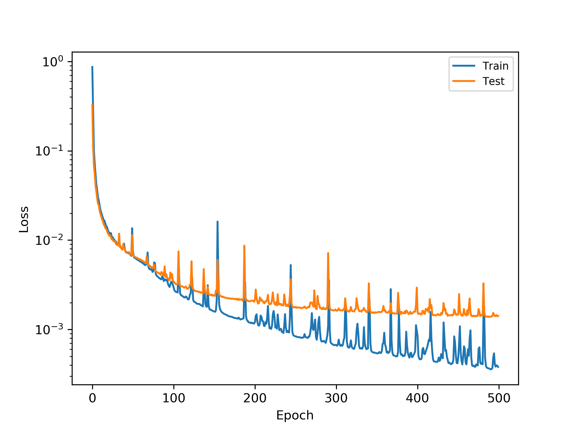
Figure 41: Transient ship airwake: convergence history of CAE

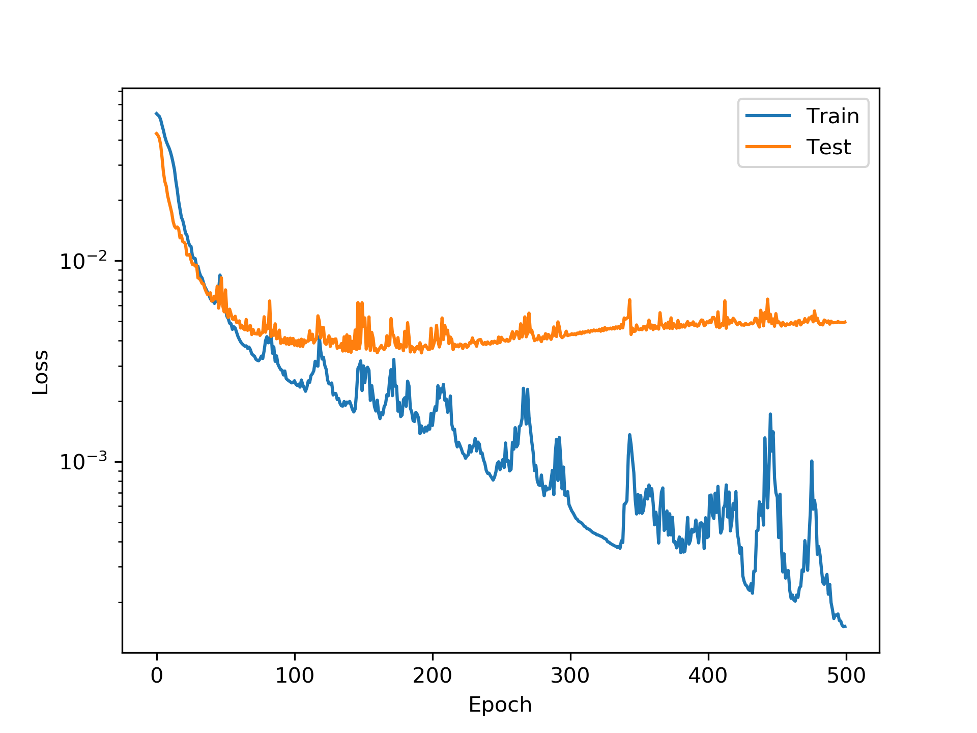
Figure 42: Transient ship airwake: convergence history of TCAE

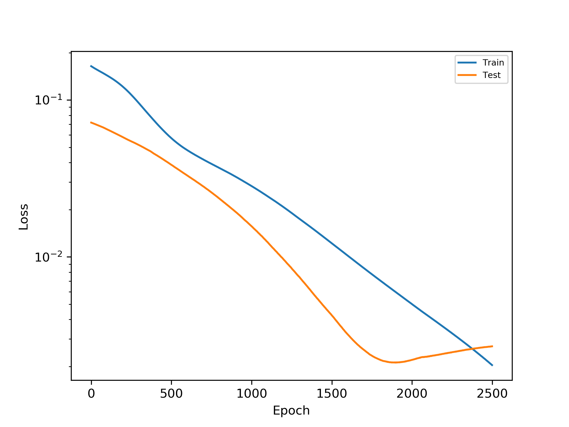
(a)

Figure 43: Transient ship airwake: convergence history of MLP

References

- Benner et al. [2015] P. Benner, S. Gugercin, K. Willcox, A survey of projection-based model reduction methods for parametric dynamical systems, SIAM review 57 (4) (2015) 483–531.
- Berkooz et al. [1993] G. Berkooz, P. Holmes, J. L. Lumley, The proper orthogonal decomposition in the analysis of turbulent flows, Annual review of fluid mechanics 25 (1) (1993) 539–575.
- Rowley et al. [2004] C. W. Rowley, T. Colonius, R. M. Murray, Model reduction for compressible flows using POD and Galerkin projection, Physica D: Nonlinear Phenomena 189 (1-2) (2004) 115–129.
- Moore [1981] B. Moore, Principal component analysis in linear systems: Controllability, observability, and model reduction, IEEE transactions on automatic control 26 (1) (1981) 17–32.
- Safonov and Chiang [1989] M. G. Safonov, R. Chiang, A Schur method for balanced-truncation model reduction, IEEE Transactions on Automatic Control 34 (7) (1989) 729–733.
- Peterson [1989] J. S. Peterson, The reduced basis method for incompressible viscous flow calculations, SIAM Journal on Scientific and Statistical Computing 10 (4) (1989) 777–786.
- Prud’Homme et al. [2001] C. Prud’Homme, D. V. Rovas, K. Veroy, L. Machiels, Y. Maday, A. T. Patera, G. Turinici, Reliable real-time solution of parametrized partial differential equations: Reduced-basis output bound methods, J. Fluids Eng. 124 (1) (2001) 70–80.
- Rozza et al. [2007] G. Rozza, D. B. P. Huynh, A. T. Patera, Reduced basis approximation and a posteriori error estimation for affinely parametrized elliptic coercive partial differential equations, Archives of Computational Methods in Engineering 15 (3) (2007) 1.
- Baur et al. [2011] U. Baur, C. Beattie, P. Benner, S. Gugercin, Interpolatory projection methods for parameterized model reduction, SIAM Journal on Scientific Computing 33 (5) (2011) 2489–2518.
- de Almeida [2013] J. M. de Almeida, A basis for bounding the errors of proper generalised decomposition solutions in solid mechanics, International Journal for Numerical Methods in Engineering 94 (10) (2013) 961–984.
- Berger et al. [2016] J. Berger, S. Gasparin, M. Chhay, N. Mendes, Estimation of temperature-dependent thermal conductivity using proper generalised decomposition for building energy management, Journal of Building Physics 40 (3) (2016) 235–262.
- Rowley [2005] C. W. Rowley, Model reduction for fluids, using balanced proper orthogonal decomposition, International Journal of Bifurcation and Chaos 15 (03) (2005) 997–1013.
- Carlberg et al. [2011] K. Carlberg, C. Bou-Mosleh, C. Farhat, Efficient non-linear model reduction via a least-squares Petrov–Galerkin projection and compressive tensor approximations, International Journal for Numerical Methods in Engineering 86 (2) (2011) 155–181.
- Hijazi et al. [2019] S. Hijazi, G. Stabile, A. Mola, G. Rozza, Data-driven POD-Galerkin reduced order model for turbulent flows, arXiv preprint arXiv:1907.09909 .
- Xu et al. [2019] J. Xu, C. Huang, K. Duraisamy, Reduced-Order Modeling Framework for Combustor Instabilities Using Truncated Domain Training, AIAA Journal (2019) 1–15.
- Huang et al. [2018] C. Huang, J. Xu, K. Duraisamy, C. Merkle, Exploration of reduced-order models for rocket combustion applications, in: 2018 AIAA Aerospace Sciences Meeting, 1183, 2018.
- Carlberg et al. [2017] K. Carlberg, M. Barone, H. Antil, Galerkin v. least-squares Petrov–Galerkin projection in nonlinear model reduction, Journal of Computational Physics 330 (2017) 693–734.
- Wang et al. [2011] Z. Wang, I. Akhtar, J. Borggaard, T. Iliescu, Two-level discretizations of nonlinear closure models for proper orthogonal decomposition, Journal of Computational Physics 230 (1) (2011) 126–146.
- Wang et al. [2012] Z. Wang, I. Akhtar, J. Borggaard, T. Iliescu, Proper orthogonal decomposition closure models for turbulent flows: a numerical comparison, Computer Methods in Applied Mechanics and Engineering 237 (2012) 10–26.
- Parish et al. [2018] E. J. Parish, C. Wentland, K. Duraisamy, The Adjoint Petrov-Galerkin Method for Non-Linear Model Reduction, arXiv preprint arXiv:1810.03455 .
- Gouasmi et al. [2017] A. Gouasmi, E. J. Parish, K. Duraisamy, A priori estimation of memory effects in reduced-order models of nonlinear systems using the Mori–Zwanzig formalism, Proceedings of the Royal Society A: Mathematical, Physical and Engineering Sciences 473 (2205) (2017) 20170385.
- Peherstorfer and Willcox [2015] B. Peherstorfer, K. Willcox, Online adaptive model reduction for nonlinear systems via low-rank updates, SIAM Journal on Scientific Computing 37 (4) (2015) A2123–A2150.
- Peherstorfer [2018] B. Peherstorfer, Model reduction for transport-dominated problems via online adaptive bases and adaptive sampling, arXiv preprint arXiv:1812.02094 .
- Amsallem and Farhat [2011] D. Amsallem, C. Farhat, An online method for interpolating linear parametric reduced-order models, SIAM Journal on Scientific Computing 33 (5) (2011) 2169–2198.
- Hartman and Mestha [2017] D. Hartman, L. K. Mestha, A deep learning framework for model reduction of dynamical systems, in: 2017 IEEE Conference on Control Technology and Applications (CCTA), IEEE, 1917–1922, 2017.
- DeMers and Cottrell [1993] D. DeMers, G. W. Cottrell, Non-linear dimensionality reduction, in: Advances in neural information processing systems, 580–587, 1993.
- Omata and Shirayama [2019] N. Omata, S. Shirayama, A novel method of low-dimensional representation for temporal behavior of flow fields using deep autoencoder, AIP Advances 9 (1) (2019) 015006.
- Lee and Carlberg [2018] K. Lee, K. Carlberg, Model reduction of dynamical systems on nonlinear manifolds using deep convolutional autoencoders, arXiv preprint arXiv:1812.08373 .
- Guo et al. [2016] X. Guo, W. Li, F. Iorio, Convolutional neural networks for steady flow approximation, in: Proceedings of the 22nd ACM SIGKDD International Conference on Knowledge Discovery and Data Mining, ACM, 481–490, 2016.
- Puligilla and Jayaraman [2018] S. C. Puligilla, B. Jayaraman, Deep multilayer convolution frameworks for data-driven learning of fluid flow dynamics, in: 2018 Fluid Dynamics Conference, 3091, 2018.
- Carlberg et al. [2019] K. T. Carlberg, A. Jameson, M. J. Kochenderfer, J. Morton, L. Peng, F. D. Witherden, Recovering missing CFD data for high-order discretizations using deep neural networks and dynamics learning, Journal of Computational Physics .
- Couplet et al. [2005] M. Couplet, C. Basdevant, P. Sagaut, Calibrated reduced-order POD-Galerkin system for fluid flow modelling, Journal of Computational Physics 207 (1) (2005) 192–220.
- Astrid [2004] P. Astrid, Reduction of process simulation models: a proper orthogonal decomposition approach, Technische Universiteit Eindhoven Eindhoven, Netherlands, 2004.
- Astrid et al. [2008] P. Astrid, S. Weiland, K. Willcox, T. Backx, Missing point estimation in models described by proper orthogonal decomposition, IEEE Transactions on Automatic Control 53 (10) (2008) 2237–2251.
- Barrault et al. [2004] M. Barrault, Y. Maday, N. C. Nguyen, A. T. Patera, An ‘empirical interpolation’method: application to efficient reduced-basis discretization of partial differential equations, Comptes Rendus Mathematique 339 (9) (2004) 667–672.
- Chaturantabut and Sorensen [2009] S. Chaturantabut, D. C. Sorensen, Discrete empirical interpolation for nonlinear model reduction, in: Decision and Control, 2009 held jointly with the 2009 28th Chinese Control Conference. CDC/CCC 2009. Proceedings of the 48th IEEE Conference on, IEEE, 4316–4321, 2009.
- Drmac and Gugercin [2016] Z. Drmac, S. Gugercin, A new selection operator for the discrete empirical interpolation method—Improved a priori error bound and extensions, SIAM Journal on Scientific Computing 38 (2) (2016) A631–A648.
- Peherstorfer et al. [2018] B. Peherstorfer, Z. Drmač, S. Gugercin, Stabilizing discrete empirical interpolation via randomized and deterministic oversampling, arXiv preprint arXiv:1808.10473 .
- Brunton et al. [2016] S. L. Brunton, J. L. Proctor, J. N. Kutz, Discovering governing equations from data by sparse identification of nonlinear dynamical systems, Proceedings of the National Academy of Sciences 113 (15) (2016) 3932–3937.
- Gu [2011] C. Gu, QLMOR: A projection-based nonlinear model order reduction approach using quadratic-linear representation of nonlinear systems, IEEE Transactions on Computer-Aided Design of Integrated Circuits and Systems 30 (9) (2011) 1307–1320.
- Kramer and Willcox [2019a] B. Kramer, K. E. Willcox, Nonlinear model order reduction via lifting transformations and proper orthogonal decomposition, AIAA Journal 57 (6) (2019a) 2297–2307.
- Kramer and Willcox [2019b] B. Kramer, K. E. Willcox, Balanced Truncation Model Reduction for Lifted Nonlinear Systems, arXiv preprint arXiv:1907.12084 .
- Schmidt et al. [2011] M. D. Schmidt, R. R. Vallabhajosyula, J. W. Jenkins, J. E. Hood, A. S. Soni, J. P. Wikswo, H. Lipson, Automated refinement and inference of analytical models for metabolic networks, Physical biology 8 (5) (2011) 055011.
- Daniels and Nemenman [2015] B. C. Daniels, I. Nemenman, Automated adaptive inference of phenomenological dynamical models, Nature communications 6 (2015) 8133.
- Barthelmann et al. [2000] V. Barthelmann, E. Novak, K. Ritter, High dimensional polynomial interpolation on sparse grids, Advances in Computational Mathematics 12 (4) (2000) 273–288.
- Guo and Hesthaven [2018] M. Guo, J. S. Hesthaven, Reduced order modeling for nonlinear structural analysis using gaussian process regression, Computer Methods in Applied Mechanics and Engineering 341 (2018) 807–826.
- Hesthaven and Ubbiali [2018] J. S. Hesthaven, S. Ubbiali, Non-intrusive reduced order modeling of nonlinear problems using neural networks, Journal of Computational Physics 363 (2018) 55–78.
- Wang et al. [2019] Q. Wang, J. S. Hesthaven, D. Ray, Non-intrusive reduced order modeling of unsteady flows using artificial neural networks with application to a combustion problem, Journal of computational physics 384 (2019) 289–307.
- Mohan et al. [2019] A. Mohan, D. Daniel, M. Chertkov, D. Livescu, Compressed convolutional LSTM: An efficient deep learning framework to model high fidelity 3D turbulence, arXiv preprint arXiv:1903.00033 .
- Lee and You [2018] S. Lee, D. You, Data-driven prediction of unsteady flow fields over a circular cylinder using deep learning, arXiv preprint arXiv:1804.06076 .
- Rumelhart et al. [1988] D. E. Rumelhart, G. E. Hinton, R. J. Williams, et al., Learning representations by back-propagating errors, Cognitive modeling 5 (3) (1988) 1.
- Hochreiter and Schmidhuber [1997a] S. Hochreiter, J. Schmidhuber, LSTM can solve hard long time lag problems, in: Advances in neural information processing systems, 473–479, 1997a.
- Gonzalez and Balajewicz [2018] F. J. Gonzalez, M. Balajewicz, Deep convolutional recurrent autoencoders for learning low-dimensional feature dynamics of fluid systems, arXiv preprint arXiv:1808.01346 .
- Maulik et al. [2020] R. Maulik, A. Mohan, B. Lusch, S. Madireddy, P. Balaprakash, D. Livescu, Time-series learning of latent-space dynamics for reduced-order model closure, Physica D: Nonlinear Phenomena (2020) 132368.
- Xingjian et al. [2015] S. Xingjian, Z. Chen, H. Wang, D.-Y. Yeung, W.-K. Wong, W.-c. Woo, Convolutional LSTM network: A machine learning approach for precipitation nowcasting, in: Advances in neural information processing systems, 802–810, 2015.
- Yu et al. [2017] B. Yu, H. Yin, Z. Zhu, Spatio-temporal graph convolutional networks: A deep learning framework for traffic forecasting, arXiv preprint arXiv:1709.04875 .
- Elman [1990] J. L. Elman, Finding structure in time, Cognitive science 14 (2) (1990) 179–211.
- Hochreiter and Schmidhuber [1997b] S. Hochreiter, J. Schmidhuber, Long short-term memory, Neural computation 9 (8) (1997b) 1735–1780.
- Cho et al. [2014] K. Cho, B. Van Merriënboer, D. Bahdanau, Y. Bengio, On the properties of neural machine translation: Encoder-decoder approaches, arXiv preprint arXiv:1409.1259 .
- Wang et al. [2016] Y. Wang, M. Huang, X. Zhu, L. Zhao, Attention-based LSTM for aspect-level sentiment classification, in: Proceedings of the 2016 conference on empirical methods in natural language processing, 606–615, 2016.
- Wu et al. [2016] Y. Wu, M. Schuster, Z. Chen, Q. V. Le, M. Norouzi, W. Macherey, M. Krikun, Y. Cao, Q. Gao, K. Macherey, et al., Google’s neural machine translation system: Bridging the gap between human and machine translation, arXiv preprint arXiv:1609.08144 .
- Qing and Niu [2018] X. Qing, Y. Niu, Hourly day-ahead solar irradiance prediction using weather forecasts by LSTM, Energy 148 (2018) 461–468.
- Rather et al. [2015] A. M. Rather, A. Agarwal, V. Sastry, Recurrent neural network and a hybrid model for prediction of stock returns, Expert Systems with Applications 42 (6) (2015) 3234–3241.
- Eck and Schmidhuber [2002] D. Eck, J. Schmidhuber, A first look at music composition using lstm recurrent neural networks, Istituto Dalle Molle Di Studi Sull Intelligenza Artificiale 103 (2002) 48.
- Oord et al. [2016] A. v. d. Oord, S. Dieleman, H. Zen, K. Simonyan, O. Vinyals, A. Graves, N. Kalchbrenner, A. Senior, K. Kavukcuoglu, Wavenet: A generative model for raw audio, arXiv preprint arXiv:1609.03499 .
- Bai et al. [2018] S. Bai, J. Z. Kolter, V. Koltun, An empirical evaluation of generic convolutional and recurrent networks for sequence modeling, arXiv preprint arXiv:1803.01271 .
- Gehring et al. [2016] J. Gehring, M. Auli, D. Grangier, Y. N. Dauphin, A convolutional encoder model for neural machine translation, arXiv preprint arXiv:1611.02344 .
- Lea et al. [2017] C. Lea, M. D. Flynn, R. Vidal, A. Reiter, G. D. Hager, Temporal convolutional networks for action segmentation and detection, in: proceedings of the IEEE Conference on Computer Vision and Pattern Recognition, 156–165, 2017.
- Dauphin et al. [2017] Y. N. Dauphin, A. Fan, M. Auli, D. Grangier, Language modeling with gated convolutional networks, in: International conference on machine learning, 933–941, 2017.
- He et al. [2015] K. He, X. Zhang, S. Ren, J. Sun, Delving deep into rectifiers: Surpassing human-level performance on imagenet classification, in: Proceedings of the IEEE international conference on computer vision, 1026–1034, 2015.
- Dumoulin and Visin [2016] V. Dumoulin, F. Visin, A guide to convolution arithmetic for deep learning, arXiv preprint arXiv:1603.07285 .
- Kingma and Ba [2014] D. P. Kingma, J. Ba, Adam: A method for stochastic optimization, arXiv preprint arXiv:1412.6980 .
- Sod [1978] G. A. Sod, A survey of several finite difference methods for systems of nonlinear hyperbolic conservation laws, Journal of computational physics 27 (1) (1978) 1–31.
- Danaila et al. [2007] I. Danaila, P. Joly, S. M. Kaber, M. Postel, Gas Dynamics: The Riemann Problem and Discontinuous Solutions: Application to the Shock Tube Problem, in: Introduction to scientific computing, Springer, New York, NY, 213–233, 2007.
- Parish and Carlberg [2019] E. J. Parish, K. T. Carlberg, Time-series machine-learning error models for approximate solutions to parameterized dynamical systems, arXiv preprint arXiv:1907.11822 .
- Huang et al. [2019] C. Huang, K. Duraisamy, C. L. Merkle, Investigations and improvement of robustness of reduced-order models of reacting flow, AIAA Journal 57 (12) (2019) 5377–5389.
- Lee et al. [2005] D. Lee, N. Sezer-Uzol, J. F. Horn, L. N. Long, Simulation of helicopter shipboard launch and recovery with time-accurate airwakes, Journal of Aircraft 42 (2) (2005) 448–461.
- Wilcox [1988] D. C. Wilcox, Reassessment of the scale-determining equation for advanced turbulence models, AIAA journal 26 (11) (1988) 1299–1310.
- Huang et al. [2020] C. Huang, K. Duraisamy, C. Merkle, Data-Informed Species Limiters for Local Robustness Control of Reduced-Order Models of Reacting Flow, in: AIAA Scitech 2020 Forum, 2141, 2020.
- Raissi et al. [2019] M. Raissi, P. Perdikaris, G. E. Karniadakis, Physics-informed neural networks: A deep learning framework for solving forward and inverse problems involving nonlinear partial differential equations, Journal of Computational Physics 378 (2019) 686–707.
- Pan and Duraisamy [2020] S. Pan, K. Duraisamy, Physics-Informed Probabilistic Learning of Linear Embeddings of Non-linear Dynamics With Guaranteed Stability, SIAM Journal on Applied Dynamical Systems, arXiv preprint arXiv:1906.03663 .
- Swischuk et al. [2019] R. Swischuk, B. Kramer, C. Huang, K. Willcox, Learning physics-based reduced-order models for a single-injector combustion process, arXiv preprint arXiv:1908.03620 .
- Gin et al. [2019] C. Gin, B. Lusch, S. L. Brunton, J. N. Kutz, Deep Learning Models for Global Coordinate Transformations that Linearize PDEs, arXiv preprint arXiv:1911.02710 .
- Kipf and Welling [2016] T. N. Kipf, M. Welling, Semi-supervised classification with graph convolutional networks, arXiv preprint arXiv:1609.02907 .