Probabilistic Simulation of Quantum Circuits with the Transformer
Abstract
The fundamental question of how to best simulate quantum systems using conventional computational resources lies at the forefront of condensed matter and quantum computation. It impacts both our understanding of quantum materials and our ability to emulate quantum circuits. Here we present an exact formulation of quantum dynamics via factorized generalized measurements which maps quantum states to probability distributions with the advantage that local unitary dynamics and quantum channels map to local quasi-stochastic matrices. This representation provides a general framework for using state-of-the-art probabilistic models in machine learning for the simulation of quantum many-body dynamics. Using this framework, we have developed a practical algorithm to simulate quantum circuits with the Transformer, a powerful ansatz responsible for the most recent breakthroughs in natural language processing. We demonstrate our approach by simulating circuits which build GHZ and linear graph states of up to 60 qubits, as well as a variational quantum eigensolver circuit for preparing the ground state of the transverse field Ising model on six qubits. Our methodology constitutes a modern machine learning approach to the simulation of quantum physics with applicability both to quantum circuits as well as other quantum many-body systems.
In his celebrated keynote address at the California Institute of Technology in May 1981, Feynman introduced the idea of a computer that could act as a quantum mechanical simulator,Feynman (1982) which has inspired the field of quantum computing since its inception. In his keynote, Feynman also intriguingly asked “can quantum systems be probabilistically simulated by classical computer?”, which he answered negatively observing that a probabilistic simulation is unfeasible since the description of both the quantum state and its evolution necessarily involves non-positive quasi-probabilities.
These simple but powerful observations provide a glimpse into the boundary of what behaviour can be considered classical or quantum, since classical systems are fully characterized by traditional probability distributions evolving according to non-negative stochastic matrices.Domb (2000) From a computational viewpoint, these observations are also fundamentally linked to the notion of quantum speed-up in quantum computing, where it is anticipated that quantum computers will display potential speed-ups over their classical counterparts at the onset of negative values in the quasi-probabilities associated with the description and evolution of their quantum states.Ferrie (2011); Veitch et al. (2012); Raussendorf et al. (2019) This is in part due to the negative values in the quasi-probability distributions precluding an efficient simulation of quantum dynamics through Monte Carlo techniques due to the debilitating sign problem induced by the negative values.
Although the presence of negative quasi-probabilities is often linked to intrinsically quantum phenomena with no classical counterpart like entanglement and quantum interference, a purely probabilistic representation of the quantum state is possible.Fuchs and Schack (2011); Chruściński et al. (2015); van de Wetering (2018); Carrasquilla et al. (2019); Kiktenko et al. (2019) While in the standard formulation of quantum mechanics a quantum state is represented by a density operator, a quantum state can also be completely specified by the outcome probability of a physical measurement, provided that the measurement probes enough information about the quantum state. This notion is made precise through two fundamental concepts in quantum theory: the so-called Born rule, which is the theoretical principle of quantum physics linking quantum theory and experiment, and the concept of informationally complete (IC) measurements, which are described by positive-operator valued measures (POVMs). Whereas POVMs describe the most general type of measurements allowed by quantum theory going beyond the notion of projective measurements, Nielsen and Chuang (2011) informational completeness means that the outcome statistics of such a measurement specifies the quantum state unambiguously.
Recently, neural probabilistic models (NPM) that are commonly used in language modelling and translation have been used in the context of quantum state reconstruction.Carrasquilla et al. (2019) Such a strategy resulted in an accurate probabilistic representation of families of prototypical states in quantum information as well as complex ground states of one- and two-dimensional local Hamiltonians describing large many-body systems relevant to condensed matter, cold atomic systems, and quantum simulators.Carrasquilla et al. (2019) Although an exact simulation of quantum dynamics using probability remains, in general, unfeasible, it is natural to ask whether the power and scalability of the neural probabilistic representation of the quantum state in Ref. Carrasquilla et al., 2019, can be harnessed in the classical simulation of quantum systems, e.g. in challenging scenarios like the study of real- and imaginary-time dynamics of many-body systems, or in the classical simulation of quantum circuits and quantum channels.
Inspired by Feynman’s notion of a probabilistic simulation of quantum systems, we employ a probabilistic representation of the quantum state and combine it with state-of-the-art neural language modelling architectures to approximate the statistics of the measurement outcome of states produced by quantum circuits. The near-term availability of quantum computers with the potential to perform computational tasks beyond the capabilities of the most powerful classical computersBouland et al. (2018) has given rise to a new generation of exact and approximate classical simulation techniquesDe Raedt et al. (2007); Markov and Shi (2008); Smelyanskiy et al. (2016); Pednault et al. (2017); Chen et al. (2018); Markov et al. (2018); Li et al. (2018) for quantum circuits, including a neural network approach.Jónsson et al. (2018) We test our ideas by considering quantum circuits which prepare prototypical states in quantum information. In particular we consider the GHZ state, linear graph state, and the variational ground state of the transverse field Ising model (TFIM). Through numerical experiments, we show that our strategy produces accurate results for the target states of up to 60 qubits, which opens up a new probabilistic avenue for simulation of quantum circuits, as well as quantum channels and quantum dynamics more broadly.
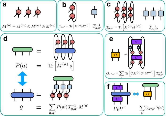
Formalism: We focus on physical systems composed of qubits whose quantum state, traditionally represented by a density matrix , will be uniquely specified by the measurement statistics of an informationally complete POVM (IC-POVM). To build an IC-POVM for qubits, we first consider an -outcome single-qubit IC-POVM defined by a collection , of positive semi-definite operators , each one labeled by a measurement outcome [see Fig.1(a) where we describe our representation through the lens of tensor networks and its graphical notation.Penrose (1971)] Following Ref. Carrasquilla et al., 2019, we construct -qubit measurements as tensor products of the single-qubit IC-POVM elements , as graphically depicted in Fig.1(a). Due to the simplicity of its implementation with currently available gate-based quantum computers, in our numerical simulations we consider the 4-Pauli IC-POVM measurement described in Ref.Carrasquilla et al., 2019. Born’s rule predicts that the probability distribution over measurement outcomes on a quantum state is given by , as graphically explained in Fig.1(d). Note that a quantum state is specified by probabilities. Due to the factorized nature of the IC-POVM, a product state takes the form of a product distribution over statistically independent sets of variables where . Provided that the measurement is informationally complete, the density matrix can be inferred from the statistics of the measurement outcome as
| (1) |
where represents the overlap matrix given by . See Fig.1(d) for a graphical representation of elements in Eq.1.
To study quantum circuits, we first have to translate the action of a quantum gate on the density matrix to the IC-POVM representation. The former corresponds to a unitary transformation, i.e. . If the initial quantum state is prescribed in terms of the outcome statistics of an IC-POVM , we can track its evolution directly in the probabilistic representation:
| (2) |
where
| (3) |
is a somewhat stochastic matrix since the values in each column add up to 1 but its entries can be positive or negative.Ćurgus and Jewett (2007, 2015); Chruściński et al. (2015); van de Wetering (2018) Somewhat stochastic matrices are also known as pseudo-stochastic or quasi-stochastic matrices.Chruściński et al. (2015); van de Wetering (2018) We note that the evolution described in Eq. 2 leads to a formulation of quantum mechanics equivalent to, e.g. Heisenberg’s matrix mechanics, including the description of open quantum systems, quantum channels, and measurements of other POVMs (See Appendix).
Here we emphasize that Eq. 2 resembles the standard rule for stochastic evolution commonly used to describe the transitions in a Markov chain, where the traditional stochastic (or Markov) matrix has been replaced with a quasi-stochastic matrix. Despite the resemblance, a generic classical Markov Chain Monte Carlo simulation of quantum evolution in the probabilistic factorized POVM language remains unfeasible due to the numerical sign problem arising from the negative entries of the quasi-stochastic matrix describing the process.
Due to the factorized nature of the IC-POVM, if a unitary matrix or a quantum channel acts nontrivially on only qubits of the quantum system, the quasi-stochastic matrix acts only on the measurement outcomes of those qubits too. For example, a two-qubit unitary gate acting on qubits and is represented by a quasi-stochastic matrix acting on outcomes and . The relation between the local quasi-stochastic matrices and the local unitary gates, as well as their action on a quantum state are graphically depicted in Fig.1(e-f) using tensor diagrams. Furthermore, the locality of implies that traditional quantum circuit diagramsNielsen and Chuang (2011) translate into probabilistic circuits that look exactly the same as their traditional counterparts.
A quantum circuit is a generalization of the circuit model of classical computation where a product state is evolved through a series of unitary gates, , each of which acts nontrivially on a constant number qubits. Thus, the quantum circuit in the IC-POVM representation becomes a computation where an initial probability distribution of statistically independent sets of variables which is evolved through a series of local quasi-stochastic matrices of the form depicted in Fig.1(e). The measurement statistics after unitary evolution through the first gate is given by , and the application of each subsequent gate defines a series of intermediate probability distributions with .
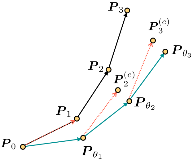
Algorithm: The strategy to learn the output distribution consists in constructing models based on a rich family of probability distributions . These are expressed in terms of a highly expressive neural network with parameters so that . At each time step , we assume that an accurate neural approximation has been reached , and consider the exactly evolved distribution . While the representation of the quantum state at step isn’t exact, if is sufficiently accurate the expectation is that the distribution . See Fig. 2 for a depiction of the distributions involved during the simulation.
To train the model given a gate , we adopt a variational approach and select the parameters such that the Kullback-Liebler (KL) divergence between and ,
| (4) |
is minimized. This objective function is reasonable as , with the equality being satisfied when . To minimize the KL divergence, we will apply a variant of gradient descent (i.e. ADAMKingma and Ba (2015)) where we repeatedly update the parameters of by taking steps in the direction of the gradient of Eq. 4. This gradient, assuming that the model is normalized, can be written as
| (5a) | ||||
| (5b) | ||||
| (5c) | ||||
| (5d) | ||||
Here, . Note that , which justifies the equality in Eq. 5d. To estimate the gradient in Eq. 5a, we generate a mini-batch of samples of sampled from and average over these samples both to compute the value of as well as Eq. 5d. While computing Eq. 5d or Eq. 5c both evaluate the gradient, Eq. 5d has significantly better variance. In the limit where approaches (i.e. ideally towards the end of the optimization of gate ), the variance of this gradient goes to zero. This is known as the zero variance principle. Assaraf and Caffarel (1999) is evaluated by explicitly summing over the sub-string of outcomes in on which acts (with the other outcomes in the string fixed).
By construction, the unitary matrices and their corresponding quasi-stochastic matrices considered here are -local, which means that the calculation of the gradient estimator in Eq. 5a is efficient.
Transformer: For simplicity, in order to model , we restrict to models with a tractable density and that allow for exact sampling. While other models such as the variational autoencoderLuchnikov et al. (2019) can represent the quantum state probabilistically, having both a tractable density and exact sampling significantly simplifies the calculation of the quantities involved in the gradient estimation. The exact sampling avoids expensive Markov Chain Monte Carlo which would otherwise be required to obtain the samples for the gradient estimator. Specifically, we consider prototypical autoregressive models commonly used in neural machine translation and language modelling based on Transformer encoder blocks.Vaswani et al. (2017) This neural architecture models a probability distribution through the conditional . Note that we can recover via the chain rule
which we heavily use in our simulations.
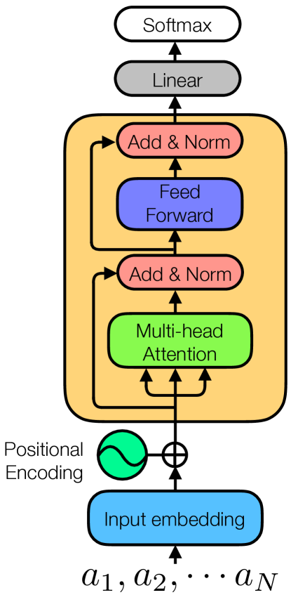
The Transformer architecture is constructed using the elements depicted in Fig. 3. The first and most important element is the self-attention mechanism. Self-attention takes an embedding of the measurement outcome , and computes an auto-correlation matrix where the different measurement outcomes across the different qubits form the columns and rows. The embedding is simply a linear transformation on the original input . The self-attention and its correlation matrix are useful to introduce correlations between qubits separated at any distance in the quantum system. This is analogous to a two-body Jastrow factorBecca and Sorella (2017) which induces pairwise long-distance correlations between the bare degrees of freedom (i.e. spins, qubits, electrons) in a wavefunction. In contrast to traditional sequence models based on recurrent neural networks, which tend to suppress correlations beyond a certain length , the self-attention networks are suitable to model systems exhibiting power-law correlations present in natural sequences as well as physical systems exhibiting (classical or quantum) critical behaviour.Shen (2019)
More precisely, the attention mechanism can be described as a map between a “query” array , a “key” array and “value” , to an output vector. The the query, keys, values, are linear transformations of the input vectors, e.g. , where is a -dimensional embedding of the measurements outcome at the different qubits , and is a parameter of the model. Analogously, the values and queries are calculated as a parametrized linear transformation on the embedding .
The specific type of attention mechanism the Transformer uses is the so-called scaled dot-product attention. The input consists of queries and keys of dimension , and values of dimension , and the output is computed as
| (6) |
where the softmax function acting on a vector results in . The argument of the softmax is , which induces pairwise, all-to-all correlations between the qubits in the system, thus resembling a Jastrow factor with parameters .
As in Ref. Vaswani et al., 2017, we use a multi-head attention mechanism where instead of computing a single attention function, we linearly project the queries, keys and values times with different, learned linear projections to , and dimensions. Each of these projections are then followed by the attention function in parallel, producing -dimensional output values. These are concatenated and projected. The output of the multi-head attention is
| (7) |
where , , , and . Here, , , and . In our work we use attention heads, and with or 32.
Additionally, the Transformer features a position-wise feed-forward network, which is a fully connected feed-forward network applied to each position separately and identically. This layer consists of two linear transformations with a ReLUGoodfellow et al. (2016) activation in between.
Each sub-layer (i.e. the self-attention and the position-wise feed-forward network) has a residual connection around it, and is followed by a layer-normalization step. That is, the output of each sub-layer is , where is the function implemented by either the self-attention or the position-wise feed-forward network. The residual connectionHe et al. (2015) makes it simple for the architecture to perform the identity operation on the input since can easily be trained to output zeros. The layer normalizationBa et al. (2016) is a technique to normalize the of intermediate outcome of the sub-layers to have zero mean and unit variance, which enables a more stable calculation of the gradients in Eq.5a and faster training.
The embedding mentioned above convert the values of measurements to vectors of dimension through a parametrized linear transformation. Since the Transformer model contains no recurrence or convolutions, the model can’t naturally use the information of the the spatial ordering of the qubits. To fix this, we include information about the relative or absolute position of the measurements in the system by adding positional encodings to the input embeddings. The positional encodings have the same dimension as the embeddings and are added to the original embedding.Vaswani et al. (2017) The last element of the Transformer is a linear layer followed by a softmax activation that outputs the conditional distribution.
While several Transformer layers of the type encircled in the orange block in Fig. 3 can be composed to enhanced the expressiveness of our models, we found that the one-layer Transformer-encoder architecture described above suffices for modeling distributions we are interested in. We train the models using Adam OptimizerKingma and Ba (2015) in Pytorch Paszke et al. (2017) with an initial learning rate of 0.01. Our implementation uses single-precision (32-bit) floating-point representation for real numbers and a 64-bit representation for integers.
Experiments and results: We demonstrate our approach on three types of quantum circuits: circuits producing GHZ states, circuits producing one-dimensional graph states, and a variational circuit for the ground state of the Transverse Ising Field Model at the critical point Ho and Hsieh (2019) (see Appendix). We use a variety of quality metrics to quantify the efficacy of our method: The KL divergence of Eq. 4, the classical fidelity , and the norm of the probability distributions are all designed to measure the difference between the probability distribution of the neural probabilistic model and the exact probability distribution (either or ) of the POVM. Note that these measures directly bound how far off the POVM measurement statistics of the actual quantum state differ from our simulation. These measures depend on the POVM basis; we can also directly compare basis-independent quantities such as the ‘quantum fidelity’ of the state,
| (8) |
and
| (9) |
Both and are equal to the overlap when and represent pure states. Notice that is well defined even if the ‘density matrices’ generated from the POVM probability don’t correspond to physical density matrices.
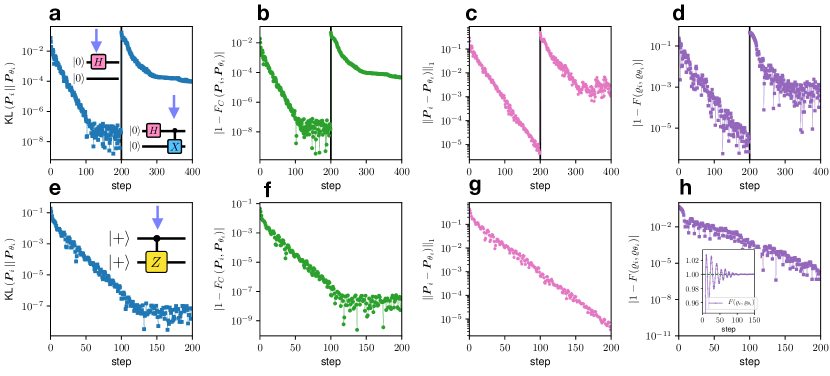
Fig.4(a-d) shows these measures for two quantum gates (see Fig.4(a)[inset]) which generate the GHZ state with qubits, namely the Bell state . For the application of each of the two gates, the KL divergence, the L1 classical error, the classical fidelity error, and the quantum fidelity error all initially approach zero exponentially in the number of steps. The quantum fidelity oscillates around one until finally settling at 1 by the end of the optimization. The KL divergence and the classical fidelity error both eventually saturate, but, interestingly, the L1 classical error and the quantum fidelity error both continue to improve for the application of the first gate in the circuit. This suggests that further improvements due to better training of the ansatz and a better choice of objective function are possible. The observed saturation at also suggests some quantities are limited by the 32-bit floating-point precision used in computations. Increasing the precision could also lead to improved convergence. In Fig. 4(e-h), we present analogous results for a circuit generating a -qubit graph state, i.e. , where we observe similar behaviour. Note that for these examples, we are primarily probing the quality of our optimization given that the Transformer with hidden dimension 16 should be powerful enough to exactly represent the exact probability distribution.
The small oscillations of the fidelity above 1.0 evident in the inset of Fig. 4(h) exists because the Transformer can represent probability distributions without a corresponding physical density matrix. This is because only a subset of the probability simplex, which is the space where the distributions we are interested in live, corresponds to physical density matrices upon inversion in Eq.1. The subset of probability distributions with a valid quantum states in our setting forms a convex set similar to the so-called Qplex in quantum Bayesian theory.Appleby et al. (2017) Here we emphasize that the fidelity values in Fig.4(d) and (h) eventually converge to one and the oscillations above and below 1 are suppressed exponentially with the training steps, suggesting that the model converges to the target quantum state. We provide more details about the Qplex and the presence of unphysical states in our representation in the Appendix.
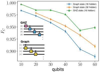
We now turn our attention to the quality of the circuit simulation as a function of the number of qubits in the circuit, letting both the depth and gate number grow linearly with the number of qubits. We find in constructing GHZ and linear graph states (see Fig. 5(inset)) in the range from 10-60 qubits that the classical fidelity falls approximately linearly with number of qubits (see Fig. 5) reaching a classical fidelity of approximately 0.9 at 60 qubits. In addition, we have considered two different hidden dimensions, 16 and 32, and find that there is an improvement of the classical fidelity over all qubit sizes as we increase the hidden dimension. We attribute this to an improved representability power of the larger Transformers suggesting that one of the bottlenecks of our simulation is the ability of our neural probabilistic model to represent the probability distribution that corresponds to the output of the quantum circuit.
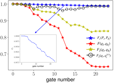
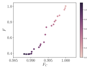
We further apply our method for state preparation of a 6-qubit TFIM ground state using a variational quantum eigensolver circuit Ho and Hsieh (2019) (see Appendix). The variational quantum eigensolver Peruzzo et al. (2014) (VQE) is a quantum/classical hybrid algorithm that can be used to approximate the lowest energy eigenvalues and eigenvectors of a qubit Hamiltonian on a quantum processor. Rather than performing an optimization of the VQE ansatz, we focus on the probabilistic preparation of an already optimized VQE circuit for the ground state of the TFIM, as demonstrated below. We note that the particular circuit we consider has more gates per qubit than our previous examples. However, we limit our simulation to a small number of qubits so that the estimation of quantum fidelity, whose computational cost is exponential in the number of qubits in our approach,Carrasquilla et al. (2019) remains possible. Thus we evaluate both classical and quantum fidelity after the application of each quasi-stochastic gate in the circuit (see Appendix F for a precise specification of the quantum circuit and details of its probabilistic preparation). Both the classical and quantum fidelities shown in Fig. 6 drop roughly linearly with the number of gates in the circuit; in fact, as demonstrated in the Appendix in Fig. A5, there is a clear correlation between the classical and quantum fidelity. It is natural to expect that this linear drop observed in our simulation is brought on by an accumulation of errors building up after successive gates in the circuit. We can give further evidence of this by looking at the error made after a single step, , which directly compares and (see Fig. 6). We find that the single-step error is roughly constant and small throughout the circuit suggesting each step of the simulation is fairly accurate. This is consistent with the observations in Fig. 4.
Conclusions: We have introduced an approach for the classical simulation of quantum circuits using probabilistic models and validate it on a number of different circuits. This is done by using a POVM formalism which maps states to probability distributions and gates to quasi-stochastic matrices. To represent the probability distribution over this POVM basis, we use a Transformer, a powerful machine learning architecture heavily used in natural language processing. We develop an efficient sampling scheme which updates the Transformer after each gate application within the quantum circuit. This sampling scheme works well out to a large number of qubits; in this work we demonstrate simulations up to 60 qubits and empirically see that the accuracy of the simulation drops roughly linearly with the number of qubits at a fixed hidden dimension of the Transformer architecture. We observe that increasing the hidden dimension of the model improves our results for the circuits we considered. Although this observation suggests that our approach is scalable, a detailed study of the representational power of the Transformer and its relation to optimization over a wider class of circuits and Transformer hyperparameters is required to properly establish the scalability and applicability of our approach.
Optimizing the Transformer after each gate is a critical step in our algorithm. While already reasonably efficient, there are various ways this optimization might be further improved. For example, our current simulations allow probabilistic representations which don’t map to physical quantum states (i.e. outside of the Qplex). We anticipate that constraining the optimization to the physically relevant subspace would improve the quality of the simulations and their broad applicability. Additionally, further strategies from machine learning may be applicable; a common training strategy in natural language processing has been to simultaneously train multiple models selecting the best one at each step and this technique may improve the accuracy in our quantum circuit simulations.
The choice of the POVM basis directly affects the structure of the underlying probability distributions describing the quantum states as well as the efficiency of their simulation. Here we chose a simple IC-POVM basis which is single-qubit factorable, which means that all of the entanglement and complexity associated with the quantum state can be traced back to and not the POVM basis. Practically, the factorized IC-POVM representation ensures local unitaries and quantum channels map to local quasi-stochastic matrices allowing for the design of practical algorithms. A common alternative POVM basis, the SIC-POVMFerrie (2011); Fuchs and Schack (2011); Chruściński et al. (2015); van de Wetering (2018); Kiktenko et al. (2019) has an elegant formalism but is more difficult to work with algorithmically since SIC-POVM basis are not known to exist for large systems Fuchs et al. (2017) and don’t map local unitaries to local matrices. It is nonetheless an interesting research question whether these more complicated basis can be useful in the context of numerical simulations. Indeed, POVM is related to the Wigner-function quasi-probability representation and it will also be worth further investigating their relation.
While in this work we have stored the probability distribution using a Transformer, there are other options for storing this probability distribution including other machine-learning architectures and tensor networks. In fact, it is not even necessary to explicitly store the representation at all; instead, in the spirit of quantum Monte Carlo, it could be sampled stochastically. While such a simulation will generically have a sign problem, there may be preferred basis choices for the POVM which minimize that effect for a particular set of quantum circuits.
In general, the classical simulation of quantum circuits is known to be difficult. Bouland et al. (2018) Nonetheless, in the era of noisy intermediate-scale quantum technology it is important to be able to benchmark machines which have qubit sizes that are outside the limits of what can be simulated exactly on classical computers to validate and test quantum computers and algorithms. Moreover, the ability to simulate ever larger and more difficult circuits helps better delineate the boundary between classical and quantum computation. The number of approaches for simulating quantum circuits is small and our approach introduces an alternative to the standard approach of simulating the quantum state either explicitly,De Raedt et al. (2007); Markov and Shi (2008); Smelyanskiy et al. (2016); Pednault et al. (2017); Chen et al. (2018); Markov et al. (2018); Li et al. (2018); Jónsson et al. (2018) or stochastically.Cerf and Koonin (1998); Mari and Eisert (2012) We anticipate advantages with respect to established algorithms enabled by the ability of Transformers to model long-range correlations,Shen (2019) the autoregressive nature of the model, as well as the nature of the self-attention mechanism, which allows a high degree of parallelization of most of the computations required in our approach. Additionally, extensions of the model which encode information about the spatial structure of the problem (e.g. two-dimensional TransformersParmar et al. (2018)) can be easily defined while retaining all the computational and modelling advantages of the Transformers used in this work.
Beyond the simulation of circuits, our POVM approach can be naturally extended to various problems in quantum many-body systems, such as the simulation of real-time dynamics of closed and open quantum systems (see Appendix A and B). Thus our work opens up new possibilities for combining the POVM formalism with different numerical methods, ranging from quantum Monte Carlo to machine learning to tensor networks, in an effort to better classically simulate quantum many-body systems.
Acknowledgements.
We would like to thank Martin Ganahl, Jimmy Ba, Amir-massoud Farahmand, Andrew Tan, Lei Wang, Jianqiao Zhao, Emily Tyhurst, G. Torlai, and R. Melko for useful discussions. We also thank the Kavli Institute for Theoretical Physics (KITP) in Santa Barbara and the program “Machine Learning for Quantum Many-Body Physics”. This research was supported in part by the National Science Foundation under Grant No. NSF PHY-1748958. This work utilizes resources supported by the National Science Foundation’s Major Research Instrumentation program, grant #1725729, as well as the University of Illinois at Urbana-Champaign. J.C. acknowledges support from the Natural Sciences and Engineering Research Council of Canada (NSERC), the Shared Hierarchical Academic Research Computing Network (SHARCNET), Compute Canada, and the Canada CIFAR AI chair program. BKC acknowledges support from the Department of Energy grant DOE de-sc0020165. L.A. acknowledges financial support from the Brazilian agencies CNPq (PQ grant No. 311416/2015-2 and INCT-IQ), FAPERJ (JCN E-26/202.701/2018), CAPES (PROCAD2013), and the Serrapilheira Institute (grant number Serra-1709-17173). Research at Perimeter Institute is supported by the Government of Canada through the Department of Innovation, Science and Economic Development Canada and by the Province of Ontario through the Ministry of Research, Innovation and Science.Appendix A Quantum channels
A complete description of the evolution of closed and open quantum systems is fundamental to the understanding and manipulation of quantum information devices. In contrast to closed quantum systems, the evolution of open quantum systems is not unitary. Instead, the evolution of the density operator of an open quantum system is described by the action of a quantum operation or quantum channel, which is specified by a completely positive trace-preserving (CPTP) maps between spaces of operators. Nielsen and Chuang (2011) A commonly used representations of CPTP-maps is the Kraus or operator-sum representationKraus (1983) where a CPTP-map acts on a quantum state as
| (10) |
where . The set of matrices act on the Hilbert space of the qubits and can be thought of as an array with 3 indices. The maximum value of , and the minimum is , which corresponds to a unitary transformation.
Similar to the unitary evolution, if the initial quantum state is prescribed in terms of the outcome statistics of an IC-POVM , we can track its evolution under a CPTP-map directly in its probabilistic representation:
| (11) |
where
| (12) |
is a quasi-stochastic matrix since, as in the unitary case, the values in each column add up to 1 but its entries can be positive or negative.Ćurgus and Jewett (2007, 2015); Chruściński et al. (2015); van de Wetering (2018)
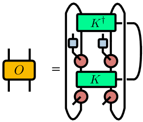
If a quantum channel acts nontrivially on only qubits, it implies that the quasi-stochastic matrix acts also only on qubits. The relation between the quasi-stochastic gates and the local quantum channel in Eq.12 is graphically depicted in Fig.A1 using tensor diagrams.
Appendix B Liouville-Von Neumann Equation in POVM Formulation
In Eq.2 we have discussed how unitary evolution on a quantum state in the traditional density matrix formulation translates into the factorized IC-POVM formulation used in our study. Accordingly, the unitary dynamics induced by Hamiltonian acting on the system during an infinitesimal time , i.e., , implies an equation of motion for the measurement statistics
| (13) |
This is equivalent to the Liouville-Von Neumann equation .
A solution to Eqs.(13) for a time-independet Hamiltonian is given by , where the matrix elements .
Appendix C Linblad Equation in POVM Formulation
Applicable to open quantum systems, an infinitesimal Markovian but non-unitary evolution leads to the equivalent of the Linblad equation
| (14) |
where the matrix elements are augmented to
| (15) |
Here, the operators are called Lindblad operators or quantum jump operators. Like the Liouville-Von Neumann equation, Eq.(15) has a solution for a time-independet Hamiltonians given by .
Appendix D Measurements
Although the probabilistic representation of the quantum state in Eq.1 already provides the measurement statistics of the factorized POVM , the statistics of other POVMs , e.g. a POVM describing standard measurements in the computational basis and other experimentally relevant operators, are related to via the Born rule:
where can be characterized as a quasi-conditional probability distribution since its entries can either be positive or negative but its trace over is the identity . Due to its evocative resemblance with the law of total probability, the relation between measurement statistics and is often called the quantum law of total probability in quantum Bayesianism.Fuchs and Schack (2013)
Appendix E Qplex and positivity of quantum states
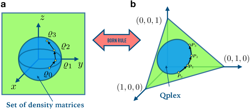
The traditional quantum theory can be viewed as a noncommutative generalization of probability theory where quantum states are specified by Hermitian, positive semi-definite trace one matrices. However, quantum states can also be specified through probability distributions corresponding to the statistics of the outcome of an informationally complete physical measurement. From this viewpoint, quantum theory is not necessarily a generalization of probability theory; instead, it can be seen as augmenting probability theory with further rules for dynamics and measurements on quantum systems.Appleby et al. (2017) When we represent the probabilities of a IC-POVM as points in the corresponding probability simplex , these probabilities are not arbitrary, since not any point of the simplex can represent a quantum state, only a subset of the simplex. For a symmetric IC-POVM,Renes et al. (2004) this subset is referred to as the Qplex.Appleby et al. (2017) Even though the IC-POVM used in our work is not symmetric, we will still refer to the subset of distributions with a corresponding quantum state in Eq.1 as a Qplex. The space of all possible states of a given quantum system and the corresponding Qplex are schematically represented in Fig.A2(a)-(b).
A small quantum computation in also depicted schematically in Fig.A2(a) and (b). This computation starts with a simple pure product state followed by the application of three unitary matrices which take the state from to . These computations occur at the boundary separating valid quantum states from other operators; such boundary includes all the pure states. Correspondingly, since the relation between the space of quantum states and the Qplex is linear (i.e. the Born rule), quantum computations in the probabilistic language take place at the edges of the Qplex, as illustrated in Fig.A2(b).
While these observations do not have any major conceptual implication for the physical realization of quantum computations, this geometric interpretation can help us clarify some aspects we observe in the results from our simulation strategy. The most important aspect is the fact that the probabilistic model in our study, in general, lives in an standard simplex and is not constrained to the subset of valid “quantum” distributions. Even though the update rule in Eq.2 should produce distributions that live on the Qplex, since we use an approximate update, it is possible that the model may temporarily leave the Qplex. This is observed in Fig.4(d) and (h) where we observe values of quantum fidelity higher than 1, which means that during the training process, the ransformer induces matrices in Eq.1 that are not valid quantum states. Note that the fidelity in Fig.4(d) and (h) eventually converges and stays at values very close to one and that the oscillations above 1 disappear, suggesting that the state is getting closer and closer to the target, valid quantum state.
Appendix F Variational Circuit for TFIM
We use the variational circuit depicted in Fig.A3 for the 6-qubit TFIM preparation.Ho and Hsieh (2019) The parameters for gamma and beta are taken alternatively from the following sequence describing a circuit with 4 layers, . Note that in our simulations, we do not directly transform the original gates into quasi-stochastic gates. To save computational resources, we combine the quantum gates encircled in rounded blue squares, after which we transform them into quasi-stochastic matrices.
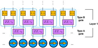
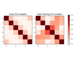
Using this circuit, we have also computed the correlation of the exact variational circuit in Fig.A3 and the POVM trained circuit, which are compared in Fig. A4.
Appendix G Supplementary Figures
References
- Feynman (1982) R. P. Feynman, International Journal of Theoretical Physics 21, 467 (1982).
- Domb (2000) C. Domb, Phase Transitions and Critical Phenomena, Phase Transitions and Critical Phenomena No. v. 19 (Elsevier Science, 2000).
- Ferrie (2011) C. Ferrie, Reports on Progress in Physics 74, 116001 (2011).
- Veitch et al. (2012) V. Veitch, C. Ferrie, D. Gross, and J. Emerson, New Journal of Physics 14, 113011 (2012).
- Raussendorf et al. (2019) R. Raussendorf, J. Bermejo-Vega, E. Tyhurst, C. Okay, and M. Zurel, arXiv:1905.05374 [quant-ph] (2019), arXiv:1905.05374 [quant-ph] .
- Fuchs and Schack (2011) C. A. Fuchs and R. Schack, Foundations of Physics 41, 345 (2011).
- Chruściński et al. (2015) D. Chruściński, V. I. Man’ko, G. Marmo, and F. Ventriglia, Physica Scripta 90, 115202 (2015).
- van de Wetering (2018) J. van de Wetering, Electronic Proceedings in Theoretical Computer Science 266, 179 (2018), arXiv:1704.08525 .
- Carrasquilla et al. (2019) J. Carrasquilla, G. Torlai, R. G. Melko, and L. Aolita, Nature Machine Intelligence 1, 155 (2019).
- Kiktenko et al. (2019) E. O. Kiktenko, A. O. Malyshev, A. S. Mastiukova, V. I. Man’ko, A. K. Fedorov, and D. Chruściński, arXiv:1908.03404 [quant-ph] (2019), arXiv:1908.03404 [quant-ph] .
- Nielsen and Chuang (2011) M. A. Nielsen and I. L. Chuang, Quantum Computation and Quantum Information: 10th Anniversary Edition, 10th ed. (Cambridge University Press, New York, NY, USA, 2011).
- Bouland et al. (2018) A. Bouland, B. Fefferman, C. Nirkhe, and U. Vazirani, (2018), arXiv:1803.04402 [quant-ph] .
- De Raedt et al. (2007) K. De Raedt, K. Michielsen, H. De Raedt, B. Trieu, G. Arnold, M. Richter, T. Lippert, H. Watanabe, and N. Ito, Computer Physics Communications 176, 121 (2007).
- Markov and Shi (2008) I. Markov and Y. Shi, SIAM Journal on Computing 38, 963 (2008).
- Smelyanskiy et al. (2016) M. Smelyanskiy, N. P. D. Sawaya, and A. Aspuru-Guzik, arXiv:1601.07195 [quant-ph] (2016), arXiv:1601.07195 [quant-ph] .
- Pednault et al. (2017) E. Pednault, J. A. Gunnels, G. Nannicini, L. Horesh, T. Magerlein, E. Solomonik, E. W. Draeger, E. T. Holland, and R. Wisnieff, arXiv:1710.05867 [quant-ph] (2017), arXiv:1710.05867 [quant-ph] .
- Chen et al. (2018) J. Chen, F. Zhang, C. Huang, M. Newman, and Y. Shi, arXiv:1805.01450 [quant-ph] (2018), arXiv:1805.01450 [quant-ph] .
- Markov et al. (2018) I. L. Markov, A. Fatima, S. V. Isakov, and S. Boixo, arXiv:1807.10749 [quant-ph] (2018), arXiv:1807.10749 [quant-ph] .
- Li et al. (2018) R. Li, B. Wu, M. Ying, X. Sun, and G. Yang, arXiv:1804.04797 [quant-ph] (2018), arXiv:1804.04797 [quant-ph] .
- Jónsson et al. (2018) B. Jónsson, B. Bauer, and G. Carleo, arXiv:1808.05232 [cond-mat, physics:physics, physics:quant-ph] (2018), arXiv:1808.05232 [cond-mat, physics:physics, physics:quant-ph] .
- Penrose (1971) R. Penrose, Combinatorial mathematics and its applications 1, 221 (1971).
- Ćurgus and Jewett (2007) B. Ćurgus and R. I. Jewett, arXiv:0709.0309 [math] (2007), arXiv:0709.0309 [math] .
- Ćurgus and Jewett (2015) B. Ćurgus and R. I. Jewett, The American Mathematical Monthly 122, 36 (2015).
- Kingma and Ba (2015) D. P. Kingma and J. Ba, in 3rd International Conference on Learning Representations, ICLR 2015, San Diego, CA, USA, May 7-9, 2015, Conference Track Proceedings (2015).
- Assaraf and Caffarel (1999) R. Assaraf and M. Caffarel, Phys. Rev. Lett. 83, 4682 (1999).
- He et al. (2015) K. He, X. Zhang, S. Ren, and J. Sun, arXiv:1512.03385 [cs] (2015), arXiv:1512.03385 [cs] .
- Ba et al. (2016) J. L. Ba, J. R. Kiros, and G. E. Hinton, arXiv:1607.06450 [cs, stat] (2016), arXiv:1607.06450 [cs, stat] .
- Luchnikov et al. (2019) I. A. Luchnikov, A. Ryzhov, P.-J. Stas, S. N. Filippov, and H. Ouerdane, Entropy 21, 1091 (2019).
- Vaswani et al. (2017) A. Vaswani, N. Shazeer, N. Parmar, J. Uszkoreit, L. Jones, A. N. Gomez, L. u. Kaiser, and I. Polosukhin, in Advances in Neural Information Processing Systems 30, edited by I. Guyon, U. V. Luxburg, S. Bengio, H. Wallach, R. Fergus, S. Vishwanathan, and R. Garnett (Curran Associates, Inc., 2017) pp. 5998–6008.
- Becca and Sorella (2017) F. Becca and S. Sorella, Quantum Monte Carlo Approaches for Correlated Systems (Cambridge University Press, 2017).
- Shen (2019) H. Shen, arXiv:1905.04271 [cond-mat, stat] (2019), arXiv:1905.04271 [cond-mat, stat] .
- Goodfellow et al. (2016) I. Goodfellow, Y. Bengio, and A. Courville, Deep Learning (MIT Press, 2016) http://www.deeplearningbook.org.
- Paszke et al. (2017) A. Paszke, S. Gross, S. Chintala, G. Chanan, E. Yang, Z. DeVito, Z. Lin, A. Desmaison, L. Antiga, and A. Lerer, in NIPS Autodiff Workshop (2017).
- Ho and Hsieh (2019) W. W. Ho and T. H. Hsieh, SciPost Phys. 6, 29 (2019).
- Appleby et al. (2017) M. Appleby, C. A. Fuchs, B. C. Stacey, and H. Zhu, The European Physical Journal D 71, 197 (2017).
- Peruzzo et al. (2014) A. Peruzzo, J. McClean, P. Shadbolt, M.-H. Yung, X.-Q. Zhou, P. J. Love, A. Aspuru-Guzik, and J. L. O’Brien, Nature Communications 5, 1 (2014).
- Fuchs et al. (2017) C. A. Fuchs, M. C. Hoang, and B. C. Stacey, Axioms 6, 21 (2017), arXiv:1703.07901 .
- Cerf and Koonin (1998) N. J. Cerf and S. E. Koonin, Mathematics and Computers in Simulation 47, 143 (1998).
- Mari and Eisert (2012) A. Mari and J. Eisert, Phys. Rev. Lett. 109, 230503 (2012).
- Parmar et al. (2018) N. Parmar, A. Vaswani, J. Uszkoreit, Ł. Kaiser, N. Shazeer, A. Ku, and D. Tran, arXiv:1802.05751 [cs] (2018), arXiv:1802.05751 [cs] .
- Kraus (1983) K. Kraus, States, Effects, and Operations: Fundamental Notions of Quantum Theory, edited by A. Böhm, J. D. Dollard, and W. H. Wootters, Lecture Notes in Physics (Springer-Verlag, Berlin Heidelberg, 1983).
- Fuchs and Schack (2013) C. A. Fuchs and R. Schack, Reviews of Modern Physics 85, 1693 (2013).
- Renes et al. (2004) J. M. Renes, R. Blume-Kohout, A. J. Scott, and C. M. Caves, Journal of Mathematical Physics 45, 2171 (2004).