COMPOSITE FERMIONS
AS DEFORMED OSCILLATORS:
WAVEFUNCTIONS AND ENTANGLEMENT ¹

Abstract

Composite structure of particles somewhat modifies their statistics, compared to the pure Bose- or Fermi-ones.  The spin-statistics theorem, so, is not valid anymore.  Say, $\pi$-mesons, excitons, Cooper pairs are not ideal bosons, and, likewise, baryons are not pure fermions.  In our preceding papers, we studied bipartite composite boson (i.e.  quasiboson) systems via a realization by deformed oscillators.  Therein, the interconstituent entanglement characteristics such as entanglement entropy and purity were found in terms of the parameter of deformation.  Herein, we perform an analogous study of composite Fermi-type particles, and explore them in two major cases: (i) ‘‘boson + fermion’’ composite fermions (or cofermions, or CFs); (ii) ‘‘deformed boson + fermion’’ CFs.  As we show, cofermions in both cases admit only the realization by ordinary fermions.  Case (i) is solved explicitly, and admissible wavefunctions are found along with entanglement measures.  Case (ii) is treated within few modes both for CFs and constituents.  The entanglement entropy and purity of CFs are obtained via the relevant parameters and illustrated graphically.

1 Introduction

Composite fermions play a significant role in modern quantum physics.  Suffice it to mention a few instances of CFs: these include quasiparticles involved in the theory of fractional quantum Hall effect [1]; also, let us mention baryons and pentaquarks as known instances in hadron physics [2,​ 3,​ 4].  In this paper, we will focus on the entanglement properties of composite fermions basing on their fermionic oscillator realization, in two relatively simple cases: cofermion built from a pure fermion and a pure boson, or the cofermion as a composite made of a pure fermion and a deformed boson (taken in general form).

In our preceding works [5,​ 6,​ 7,​ 8], we studied bipartite (two-component) composite ‘‘bosons’’ of two types: ‘‘fermion + fermion’’ and ‘‘boson + boson’’ with creation and annihilation operators within the typical ansatz

$$A^{\dagger}_{\alpha}=\sum\limits_{\mu\nu}\Phi_{\alpha}^{\mu\nu}a^{\dagger}_{\mu}b^{\dagger}_{\nu},\ \quad A_{\alpha}=\sum\limits_{\mu\nu}\overline{\Phi_{\alpha}^{\mu\nu}}b_{\nu}a_{\mu},$$ (1)

where the creation operators $a^{\dagger}_{\mu}$, $b^{\dagger}_{\nu}$ for the (distinguishable) constituents taken either both fermionic or both bosonic.  In [5,​ 6], it was shown that composite bosons of a particular form (with appropriate wavefunctions $\Phi_{\alpha}^{\mu\nu}$) can be realized, in the operator sense, by suitable deformed bosons (deformed oscillators).

An important concept in quantum information theory, quantum communication, and teleportation [9,​ 10] is the notion of entanglement or quantum correlation between the constituents of a composite particle or composite system.  Recently, this concept was actively studied just in the context of composite bosons [11,​ 12,​ 7,​ 13].  Among the measures characterizing the degree of entanglement, best known are the entanglement entropy and purity (= inverse of the Schmidt number) [9,​ 10].  The measures of intercomponent entanglement in a quasiboson quantify to what extent the properties of a quasiboson approach those of a true boson [11,​ 12,​ 15,​ 14].

For composite bosons realizable by deformed quantum oscillators, it is possible to directly link [7] the relevant parameter of deformation with the entanglement characteristics of a composite boson.  Then the characteristics (or measures) of bipartite entanglement with respect to $a$- and $b$-subsystems, see (1), can be found explicitly [7] in terms of the deformation parameter: for a single composite boson, for multi-quasiboson states, and for coherent states constructed for such quasibosons.

As a very important issue, the influence of system’s energy on quantum correlation and/or quantum statistics properties of the system was studied, for the quasibosons, in [8].  The energy of the quasiboson differs from the energy of a respective ideal boson, and the difference (including the energy of bound states) essentially depends [8] on the quasiboson’s entanglement, clearly showing a deviation from the bosonic behavior.  Such entanglement-energy relation is relevant to quantum information research, quantum communication, entanglement production [16], quantum dissociation processes [17], particle addition or subtraction [18,​ 19], etc.

Below, we explore the cofermions.  Since the entanglement entropy is of primary interest, after the appropriate analysis of the realization issue, we find the entanglement entropy $S_{\mathrm{ent}}$ characterizing the composite fermion.  Our treatment is performed for one-CF states (to compare, the respective results for one quasiboson states are also briefly sketched).  In some analogy with the case of composite bosons, we take the cofermions as bipartite systems realized by mode-independent  fermionic oscillators.  Another entanglement measure, purity, is considered in a special case.

We have to emphasize that our investigation of entanglement concerns not a many-cofermion system, but the states of a single (or isolated) cofermion.  Accordingly, the considered entanglement and its entropy concern two constituents of the bipartite CF. These features make our approach and analysis essentially different from some recent works on the entanglement entropy of a system of free or composite fermions, see, e.g., [20,​ 21], where the spatial size of a subsystem plays the basic role, and entanglement entropy was viewed in a way different from our one.

In Sec. 2, a sketch of the realized composite bosons is given.  Sections 3–5 deal with cofermions: we perform the analysis of operator-level realization of cofermions by (deformed) fermionic oscillators.  Then the entanglement entropy of the CF one-particle states is explored.  Modified CFs (composed of fermion and deformed boson) are analyzed in Sec. 5(b).  The purity for a CF state is considered in Sec. 5(a).  The paper ends with conclusions.

2 Quasibosons Formed
as Two-Fermion (Two-Boson) Composites [5]

Recall the main facts about composite bosons realized [6,​ 5] by a set of independent modes of deformed bosons (deformed oscillators), given by the defining deformation structure function $\varphi(n)$ [22].  At the algebraic level, the quasiboson operators $A_{\alpha}$, $A^{\dagger}_{\alpha}$ and the number operator $N_{\alpha}$ satisfy the same relations on the states as the corresponding deformed oscillator creation/annihilation and number operators:

$$A^{\dagger}_{\alpha}A_{\alpha}\!\simeq\!\varphi(N_{\alpha}),\leavevmode\nobreak\ \leavevmode\nobreak\ \leavevmode\nobreak\ [A_{\alpha},A^{\dagger}_{\beta}]\!\simeq\!\delta_{\alpha\beta}\bigl{(}\varphi(N_{\alpha}\!+\!1)\!-\!\varphi(N_{\alpha})\bigr{)},$$

$$[N_{\alpha},A^{\dagger}_{\beta}]\simeq\delta_{\alpha\beta}A^{\dagger}_{\beta},\quad[N_{\alpha},A_{\beta}]\simeq-\delta_{\alpha\beta}A_{\beta}.$$

Here, $\simeq$ denotes weak equality (i.e. on the states), symbols $\delta_{\alpha\beta}$ reflect mode independence.  In such realization, the structure function $\varphi(n)$ involves [6,​ 5] the discrete deformation parameter $f$ and is quadratic in the quasiparticles number $n$  ($\kappa=+1$ or $-1$ for two bosonic or two fermionic constituents):

$$\varphi(n)=\Biggl{(}\!1+\kappa\frac{f}{2}\!\Biggr{)}n-\kappa\frac{f}{2}n^{2},\quad f=\frac{2}{m},$$ (2)

$m=1,2,...$ . The matrices $\Phi_{\alpha}$ in (1) are [6,​ 5]

$$\Phi_{\alpha}=U_{1}(d_{a})\mathop{\mathrm{diag}}\nolimits\Bigl{\{}0..0,\sqrt{f\!/2}\,U_{\alpha}(m),0..0\Bigr{\}}U^{\dagger}_{2}(d_{b}),\!\!\!$$ (3)

where $U_{j}(r)$ stands for an arbitrary unitary $r\times r$ matrices, the dimension $d_{a}$ or $d_{b}$ is the total number of modes for constituents with operators $a_{\mu}$ or $b_{\nu}$.

Note that the state of one composite boson,

$$|\Psi_{\alpha}\rangle\!=\!\sum\limits_{\mu\nu}\Phi_{\alpha}^{\mu\nu}|\mu\rangle\!\otimes|\nu\rangle,\quad|\mu\rangle\equiv a^{\dagger}_{\mu}|0\rangle,\ \ \ |\nu\rangle\equiv b^{\dagger}_{\nu}|0\rangle,$$

is, in general, bipartite-entangled relative to the states of two constituent fermions (or two bosons). There are well-known measures of entanglement [10,​ 9]: Schmidt rank $s$, Schmidt number $K$ or its inverse – purity, entanglement entropy $S$, and concurrence $C$.  As proven in [7], the (internal) entanglement entropy of one composite boson

$$S_{\rm ent}=\ln(m)=\ln(2/f).$$ (4)

For the multi-quasibosonic states, the respective extended results were also derived, see [7,​ 8].

The other known measure of entanglement [10,​ 9], purity is inverse to the Schmidt number: $P=1/K$. Note that purity was exploited in connection with the issue of entanglement creation using scattering processes [16] (for other contexts, see [18,​ 23]).  For one-quasiboson entangled system, purity is as well linked [7] with the deformation parameter $m=\frac{2}{f}$:

$$P\!=\!\sum\limits_{k}\lambda_{k}^{4}=\frac{1}{m}$$ (5)

and thus takes discrete values.

3 Cofermion – as Fermion
plus Deformed Boson

From now on, we consider composite fermions which are composed of a pure (or deformed) boson and a pure fermion, from the viewpoint of their realization by deformed fermions.  Like for composite bosons, the realization of CFs is required to be constructed in the way that enables to treat CFs’ creation, annihilation, and number operators as the respective operators of deformed fermions.  In turn, this gives the advantages compared to the standard quantum mechanical or macroscopic approach with explicit direct consideration of a composite structure, – to perform calculations, in the effective or approximate description.  CFs’ creation and annihilation operators are given by the same ‘‘ansatz’’ as in (1), but now $a^{{\dagger}}_{\mu},a_{\mu}$ are, respectively, the creation and annihilation operators for the constituent bosons (deformed or not) and $b^{{\dagger}}_{\nu},b_{\nu}$ – those for the constituent fermions, with standard anticommutation relations for the latter.  For simplicity, we suppose that different modes of deformed bosons are independent.  Then we have the following defining commutation relations for the operators of constituent bosons (deformed or not; $n^{a}_{\mu}$ is the particle number operator for deformed bosons in the $\mu$-mode):

$$a^{\dagger}_{\mu}a_{\mu}=\chi(n^{a}_{\mu}),\leavevmode\nobreak\ \leavevmode\nobreak\ \leavevmode\nobreak\ \leavevmode\nobreak\ [a_{\mu},a^{\dagger}_{\mu^{\prime}}]=\delta_{\mu\mu^{\prime}}\bigl{(}\chi(n^{a}_{\mu}\!+\!1)\!-\!\chi(n^{a}_{\mu})\bigr{)};$$

$$[a^{\dagger}_{\mu},a^{\dagger}_{\mu^{\prime}}]=0;\leavevmode\nobreak\ \leavevmode\nobreak\ \leavevmode\nobreak\ [n^{a}_{\mu},a^{\dagger}_{\mu}]=a^{\dagger}_{\mu}.$$

Here, the deformation structure function $\chi(n)$ means the general case of deformed constituent boson.  For a non-deformed, i.e. usual, boson, $\chi(N)\equiv N$.  In the case of deformation, $\chi(N)$ depends on one or more deformation parameters which admit a ‘‘no-deformation’’ limit.  It is convenient to work with deformed boson states normalized as $|\mu\rangle=a^{{\dagger}}_{\mu}|0\rangle$.  The same concerns CF states, obeying the normalization condition for structural matrices (wavefunctions):

$$\mathop{\mathrm{Tr}}\nolimits(\Phi_{\beta}\Phi^{\dagger}_{\alpha})=\delta_{\alpha\beta}.$$ (6)

We suppose CFs to behave themselves on the states as deformed particles with a structure function $\varphi(N)$.  Respective deformed fermions providing the realization are supposed to be independent (in the fermionic sense).  Defining the number operator $N_{\alpha}$ for CFs as $\varphi(N_{\alpha})\simeq A^{\dagger}_{\alpha}A_{\alpha}$, we write the realization conditions:

$$\{A_{\alpha},A^{\dagger}_{\beta}\}\simeq\delta_{\alpha\beta}[\varphi(N_{\alpha}\!+\!1)\!+\!\varphi(N_{\alpha})],$$ (7)

$$\{A^{\dagger}_{\alpha},A^{\dagger}_{\beta}\}\simeq 0,\leavevmode\nobreak\ \leavevmode\nobreak\ \leavevmode\nobreak\ \alpha\neq\beta;\quad[N_{\alpha},A^{\dagger}_{\beta}]\simeq\delta_{\alpha\beta}A^{\dagger}_{\beta}.$$ (8)

The first requirement in (8) holds automatically, and moreover, in the strict sense for all $\alpha$ and $\beta$,

$$\{A^{{\dagger}}_{\alpha},A^{{\dagger}}_{\beta}\}=0,\ \text{particularly}\ (A^{{\dagger}}_{\alpha})^{2}=0.$$ (9)

The latter, fermionic nilpotency, and (7) considered on vacuum and one-CF states, along with the second equation in (8), yield the usual fermionic structure function $\varphi(N)$:

$$\varphi(0)=\varphi(2)=...=0,\quad\varphi(1)=\chi(1)=1.$$ (10)

We analyze requirement (7), proceeding like in [5], but alternate (interchange) the commutator and anticommutator of the l.h.s.  of (7) with $A_{\gamma_{i}}^{\dagger}$.  Introducing the notation

$$\Delta^{\!k}\chi(n^{a}_{\mu})\!\equiv\!\sum\limits_{l=0}^{k}(-1)^{k-l}{k\choose l}\chi(n^{a}_{\mu}\!+\!l),\ \ k\!=\!0,1,...,$$

with the first terms

$$\Delta^{0}\chi(n^{a}_{\mu})=\chi(n^{a}_{\mu}),\quad\Delta^{1}\chi(n^{a}_{\mu})=\chi(n^{a}_{\mu}\!+\!1)-\chi(n^{a}_{\mu}),$$

$$\Delta^{2}\chi(n^{a}_{\mu})=\chi(n^{a}_{\mu}\!+\!2)-2\chi(n^{a}_{\mu}\!+\!1)+\chi(n^{a}_{\mu}),$$

for the anticommutator $\{A_{\alpha},A^{\dagger}_{\beta}\}$ in (7), we have

$$\{A_{\alpha},A_{\beta}^{\dagger}\}=\sum\limits_{\mu}(\Phi_{\beta}\Phi_{\alpha}^{\dagger})^{\mu\mu}\Delta^{1}\chi(n^{a}_{\mu})\,+$$

$$+\sum_{\mu\mu^{\prime}}(\Phi_{\beta}\Phi_{\alpha}^{\dagger})^{\mu^{\prime}\mu}a_{\mu^{\prime}}^{\dagger}a_{\mu}-\sum_{\mu\nu\nu^{\prime}}\overline{\Phi_{\alpha}^{\mu\nu}}\Phi_{\beta}^{\mu\nu^{\prime}}\!\Delta^{1}\chi(n^{a}_{\mu})\,b_{\nu^{\prime}}^{\dagger}b_{\nu}.$$

This will be exploited below.  For a nondeformed constituent boson ($\chi(n)\equiv n$), the latter with the use of (6) reduces to

$$\bigl{\{}\!A_{\alpha},\!A_{\beta}^{\dagger}\!\bigr{\}}\!=\!\delta_{\alpha\beta}+\!\sum_{\mu\mu^{\prime}}\!(\Phi_{\beta}\Phi^{\dagger}_{\alpha})^{\mu^{\prime}\!\mu}a^{\dagger}_{\mu^{\prime}}a_{\mu}-\!\sum_{\nu\nu^{\prime}}\!(\Phi_{\alpha}^{\dagger}\!\Phi_{\beta})^{\nu\nu^{\prime}}\!b^{\dagger}_{\nu^{\prime}}b_{\nu}.$$

Next, we calculate the commutator

$$\bigl{[}\{A_{\alpha},A^{\dagger}_{\beta}\},A^{\dagger}_{\gamma}\bigr{]}\!=\!\!\sum\limits_{\mu\mu_{1}\!\nu_{1}}\!\!\Bigl{[}(\Phi_{\beta}\Phi^{\dagger}_{\alpha})^{\mu_{1}\mu}\Phi^{\mu\nu_{1}}_{\gamma}\,-$$

$$-\,(\Phi_{\gamma}\Phi^{\dagger}_{\alpha})^{\mu_{1}\mu}\Phi^{\mu\nu_{1}}_{\beta}\Bigr{]}a^{\dagger}_{\mu_{1}}b^{{\dagger}}_{\nu_{1}}\cdot\bigl{(}\Delta^{1}\chi(n^{a}_{\mu})+\delta_{\mu\mu_{1}}\Delta^{2}\chi(n^{a}_{\mu})\bigr{)}\,+$$

$$+\sum\limits_{\mu\nu\nu_{1}\!\nu_{2}}\overline{\Phi_{\alpha}^{\mu\nu}}\Phi_{\beta}^{\mu\nu_{1}}\Phi_{\gamma}^{\mu\nu_{2}}a^{\dagger}_{\mu}b^{\dagger}_{\nu_{1}}\Delta^{2}\chi(n^{a}_{\mu})b^{\dagger}_{\nu_{2}}b_{\nu}.$$ (11)

A nondeformed analog (at $\chi(n)\equiv n$) of the latter is

$$[\{A_{\alpha},A^{\dagger}_{\beta}\},A^{\dagger}_{\gamma}]=\sum_{\mu\nu}\bigl{(}\Phi_{\beta}\Phi^{\dagger}_{\alpha}\Phi_{\gamma}-\Phi_{\gamma}\Phi^{\dagger}_{\alpha}\Phi_{\beta}\bigr{)}^{\mu\nu}a^{\dagger}_{\mu}b^{\dagger}_{\nu}.$$

So, the validity of (7) on one-CF states $|\gamma\rangle$ yields the following relation of basic importance for the wavefunctions:

$$(\Phi_{\beta}\Phi^{\dagger}_{\alpha}\Phi_{\gamma})^{\mu\nu}-(\Phi_{\gamma}\Phi^{\dagger}_{\alpha}\Phi_{\beta})^{\mu\nu}\,+$$

$$+\,\bigl{(}\chi(2)\!-2\bigr{)}\bigl{[}(\Phi_{\beta}\Phi^{\dagger}_{\alpha})^{\mu\mu}\Phi_{\gamma}^{\mu\nu}\!\!-\!(\Phi_{\gamma}\Phi^{\dagger}_{\alpha})^{\mu\mu}\Phi^{\mu\nu}_{\beta}\bigr{]}\!=0.\,$$ (12)

Note that, in the case of non-deformed constituent boson, this relation yields $[\{A_{\alpha},A^{\dagger}_{\beta}\},A^{\dagger}_{\gamma}]=0$.  That leads to a closed set of realization conditions on the matrices $\Phi_{\alpha}$, see (6),(7), namely:

$$\Phi_{\beta}\Phi^{\dagger}_{\alpha}\Phi_{\gamma}-\Phi_{\gamma}\Phi^{\dagger}_{\alpha}\Phi_{\beta}=0,\quad\mathop{\mathrm{Tr}}\nolimits(\Phi_{\beta}\Phi^{\dagger}_{\alpha})=\delta_{\alpha\beta}.$$ (13)

However, for a nontrivial deformation, i.e.  $\chi(N)\not\equiv N$, the double and higher commutators (or anticommutators) are significant and must be taken into account (we drop them).

4 Composite Quasifermions
with Non-Deformed Constituent Boson

Consider the realization of CFs formed of a usual boson and a fermion.  The respective wavefunctions of CFs realized by usual fermions satisfy Eqs. (13) which will be solved below.  Let us choose a matrix $\Phi_{\alpha}=\Phi_{\alpha_{1}}$ with maximal rank and perform the singular value (SVD- or Schmidt-) decomposition:

$$\Phi_{\alpha_{1}}\!=U_{1}D_{\alpha_{1}}V^{\dagger}_{1},\quad$$

$$D_{\alpha_{1}}\!=\mathop{\mathrm{diag}}\nolimits\{\lambda^{\alpha_{1}}_{i}\!,i=\kappa_{1},...,\kappa_{r},...\}=$$

$$=\mathop{\mathrm{diag}}\nolimits\{\lambda^{\alpha_{1}}_{\kappa_{1}}E_{m_{1}},\lambda^{\alpha_{1}}_{\kappa_{2}}E_{m_{2}},...,\lambda^{\alpha_{1}}_{\kappa_{r}}E_{m_{r}}\}$$ (14)

with real non-negative $\lambda^{\alpha_{1}}_{\kappa_{l}}$ put in descending order , $\lambda^{\alpha_{1}}_{\kappa_{1}}\!>\!...\,\,\!>\!\lambda^{\alpha_{1}}_{\kappa_{r}}\!\geq\!0$, obeying $\sum_{l}m_{l}(\lambda^{\alpha_{1}}_{\kappa_{l}})^{2}\!=\!1$, and unitary matrices $U_{1}$, $V_{1}$.  For remaining matrices $\Phi_{\gamma}$, $\gamma\neq\alpha_{1}$, we make replacement $\Phi_{\gamma}\to\tilde{\Phi}_{\gamma}$:

$$\Phi_{\gamma}=U_{1}\tilde{\Phi}_{\gamma}V^{\dagger}_{1},\ \ \ \gamma\neq\alpha_{1}.$$ (15)

The first equation in (13) at $\alpha\!=\!\beta\!=\!\alpha_{1}$ now reads

$$D_{\alpha_{1}}^{2}\tilde{\Phi}_{\gamma}\!-\!\tilde{\Phi}_{\gamma}D_{\alpha_{1}}^{2}\!=\!0\ \ {\rm or}\ \ \bigl{(}(\lambda^{\alpha_{1}}_{i})^{2}\!-\!(\lambda^{\alpha_{1}}_{j})^{2}\bigr{)}(\tilde{\Phi}_{\gamma})_{ij}\!=\!0.$$

If $\lambda^{\alpha_{1}}_{i}\!\neq\!\lambda^{\alpha_{1}}_{j},$ we have $(\tilde{\Phi}_{\gamma})_{ij}\!=\!0$.  According to the block-diagonal form of $D_{\alpha_{1}}$, see (14), the other matrices $\tilde{\Phi}_{\gamma}$ also take block-diagonal form:

$$\tilde{\Phi}_{\gamma}=\mathop{\mathrm{diag}}\nolimits\{\tilde{\Phi}_{\gamma,1},\tilde{\Phi}_{\gamma,2},...,\tilde{\Phi}_{\gamma,r}\},\ \ \gamma\neq\alpha_{1}.$$

The dimensions of unit matrices $E_{m_{k}}$ and square matrices $\tilde{\Phi}_{\alpha,k}$ are equal to the multiplicities of singular values $\lambda^{\alpha_{1}}_{\kappa_{k}}$.  Now, the first equation in (13) reduces to the set of $r$ independent systems, $k=1,2,..,r$:

$$\lambda^{\alpha_{1}}_{\kappa_{k}}(\tilde{\Phi}^{\dagger}_{\beta,k}\tilde{\Phi}_{\gamma,k}-\tilde{\Phi}_{\gamma,k}\tilde{\Phi}^{\dagger}_{\beta,k})=0,$$ (16)

$$\lambda^{\alpha_{1}}_{\kappa_{k}}(\tilde{\Phi}_{\beta,k}\tilde{\Phi}_{\gamma,k}-\tilde{\Phi}_{\gamma,k}\tilde{\Phi}_{\beta,k})=0,$$ (17)

$$\tilde{\Phi}_{\beta,k}\tilde{\Phi}^{\dagger}_{\alpha,k}\tilde{\Phi}_{\gamma,k}\!-\!\tilde{\Phi}_{\gamma,k}\tilde{\Phi}^{\dagger}_{\alpha,k}\tilde{\Phi}_{\beta,k}=0,\ \ \alpha,\!\beta,\!\gamma\!\neq\!\alpha_{1}.$$ (18)

From (16)–(17), we infer that the matrices $\tilde{\Phi}_{\gamma,k}$, $\gamma\neq$ $\neq\alpha_{1}$, constitute the set of commuting normal matrices (commuting with their Hermitian conjugate ones) at fixed $k=1,2,..,r-1$ and possibly at fixed $k=r$, if $\lambda^{\alpha_{1}}_{\kappa_{r}}\neq 0$.  Under such premises, as known [24], there is a fixed unitary matrix $\tilde{U}_{k}$ such that $\tilde{\Phi}_{\gamma,k}=\tilde{U}_{k}\tilde{D}_{\gamma,k}\tilde{U}_{k}^{\dagger}$ with diagonal one $\tilde{D}_{\gamma,k}$, $\gamma\neq\alpha_{1}$.  If $\lambda^{\alpha_{1}}_{\kappa_{r}}\neq 0,$ Eqs. (18) are automatically satisfied, and we have

$$\Phi_{\alpha}\!=\!UD_{\alpha}V^{\dagger},\ \ D_{\alpha}|\mathop{=}\limits_{\alpha\neq\alpha_{1}}\mathop{\mathrm{diag}}\nolimits\{\tilde{D}_{\alpha,1},...,\tilde{D}_{\alpha,r}\}$$ (19)

with $U\!=\!U_{1}\mathop{\mathrm{diag}}\nolimits\{\tilde{U}_{k}\}$, $V\!=\!V_{1}\mathop{\mathrm{diag}}\nolimits\{\tilde{U}_{k}\}$, $k\!=\!\overline{1,r}$.

If $\lambda^{\alpha_{1}}_{\kappa_{r}}=0,$ Eqs. (18) at $k=\overline{1,r\!-\!1}$ are satisfied, while the remaining one, at $k=r$, for $\tilde{\Phi}_{\alpha,r}$, $\alpha\neq\alpha_{1}$, can be solved like above for $\Phi_{\alpha}$.  Thus, by induction on the number $\#\alpha\equiv m_{CF}$ of matrices (modes) $\Phi_{\alpha},$ we can show that (19) with arbitrary $U$ and $V$ presents the general solution of (13) .

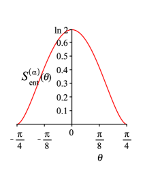
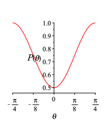
a                                   b

Fig. 1.: Entanglement entropy $S_{\rm ent}^{(\alpha)}$ ($a$) and purity $P$ versus the parameter $\theta$ ($b$) for each mode $\alpha=1,2$

Conversely: all the matrices (19) with $\mathop{\mathrm{Tr}}\nolimits(D_{\beta}\overline{D_{\alpha}})=$ $=\delta_{\alpha\beta}$ satisfy system (13) and thus give its general solution. The diagonal elements of $D_{\alpha}$ are components of the orthonormal vectors $\lambda^{\alpha}$ in the complex space:

$$D_{\alpha}\!\!=\!\mathop{\mathrm{diag}}\nolimits\{\lambda^{\alpha}_{1}\!,\lambda^{\alpha}_{2}\!,...\},\ \ (\lambda^{\alpha}\!\!,\!\lambda^{\beta})\!\equiv\!\sum\limits_{i}\!\!\lambda^{\alpha}_{i}\overline{\lambda^{\beta}_{i}}\!=\!\delta_{\alpha\beta}.\!\!$$ (20)

So, the ‘‘boson-fermion’’ entanglement entropy for realized CFs in the $\alpha$th mode is given along with the orthogonality constraint as

$$S_{\rm entang}^{(\alpha)}\!=\!-\sum\limits_{i}|\lambda^{\alpha}_{i}|^{2}\ln|\lambda^{\alpha}_{i}|^{2},\ \ (\lambda^{\alpha}\!,\!\lambda^{\beta})=\delta_{\alpha\beta}.$$ (21)

Note that, for a parametrization of solution (19), the one of suitable $SU(n)$ can be used: this concerns unitary matrices $U$, $V$ and diagonal matrices $D_{\alpha}$, since their elements $(\lambda^{\alpha}_{i})$ constitute rows (columns) of a unitary matrix, see (20).

Remark 1.  While for the realized composite bosons, the block $U_{\alpha}(m)$ in (3) is associated with the $\alpha$th mode, yielding $m^{2}\!-\!1$ free real parameters in wavefunctions (maximally, $m^{2}/2$-dimensional complex space of states), the realized CFs admit more general wavefunctions.  Indeed, the particular orthonormal CF wavefunctions

$$\Phi_{\alpha}\!=\!U\mathop{\mathrm{diag}}\nolimits\Bigl{\{}0..0,\underbrace{U_{\alpha}(m)D^{(\alpha)}_{m}V_{\alpha}^{\dagger}(m)}_{GL(m)},0..0\Bigr{\}}V^{\dagger}$$

already have avg. $m^{2}\!-\!1$ free complex parameters per mode.

5 Cofermions in Low-Mode Cases

Consider, in more details, low-mode subcases with CFs in two modes $\alpha=1,\,2$, and constituents – upto three modes.  Recall that the general solution in the case of nondeformed constituent boson was given in Sec. 4.

5(a). Two or three modes
of a constituent fermion $+$ usual boson

First, let both constituents be in two modes, i.e. $\mu,\nu=\overline{1,2}$.  The solution for realized wavefunctions reads

$$\Phi_{\alpha}\!=e^{-i\tilde{\alpha}\psi}U\!\left(\!\!\begin{array}[]{cc}\cos(\tilde{\alpha}\!+\!\theta)e^{i\phi}\!\!&\!0\\ 0\!&\!\!\sin(\tilde{\alpha}\!+\!\theta)e^{-i\phi}\end{array}\!\right)\!V^{\dagger},$$ (22)

where $\tilde{\alpha}=\frac{\pi}{2}(\alpha-\alpha_{c})=\mp{\pi\over 4}$, $\alpha_{c}=3/2$.  Due to a low dimensionality of matrices, it is convenient to use the angle parametrization of $SU(2)$.  There can be other parametrization as well.

The entanglement entropy within the CF, realized by a usual fermion, for each of the two modes is as follows:

$$S_{\rm ent}^{(\alpha)}\!\equiv\!-\sum\nolimits_{k}(\lambda^{\alpha}_{k})^{2}\ln(\lambda^{\alpha}_{k})^{2}\Bigl{|}_{\alpha=1,2}\!\!=\!S_{2}\Bigl{(}{\pi\over 4}\!+\!\theta\Bigr{)}\!,$$ (23)

where $S_{2}(x)\equiv-\sin^{2}x\ln\sin^{2}x-\cos^{2}x\ln\cos^{2}x$. This result is visualized in Fig. 1, $a$.  The maximum $S_{\rm ent}\!=\!\ln 2$ may correspond to the most tightly bound state of a realized CF.  Clearly, $S_{\rm ent}=0$ means the opposite, i.e.  the most loosely bound one.  Another entanglement measure of a CF state, purity $P,$ is

$$P|_{\alpha=1,2}\!\equiv\!\sum\nolimits_{k}\!(\lambda^{\alpha}_{k})^{4}\!=\!\frac{1}{4}(3-\cos 4\theta).$$

The purity ranges from $P=1/2$ (at $\theta=0$) to $P=1$ (at $\theta=\pm\frac{\pi}{4}$), see Fig. 1 $b$.

Remark 2.  Nonseparable CF states with fixed intermediate ($0<S_{\rm ent}<\ln 2$) entanglement entropy and two respective wavefunctions $\Phi_{\alpha}^{\mu\nu}$ are parametrized, in total, by 6 independent real parameters.

Non-deformed constituents in three modes

In this case, we take $\alpha=\overline{1,2}$, $\mu,\nu=\overline{1,3}$ so that $\Phi_{\alpha}^{\mu\nu}$ are some $3\times 3$-matrices.  The general solution (19) reads

$$\Phi_{\alpha}=e^{-i\psi(\alpha)}\,U\mathop{\mathrm{diag}}\nolimits\{\lambda^{\alpha}_{1},\lambda^{\alpha}_{2},\lambda^{\alpha}_{3}\}V^{\dagger},\quad U,V\in SU(3),$$

with complex $\lambda^{\alpha}_{k}$, $k=\overline{1,3}$, satisfying the orthonormality conditions (20), and $U,V$ not depending on $\alpha$.

A parametrization of two orthonormal vectors $(\lambda^{1}_{k})$ and $(\lambda^{2}_{k})$ follows from the one of $SU(3)$, since the rows/colums of matrices from $SU(3)$ separately form orthonormal vectors.  Indeed, using the parametrization from [25], we obtain ($\alpha\!=\!1\leftrightarrow\alpha=2$) symmetric unified expressions:

$$(\lambda^{\alpha}_{k})=$$

$$=\!\!\left(\!\begin{aligned} &e^{i\phi_{1}}\!\bigl{(}\sin\theta_{1}\!\cos\theta_{2}\!\cos(\tilde{\alpha}+\theta_{3}\!)\,-\\[-2.84526pt] &-\,\sin\theta_{2}\!\sin(\tilde{\alpha}+\theta_{3}\!)e^{i\phi_{2}}\!\bigr{)},\\ &\cos\theta_{1}\cos(\tilde{\alpha}\!+\!\theta_{3}),\\ &e^{-i\phi_{3}}\!\bigl{(}\sin\theta_{1}\!\sin\theta_{2}\!\cos(\tilde{\alpha}+\theta_{3}\!)\,+\\[-2.84526pt] &+\,\cos\theta_{2}\!\sin(\tilde{\alpha}\!+\!\theta_{3}\!)e^{i\phi_{2}}\!\bigr{)}\end{aligned}\!\right)\!\!,$$ (24)

where $0\leq\theta_{1},\theta_{2},\theta_{3}\!+\!\pi/4\leq\pi/2$, $0\leq\phi_{1,2,3}\leq 2\pi$. The entanglement entropy $S_{\rm ent}^{(\alpha)}(\theta_{1},\theta_{2},\theta_{3},\phi_{2})$ of a CF in the $\alpha$th mode stems from (21) with ‘‘symmetrized’’ squared absolute values of Schmidt coefficients:

$$\bigl{|}\lambda^{\alpha}_{1,3}\bigr{|}^{2}=\frac{1}{4}(1\!+\!\sin^{2}\theta_{1})\pm\frac{1}{4}\,\frac{\cos^{4}\theta_{1}}{1\!+\!\sin^{2}\theta_{1}}\frac{\sin 2(\theta_{3}^{+}\!-\!\theta_{3}^{-})}{\sin 2(\theta_{3}^{+}\!+\!\theta_{3}^{-})}\,-$$

$$-\,\frac{1}{2}\,\frac{\sin 2\theta_{3}^{\pm}}{\sin 2(\theta_{3}^{+}\!+\!\theta_{3}^{-})}\,\cos^{2}\theta_{1}\cos 2\bigl{(}\theta_{3}\!\mp\!\theta_{3}^{\mp}\!+\!\tilde{\alpha}\bigr{)},$$

$$|\lambda^{\alpha}_{2}|^{2}=\frac{1}{2}(1-\sin^{2}\theta_{1})+\frac{1}{2}\,\cos^{2}\theta_{1}\cos 2(\theta_{3}+\tilde{\alpha}),$$ (25)

where two ‘‘shift’’ angles $\theta_{3}^{\pm}$ replace $\theta_{2},\phi_{2}$, while the upper or lower sign corresponds to the first or, respectively, third Schmidt coefficient.  The transition $(\theta_{2},\phi_{2})\to(\theta_{3}^{-},\theta_{3}^{+})$ is given by the unified formula

$$\operatorname{tg}2\theta_{3}^{\pm}=\pm\frac{2\sin\theta_{1}\operatorname{tg}(\theta_{2}+\frac{\pi}{2}\delta_{\mp 1,1})\cos\phi_{2}}{1-\sin^{2}\theta_{1}\operatorname{tg}^{2}(\theta_{2}+\frac{\pi}{2}\delta_{\mp 1,1})}.$$

Note that the ‘‘shift’’ is counted from the parameter $\theta_{3}$ which has a special role being directly linked with the mode number $\alpha$, see (24).

Remark 3.  Parametrization asymmetric under $(\alpha\!=$ $=1)\leftrightarrow(\alpha=2)$, see [25], of the modes can also play a role. From the physics viewpoint, it is possible, when the realization is applied to a system with ad hoc asymmetry, for example, due to an applied external asymmetric field or like for $s$- vs.  $p$-levels/modes of CF.

Thus, the CF entanglement entropies $S_{\rm ent}^{(1)}$ and $S_{\rm ent}^{(2)}$ are parametrized by three angles and one phase. Unlike the constituents in the two-mode $\mu,\nu=\overline{1,2}$ case where $S_{\rm ent}^{(1)}-S_{\rm ent}^{(2)}=0$ and $0\leq S_{\rm ent}^{(\alpha)}\leq\ln 2$, now, in the $\mu,\nu=\overline{1,3}$ case, we have $|S_{\rm ent}^{(1)}-S_{\rm ent}^{(2)}|\leq\ln 2$, while $0\leq S_{\rm ent}^{(\alpha)}\leq\ln 3$. The limits for above differences impose a restriction on the realizable states. To illustrate the dependences $S_{\rm ent}^{(\alpha)}=S_{\rm ent}^{(\alpha)}(\theta_{1},\theta_{3},\theta_{3}^{\mp})$ at $C_{3}$-symmetric choice $\theta_{3}^{\mp}={\pi\over 3}$, for both modes $\alpha=1,2$, Fig. 2 (upper) shows the equientropic curves versus $\theta_{1}$-, $\theta_{3}$-angles. The somewhat similar behavior, though for the entropy of mixing [26] within a three-level system, was given in the context of the $SU(3)$ parametrization of qutrits (see [26]).

\begin{overpic}[width=216.81pt]{fig3.eps} \put(92.0,22.0){$\theta_{3}$} \put(41.0,66.0){$\theta_{1}$} \put(55.0,25.0){'$\alpha=1$' mode} \put(75.0,28.0){\line(1,1){10.0}} \put(70.0,28.0){\line(1,2){5.0}} \put(66.0,28.0){\line(0,1){15.0}} \put(20.0,25.0){'$\alpha=2$' mode} \put(26.0,28.0){\line(-1,1){10.0}} \put(31.0,28.0){\line(-1,2){5.0}} \put(35.0,28.0){\line(0,1){15.0}} \end{overpic}

\begin{overpic}[width=216.81pt]{fig3b.eps} \put(92.0,27.0){$\theta_{3}$} \put(89.0,87.5){$\alpha=1$} \put(88.0,88.5){\vector(-1,0){4.0}} \put(45.0,71.0){$\alpha=2$} \end{overpic}

Fig. 2.: Upper: Equi-entropic curves ($S_{\rm ent}^{(\alpha)}=\rm const$) versus angles $\theta_{1}$ and $\theta_{3}$, at fixed $\theta_{3}^{\mp}={\pi\over 3}$. Lower: Entanglement entropy $S_{\rm ent}^{(2)}(\theta_{3},\phi_{2})$ for cofermion in $\alpha=2$ mode at fixed entanglement entropy $S_{\rm ent}^{(1)}\!=\!\max\!=\!\ln 3$ for $\alpha=1$ cofermion.

Observe that, at $\theta_{3}^{\pm}={\pi\over 3}$ and $\sin^{2}\theta_{1}=\frac{1}{3},$ the entropy for the $\alpha$th mode acquires a $C_{3}$-cyclically symmetric form:

$$S_{\rm ent}^{(\alpha)}=\sum_{l=-1}^{1}S_{1}\bigg{(}\!\frac{2}{3}\cos^{2}\bigl{(}\theta_{3}+\frac{\pi}{3}l+\tilde{\alpha}\bigr{)}\!\bigg{)}\!,$$ (26)

where $S_{1}(x)\!\equiv\!-x\ln x$.

5(b). CFs composed
of a fermion plus a deformed boson

Consider the two-mode case ($\alpha=1,\,2$) of CF composed of a usual fermion and a $\chi$-deformed boson. The specificity of two modes implies that it is sufficient to consider the realization conditions (7)–(8) on the ground and one-CF states.  Then, for the single non-zero two-CF state $A_{1}^{\dagger}A_{2}^{\dagger}|0\rangle$, the realization conditions will be automatically satisfied.  Denoting $\delta\chi_{2}\equiv\chi(2)\!-\!2$, requirement (12) on respective ‘‘one-CF states’’ reduces to two independent equations:

$$L(\Phi_{1},\Phi_{2})\equiv\Phi_{1}\Phi_{1}^{\dagger}\Phi_{2}-\Phi_{2}\Phi_{1}^{\dagger}\Phi_{1}\,+$$

$$+\,\delta\chi_{2}\bigl{[}\mathop{\mathrm{diag}}\nolimits\{(\Phi_{1}\Phi_{1}^{\dagger})^{\mu\mu}\}\Phi_{2}-\mathop{\mathrm{diag}}\nolimits\{(\Phi_{2}\Phi_{1}^{\dagger})^{\mu\mu}\}\Phi_{1}\bigr{]}=0,$$ (27)

$$-L(\Phi_{2},\Phi_{1})=0.$$ (28)

Using substitution (15), restricting to $\mu,\nu\!=\!1,\,2$, taking

$$U_{1}\!=\!U(u,v)\!\equiv\!\Bigl{(}\!\begin{array}[]{cc}u&v\\ -\overline{v}&\overline{u}\end{array}\!\Bigr{)}\!\in\!SU(2),\leavevmode\nobreak\ |u|^{2}\!+\!|v|^{2}=1,$$

and applying the identity

$$U^{\dagger}\mathop{\mathrm{diag}}\nolimits\{(UXU^{\dagger})^{\mu\mu}\}U=\frac{1}{2}X+\frac{1}{2}RXR,$$

with the Hermitian

$$R=\bigg{(}\!\begin{array}[]{cc}|u|^{2}-|v|^{2}&2\overline{u}v\\ 2u\overline{v}&|v|^{2}-|u|^{2}\end{array}\!\bigg{)}\!,$$

we arrive at the matrix equations

$$\chi(2)\!(D_{1}^{2}\tilde{\Phi}_{2}\!-\!\tilde{\Phi}_{2}D_{1}^{2})\!+\!\delta\chi_{2}R\bigl{(}D_{1}^{2}R\tilde{\Phi}_{2}\!-\!\tilde{\Phi}_{2}D_{1}RD_{1}\bigr{)}\!=\!0,$$ (29)

$$\chi(2)(D_{1}\tilde{\Phi}_{2}^{\dagger}\tilde{\Phi}_{2}-\tilde{\Phi}_{2}\tilde{\Phi}_{2}^{\dagger}D_{1})\,+$$

$$+\,\delta\chi_{2}\bigl{(}RD_{1}\tilde{\Phi}_{2}^{\dagger}R\tilde{\Phi}_{2}-R\tilde{\Phi}_{2}\tilde{\Phi}_{2}^{\dagger}RD_{1}\bigr{)}=0.$$ (30)

In view of three-dimensionality of the space of $\tilde{\Phi}^{\dagger}_{2}$ satisfying the orthogonality condition $\mathop{\mathrm{Tr}}\nolimits(D_{1}\tilde{\Phi}^{\dagger}_{2})=0$, we present them as a linear combination:

$$\tilde{\Phi}_{2}=x_{1}\bigg{(}\!\!\begin{array}[]{cc}\lambda^{(1)}_{2}&0\\ 0&-\lambda^{(1)}_{1}\end{array}\!\!\bigg{)}+x_{2}\bigg{(}\!\!\begin{array}[]{cc}0&\varkappa\lambda^{(1)}_{1}\\ \overline{\varkappa}\lambda^{(1)}_{2}&0\end{array}\!\!\bigg{)}\,+$$

$$+\,x_{3}\bigg{(}\!\!\begin{array}[]{cc}0&-\varkappa\lambda^{(1)}_{2}\\ \overline{\varkappa}\lambda^{(1)}_{1}&0\end{array}\!\!\bigg{)}\!,$$

where $\varkappa\!=\!e^{i(\arg v-\arg u)}$.  Equation (30) reduces to three linear (in $x_{1},x_{2},x_{3}$) equations, the associated determinant should be zero:

$$\det\bigl{(}...\bigr{)}=-\chi(2)(\chi(2)-2)|u|^{2}|v|^{2}\bigl{(}|\lambda^{1}_{1}|^{2}\!-|\lambda^{1}_{2}|^{2}\bigr{)}^{2}=0.$$

This is possible in the following cases:

a) $\chi(2)=0$. The solution of (27)–(28) reads

$$\Phi_{\alpha}\!=U(u,(-1)^{\alpha-\!1}v)\!\left(\!\!\begin{array}[]{cc}\cos(\tilde{\alpha}+\theta)\!\!&\!0\\ 0\!&\!\!\sin(\tilde{\alpha}+\theta)\end{array}\!\!\right)\!V^{\dagger}.$$ (31)

b) $\chi(2)=1$. We find two classes of solutions:

$$\Phi_{\alpha}\!=\!\mathop{\mathrm{diag}}\nolimits\bigl{\{}\cos(\tilde{\alpha}+\theta),\sin(\tilde{\alpha}+\theta)\bigr{\}}V^{\dagger},$$ (32)

$$\Phi_{\alpha}\!\equiv\!(\Phi_{\alpha}^{\mu\nu})=\Bigl{(}\delta_{\mu\mu_{0}}\overline{V_{\nu\alpha}\!}\Bigr{)}\!,\leavevmode\nobreak\ \leavevmode\nobreak\ \leavevmode\nobreak\ {\mathrm{fixed}}\leavevmode\nobreak\ \leavevmode\nobreak\ \mu_{0}=1\leavevmode\nobreak\ {\mathrm{or}}\leavevmode\nobreak\ 2.$$ (33)

c) $\chi(2)=2,$ i.e. $\delta\chi_{2}=0$ – non-deformed one, see (22).

d) At $\chi(2)\neq 0,1,2$, the solution is identical to (32).

So, the entanglement entropy of the cofermion containing a deformed boson is either given by the general parameter-dependent expression, see (23), or the constant $S_{\rm ent}=0$ in the special case $\chi(2)=1$, for (33).  The deformations $\chi(2)=0$, $1,$ or $2$ are disjoint from the continuous set.  How the deformation parameter $\chi(2)$ is reflected in physical quantities will be analyzed in the subsequent paper.

6 Conclusions

After we settled the problem of realization of composite fermions (CFs) by usual fermions, we explored the bipartite entanglement (inside the CF) measured by the entanglement entropy of CF.  The analysis has been performed in relatively simpler cases: i) CFs with a non-deformed constituent boson, for which we have considered the examples of two and three modes for the both constituents, ii) CF containing a deformed boson, both in two modes.  The resulting expressions are given in (21) in the case of non-deformed constituents, (23) for CFs and constituents being in two modes, and finally by (24), (26) for two-mode CFs with three-mode constituents.

As is found, for the entanglement entropy of realized CFs of the type ‘‘fermion + deformed boson’’, the constituent boson deformation does not manifest itself in the explicit formulas for the entanglement entropy and purity of CF within each fixed subcase in these one- and two-mode cases.  At first sight, this is in some contrast to the earlier studied entanglement entropy of quasibosons [7], where the major issue was just the dependence on the deformation parameter $f$.  Therein, all other parameters of the states [like those from $U_{1}(d_{a})$, $U_{2}(d_{b})$, $U_{\alpha}(m)$ in (3)] did not enter the entanglement measures.  In the present case of CFs, the situation is different: the CFs are realized by nondeformed fermions, so, the analogous deformation parameter corresponding to CF as a whole is absent.  The quantity $\chi(2),$ being related to the deformation parameter(s), in the case of CF has different origin, since it concerns the constituent of CF.  Nevertheless, there appear additional parameters present in the matrix $\Phi$ of ansatz (1) which, along with $\chi(2)$, define the entanglement entropy of CFs. Thus, these parameters determine the form of CF states (their wavefunctions).  This dependence on the involved parameter is shown in Fig. 1.  Also noteworthy are the properties of CF entanglement entropy shown in Fig. 2.  In that case, the behavior is apparently richer.

Let us note again that this paper presents explicit formulas for the entanglement entropy inside an individual composite fermion (i.e.  for the interconstituent entanglement), see also Introduction.  In contrast, the authors in [20,​ 21] explored the (statistical) entanglement entropy of many-fermion systems that occupy a certain space region.  In particular, the efficient numerical methods were applied in [21] to the system of 37 composite fermions, and the linear size of a subsystem entered the final result for the entanglement entropy.  While the results of [20] depend explicitly on the space region dimensionality, we operate here with one or more modes irrespectively of a particular space dimensionality.

What about the role of a deformation parameter $f$ in the situation with quasibosons? In that case, we had [7,​ 8] quite natural feature: the entanglement entropy was rising with decreasing values of $f$, i.e.  with approaching the truly bosonic behavior, either for the Fock states at a fixed mode or for the coherent states.  In the present case of CFs, the physical meaning of the parameter(s) which the entanglement entropy and purity depend upon is not clear enough, and that issue deserves the further study.  Nevertheless, concerning the considered cases of 2 or 3 modes for the constituents, we may remark the following.  Since the only parameters affecting the intercomponent entanglement of CF are $\theta$ (the 2-mode case, see (23)) or $\theta_{i}$, $i=\overline{1,3}$, and $\phi_{2}$ (the 3-mode case, see (24)), they should correspond to internal quantum numbers of CF like spin, parameter(s) of the binding energy of CF, etc.

Remark also that the above parameters (like $\theta$) of the realized states can be related to such (rather unexpected) parameters as CF constituents’ mass ratio or reduced mass.  That concerns, e.g., the trion CF composed of an exciton, modeled by a deformed boson, and an electron or a hole. It is motivated, say, by Fig. 2 in [27], where the trion binding energy depends on the reduced mass of the electron-hole pair, while the extent of bipartite entanglement usually is related to the binding energy of a composite particle.  We intend to explore such entanglement-energy relation and other implications elsewhere.

This work was partly supported by the National Academy of Sciences of Ukraine (project No.  0117U000237).

О.М. Гаврилик, Ю.А. Мiщенко
СКЛАДЕНI ФЕРМIОНИ
ЯК ДЕФОРМОВАНI ОСЦИЛЯТОРИ:
ХВИЛЬОВI ФУНКЦIЇ ТА ЗАПЛУТАНIСТЬ
Р е з ю м е
Складена структура частинок дещо змiнює їх статистику порiвняно iз класичними бозе- та фермi-статистиками. Теорема про зв’язок спiну зi статистикою, отже, не виконується. Скажiмо, $\pi$-мезони, екситони, куперiвськi пари не є iдеальними бозонами i, подiбним чином, барiони не є простими фермiонами. У попереднiх статтях ми вивчали двочастинковi складенi бозони (тобто квазiбозони) за допомогою реалiзацiї їх через деформованi осцилятори. Були знайденi такi характеристики мiжкомпонентної заплутаностi як ентропiя заплутаностi та чистота (purity) в термiнах параметра деформацiї. У цiй роботi ми виконуємо аналогiчний розгляд складених частинок фермi-типу та дослiджуємо їх у двох основних випадках: (i) складенi фермiони (чи кофермiони, чи СФ-ни) типу ‘‘бозон + фермiон’’; (ii) СФ-ни типу ‘‘деформований бозон + фермiон’’. Як ми показуємо, кофермiони, в обох випадках, допускають реалiзацiю лише звичайними фермiонами. Випадок (i) розглянуто повнiстю та знайдено хвильовi функцiї разом iз мiрами заплутаностi. Випадок (ii) розглянуто в межах декiлькох мод, як для СФ-нiв так i для складових. Ентропiю заплутаностi та ‘‘п’юрiтi’’ визначено через задiянi параметри i проiлюстровано графiчно.

References

- [1] J.K. Jain. Composite Fermions (Cambridge Univ. Press, 2007) [ISBN: 978-0-521-86232-5].
- [2] D. Hadjimichef et al. Mapping of composite hadrons into elementary hadrons and effective hadronic hamiltonians. Ann. Phys. 268, 105 (1998).
- [3] Y. Oh, H. Kim. Pentaquark baryons in the quark model. Phys. Rev. D 70, 094022 (2004).
- [4] T.E. Browder, I.R. Klebanov, D.R. Marlow. Prospects for pentaquark production at meson factories. Phys. Lett. B 587, 62 (2004).
- [5] A.M. Gavrilik, I.I. Kachurik, Yu.A. Mishchenko. Quasibosons composed of two -fermions: realization by deformed oscillators. J. Phys. A: Math. Theor. 44, 475303 (2011).
- [6] A.M. Gavrilik, I.I. Kachurik, Yu.A. Mishchenko. Two-fermion composite quasibosons and deformed oscillators. Ukr. J. Phys. 56, 948 (2011).
- [7] A.M. Gavrilik, Yu.A. Mishchenko. Entanglement in composite bosons realized by deformed oscillators. Phys. Lett. A 376 (19), 1596 (2012).
- [8] A.M. Gavrilik, Yu.A. Mishchenko. Energy dependence of the entanglement entropy of composite boson (quasiboson) systems. J. Phys. A: Math. Theor. 46 (14), 145301 (2013).
- [9] R. Horodecki et al. Quantum entanglement. Rev. Mod. Phys. 81, 865 (2009).
- [10] M.C. Tichy, F. Mintert, A. Buchleitner. Essential entanglement for atomic and molecular physics. J. Phys. B: At. Mol. Opt. Phys. 44, 192001 (2011).
- [11] C.K. Law. Quantum entanglement as an interpretation of bosonic character in composite two-particle systems. Phys. Rev. A 71, 034306 (2005).
- [12] C. Chudzicki, O. Oke, W.K. Wootters. Entanglement and composite bosons. Phys. Rev. Lett. 104, 070402 (2010).
- [13] Z. Lasmar et al. Assembly of entangled fermions into multipartite composite bosons. Phys. Rev. A 100, 032105 (2019).
- [14] T. Morimae. Vacuum entanglement governs the bosonic character of magnons. Phys. Rev. A 81, 060304 (2010).
- [15] R. Ramanathan, P. Kurzynski, T.K. Chuan et al. Criteria for two distinguishable fermions to form a boson. Phys. Rev. A 84, 034304 (2011).
- [16] R. Weder. Entanglement creation in low-energy scattering. Phys. Rev. A 84, 062320 (2011).
- [17] R.O. Esquivel et al. Quantum entanglement and the dissociation process of diatomic molecules. J. Phys. B: At. Mol. Opt. Phys. 44, 175101 (2011).
- [18] P. Kurzynski et al. Particle addition and subtraction channels and the behavior of composite particles. New J. Phys. 14, 093047 (2012).
- [19] T.J. Bartley et al. Strategies for enhancing quantum entanglement by local photon subtraction. Phys. Rev. A 87, 022313 (2013).
- [20] D. Gioev, I. Klich. Entanglement entropy of fermions in any dimension and the Widom conjecture. Phys. Rev. Lett. 96, 100503 (2006).
- [21] J. Shao, E.-A. Kim, F.D.M. Haldane, E.H. Rezayi. Entanglement entropy of the composite fermion non-fermi liquid state. Phys. Rev. Lett. 114, 206402 (2015).
- [22] S. Meljanac, M. Milekovic, S. Pallua. Unified view of deformed single-mode oscillator algebras. Phys. Lett. B 328, 55 (1994).
- [23] D. McHugh, M. Ziman, V. Bužek. Entanglement, purity, and energy: Two qubits versus two modes. Phys. Rev. A 74, 042303 (2006).
- [24] F.R. Gantmacher. The Theory of Matrices (AMS Chelsea Publishing, 2000), Vol. 1 [ISBN: 0-8218-1376-5].
- [25] J.B. Bronzan. Parametrization of . Phys. Rev. D 38, 1994 (1988).
- [26] A.T. Bolukbasi, T. Dereli. On the parametrization of qutrits. J. Phys.: Conf. Ser. 36, 28 (2006).
-
[27]
G.G. Spink, P.López Ríos, N.D. Drummond, R.J. Needs.
Trion formation in a two-dimensional hole-doped electron gas.
Phys. Rev. B 94, 041410 (2016).
Received 12.11.19