On the implosion of a three dimensional compressible fluid

Abstract.

We consider the compressible three dimensional Navier Stokes and Euler equations. In a suitable regime of barotropic laws, we construct a set of finite energy smooth initial data for which the corresponding solutions to both equations implode (with infinite density) at a later time at a point, and completely describe the associated formation of singularity. Two essential steps of the analysis are the existence of $\mathcal{C}^{\infty}$ smooth self-similar solutions to the compressible Euler equations for quantized values of the speed and the derivation of spectral gap estimates for the associated linearized flow which are addressed in the companion papers [32, 33]. All blow up dynamics obtained for the Navier-Stokes problem are of type II (non self-similar).

1. Introduction

1.1. Setting of the problem

We consider the three dimensional barotropic compressible Navier-Stokes equation:

$$(\rm{Navier-Stokes})\ \ \left|\begin{array}[]{lll}\partial_{t}\rho+\nabla\cdot(\rho u)=0\\ \rho\partial_{t}u+\rho u\cdot\nabla u+\nabla\pi=\mu\Delta u+\mu^{\prime}\nabla{\rm div\;}u\\ \pi=\frac{\gamma-1}{\gamma}\rho^{\gamma}\\ (\rho_{|t=0},u_{|t=0})=(\rho_{0}(x),u_{0}(x))\in\mathbb{R}^{*}_{+}\times\mathbb{R}^{3}\end{array}\right.$$ (1.1)

for $\gamma>1$, as well as the compressible Euler equations:

$$(\rm{Euler})\ \ \qquad\qquad\left|\begin{array}[]{lll}\partial_{t}\rho+\nabla\cdot(\rho u)=0\\ \rho\partial_{t}u+\rho u\cdot\nabla u+\nabla\pi=0\\ \pi=\frac{\gamma-1}{\gamma}\rho^{\gamma}\\ (\rho_{|t=0},u_{|t=0})=(\rho_{0}(x),u_{0}(x))\in\mathbb{R}^{*}_{+}\times\mathbb{R}^{3}\end{array}\right.$$ (1.2)

with non-vanishing density $\rho>0$, but possibly decaying at $+\infty$

$$\mathop{\rm lim}_{|x|\to+\infty}\rho(t,x)=0.$$ (1.3)

The problem of understanding global dynamics of classical solutions of compressible fluid dynamics is notoriously difficult, as was already observed in the 1-dimensional inviscid case by Challis, [7]. It becomes even more complicated in higher dimensions, including a physically relevant 3-dimensional problem, and in the viscous case due to the lack of access to the method of characteristics.

1.2. Breakdown of solutions for compressible fluids

For non-vanishing densities, smooth initial data satisfying appropriate fall-off conditions at infinity yield unique local in time strong solutions, [40, 26, 27, 8, 15]. However, for the Euler equations, it has been known since the pioneering work of Sideris [45], that well chosen initial data (with density which is constant outside of a large ball) cannot be continued for all times as strong solutions. The result applies to both large and “small” data and holds for all $\gamma>1$. Similarly, for the Navier-Stokes equations, there are regimes in which strong solutions to (1.1) can not be continued, however such results require vanishing conditions on the data. It was first shown in [47] for all compactly supported data and then in [42] for non-vanishing (density) but decaying at infinity data for $\gamma>\frac{6}{5}.$ In both Euler and Navier-Stokes cases the underlying convexity arguments give no insight into the nature of the singularity and while for the compressible Euler equations subsequent work (see below) produced complete description of singularity (shock) formation (at least in the small data near constant density regime), the questions about quantitative singularity formation in Navier-Stokes and in other Euler regimes remained open.

In this paper we address the classical problem of singularity formation in compressible fluids arising from smooth well localized initial data with non-vanishing density. We study both the three dimensional Navier-Stokes equations and its inviscid Euler limit. For a suitable range of equations of state, we exhibit a class (finite co-dimension manifold in the moduli space) of smooth, well localized (without vacuum) initial data for which the corresponding solutions blow up in finite time at a point and completely describe the associated formation of singularity. The results also extend to the two dimensional Euler equations. These solutions describe self-implosion of a fluid/gas in which smooth well localized (in particular finite energy) distribution of matter collapses upon itself (with infinite density) in finite time while remaining smooth (in particular, free of shocks) until then. At the collapse time, remaining matter assumes a certain universal form.

With the focus on both the Navier-Stokes and the Euler equations we examine the question of failure of classical solutions to be continued globally in time. Specifically, we study the first time singularity problem, identifying the first time that solutions stop being classical and the singular set on which it happens. In the Navier-Stokes case such results are completely new. For the Euler equations in two and three dimensions such results are connected with the more general singularity formation in quasilinear hyperbolic equations and originate in the works of John [20] and Alinhac [1, 2]. In the Euler case, due to the hyperbolic nature of the equations, one can also study a richer problem of shock formation which in particular addresses the structure of the full singular set of the solutions.

1.3. Quantitative theory of singularity formation for the compressible Euler

We (mostly) limit our discussion to the three dimensional case and completely bypass the rich and storied narrative of the one dimensional case, see e.g. [16]. Shock formation for the three dimensional Euler equations was shown in the work of Christodoulou [9] in both the relativistic and non-relativistic cases (see also [11].) The work covered a small data regime of near constant density and small velocities, with the shock forming in the irrotational part of the fluid, and provided a complete geometric description at the shock. One of the key features of the work and the reason why the result may be called “shock formation" is that it constructed and showed a particular structure of the maximal Cauchy development of solutions. Such a maximal Cauchy development possesses a boundary $\partial\mathcal{H}\cup\mathcal{H}\cup\mathcal{C}$, part of which – a smooth null 3-d hypersuface $\mathcal{H}$ and 2-d sphere $\partial\mathcal{H}$ – is the singular set of the solution. The past endpoints $\mathcal{H}$ are precisely the set $\partial\mathcal{H}$ – the first singularity of the solution. It is also that aspect of the construction that later allowed Christodoulou to study the (restricted) shock development problem, [10].

While shock formation and shock development problems require studying the maximal Cauchy development and the associated first singularity, one could, especially in the non-relativistic setting where the time variable $t$ is well defined, investigate the problem of the first time singularity. That problem amounts to understanding a singular set of the solution at the first time $T$ when it becomes singular. In the setting described above, this would be the set $T\cap\partial\mathcal{H}\cup\mathcal{H}\subset\partial\mathcal{H}\cup\mathcal{H}$ which a priori may not coincide with the first singularity set $\partial\mathcal{H}$ (or even have the same dimension). On the other hand, just the knowledge of the first time singular set provides no information about the maximal Cauchy development, the full singular set or shock formation. In fact, in principle, it may be completely consistent with the full singular set being a 3-d space-like hypersurface, rather than the null $\mathcal{H}\cup\partial\mathcal{H}$, and thus be incompatible with the shock development picture. (For the multi-dimensional semilinear wave equations examples of singular sets have been considered and analyzed in e.g. [6, 22, 37, 39].)

Having drawn a distinction between the first singularity (shock formation) and first time singularity formation, we should recall again that the latter problem for multi-dimensional compressible Euler equations had been studied in the works of Alinhac (with a precursor in John, [20]) in two and three dimensions for a more general (quasilinear hyperbolic) class of equations, including Euler, [1, 2], in the small data regime and was tied to the failure of Klainerman’s null condition, [23], and to a 1-dimensional Burgers mechanism of singularity formation. Recently, this has been extended in [46]; open set of data leading to solutions of the Euler equations with non-trivial vorticity at the first time singularity have been constructed in [25] and later, in different regimes in [4, 5]. The 1-dimensional Burgers phenomenon has been lifted to higher dimensions also recently in [13] for the Burgers equation with transverse viscosity.

1.4. Results

We now contextualize our results. Once again we limit our discussion to the three dimensional case. There are three critical issues.

First, since in this paper we study the Navier-Stokes and Euler problems simultaneously, we can not even define maximal Cauchy development, which is associated with hyperbolic PDE’s, and thus properly speak about shock formation. Ours is a first time singularity result.

Secondly, shock formation and development for the three dimensional compressible Euler equations has been shown only in the small data, near constant density, regime. For such data Navier-Stokes solutions remain global, [28]. Our solutions to both Navier-Stokes and Euler belong to a very different, large data regime. For Navier-Stokes, in this regime the density decays at infinity. For Euler, in view of the domain of dependence principle, behavior at infinity, in principle, is less important. See also comment 5. after the statement of the main theorem.

Lastly, the first time singularities constructed in this paper occur at one point. We do not speculate about the structure of the full singular set. However, we emphasize two important issues. One is that at a singular point all directions are singular, unlike the picture established in [9] where each point of the singular set $\partial\mathcal{H}$ possesses 3 regular tangential direction (along $\mathcal{H}$). The other one is perhaps the most important point: in formation of shock type singularities one expects to maintain boundedness of both density and velocity (with their first derivatives blowing up). In solutions constructed in this paper both density and velocity blow up at the singularity. This is a new phenomenon of formation of strong singularities. It relies on the existence of appropriate self-similar solutions to the Euler equations and makes no connection to the link between the Euler equation and explicit solutions of the Burgers equation.

1.5. Statement of the result

We recall that $\gamma$ is the parameter describing the equation of state and define the following additional parameters:

$$\left|\begin{array}[]{l}\ell=\frac{2}{\gamma-1}\\ r^{*}(d,\ell)=\frac{d+\ell}{\ell+\sqrt{d}},\\ r_{+}(d,\ell)=1+\frac{d-1}{(1+\sqrt{\ell})^{2}}\\ r_{\hskip-1.20007pt\operatorname{\textproto{o}}}(d,\ell)=\left|\begin{array}[]{l}r^{*}(d,\ell)\ \ \mbox{for}\ \ \ell<d\\ r_{+}(d,\ell)\ \ \mbox{for}\ \ \ell>d.\end{array}\right.\end{array}\right.$$ (1.4)

The standard physical restrictions on the viscosity parameters $\mu,\mu^{\prime}$ is given by

$$\mu\geq 0,\quad 3\mu^{\prime}-\mu\geq 0$$

In what follows, we will allow the weaker assumption

$$\mu+\mu^{\prime}\geq 0$$

Theorem 1.1 (Implosion for a three dimensional compressible fluid).

There exists a (possibility empty) exceptional countable sequence $(\ell_{n})_{n\in\mathbb{N}}$ whose accumulation points can only be at $\{0,3,+\infty\}$ such that the following holds. Let $\ell$ be related to $\gamma$ according to (1.4), and assume

$$\left|\begin{array}[]{l}\ell\neq 3\\ \ell>\sqrt{3}\ \ \mbox{for}\ \ (\rm{Navier-Stokes})\\ \ell>0\ \ \mbox{for}\ \ (\rm{Euler})\end{array}\right.$$ (1.5)

and $\ell$ avoids the countable values:

$$\ell\notin\{\ell_{n},n\in\mathbb{N}\}.$$ (1.6)

Then for each such admissible $\ell$, there exists a discrete sequence of blow up speeds $(r_{k})_{k\geq 1}$ with

$$1<r_{k}<r_{\hskip-1.20007pt\operatorname{\textproto{o}}}(3,\ell),\ \ \mathop{\rm lim}_{k\to+\infty}r_{k}=r_{\hskip-1.20007pt\operatorname{\textproto{o}}}(3,\ell)$$

such that for each $k\geq 1$, there exists a finite co-dimensional manifold (in the moduli space) of smooth spherically symmetric initial data $(\rho_{0},u_{0})\in\cap_{m\geq 0}H^{m}(\mathbb{R}^{3},\mathbb{R}^{*}_{+}\times\mathbb{R}^{3})$ such that the corresponding solutions to both (1.1) and (1.2) in their respective regimes (1.5) blow up in finite time $0<T<+\infty$ at the center of symmetry with

$$\|u(t,\cdot)\|_{L^{\infty}}=\frac{c_{u_{0}}(1+o_{t\to T}(1))}{(T-t)^{\frac{r_{k}-1}{r_{k}}}}\qquad\|\rho(t,\cdot)\|_{L^{\infty}}=\frac{c_{\rho_{0}}(1+o_{t\to T}(1))}{(T-t)^{\frac{\ell(r_{k}-1)}{r_{k}}}}$$ (1.7)

for some constants $c_{\rho_{0}},c_{u_{0}}>0$.

Remark 1.2.

A corresponding statement holds for Euler in dimension 2 in the range $\ell>0$, $\ell\neq 2$, see the third comment of section 1.6.

1.6. Comments on the result

We begin our discussion by emphasizing the point that for the Navier-Stokes equations the results of Theorem 1.1 do not describe a self-similar (type I) singularity formation. The blow up profile dominating the behavior on the approach to singularity is a front for the Navier-Stokes equations and obeys (one of) the Euler scalings rather than the Navier-Stokes one. The scaling is super-critical for the Navier-Stokes problem: the scale invariant Sobolev norm blows up at the singular time. Blow up is therefore of type II similar to our previous work [31].

1. Inviscid limit. The results of Theorem 1.1 are uniform relative to the viscosity parameters $\mu,\mu^{\prime}$ of the Navier-Stokes equations. Neither the sequence $\ell_{n}$ nor the blow up speeds $r_{k}$ depend on $\mu,\mu^{\prime}$. Moreover, the singularity formation in Navier-Stokes survives in the inviscid limit. To describe that we note that the finite co-dimensional manifold of data, for which our results hold, are constructed as a pair of elements $(x,x^{\prime})$, where $x$ belongs to a small ball (in appropriate topology) in the linear space $U$, while $x^{\prime}=\Phi_{\mu,\mu^{\prime}}(x)$ lies in $V$. The linear stable space $U$ and (finite-dimensional) unstable space $V$ are the same for all viscosity parameters $\mu,\mu^{\prime}$ and constitute a decomposition of the full Hilbert space $H=U\bigoplus V$. The nonlinear map $\Phi_{\mu,\mu^{\prime}}(x)$ is uniformly bounded with respect to the parameters $\mu,\mu^{\prime}$ and admits a limit in the regime $\mu>0$, $\mu^{\prime}>0$ and $\mu,\mu^{\prime}\to 0$.

As a consequence, singularity formation in the Euler equations in this paper falls into two categories: in the Navier-Stokes regime $\ell>\sqrt{3}$ singular solutions of the Euler equations also correspond to (and arise as limits of) singular solutions of Navier-Stokes; in the remaining allowed range $\ell<\sqrt{3}$ singular solutions of the Euler equations do not have their viscous analogs. We should however stress that both in the Navier-Stokes regime and the “pure” Euler regimes blow up occurs via a self-similar Euler profile.

2. The range (1.5). The value $\ell=3$ or $\gamma=\frac{5}{3}$, which corresponds to the law for a monoatomic ideal gas, is exceptional and signals a phase transition from the blow up rate $r^{*}(3,\ell)$ for $\ell<3$ to $r_{+}(3,\ell)$ for $\ell>3$. The nature of the phase portrait underlying the existence of suitable blow up profiles for Euler degenerates dramatically for $\ell=3$ with the formation of a critical triple point, [32]. In the general dimension $d$ this phenomenon happens at $\ell=d$. The lower bound restriction $\ell>\sqrt{3}$ for the Navier-Stokes problem is also essential and sharp and measures the compatibility of the Euler-like blow up with the dissipation term in the Navier-Stokes equations. Viewing dimension $d$ as a parameter, this compatibility can be sharply measured by the condition, see (2.9):
$\ell<d$:

$$r^{*}(d,\ell)=\frac{d+\ell}{\ell+\sqrt{d}}>\frac{2+\ell}{1+\ell}\Leftrightarrow\ell>\ell_{0}(d)=\frac{2\sqrt{d}-d}{d-1-\sqrt{d}}$$ (1.8)

which always holds for $d\geq 4$ (all terms $\geq 0$), never holds for $d=2$ (all terms $<0$), and for $d=3$ demands $\ell>\sqrt{3}$, this is the lower bound (1.5).
$\ell>d$:

$$r_{+}(d,\ell)=1+\frac{d-1}{(1+\sqrt{\ell})^{2}}>\frac{2+\ell}{1+\ell}$$

also never holds for $d=2$ but always holds for $d=3$, $\ell>3$.
This shows the fundamental influence of both the dimension and the blow up speed, attached to the Eulerian regime, on the strength of dissipation for fluid singularities.

3. The Euler case. Our theorem also holds for the two dimensional Euler equations in the range $\gamma>1$ and $\gamma\neq 2$. Both the inviscid limit statement and the validity of the “pure” Eulerian regimes $(d=3,\ell<\sqrt{3})$, $(d=2,\ell>0)$, arise from the proof of the theorem. Let us note that in the case of Euler, a direct analysis of the dynamical system governing the self similar dynamics [21, 32] easily produces a continuum of self-similar solutions which, in principle, using the finite speed of propagation, one could try to localize, to produce finite energy self similar blow up solutions. These solutions however arise from the data of limited regularity, see section 1.8.1. This procedure cannot be applied in the Navier-Stokes case, and, more generally, our understanding of the finite co-dimensional stability of these self similar solutions is directly linked to the $\mathcal{C}^{\infty}$ regularity.

4. The sequence $\ell_{n}$. The discrete sequence $\ell_{n}$ of possibly non admissible equations of state is related to the existence of $\mathcal{C}^{\infty}$ self similar solutions to the compressible Euler. We proved in [32] that for all $d\geq 2$, such profiles exist for discrete values of the blow up speed in the vicinity of the limiting speed $r_{\hskip-1.20007pt\operatorname{\textproto{o}}}(d,\ell)$ provided a certain non vanishing condition $S_{\infty}(d,\ell)\neq 0$ holds. The function $S_{\infty}(d,\ell)$ is given by an explicit series and is holomorphic in $\ell$ (in a small complex neighborhood of each interval $(0,d)$ and $(d,\infty)$). We do not know how to check the non vanishing condition analytically, but we can prove that the possible zeroes of $S_{\infty}(d,\cdot)$ are isolated and possibly accumulate only at $\ell\in\{0,d\}$. For small $\ell$, this condition can easily be checked numerically, but the series becomes exceedingly small as $\ell\to d$ and hence the numerical check of a given value becomes problematic, see [32]. We do not know whether the condition $S_{\infty}(d,\ell)\neq 0$ is necessary for the existence of $\mathcal{C}^{\infty}$ self-similar profiles, understanding this would require revisiting the asymptotic analysis $r\uparrow r_{\hskip-1.20007pt\operatorname{\textproto{o}}}(d,\ell)$ performed in [32] in the degenerate case.

5. Behavior at infinity (1.3) and other domains. In this paper our results apply to the solutions $(\rho,u)$ which decay at infinity. As such, the solutions have finite energy. However, from that point of view it is unnecessary for both $\rho$ and $u$ to decay. A particularly interesting case is when $\rho$ approaches a constant at infinity and $u$ vanishes appropriately. For Navier-Stokes such solutions are specifically excluded even from qualitative arguments in [47, 42]. Our analysis begins with a construction of self-similar Euler profiles which decay rather slowly. In particular, $\rho\sim{|x|^{-2\frac{r_{k}-1}{\gamma-1}}}$. For $|x|>5$ we then reconnect our profiles to rapidly decaying functions and consider similarly rapidly decaying perturbations. The reconnection procedure is not subtle and its main goal is to create solutions of finite energy. One could, in principle, be able to reconnect the profile to one with constant density for large $x$ and rapidly decaying velocity, instead. This should lead to a singularity formation result for Navier-Stokes for solutions with constant density at infinity. Even more generally, the analysis should be amenable to other boundary conditions and domains, e.g. Navier-Stokes and Euler equations on a torus. An example of such adaptation in the context of a nonlinear heat equation and a domain with Dirichlet boundary condition is provided by [12].

6. Spherical symmetry assumption. Theorem 1.1 is proved for spherically symmetric initial data. The symmetry is used in a very soft way, and we expect that the blow up of Theorem 1.1 is stable modulo finitely many instabilities for non symmetric perturbations, including in particular solutions with non trivial vorticity.

7. Blow up profile. The proof of Theorem 1.1 involves a much more precise description of the blow up (1.7). In particular, we prove that, after renormalization, the blow up profile is given by a suitable self-similar solution to the compressible Euler flow, and that singularity occurs at the origin only, with a universal blow up profile away from the singularity, as is also the case in some examples of blow up for the Schrödinger equations, see e.g. [30]. The proof of our main result also implies the existence of the limits for the density $\rho(t,x)$ and velocity $u(t,x)$ as $t$ converges to the blow up time $T$ and $|x|>0$. One can show that for any $x$: $0<|x|<5$,

$$\mathop{\rm lim}_{t\uparrow T}\rho(t,x)=\frac{\rho_{*}}{|x|^{2\frac{r_{k}-1}{\gamma-1}}}+O(1),\ \ \mathop{\rm lim}_{t\uparrow T}u(t,x)=\frac{u_{*}}{|x|^{(r_{k}-1)}}+O(1).$$ (1.9)

for some (universal) constants $\rho_{*}>$ and $u_{*}$. Note that the limiting profile
$(\frac{\rho_{*}}{|x|^{2\frac{r_{k}-1}{\gamma-1}}},\frac{u_{*}}{|x|^{(r_{k}-1)}})$ is not a solution of the Euler equations. We should emphasize, that in contrast to the previously studied (in mathematical literature) singularity and shock formation for the two and three dimensional Euler equations where solutions remain bounded up to and including the first singularity, both the density and velocity of our solutions blow up at the first singularity.

8. The stability problem. The results of Theorem 1.1 hold for a ball in the moduli space of initial data around the self similar profile modulo a finite number of unstable directions, possibly none. The proof comes with a complete understanding of the associated linear spectral problem. Providing a precise count for (non real valued) eigenvalues analytically does not seem obvious, but clearly this problem can be addressed numerically since the radial nature of the self-similar profile allows one to reduce the problem to standard ode’s. This remains to be done.

9. Weak solutions. Solutions to the compressible Navier-Stokes equations constructed in this paper coexist, in principle, with the theory of weak global solutions of P.-L. Lions [24] and its extension in [19]. Existence of weak global solutions is asserted under finite energy assumptions and in the range $\gamma>3/2$ (originally, $\gamma\geq 9/5$) in dimension three. These solutions, in particular, have the property that for any $T<\infty$, $\rho\in L^{\infty}([0,T];L^{\gamma}(\mathbb{R}^{3}))$. On the other hand, from (1.9), we see that solutions considered in this paper failed to obey a uniform bound in the space $L^{\frac{3(\gamma-1)}{2(r_{k}-1)}}(\mathbb{R}^{3})$ on the approach to the singular time $T$:

$$\rho\not\in L^{\infty}([0,T];L^{\frac{3(\gamma-1)}{2(r_{k}-1)}}(\mathbb{R}^{3}))$$

with $r_{k}$ chosen to be close to the value $r_{\hskip-1.20007pt\operatorname{\textproto{o}}}(d,\ell)$ from (1.8).

1.7. Connection to the blow up for the semilinear Schrödinger equation

Somewhat surprisingly, the mechanism of singularity formation in compressible fluids exhibited in this paper turns out to be connected with the singularity formation in defocusing super-critical Schrödinger equations. In the companion paper [33], we obtain the fist result on the existence of blow up solutions emerging from smooth well localized data for the energy super-critical defocusing model

$$\hskip-24.0pt({\text{NLS}})\ \ \qquad i\partial_{t}u+\Delta u-u|u|^{p-1}=0,\ \ x\in\mathbb{R}^{d}$$ (1.10)

in a suitable energy super-critical range $p>p(d)$ and $d\geq 5$. Neither soliton solutions nor self-similar solutions are known for (1.10), but we rely on a third blow up scenario, well known for the focusing non-linear heat equation, see e.g. [3, 36] and in more recent [34, 14]: the front scenario. After passing to the hydrodynamical variables, which for (NLS) are the phase and modulus, the front renormalization maps (1.10) to leading order onto the compressible Euler flow (1.2) with the behavior at infinity given by (1.3). The analysis then follows three canonical steps. These steps run in parallel to the treatment of the Navier-Stokes equations in this paper, which is also approximated by the Euler dynamics. The description below applies to both.

1.8. Strategy of the proof

1.8.1. Self-similar Euler profiles

We first derive the leading order blow up profile which corresponds here to self-similar solutions of (1.2). Continuums of such solutions have been known since the pioneering works of Guderley [21] and Sedov [44]. However, the rich amount of literature produced since then is concerned with non-smooth self-similar solutions. This is partly due to the physical motivations, e.g. interests in solutions modeling implosion or detonation waves, where self-similar rarefaction or compression is followed by a shock wave (these are self-similar solutions which contain shock discontinuities already present in the data), and, partly due to the fact that, as it turns out, global solutions with the desired behavior at infinity and at the center of symmetry are generically not $\mathcal{C}^{\infty}$. This appears to be a fundamental feature of the self-similar Euler dynamics and, in the language of underlying acoustic geometry, means that generically such solutions are not smooth across the backward light (acoustic) cone with the vertex at the singularity.

The key of our analysis is the construction of those non-generic $\mathcal{C}^{\infty}$ solutions and the discovery that regularity is an essential element in controlling suitable repulsivity properties of the associated linearized operator. This is at the heart of the control of the full blow up. In our companion paper [32] we construct a family of $\mathcal{C}^{\infty}$ spherically symmetric self-similar solutions to the compressible Euler equations with suitable behavior at infinity and at the center of symmetry for discrete values of the blow up speed parameter $r$ in the vicinity of the limiting blow up speed $r_{r_{\hskip-1.20007pt\operatorname{\textproto{o}}}}(d,\ell)$ given by (1.4).

1.8.2. Linearized stability

The second step is to understand how $\mathcal{C}^{\infty}$ regularity of the blow up profile is essential to control the associated linearized operator for the Euler problem (1.2) in renormalized variables. Here the problem is treated as a quasilinear wave equation and we rely on spectral and energy methods to derive the local linearized asymptotic stability of the blow up profile. The local aspect of the analysis is manifest in the fact that it is only carried out in the region which includes, but only barely, the interior of the backward acoustic cone (associated with the profile) emanating from the singular point. The statement of linear stability holds for a finite co-dimension subspace of initial data. This is ultimately responsible for the assertion that results of Theorem 1.1 hold for a finite co-dimensional manifold of the moduli space of initial data. Full details of this analysis are given in [33].

1.8.3. Nonlinear stability

The final step of our analysis is the proof of global nonlinear stability. Here, the details of the treatment of (NLS) and (NS) are different. However, one unifying feature is the dominance of the Eulerian regime. For Navier-Stokes it means that, in a suitable regime of parameters, the dissipative term involving the Laplace operator $\Delta$ is treated perturbatively all the way to the blow up time. The reason for this is that the renormalized equations take the form (cf. (2.7))

$$\left|\begin{array}[]{l}\partial_{\tau}\rho_{T}=-\rho_{T}{\rm div\;}u_{T}-\frac{\ell(r-1)}{2}\rho_{T}-(2u_{T}+Z)\cdot\nabla\rho_{T}\\ \rho_{T}^{2}\partial_{\tau}u_{T}=b^{2}(\mu\Delta u_{T}+\mu^{\prime}\nabla{\rm div\;}u_{T})-\left[2u_{T}\cdot\nabla u_{T}+(r-2+d)u_{T}+Z\cdot\nabla u_{T}\right]\rho_{T}^{2}+\nabla\pi.\end{array}\right.$$ (1.11)

Here, $\rho_{T}$ corresponds to the square root of the density. The blow up time corresponds to $\tau\to\infty$ and the point is that the renormalized viscosity factor is given by $b^{2}\sim e^{-2\mathcal{e}\tau}$ with the parameter

$$\mathcal{e}=\frac{(1+\gamma)r-2\gamma}{2(\gamma-1)}=\frac{1}{2}[\ell(r-1)+r-2].$$ (1.12)

The positivity of $\mathcal{e}$ for $r$ close enough to $r_{\rm eye}$, which makes the dissipative term decay as $\tau\to\infty$, is precisely the restriction on the upper bound for $\gamma$: $\gamma<(2+\sqrt{3})/\sqrt{3}$.

For the Schrödinger equations, similar but more subtle (not all the terms involving the original $\Delta$ disappear) considerations lead to the restrictions on the range of the power $p$.

The key to our claim that the results hold uniformly in viscosity and apply directly to the Euler equations is that all of our estimates hold uniformly in viscosity. In fact, we exploit the dissipative term exactly once, in Lemma 5.2, but it is then used to control only the dissipative term itself.

We should finally mention that the methods used in both this paper and [33] are deeply connected with the analysis developed in our earlier work, in particular in [31].

We will give the proof of Theorem 1.1 explicitly in the case of (NS) only. The Euler case follows verbatim the same path, is strictly simpler, and the condition $\ell>\sqrt{3}$ will not appear there as it measures only the compatibility of (NS) with (Euler). We will introduce a dimension parameter $d$. This is not to concern ourselves here with the higher dimensional Navier-Stokes (even though a certain range of $\gamma$ is available) but rather to facilitate considerations of the two dimensional Euler problem. As will be clear from the proof, the parameter $d$ enters meaningfully only in the treatment of the dissipative term.

1.9. Organization

In section 2, we introduce the front renormalization and recall the main results of [32] concerning the existence of $\mathcal{C}^{\infty}$ self-similar profiles to the compressible Euler equations. In section 3, we recall the main decay estimates for the associated linearized operator. Their detailed proofs are contained in [33]. In section 4, we describe our set of initial data and detail the bootstrap bounds needed for our analysis. In section 5, we derive some non-renormalized estimates which are used to control the exterior region $|x|\geq 1$. In section 6, we derive a general quasilinear energy estimate at the highest level of regularity. In section 7, we use its unweighted version to close the bounds for the highest derivative in the $d=3,\ell>\sqrt{3}$ case. In section 8, we repeat the argument but this time with a combination of cut-off functions, to close the bounds for the highest derivative in the remaining Euler cases $d=2$ and $d=3,\ell<\sqrt{3}$. In section 9, we derive and close weighted energy bounds for all sufficiently high derivatives. Sections 5-9 will allow us to close the pointwise bounds on the solution. In section 11 we upgrade the linear estimates of section 3 to nonlinear ones and propagate them to any compact set in the renormalized variable $Z$ relative to which the acoustic cone terminating in a singular point corresponds to the equation $Z=Z_{2}$.Theorem 1.1 then follows from a now standard Brouwer like topological argument.

Constants and notations

Below we list constants, relations and conventions used throughout the text.
– Parameters $p$ and $\gamma$ from the equation of state $\pi=\frac{\gamma-1}{\gamma}\rho^{\gamma}$

$$p-1=2(\gamma-1).$$ (1.13)

– Parameter $\ell$

$$\ell=\frac{2}{\gamma-1}=\frac{4}{p-1}.$$ (1.14)

– Front speed parameter $r$ which is assumed to be strictly less but arbitrarily close to one of the limiting values

$$r_{\hskip-1.20007pt\operatorname{\textproto{o}}}(d,\ell)=\left|\begin{array}[]{l}r^{*}(d,\ell)=\frac{d+\ell}{\ell+\sqrt{d}}\ \ \mbox{for}\ \ \ell<d\\ r_{+}(d,\ell)=1+\frac{d-1}{(1+\sqrt{\ell})^{2}}\ \ \mbox{for}\ \ \ell>d.\end{array}\right.$$ (1.15)

with $d$ – general dimension parameter. In particular, we will always use that

$$r>1;$$

– Parameter $\mathcal{e}$ measuring compatibility between the Euler and Navier-Stokes

$$\mathcal{e}=\frac{(1+\gamma)r-2\gamma}{2(\gamma-1)}=\frac{1}{2}[\ell(r-1)+r-2].$$ (1.16)

The requirement $\mathcal{e}>0$ will be imposed in the Navier-Stokes case to ensure the dominance of the Eulerian regime. It forces the restriction

$$\ell>\ell_{0}(d)=\frac{2\sqrt{d}-d}{d-1-\sqrt{d}}.$$ (1.17)

– Original variables $(t,x)$ – Renormalized variables $(\tau,Z)$

$$(T-t)=2e^{-r\tau},\ \ Z=e^{\tau}x.$$

– Original unknowns $(\rho(t,x),u(t,x))$ and the potential $\Psi=\nabla u$.

– First renormalization

$$\hat{\rho}(t,x)=\left(2^{\frac{1}{\gamma-1}}\rho(2t,x)\right)^{\frac{1}{2}},\ \ \hat{u}(t,x)=u(2t,x).$$

– Second renormalization

$$\rho_{T}(\tau,Z)=e^{-\frac{\ell}{2}(r-1)\tau}\hat{\rho}(t,x),\ \ u_{T}(\tau,Z)=e^{-(r-1)\tau}\hat{u}(t,x).$$

– Renormalized viscosity parameter $b^{2}$

$$b^{2}=e^{-2\mathcal{e}\tau}$$ (1.18)

– Profile in renormalized variables $(\rho_{P}(Z),\Psi_{P}(Z))$ and the corresponding pair $(\hat{\rho}_{P}(t,x),\hat{\Psi}_{P}(t,x))$.

– Dampened profile in renormalized variables $(\rho_{D}(\tau,Z),\Psi_{D}(\tau,Z))$ and the corresponding pair $(\hat{\rho}_{D}(t,x),\hat{\Psi}_{D}(t,x))$.

– Linearization variables

$$\tilde{\rho}(\tau,Z)=\rho_{T}(\tau,Z)-\rho_{D}(\tau,Z),\ \ \tilde{\Psi}(\tau,Z)=\Psi_{T}(\tau,Z)-\Psi_{D}(\tau,Z),$$

and velocity $\tilde{u}=\nabla\tilde{\Psi}$.

– Depending on context, $\nabla$ may denote either derivatives in $x$ or $Z$. $\nabla^{\alpha}$ with

$$\alpha=(\alpha_{1},\dots,\alpha_{d})\in\mathbb{N}^{d},\ \ |\alpha|=\alpha_{1}+\dots+\alpha_{d}=k$$

will denote a generic $\partial^{\alpha_{1}}_{1}....\partial_{d}^{\alpha_{d}}$- derivative of order $k$. Sometimes we will abuse the notation and write $\nabla^{k}$.

– $\partial^{k}$ will denote the vector $(\partial_{1}^{k},...,\partial_{d}^{k})$ of k-th order derivatives.

– By abuse of notation we will identify $Z$ with $|Z|$ and denote by $\partial_{Z}$ the radial derivative.

Acknowledgements

P.R. is supported by the ERC-2014-CoG 646650 SingWave. P.R would like to thank the Université de la Côte d’Azur where part of this work was done for its kind hospitality. I.R. is partially supported by the NSF grant DMS #1709270 and a Simons Investigator Award. J.S is supported by the ERC grant ERC-2016 CoG 725589 EPGR.

2. Front renormalization

We compute the front renormalization which allows one to treat (1.1) as a perturbation of (1.2) in a suitable regime of parameters. We then recall the main facts concerning the existence of $\mathcal{C}^{\infty}$ smooth decaying at infinity self similar solutions to (1.2) for quantized values of the blow up speed obtained in [32].

2.1. Equivalent flow for non vanishing data

Let us consider the flow (1.1) for non vanishing density solutions:

$$\left|\begin{array}[]{lll}\partial_{t}\rho+\nabla\cdot(\rho u)=0\\ \rho\partial_{t}u+\rho u\cdot\nabla u+\nabla\pi=\mu\Delta u+\mu^{\prime}\nabla{\rm div\;}u\\ \pi=\frac{\gamma-1}{\gamma}\rho^{\gamma}\end{array}\right.,\ \ x\in\mathbb{R}^{d}.$$

We change variables:

$$\left|\begin{array}[]{l}\rho(t,x)=\frac{1}{2^{\frac{1}{\gamma-1}}}\hat{\rho}^{2}\left(\frac{t}{2},x\right)\\ u(t,x)=\hat{u}\left(\frac{t}{2},x\right)=\nabla\hat{\Psi}\left(\frac{t}{2},x\right)\end{array}\right.$$ (2.1)

The first equation is logarithmic in density:

$$\frac{\partial_{t}\rho}{\rho}+\nabla\cdot u+\frac{\nabla\rho}{\rho}\cdot\nabla u=0\Leftrightarrow\frac{\partial_{t}\hat{\rho}}{\hat{\rho}}+\nabla\cdot\hat{u}+\frac{2\nabla\hat{\rho}}{\hat{\rho}}\cdot\hat{u}=0$$

$$\Leftrightarrow \partial_{t}\hat{\rho}+\hat{\rho}\nabla\cdot\hat{u}+2\nabla\hat{\rho}\cdot\hat{u}=0\Leftrightarrow\partial_{t}\hat{\rho}+\hat{\rho}\Delta\hat{\Psi}+2\nabla\hat{\Psi}\cdot\nabla\hat{\rho}=0.$$

The second equation becomes:

$$\frac{1}{2}\partial_{t}\hat{u}-\frac{1}{\frac{\hat{\rho}^{2}}{2^{\frac{1}{\gamma-1}}}}\left(\mu\Delta\hat{u}+\mu^{\prime}\nabla{\rm div\;}\hat{u}\right)+\hat{u}\cdot\nabla\hat{u}+(\gamma-1)\rho^{\gamma-1}\frac{\nabla\rho}{\rho}=0$$

$$\Leftrightarrow \frac{1}{2}\partial_{t}\hat{u}-\frac{2^{\frac{1}{\gamma-1}}}{\hat{\rho}^{2}}\left(\mu\Delta\hat{u}+\mu^{\prime}\nabla{\rm div\;}\hat{u}\right)+\hat{u}\cdot\nabla\hat{u}+\frac{\gamma-1}{2}\hat{\rho}^{2(\gamma-1)}\frac{2\nabla\hat{\rho}}{\hat{\rho}}=0$$

$$\Leftrightarrow \frac{1}{2}\partial_{t}\hat{u}-\frac{2^{\frac{1}{\gamma-1}}}{\hat{\rho}^{2}}\left(\mu\Delta\hat{u}+\mu^{\prime}\nabla{\rm div\;}\hat{u}\right)+\hat{u}\cdot\nabla\hat{u}+\frac{p-1}{2}\hat{\rho}^{p-1}\frac{\nabla\hat{\rho}}{\hat{\rho}}=0$$

and hence the equivalent formulation:

$$\left|\begin{array}[]{l}\partial_{t}\hat{\rho}+\hat{\rho}\nabla\cdot\hat{u}+2\nabla\hat{\rho}\cdot\hat{u}=0\\ \partial_{t}\hat{u}-\frac{\alpha}{\hat{\rho}^{2}}\left(\mu\Delta\hat{u}+\mu^{\prime}\nabla{\rm div\;}\hat{u}\right)+2\hat{u}\cdot\nabla\hat{u}+\nabla\hat{p}=0\\ \hat{\pi}=\hat{\rho}^{p-1}\\ \alpha=2^{\frac{\gamma}{\gamma-1}}\end{array}\right.$$ (2.2)

and hence for spherically symmetric solutions:

$$\frac{1}{2}\partial_{t}\partial_{r}\hat{\Psi}-\frac{{\mu\Delta\hat{u}+\mu^{\prime}\nabla{\rm div\;}\hat{u}}}{\frac{1}{2^{\frac{1}{\gamma-1}}}\hat{\rho}^{2}}+\frac{1}{2}\partial_{r}(|\hat{u}|^{2})+\partial_{r}(\rho^{\gamma-1})=0$$

$$\Leftrightarrow \frac{1}{2}\partial_{r}\left[\partial_{t}\hat{\Psi}-\mathcal{F}(\hat{u},\hat{\rho})+|\partial_{r}\hat{\Psi}|^{2}+\hat{\rho}^{2(\gamma-1)}\right]=0$$

$$\Leftrightarrow \partial_{t}\hat{\Psi}-\mathcal{F}(\hat{u},\hat{\rho})+|\partial_{r}\hat{\Psi}|^{2}+\hat{\rho}^{2(\gamma-1)}=\mathcal{B}(t)$$

where $\mathcal{B}(t)$ is the Bernoulli function and

$$\mathcal{F}(u,\rho)=2^{\frac{\gamma}{\gamma-1}}(\mu+\mu^{\prime})\int_{0}^{r}\frac{\left(\Delta U(r^{\prime})-\frac{2}{r^{2}}U(r^{\prime})\right)}{\hat{\rho}^{2}(r^{\prime})}dr^{\prime},$$ (2.3)

since in this case, for $U=\partial_{r}\Psi$ and $u=U\vec{e}_{r}$,

$$\Delta{u}=\nabla{\rm div\;}{u}=\left(\Delta U-\frac{2U}{r^{2}}\right)\vec{e}_{r}$$

By changing $\Psi\mapsto\Psi+a(t)$ with

$$\dot{a}=\mathcal{B},\ \ a(t)=\int_{0}^{t}\mathcal{B}(\tau)d\tau$$

which does not change velocity, we have the equivalent flow

$$\left|\begin{array}[]{l}\partial_{t}\hat{\rho}+\hat{\rho}\Delta\hat{\Psi}+2\partial_{r}\hat{\Psi}\partial_{r}\hat{\rho}=0\\ \partial_{t}\hat{\Psi}-\mathcal{F}(\hat{u},\hat{\rho})+|\partial_{r}\hat{\Psi}|^{2}+\hat{\rho}^{2(\gamma-1)}=0\end{array}\right.$$ (2.4)

2.2. Front renormalization

Let us recall that compressible Euler has the two parameter symmetry transformation group

$$\left|\begin{array}[]{l}\left(\frac{\lambda}{\nu}\right)^{\frac{2}{\gamma-1}}\rho(s,Z),\ \ \frac{\lambda}{\nu}u(s,Z)\\ Z=\frac{x}{\lambda},\ \ \frac{ds}{dt}=\frac{1}{\nu}\end{array}\right.$$

which becomes for (2.4):

$$\left|\begin{array}[]{l}\left(\frac{\lambda}{\nu}\right)^{\frac{1}{\gamma-1}}\hat{\rho}(s,Z),\ \ \frac{\lambda^{2}}{\nu}\hat{\Psi}(s,Z)\\ Z=\frac{x}{\lambda},\ \ \frac{ds}{dt}=\frac{1}{\nu}.\end{array}\right.$$

Lemma 2.1 (Renormalization).

Let $r$ be the front speed, recall (1.16), and let

$$\lambda(\tau)=e^{-\tau},\ \ \nu(\tau)=e^{-r\tau},\ \ b(\tau)=e^{-{\mathcal{e}}\tau}$$ (2.5)

then the renormalization

$$\left|\begin{array}[]{l}\hat{\rho}(t,x)=\left(\frac{\lambda}{\nu}\right)^{\frac{1}{\gamma-1}}\rho_{T}(\tau,Z)\\ \hat{\Psi}(t,x)=\frac{\lambda^{2}}{\nu}(\Psi_{T}+a(\tau))(s,Z),\ \ u_{T}=\partial_{Z}\Psi_{T}\\ a(\tau)=e^{-(r-2)\tau}\\ Z=\frac{x}{\lambda},\ \ \frac{d\tau}{dt}=\frac{1}{\nu}\end{array}\right.$$ (2.6)

transforms (2.4) into:

$$\left|\begin{array}[]{l}\partial_{\tau}\rho_{T}=-\rho_{T}\Delta\Psi_{T}-\frac{\ell(r-1)}{2}\rho_{T}-(2\partial_{Z}\Psi_{T}+Z)\partial_{Z}\rho_{T}\\ \partial_{\tau}\Psi_{T}=b^{2}\mathcal{F}(u_{T},\rho_{T})-\left[(\partial_{Z}\Psi_{T})^{2}+(r-2)\Psi_{T}+Z\partial_{Z}\Psi_{T}+\rho_{T}^{p-1}\right]\end{array}\right.$$ (2.7)

with

$$\mathcal{F}(u_{T},\rho_{T})=2^{\frac{\gamma}{\gamma-1}}(\mu+\mu^{\prime})\int_{0}^{r}\frac{\left(\Delta U_{T}(r^{\prime})-\frac{2}{r^{2}}U_{T}(r^{\prime})\right)}{\rho_{T}^{2}(r^{\prime})}dr^{\prime}.$$ (2.8)

Proof of Lemma 2.1.

We renormalize the first equation and obtain

$$\partial_{\tau}\rho_{T}+\frac{r-1}{\gamma-1}\rho_{T}+\Lambda\rho_{T}+2\partial_{Z}\Psi_{T}\partial_{Z}\rho_{T}=0$$

$$\Leftrightarrow \partial_{\tau}\rho_{T}=-\rho_{T}\Delta\Psi_{T}-\frac{\ell(r-1)}{2}\rho_{T}-(2\partial_{Z}\Psi_{T}+Z)\partial_{Z}\rho_{T}.$$

For the second equation:

$$\partial_{\tau}(\Psi_{T}+a(\tau))+(r-2)(\Psi+a)+\Lambda\Psi_{T}+\left(\frac{\nu^{1+\gamma}}{\lambda^{2\gamma}}\right)^{\frac{1}{\gamma-1}}\mathcal{F}(u_{T},\rho_{T})+|\partial_{Z}\Psi_{T}|^{2}+\rho_{T}^{2(\gamma-1)}=0$$

$$\Leftrightarrow \partial_{\tau}\Psi_{T}=b^{2}\mathcal{F}(u_{T},\rho_{T})-\left[(\partial_{Z}\Psi_{T})^{2}+(r-2)\Psi_{T}+Z\partial_{Z}\Psi_{T}+\rho_{T}^{p-1}\right]$$

with $a_{\tau}+(r-2)a=0$ and

$$b^{2}=\left(\frac{\nu^{1+\gamma}}{\lambda^{2\gamma}}\right)^{\frac{1}{\gamma-1}}=\left(e^{-\left[(1+\gamma)r-2\gamma\right]\tau}\right)^{\frac{1}{\gamma-1}}=e^{-2{\mathcal{e}}\tau},$$

this is (2.7). ∎

We now observe from (1.16)

$${\mathcal{e}}>0\Leftrightarrow r>\frac{2+\ell}{1+\ell}.$$ (2.9)

and compute for $d=3$:
for $\ell<d$,

$$r^{*}(d,\ell)=\frac{d+\ell}{\ell+\sqrt{d}}>\frac{2+\ell}{1+\ell}\Leftrightarrow(d+\ell)(1+\ell)>(2+\ell)(\ell+\sqrt{d})$$

$$\Leftrightarrow d+d\ell+\ell+\ell^{2}>2\ell+2\sqrt{d}+\ell^{2}+\ell\sqrt{d}$$

$$\Leftrightarrow \ell(d-1-\sqrt{d})>2\sqrt{d}-d\Leftrightarrow\ell>\ell_{0}(d)=\frac{2\sqrt{d}-d}{d-1-\sqrt{d}},$$

which for $d=3$ is

$$\ell>\ell_{0}(3)=\frac{2\sqrt{3}-3}{2-\sqrt{3}}=\sqrt{3};$$

for $\ell>d$,

$$r_{+}(d,\ell)=1+\frac{d-1}{(1+\sqrt{\ell})^{2}}>\frac{2+\ell}{1+\ell}\Leftrightarrow 1+\frac{2}{(1+\sqrt{\ell})^{2}}>\frac{2+\ell}{1+\ell}\Leftrightarrow(1-\sqrt{\ell})^{2}>0$$

and thus always holds for $\ell>d=3$.

Remark 2.2.

The requirement that $\mathcal{e}>0$ is equivalent to the decay (as $\tau\to\infty$) of the parameter $b^{2}$. This is precisely the value of renormalized viscosity in (2.7) and its decay signifies the dominance of the Euler dynamics on the approach to singularity. We therefore assume from now on and for the rest of this paper that the parameter $\ell$ is in the range (1.5).

The function $r^{*}(d,\ell)$ is a decreasing function of $\ell$. In particular, for $\ell>0$

$$r^{*}(d,\ell)<\sqrt{d}$$ (2.10)

2.3. Blow up profile and Emden transform

A stationary solution to (2.7) for $b=0$ satisfies the self similar equation

$$\left|\begin{array}[]{l}(\partial_{Z}\Psi_{P})^{2}+\rho_{P}^{p-1}+(r-2)\Psi_{P}+\Lambda\Psi_{P}=0\\ \Delta\Psi_{P}+\frac{\ell(r-1)}{2}+(2\partial_{Z}\Psi_{P}+Z)\frac{\partial_{Z}\rho_{P}}{\rho_{P}}=0\end{array}\right.$$ (2.11)

which can be complemented by the boundary conditions

$$\Psi_{P}(0)=-\frac{1}{r-2},\ \ \Psi_{P}^{\prime}(0)=0,\ \ \rho_{P}(0)=1.$$ (2.12)

Following [21], [44], the Emden transform

$$\left|\begin{array}[]{lll}\phi=\frac{1}{2}\sqrt{\ell},\ \ p-1=\frac{4}{\ell}\\ Q=\rho_{P}^{p-1}=\frac{1}{M^{2}},\ \ \frac{1}{M}=\phi Z\sigma\\ \frac{\Psi^{\prime}_{P}}{Z}=-\frac{1}{2}w\end{array}\right.,\ \ y={\rm log}Z$$ (2.13)

maps (2.11) into

$$\left|\begin{array}[]{ll}(w-1)w^{\prime}+\ell\sigma\sigma^{\prime}+(w^{2}-rw+\ell\sigma^{2})=0\\ \frac{\sigma}{\ell}w^{\prime}+(w-1)\sigma^{\prime}+\sigma\left[w\left(\frac{d}{\ell}+1\right)-r\right]=0\end{array}\right.$$ (2.14)

or equivalently

$$\left|\begin{array}[]{ll}a_{1}w^{\prime}+b_{1}\sigma^{\prime}+d_{1}=0\\ a_{2}w^{\prime}+b_{2}\sigma^{\prime}+d_{2}=0\end{array}\right.$$

with

$$\left|\begin{array}[]{ll}a_{1}=w-1,\ \ b_{1}=\ell\sigma,\ \ d_{1}=w^{2}-rw+\ell\sigma^{2}\\ a_{2}=\frac{\sigma}{\ell},\ \ b_{2}=w-1,\ \ d_{2}=\sigma\left[\left(1+\frac{d}{\ell}\right)w-r\right].\end{array}\right.$$ (2.15)

Let

$$w_{e}=\frac{\ell(r-1)}{d}$$ (2.16)

and the determinants

$$\left|\begin{array}[]{lll}\Delta=a_{1}b_{2}-b_{1}a_{2}=(w-1)^{2}-\sigma^{2}\\ \Delta_{1}=-b_{1}d_{2}+b_{2}d_{1}=w(w-1)(w-r)-d(w-w_{e})\sigma^{2}\\ \Delta_{2}=d_{2}a_{1}-d_{1}a_{2}=\frac{\sigma}{\ell}\left[(\ell+d-1)w^{2}-w(\ell+d+\ell r-r)+\ell r-\ell\sigma^{2}\right].\end{array}\right.$$ (2.17)

then

$$w^{\prime}=-\frac{\Delta_{1}}{\Delta},\ \ \sigma^{\prime}=-\frac{\Delta_{2}}{\Delta},\ \ \frac{dw}{d\sigma}=\frac{\Delta_{1}}{\Delta_{2}}.$$

A solution $w=w(\sigma)$ of the above system can be found from the analysis of the phase portrait in the $(\sigma,w)$ plane, see Figure 1 and Figure 2. The shape of the phase portrait relies in an essential way on the polynomials $\Delta,\Delta_{1},\Delta_{2}$ and the range of parameters $(r,d,\ell)$. In particular, it is easily seen that there is a unique solution which satisfies (2.12) and is $\mathcal{C}^{\infty}$ at $Z=0$. The key question is the behavior of this unique solution as $x\to+\infty$. In particular, this solution needs to pass through the point $P_{2}$, determined by the conditions

$$\Delta(P_{2})=\Delta_{1}(P_{2})=\Delta_{2}(P_{2}).$$ (2.18)

At $P_{2}$, generically (i.e., among all solutions passing through $P_{2}$,) solutions will experience an unavoidable discontinuity of higher derivatives. Nonetheless, for a discrete set values of the speed r, our unique solution curve passes through $P_{2}$ in a ${\mathcal{C}}^{\infty}$ fashion. The following structural proposition on the blow up profile is proved in the companion paper [32].

Theorem 2.3 (Existence and asymptotics of a $\mathcal{C}^{\infty}$ profile, [32]).

Let $d\in\{2,3\}$. There exists a (possibility empty) countable sequence $0<\ell_{n}$ which accumulation points can only be at $\{0,d,+\infty\}$ such that the following holds. Let

$$r_{\hskip-1.20007pt\operatorname{\textproto{o}}}(d,\ell)=\left|\begin{array}[]{l}r^{*}(d,\ell)=\frac{d+\ell}{\ell+\sqrt{d}}\ \ \mbox{for}\ \ \ell<d\\ r_{+}(d,\ell)=1+\frac{d-1}{(1+\sqrt{\ell})^{2}}\ \ \mbox{for}\ \ \ell>d\end{array}\right.$$

be the limiting blow up speed. Then there exists a sequence $(r_{k})_{k\geq 1}$ with

$$\mathop{\rm lim}_{k\to\infty}r_{k}=r_{\hskip-1.20007pt\operatorname{\textproto{o}}}(d,\ell),\ \ r_{k}<r_{\hskip-1.20007pt\operatorname{\textproto{o}}}(d,\ell)$$ (2.19)

such that for all $k\geq 1$, the following holds:
1. Existence of a smooth profile at the origin: the unique spherically symmetric solution to (2.11) with Cauchy data at the origin (2.12) reaches in finite time $Z_{2}$ the point $P_{2}$.
2. Passing through $P_{2}$: the solution passes through $P_{2}$ with $\mathcal{C}^{\infty}$ regularity.
3. Large $Z$ asymptotic: the solution connects to the $P_{6}$ point with the asymptotics as $Z\to+\infty$:

$$\left|\begin{array}[]{l}w(Z)=\frac{c_{w}}{Z^{r}}\left(1+O\left(\frac{1}{Z^{r}}\right)\right)\\ \sigma(Z)=\frac{c_{\sigma}}{Z^{r}}\left(1+O\left(\frac{1}{Z^{r}}\right)\right)\\ \end{array}\right.$$ (2.20)

or equivalently

$$\left|\begin{array}[]{ll}Q(Z)=\rho_{P}^{p-1}(Z)=\frac{c_{P}^{p-1}}{Z^{2(r-1)}}\left(1+O\left(\frac{1}{Z^{r}}\right)\right),\\ Z\partial_{Z}\Psi_{P}(Z)=\frac{c_{\Psi}}{Z^{r-2}}\left(1+O\left(\frac{1}{Z^{r}}\right)\right)\end{array}\right.$$ (2.21)

for some non zero constants $c_{w},c_{\sigma},c_{P},c_{\Psi}$, and similarly for all higher order derivatives.
4. Non vanishing: there holds

$$\forall Z\geq 0,\ \ \rho_{P}>0.$$

5. Repulsivity inside the light cone: let

$$F=\sigma_{P}+\Lambda\sigma_{P},$$ (2.22)

then there exists $c=c(d,\ell,r)>0$ such that

$$\forall 0\leq Z\leq Z_{2},\ \ \left|\begin{array}[]{l}(1-w-\Lambda w)^{2}-F^{2}>c\\ 1-w-\Lambda w-\frac{(1-w)F}{\sigma}\geq c\end{array}\right.$$ (2.23)

The property (2.23) will be fundamental for the dissipativity (in renormalized variables) of the linearized flow inside the light cone $Z<Z_{2}$. This is however insufficient. Dissipative term in the Navier-Stokes equations requires control of global Sobolev norms which, in turn, demands (2.23) to hold globally in space.

Lemma 2.4 (Repulsivity outside the light cone, [32]).

Let $d=3$ and

$$\ell_{0}(3)=\sqrt{3}<\ell,$$

then

$$(P)\ \ \ \ \exists c=c_{d,p,r}>0,\ \ \forall Z\geq Z_{2},\ \ \left|\begin{array}[]{l}(1-w-\Lambda w)^{2}-F^{2}>c\\ 1-w-\Lambda w>c\end{array}\right.$$ (2.24)

From now on and for the rest of this paper, we assume

$$\hskip 3.60004pt\quad\qquad\qquad\left|\begin{array}[]{l}d=3\\ \ell_{0}(3)<\ell\end{array}\right.\qquad(Navier-Stokes)$$

$$\left|\begin{array}[]{l}d=2,3\\ 0<\ell\end{array}\right.\qquad(Euler)$$

and pick once and for all a blow up speed $r=r_{k}$ close enough to $r_{\hskip-1.20007pt\operatorname{\textproto{o}}}(d,\ell)$ so that $(P)$ holds and $\mathcal{e}>0$.

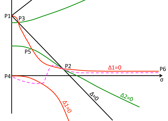
Figure 1. Phase portrait in the range $1<r<r^{*}(d,\ell)$. Dashed curve is the trajectory of the solution constructed in Theorem 2.3.

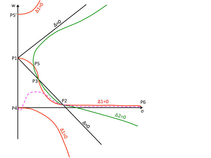
Figure 2. Phase portrait in the range $r^{*}(d,\ell)<r<r_{+}(d,\ell)$, $\ell>d$. Dashed curve is the trajectory of the solution constructed in Theorem 2.3.

2.4. Linearization of the renormalized flow

We aim at building a global in self-similar time $\tau\in[\tau_{0},+\infty)$ solution to (2.7) with non vanishing density $\rho_{T}>0$. We define

$$\left|\begin{array}[]{ll}H_{2}=1+2\frac{\Psi_{P}^{\prime}}{Z}=1-w\\ H_{1}=-\left(\Delta\Psi_{P}+\frac{\ell(r-1)}{2}\right)=H_{2}\frac{\Lambda\rho_{P}}{\rho_{P}}=\frac{\ell}{2}(1-w)\left[1+\frac{\Lambda\sigma}{\sigma}\right]\end{array}\right.$$ (2.25)

We linearize

$$\rho_{T}=\rho_{P}+{\overline{\rho}},\ \ \Psi_{T}=\Psi_{P}+{\overline{\Psi}}.$$ (2.26)

We compute, using the profile equation (2.11), for the first equation:

$$\partial_{\tau}{\overline{\rho}} = -(\rho_{P}+{\overline{\rho}})\Delta(\Psi_{P}+{\overline{\Psi}})-\frac{\ell(r-1)}{2}(\rho_{P}+{\overline{\rho}})-(2\partial_{Z}\Psi_{P}+Z+2\partial_{Z}{\overline{\Psi}})(\partial_{Z}\rho_{P}+\partial_{Z}{\overline{\rho}})$$

$$= -\rho_{T}\Delta{\overline{\Psi}}-2\nabla\rho_{T}\cdot\nabla{\overline{\Psi}}+H_{1}{\overline{\rho}}-H_{2}\Lambda{\overline{\rho}}$$

and for the second one:

$$\partial_{\tau}{\overline{\Psi}} = b^{2}\mathcal{F}(u_{T},\rho_{T})-\Big{\{}|\nabla\Psi_{P}|^{2}+2\nabla\Psi_{P}\cdot\nabla{\overline{\Psi}}+|\nabla{\overline{\Psi}}|^{2}$$

$$+ (r-2)\Psi_{P}+(r-2){\overline{\Psi}}+(\Lambda\Psi_{P}+\Lambda{\overline{\Psi}})+(\rho_{P}+{\overline{\rho}})^{p-1}\Big{\}}$$

$$= b^{2}\mathcal{F}(u_{T},\rho_{T})-\left\{2\nabla\Psi_{P}\cdot\nabla{\overline{\Psi}}+\Lambda{\overline{\Psi}}+(r-2){\overline{\Psi}}+|\nabla{\overline{\Psi}}|^{2}+(\rho_{P}+{\overline{\rho}})^{p-1}-\rho_{P}^{p-1}\right\}$$

$$= b^{2}\mathcal{F}(u_{T},\rho_{T})-\left\{H_{2}\Lambda{\overline{\Psi}}+(r-2){\overline{\Psi}}+|\nabla{\overline{\Psi}}|^{2}+(p-1)\rho_{P}^{p-2}{\overline{\rho}}+\textrm{NL}(\rho)\right\}$$

with

$$\textrm{NL}(\rho)=(\rho_{P}+{\overline{\rho}})^{p-1}-\rho_{P}^{p-1}-(p-1)\rho_{P}^{p-2}{\overline{\rho}}.$$

Hence the exact linearized flow

$$\left|\begin{array}[]{ll}\partial_{\tau}{\overline{\rho}}=H_{1}{\overline{\rho}}-H_{2}\Lambda{\overline{\rho}}-\rho_{T}\Delta{\overline{\Psi}}-2\nabla\rho_{T}\cdot\nabla{\overline{\Psi}}\\ \partial_{\tau}{\overline{\Psi}}=b^{2}\mathcal{F}(u_{T},\rho_{T})-\left\{H_{2}\Lambda{\overline{\Psi}}+(r-2){\overline{\Psi}}+|\nabla{\overline{\Psi}}|^{2}+(p-1)\rho_{P}^{p-2}{\overline{\rho}}+\textrm{NL}(\rho)\right\}\end{array}\right.$$ (2.27)

Theorem 1.1 is therefore equivalent to constructing a finite co-dimensional manifold of smooth well localized initial data leading to global in renormalized $\tau$-time solutions to (2.27).

3. Linear theory slightly beyond the light cone

Our aim in this section is to study the linearized problem (2.27) for the exact Euler problem $b=0$. We in particular aim at setting up the suitable functional framework in order to apply classical propagator estimates which will yield exponential decay on compact sets in $Z$, modulo the control of a finite number of unstable directions. We mainly collect here the results which were proved in detail in [33] and apply verbatim.

3.1. Linearized equations

Recall the exact linearized flow (2.27) which we rewrite:

$$\left|\begin{array}[]{ll}\partial_{\tau}{\overline{\rho}}=H_{1}{\overline{\rho}}-H_{2}\Lambda{\overline{\rho}}-\rho_{P}\Delta{\overline{\Psi}}-2\nabla\rho_{P}\cdot\nabla{\overline{\Psi}}-{\overline{\rho}}\Delta{\overline{\Psi}}-2\nabla{\overline{\rho}}\cdot\nabla{\overline{\Psi}}\\ \partial_{\tau}{\overline{\Psi}}=b^{2}\mathcal{F}(u_{T},\rho_{T})-\left\{H_{2}\Lambda{\overline{\Psi}}+(r-2){\overline{\Psi}}+(p-1)\rho_{P}^{p-2}{\overline{\rho}}+|\nabla{\overline{\Psi}}|^{2}+\textrm{NL}(\rho)\right\}\end{array}\right.$$

We introduce the new unknown

$$\Phi=\rho_{P}{\overline{\Psi}}$$ (3.1)

and obtain equivalently, using (2.25):

$$\left|\begin{array}[]{ll}\partial_{\tau}{\overline{\rho}}=H_{1}{\overline{\rho}}-H_{2}\Lambda{\overline{\rho}}-\Delta\Phi+H_{3}\Phi+G_{\rho}\\ \partial_{\tau}\Phi=-(p-1)Q{\overline{\rho}}-H_{2}\Lambda\Phi+(H_{1}-(r-2))\Phi+G_{\Phi}\end{array}\right.$$ (3.2)

with

$$Q=\rho_{P}^{p-1},\ \ H_{3}=\frac{\Delta\rho_{P}}{\rho_{P}}$$

and the nonlinear terms:

$$\left|\begin{array}[]{ll}G_{\rho}=-{\overline{\rho}}\Delta{\overline{\Psi}}-2\nabla{\overline{\rho}}\cdot\nabla{\overline{\Psi}}\\ G_{\Phi}=-\rho_{P}(|\nabla{\overline{\Psi}}|^{2}+\textrm{NL}(\rho))+b^{2}\rho_{P}\mathcal{F}(u_{T},\rho_{T})\end{array}\right.$$ (3.3)

We transform (3.2) into a wave equation for $\Phi$:

$$\partial_{\tau}^{2}\Phi=(p-1)Q\Delta\Phi-H_{2}^{2}\Lambda^{2}\Phi-2H_{2}\Lambda\partial_{\tau}\Phi+A_{1}\Lambda\Phi+A_{2}\partial_{\tau}\Phi+A_{3}\Phi$$

$$+ \partial_{\tau}G_{\Phi}-\left(H_{1}+H_{2}\frac{\Lambda Q}{Q}\right)G_{\Phi}+H_{2}\Lambda G_{\Phi}-(p-1)QG_{\rho}$$

with

$$\left|\begin{array}[]{llll}A_{1}=H_{2}H_{1}-H_{2}\Lambda H_{2}+H_{2}(H_{1}-(r-2))+H_{2}^{2}\frac{\Lambda Q}{Q}\\ A_{2}=2H_{1}-(r-2)+H_{2}\frac{\Lambda Q}{Q}\\ A_{3}=-(H_{1}-(r-2))H_{1}+H_{2}\Lambda H_{1}-H_{2}(H_{1}-(r-2))\frac{\Lambda Q}{Q}-(p-1)QH_{3}\end{array}\right.$$

Remark 3.1 (Null coordinates and red shift).

We note that the principal symbol of the above wave equation is given by the second order operator

$$\Box_{Q}:=\partial_{\tau}^{2}-((p-1)Q-H_{2}^{2}Z^{2})\partial_{Z}^{2}+2H_{2}Z\partial_{Z}\partial_{\tau}.$$

This operator governs propagation of sound waves associated to the background solution $(\rho_{P},\Psi_{P})$ of the Euler equations.

In the variables of Emden transform $(\tau,y={\rm log}Z)$, $\Box_{Q}$ can be written equivalently as

$$\Box_{Q}=\partial_{\tau}^{2}-\left[\sigma^{2}-(1-w)^{2}\right]\partial_{y}^{2}+2(1-w)\partial_{y}\partial_{\tau}$$

The two principal null direction associated with the above equation are

$$L=\partial_{\tau}+\left[(1-w)-\sigma\right]\partial_{y},\qquad\underline{L}=\partial_{\tau}+\left[(1-w)+\sigma\right]\partial_{y},$$

so that

$$\Box_{Q}=L\underline{L}$$

We observe that at $P_{2}$, we have $L=\partial_{\tau}$ and the surface $Z=Z_{2}$ is a null cone. Moreover, the associated acoustical metric is

$$g_{Q}=\Delta d\tau^{2}-2(1-w)d\tau dy+dy^{2},\qquad\Delta=(1-w)^{2}-\sigma^{2}$$

for which $\partial_{\tau}$ is a Killing field (generator of translation symmetry). Therefore, $Z=Z_{2}$ is a Killing horizon (generated by a null Killing field.) We can make it even more precise by transforming the metric $g_{Q}$ into a slightly different form by defining the coordinate $s$:

$$s=\tau-f(y),\qquad f^{\prime}=\frac{1-w}{\Delta},$$

so that

$$g_{Q}=\Delta(ds)^{2}-\frac{\sigma^{2}}{\Delta}dy^{2}$$

and then the coordinate $y^{*}$:

$$y^{*}=\int\frac{\sigma}{\Delta}dy,$$

so that

$$g_{Q}=\Delta\,d(s+y^{*})\,d(s-y^{*})$$

and $y+x^{*}$ and $y-x^{*}$ are the null coordinates of $g_{Q}$. The Killing horizon $Z=Z_{2}$ corresponds to $y^{*}=-\infty$ and $\Delta\sim e^{Cy^{*}}$ for some positive constant $C$. In this form, near $Z_{2}$ the metric $g_{Q}$ resembles the $1+1$-quotient Schwarzschild metric near the black hole horizon.

The associated surface gravity $\kappa$ which can be computed according to

$$\kappa =\frac{\partial_{y^{*}}\Delta}{2\Delta}|_{P_{2}}=\frac{\partial_{y}\Delta}{2\sigma}|_{P_{2}}=\frac{-w^{\prime}(1-w)-\sigma^{\prime}\sigma)}{\sigma}|_{P_{2}}$$

$$=(-w^{\prime}-\sigma^{\prime})|_{P_{2}}=1-w-\Lambda w-\frac{(1-w)F}{\sigma}|_{P_{2}}>0$$

This is precisely the repulsive condition (2.23) (at $P_{2}$). The positivity of surface gravity implies the presence of the red shift effect along $Z=Z_{2}$ both as an optical phenomenon for the acoustical metric $g_{Q}$ and also as an indicator of local monotonicity estimates for solutions of the wave equation $\Box_{Q}\varphi=0$, [17]. The complication in the analysis below is the presence of lower order terms in the wave equation as well as the need for global in space estimates.

We focus now on deriving decay estimates for (3.2).

3.2. The linearized operator with a shifted measure

Pick a small enough parameter

$$0<a\ll 1$$

and consider the new variable

$$\Theta=\partial_{\tau}\Phi+aH_{2}\Lambda\Phi,$$ (3.4)

we compute the $(\Theta,\Phi)$ equation

$$\partial_{\tau}X=\mathcal{M}X+G,\ \ X=\left|\begin{array}[]{ll}\Phi\\ \Theta\end{array}\right.,\ \ G=\left|\begin{array}[]{ll}0\\ G_{\Theta}\end{array}\right.$$ (3.5)

with

$$\mathcal{M}=\left(\begin{array}[]{ll}-aH_{2}\Lambda&1\\ (p-1)Q\Delta-(1-a)^{2}H_{2}^{2}\Lambda^{2}+\tilde{A_{2}}\Lambda+A_{3}&-(2-a)H_{2}\Lambda+A_{2}\end{array}\right)$$ (3.6)

where

$$G_{\Theta}=\partial_{\tau}G_{\Phi}-\left(H_{1}+H_{2}\frac{\Lambda Q}{Q}\right)G_{\Phi}+H_{2}\Lambda G_{\Phi}-(p-1)QG_{\rho}$$ (3.7)

and

$$\tilde{A}_{2}=A_{1}+(2a-a^{2})H_{2}\Lambda H_{2}-aA_{2}H_{2}.$$

The fine structure of the operator (3.6) involves the understanding of the associated shifted light cone.

Lemma 3.2 (Shifted measure, [33]).

Let

$$D_{a}=(1-a)^{2}(w-1)^{2}-\sigma^{2}$$ (3.8)

then for $0<a<a^{*}$ small enough, there exists a $\mathcal{C}^{1}$ map $a\mapsto Z_{a}$ with

$$Z_{a=0}=Z_{2},\ \ \frac{\partial Z_{a}}{\partial a}>0$$

such that

$$\left|\begin{array}[]{l}D_{a}(Z_{a})=0\\ -D_{a}(Z)>0\ \ \mbox{on}\ \ 0\leq Z<Z_{a}\\ \mathop{\rm lim}_{Z\to 0}Z^{2}(-D_{a})>0.\end{array}\right.$$ (3.9)

3.3. Commuting with derivatives

We define

$$\Theta_{k}=\Delta^{k}\Theta,\ \ \Phi_{k}=\Delta^{k}\Phi$$

and commute the linearized flow with derivatives.

Lemma 3.3 (Commuting with derivatives, [33]).

Let $k\in\mathbb{N}$. There exists a smooth measure $g$ defined for $Z\in[0,Z_{a}]$ such that the following holds. Let

$$\mathcal{L}_{g}\Phi_{k}=\frac{1}{gZ^{d-1}}\partial_{Z}\left(Z^{d-1}Z^{2}g(-D_{a})\partial_{Z}\Phi_{k}\right),$$

then there holds

$$\Delta^{k}(\mathcal{M}X)=\mathcal{M}_{k}\left|\begin{array}[]{ll}\Phi_{k}\\ \Theta_{k}\end{array}\right.+\widetilde{\mathcal{M}}_{k}X$$ (3.10)

with

$$\mathcal{M}_{k}\left|\begin{array}[]{ll}\Phi_{k}\\ \Theta_{k}\end{array}\right.=\left|\begin{array}[]{ll}-aH_{2}\Lambda\Phi_{k}-2ak(H_{2}+\Lambda H_{2})\Phi_{k}+\Theta_{k}\\ \mathcal{L}_{g}\Phi_{k}-(2-a)H_{2}\Lambda\Theta_{k}-2k(2-a)(H_{2}+\Lambda H_{2})\Theta_{k}+A_{2}\Theta_{k}\end{array}\right.$$

where $\widetilde{\mathcal{M}}_{k}$ satisfies the following pointwise bound

$$|\widetilde{\mathcal{M}}_{k}X|\lesssim_{k}\left|\begin{array}[]{ll}\displaystyle\sum_{j=0}^{2k-1}|\partial^{j}_{Z}\Phi|,\\ \displaystyle\sum_{j=0}^{2k}|\partial^{j}_{Z}\Phi|+\sum_{j=0}^{2k-1}|\partial_{Z}^{j}\Theta|.\end{array}\right.$$ (3.11)

Moreover, $g>0$ in $[0,Z_{a})$ and admits the asymptotics:

$$\left|\begin{array}[]{ll}g(Z)=1+O(Z^{2})\ \ \mbox{as}\ \ Z\to 0\\ g(Z)=c_{a,d,r,\ell}(Z_{a}-Z)^{c_{g}}\left[1+O(Z-Z_{a})\right]\ \mbox{as}\ \ Z\uparrow Z_{a},\ \ .\end{array}\right.$$ (3.12)

with

$$c_{g}>0$$ (3.13)

for all $k\geq k_{1}$ large enough and $0<a<a^{*}$ small enough.

3.4. Maximal accretivity and spectral gap

The linear theory we use relies on the spectral structure of compact perturbations of maximal accretive operators.

Hilbert space. We define the space of test functions

$$\mathcal{D}_{0}=\mathcal{D}_{\Phi}\times C_{\rm radial}^{\infty}([0,Z_{a}],\mathbb{C}),$$

and let ${\mathbb{H}}_{2k}$ be the completion of $\mathcal{D}_{0}$ for the scalar product:

$$\langle X,\tilde{X}\rangle=\langle\langle\Phi,\Phi\rangle\rangle+(\Theta_{k},\tilde{\Theta}_{k})_{g}+\int\chi\Theta\overline{\tilde{\Theta}}Z^{d-1}dZ$$ (3.14)

where

$$\langle\langle\Phi,\tilde{\Phi}\rangle\rangle = -(\mathcal{L}_{g}\Phi_{k},\tilde{\Phi}_{k})_{g}+\int\chi\Phi\overline{\tilde{\Phi}}gZ^{d-1}dZ,$$ (3.15)

$$(\Theta_{k},\tilde{\Theta}_{k})_{g}=\int\Theta_{k}\overline{\tilde{\Theta}_{k}}gZ^{d-1}dZ,$$

$\chi$ be a smooth cut off function supported on the set $|Z|<Z_{2}$ such that

$$g\geq\frac{1}{2}\ \ \mbox{on}\ \ {\rm Supp}\chi.$$

Unbounded operator. Following (3.6) we define the operator

$$\ \ \mathcal{M}=\left(\begin{array}[]{ll}-aH_{2}\Lambda&1\\ (p-1)Q\Delta-(1-a)^{2}H_{2}^{2}\Lambda^{2}+\tilde{A_{2}}\Lambda+A_{3}&-(2-a)H_{2}\Lambda{+A_{2}}\end{array}\right)$$

with domain

$$D(\mathcal{M})=\{X\in\mathbb{H}_{2k},\ \ \mathcal{M}X\in\mathbb{H}_{2k}\}$$ (3.16)

equipped with the domain norm. We then pick suitable directions $(X_{i})_{1\leq i\leq N}\in\mathbb{H}_{2k}$ and consider the finite rank projection operator

$$\mathcal{A}=\sum_{i=1}^{N}\langle\cdot,X_{i}\rangle X_{i}.$$

The following fundamental accretivity property is proved in [33].

Proposition 3.4 (Maximal accretivity/dissipativity, [33]).

There exist $k_{\flat}\gg 1$ and $0<c^{*},a^{*}\ll 1$ such that for all $k\geq k_{\flat}$, $\forall 0<a<a^{*}$ small enough, there exist $N=N(k,a)$ directions $(X_{i})_{1\leq i\leq N}\in\mathbb{H}_{2k}$ such that the modified unbounded operator

$$\tilde{\mathcal{M}}:={\mathcal{M}-}\mathcal{A}$$

is dissipative

$$\forall X\in\mathcal{D}(\mathcal{M}),\ \ \Re\langle(-\mathcal{\tilde{M}}X,X\rangle\geq c^{*}ak\langle X,X\rangle$$ (3.17)

and maximal:

$$\forall R>0,\ \ \forall F\in\mathbb{H}_{2k},\ \ \exists X\in\mathcal{D}(\mathcal{M})\ \ \mbox{such that}\ \ (-\tilde{\mathcal{M}}+R)X=F.$$ (3.18)

Exponential decay in time locally in space will now follow from the following classical statement, see [18, 33] for a detailed proof.

Lemma 3.5 (Exponential decay modulo finitely many instabilities).

Let $\delta_{g}>0$ and let $T_{0}$ be the strongly continuous semigroup generated by a maximal dissipative operator $\tilde{\mathcal{M}}+\delta_{g}$, and $T$ be the strongly continuous semi group generated by ${\mathcal{M}}=\tilde{\mathcal{M}}+A$ where $A$ is a compact operator on $H$. Then the following holds:
(i) the set $\Lambda_{\delta_{g}}(\mathcal{M})=\sigma(A)\cap\{\lambda\in\mathbb{C},\ \ \Re(\lambda)>-\frac{\delta_{g}}{2}\}$ is finite, each eigenvalue $\lambda\in\Lambda_{\delta_{g}}(\mathcal{M})$ has finite algebraic multiplicity $k_{\lambda}$. In particular, the subspace $V_{\delta_{g}}(\mathcal{M})$ is finite dimensional;
(ii) We have $\Lambda_{\delta_{g}}(\mathcal{M})=\overline{\Lambda_{\delta_{g}}(\mathcal{M}^{*})}$ and $dimV_{\delta_{g}}(\mathcal{M}^{*})=dimV_{\delta_{g}}(\mathcal{M})$. The direct sum decomposition

$$H=V_{\delta_{g}}(\mathcal{M})\bigoplus V^{\perp}_{\delta_{g}}(\mathcal{M}^{*})$$ (3.19)

is preserved by $T(t)$ and there holds:

$$\forall X\in V^{\perp}_{\delta_{g}}(\mathcal{M}^{*}),\ \ \|T(t)X\|\leq M_{\delta_{g}}e^{-\frac{\delta_{g}}{2}t}\|X\|.$$ (3.20)

(iii) The restriction of $A$ to $V_{\delta_{g}}(\mathcal{M})$ is given by a direct sum of $(m_{\lambda}\times m_{\lambda})_{\lambda\in\Lambda_{\delta_{g}}(\mathcal{M})}$ matrices each of which is the Jordan block associated to the eigenvalue $\lambda$ and the number of Jordan blocks corresponding to $\lambda$ is equal to the geometric multiplicity of $\lambda$ – $m^{g}_{\lambda}=dimker(\mathcal{M}-\lambda I)$. In particular, $m^{a}_{\lambda}\leq m^{g}_{\lambda}k_{\lambda}$. Each block corresponds to an invariant subspace $J_{\lambda}$ and the semigroup $T$ restricted to $J_{\lambda}$ is given by the nilpotent matrix

$$T(t)|_{J_{\lambda}}=\begin{pmatrix}e^{\lambda t}&te^{\lambda t}&...&t^{m_{\lambda}-1}e^{\lambda t}\\ 0&e^{\lambda t}&...&t^{m_{\lambda}-2}e^{\lambda t}\\ ...\\ 0&0&...&e^{\lambda t}\end{pmatrix}$$

Our final result in this section is a Brouwer type argument for the evolution of unstable modes.

Lemma 3.6 (Brouwer argument, [33]).

Let $A,\delta_{g}$ as in Lemma 3.5 with the decomposition

$$H=U\bigoplus V$$

into stable and unstable subspaces Fix sufficiently large $t_{0}>0$ (dependent on $A$). Let $F(t)$ such that, $\forall t\geq t_{0}$, $F(t)\in V$ and

$$\|F(t)\|\leq e^{-\frac{2\delta_{g}}{3}t}$$

be given. Let $X(t)$ denote the solution to the ode

$$\left|\begin{array}[]{l}\frac{dX}{dt}=AX+F(t)\\ X(t_{0})=x\in V.\end{array}\right.$$

Then, for any $x$ in the ball

$$\|x\|\leq e^{-\frac{3\delta_{g}}{5}t_{0}},$$

we have

$$\|X(t)\|\leq e^{-\frac{\delta_{g}}{2}t},\qquad t_{0}\leq t\leq t_{0}+\Gamma$$ (3.21)

for some large constant $\Gamma$ (which only depends on $A$ and $t_{0}$.) Moreover, there exists $x^{*}\in V$ in the same ball as a above such that $\forall t\geq t_{0}$,

$$\|X(t)\|\leq e^{-\frac{3\delta_{g}}{5}t}$$

4. Setting up the bootstrap

In this section we detail the set of smooth well localized initial data which lead to the conclusions of Theorem 1.1.

4.1. Cauchy theory and renormalization

We use local Cauchy theory for strong solutions for Navier-Stokes from [15].

Theorem 4.1 (Local Cauchy theory NS, [15]).

Assume

$$\left|\begin{array}[]{l}\rho_{0}\in H^{1}\cap W^{1,6}\\ u_{0}\in\dot{H^{1}}\cap\dot{H}^{2}\\ \frac{-\Delta u_{0}+\nabla p_{0}}{\sqrt{\rho_{0}}}\in L^{2}\end{array}\right.$$ (4.1)

then there exists a unique local strong solution $(\rho,u)\in L^{\infty}([0,T)\cap H^{1}\cap W^{1,6})\times L^{\infty}([0,T),\dot{H^{1}}\cap\dot{H}^{2})$ to (1.1). Moreover, the maximal time of existence $T$ is characterized by the condition

$$\int_{0}^{T}\|\nabla u\|_{L^{\infty}(\mathbb{R}^{3})}=\infty$$ (4.2)

In the Euler case we can use the results from [27] and [8]

Theorem 4.2 (Local Cauchy theory, Euler, [27, 8]).

Assume

$$\rho^{\frac{\gamma-1}{2}}_{0},u_{0}\in H^{s}$$ (4.3)

for some $s>1+\frac{d}{2}$, then there exists a unique local strong solution $(\rho^{\frac{\gamma-1}{2}},u)\in C^{0}([0,T)\cap H^{s})$ to (1.2). Moreover, the maximal time of existence $T$ is characterized by the condition

$$\int_{0}^{T}\|\nabla u\|_{L^{\infty}(\mathbb{R}^{d})}=\infty$$ (4.4)

On an interval $[0,T^{*}]$, $T^{*}\leq T$, where $\rho(t,x)$ does not vanish, we equivalently work with (2.4) and proceed to the decomposition of Lemma 2.1

$$\left|\begin{array}[]{l}\hat{\rho}(t,x)=\left(\frac{\lambda}{\nu}\right)^{\frac{1}{\gamma-1}}\rho_{T}(\tau,Z)\\ \hat{u}(t,x)=\frac{\lambda}{\nu}u_{T}(s,Z),\ \ u_{T}=\nabla\Psi_{T}=U_{T}\vec{e}_{r}\end{array}\right.$$

with the renormalization:

$$\left|\begin{array}[]{lll}Z=y\sqrt{b}=Z^{*}x,\ \ Z^{*}=\frac{1}{\lambda}=e^{\tau}\\ \lambda(\tau)=e^{-\tau},\ \ \nu(\tau)=e^{-r\tau},\ \ b(\tau)=e^{-e\tau}\\ \tau=\frac{-{\rm log}(T-t)}{r},\ \ \tau_{0}=\frac{-{\rm log}T}{r}.\end{array}\right.$$ (4.5)

Our claim is that given

$$\tau_{0}=\frac{-{\rm log}T}{r}$$

large enough, we can construct a finite co-dimensional manifold of smooth well localized initial data $(\hat{\rho}_{0},\hat{u}_{0})$ such that the corresponding solution to the renormalized flow (2.7) is global $\tau\in[\tau_{0},+\infty)$, bounded in a suitable topology and non vanishing. Going back to the original variables yields a solution to (1.1) which blows up at $T$ in the regime described by Theorem 1.1.

4.2. Regularity and dampening of the profile outside the singularity

The profile solution $(\rho_{P},\Psi_{P})$ has an intrinsic slow decay as $Z\to+\infty$ forced by the self similar equation

$$\rho_{P}(Z)=\frac{c_{P}}{\langle Z\rangle^{\frac{2(r-1)}{p-1}}}\left(1+O\left(\frac{1}{\langle Z\rangle^{r}}\right)\right)$$

which need be regularized in order to produce finite energy non vanishing initial data.

1. Regularity of the profile. Recall the asymptotics (2.21) and the choice of parameters (2.5) which show that in the original variables $(t,x)$ both the density and the velocity profiles are regular away from the singular point $x=0$:

$$\rho_{P}(t,x)=\left(\frac{\lambda}{\nu}\right)^{\frac{1}{\gamma-1}}\rho_{P}\left(\frac{x}{\lambda}\right)=\frac{c_{\rho}e^{\frac{(r-1)}{\gamma-1}\tau}}{Z^{\frac{2(r-1)}{p-1}}}\left[1+O\left(\frac{1}{\langle Z\rangle^{r}}\right)\right]$$ (4.6)

$$= \frac{c_{\rho}}{|x|^{\frac{2(r-1)}{p-1}}}\left[1+O\left(\frac{1}{\langle Z\rangle^{r}}\right)\right]$$

and

$$U_{P}(t,x) = \frac{\lambda}{\nu}\partial_{Z}\Psi_{P}\left(\frac{x}{\lambda}\right)=e^{(r-1)\tau}\frac{c_{\Psi}}{Z^{r-1}}\left[1+O\left(\frac{1}{\langle Z\rangle^{r}}\right)\right]$$ (4.7)

$$= \frac{c_{\Psi}}{x^{r-1}}\left[1+O\left(\frac{1}{\langle Z\rangle^{r}}\right)\right]$$

2. Dampening of the tail. The above regularity allows us to turn our profile into a finite energy (and better) solution. We dampen the tail outside the singularity $x\geq 1$, i.e., $Z\geq Z^{*}$ as follows. Let

$$\mathcal{K}_{\rho}(x)=\left|\begin{array}[]{ll}0\ \ \mbox{for}\ \ |x|\leq 5\\ n_{P}-\frac{2(r-1)}{p-1}\ \ \mbox{for}\ \ |x|\geq 10\end{array}\right.,$$ (4.8)

for some large enough universal constant

$$n_{P}=n_{P}(d)\gg 1.$$

We then define the dampened tail profile $\rho_{D}$: in the original variables

$$\hat{\rho}_{D}(t,x)=\hat{\rho}_{P}(t,x)e^{-\int_{0}^{x}\frac{\mathcal{K}_{\rho}(x^{\prime})}{x^{\prime}}dx^{\prime}}=\left|\begin{array}[]{ll}\hat{\rho}_{P}(t,x)\ \ \mbox{for}\ \ |x|\leq 5\\ \frac{c_{n,\delta}}{|x|^{n_{P}}}\left[1+O\left(e^{-r\tau})\right)\right]\ \ \mbox{for}\ \ |x|\geq 10\end{array}\right.,$$ (4.9)

and in the renormalized variables:

$$\rho_{D}(\tau,Z)=\left(\frac{\nu}{\lambda}\right)^{\frac{2}{p-1}}\hat{\rho}_{D}(t,x),\ \ x=\frac{Z}{Z^{*}}.$$ (4.10)

Let

$$\zeta(x)=e^{-\int_{0}^{x}\frac{\mathcal{K}_{\rho}(x^{\prime})}{x^{\prime}}dx^{\prime}},$$

we have the equivalent representation:

$$\rho_{D}(\tau,Z)=(\lambda\sqrt{b})^{\frac{2}{p-1}}\hat{\rho}_{D}(\tau,x)=(\lambda\sqrt{b})^{\frac{2}{p-1}}\hat{\rho}_{P}(t,x)\zeta(x)=\zeta(\lambda Z)\rho_{P}(Z)$$ (4.11)

Note that by construction for $j\in\mathbb{N}^{*}$:

$$-\frac{Z^{j}\partial^{j}_{Z}\rho_{D}}{\rho_{D}}=\left|\begin{array}[]{ll}\ \ (-1)^{j-1}\left(\frac{2(r-1)}{p-1}\right)^{j}+O\left(\frac{1}{\langle Z\rangle^{r}}\right)\ \ \mbox{for}\ \ Z\leq 5Z^{*}\\ (-1)^{j-1}n_{P}^{j}+O\left(\frac{1}{\langle Z\rangle^{r}}\right)\mbox{for}\ \ Z\geq 10Z^{*}\end{array}\right.$$ (4.12)

and

$$\left|\frac{\langle Z\rangle^{j}\partial_{j}\rho_{D}}{\rho_{D}}\right|_{L^{\infty}}\lesssim c_{j}.$$ (4.13)

We proceed similarly for the velocity profile which can be even made compactly supported. Let

$$\zeta_{u}(x)=\left|\begin{array}[]{ll}1\ \ \mbox{for}\ \ |x|\leq 5\\ 0\ \ \mbox{for}\ \ |x|\geq 10\end{array}\right.,$$

and define

$$U_{D}(t,x)=\hat{U}_{P}(t,x)\zeta_{u}(x)=\left|\begin{array}[]{ll}\hat{U}_{P}(t,x)\ \ \mbox{for}\ \ |x|\leq 5\\ 0\ \ \mbox{for}\ \ |x|\geq 10\end{array}\right.,$$ (4.14)

and thus in renormalized variables:

$$U_{D}(\tau,Z)=\frac{\nu}{\lambda}\hat{U}_{D}(t,x)=\zeta_{u}(\lambda Z)U_{P}(Z),\ \ x=\frac{Z}{Z^{*}}.$$ (4.15)

We then let

$$\Psi_{D}(\tau,Z)=-\frac{1}{r-2}+\int_{0}^{Z}U_{D}(\tau,z)dz$$

so that by construction $\Psi_{D}=\Psi_{P}$ for $Z\leq 5Z^{*}$.

4.3. Initial data

We now describe explicitly open set of initial data which are perturbations of the profile $(\rho_{D},\Psi_{D})$ in a suitable topology. The conclusions of Theorem 1.1 will hold for a finite co-dimension set of such data. Our first restriction is that the initial data $(\rho_{0},u_{0})$ in the original, non-renormalized variables satisfy the assumptions (4.1) and (4.3) for the validity of the local Cauchy theory.

We now pick universal constants $0<a\ll 1$, $Z_{0}\gg 1$ which will be adjusted along the proof and depend only on $(d,\ell)$. We define two levels of regularity

$$\frac{d}{2}\ll k_{\flat}\ll{k^{\sharp}}$$

where ${k^{\sharp}}$ denotes the maximum level of regularity required for the solution and $k_{\flat}$ is the level of regularity required for linear spectral theory on a compact set.

0. Variables and notations for derivatives. We define the variables

$$\left|\begin{array}[]{l}\rho_{T}=\rho_{D}+\tilde{\rho}\\ \Psi_{T}=\Psi_{D}+\tilde{\Psi}\\ u_{D}=\nabla\Psi_{D},\ \ \tilde{u}=\nabla\tilde{\Psi}\\ U_{D}=\partial_{Z}\Psi_{D},\ \ \tilde{U}=\partial_{Z}\tilde{\Psi}\\ \Phi=\rho_{P}\Psi\end{array}\right.$$ (4.16)

and specify the data in the $(\tilde{\rho},\tilde{\Psi})$ variables. We will use the following notations for derivatives. Given $k\in\mathbb{N}$, we note

$$\partial^{k}=(\partial_{1}^{k},...,\partial_{d}^{k}),\ \ f^{(k)}:=\partial^{k}f$$

the vector of $k$-th derivatives in each direction. The notation $\partial_{Z}^{k}f$ is the $k$-th radial derivative. We let

$$\tilde{\rho}_{k}=\Delta^{k}\tilde{\rho},\qquad\tilde{\Psi}_{k}=\Delta^{k}\Psi.$$

Given a multiindex $\alpha=(\alpha_{1},\ldots,\alpha_{d})\in\mathbb{N}^{d}$, we note

$$\nabla^{\alpha}=\partial^{\alpha_{1}}_{1}\dots\partial^{\alpha_{d}}_{d},\ \ |\alpha|=\alpha_{1}+\dots+\alpha_{d}.$$

Sometimes, we will use the notation $\nabla^{k}$ to denote a $\nabla^{\alpha}$ derivatives of order $k=|\alpha|$.

1. Initializing the Brouwer argument. We define the variables adapted to the spectral analysis according to (3.1), (3.4):

$$\left|\begin{array}[]{ll}\Phi=\rho_{P}\Psi\\ T=\partial_{\tau}\Phi+aH_{2}\Lambda\Phi\end{array}\right.,\ \ X=\left|\begin{array}[]{ll}\Phi\\ \Theta\end{array}\right.$$ (4.17)

and recall the scalar product (3.14). For $0<c_{g},a\ll 1$ small enough, we choose $k_{\flat}\gg 1$ such that Proposition 3.4 applies in the Hilbert space $\mathbb{H}_{2k_{\flat}}$ with the spectral gap

$$\forall X\in\mathcal{D}(\mathcal{M}),\ \ \Re\langle(-\mathcal{M}+\mathcal{A})X,X\rangle\geq c_{g}\langle X,X\rangle.$$ (4.18)

Hence

$$\mathcal{M}=(\mathcal{M}-\mathcal{A}+c_{g})-c_{g}+\mathcal{A}$$

and we may apply Lemma 3.5:

$$\Lambda_{0}=\{\lambda\in\mathbb{C},\ \ \Re(\lambda)\geq 0\}\cap\{\lambda\ \ \mbox{is an eigenvalue of}\ \ \mathcal{M}\}=(\lambda_{i})_{1\leq i\leq N}$$ (4.19)

is a finite set corresponding to unstable eigenvalues, $V$ is an associated (unstable) finite dimensional invariant set, $U$ is the complementary (stable) invariant set

$$\mathbb{H}_{2k_{\flat}}=U\bigoplus V$$ (4.20)

and $P$ is the associated projection on $V$. We denote by ${\mathcal{N}}$ the nilpotent part of the matrix representing ${\mathcal{M}}$ on V:

$${\mathcal{M}}|_{V}={\mathcal{N}}+{\text{diag}}$$ (4.21)

Then there exist $C,\delta_{g}>0$ such that (3.20) holds:

$$\forall X\in U,\ \ \|e^{\tau\mathcal{M}}X\|_{\mathbb{H}_{2k_{\flat}}}\leq Ce^{-\frac{\delta_{g}}{2}\tau}\|X\|_{\mathbb{H}_{2k_{\flat}}},\qquad\forall\tau\geq\tau_{0}.$$

We now choose the data at $\tau_{0}$ such that

$$\|(I-P)X(\tau_{0})\|_{\mathbb{H}_{2k_{\flat}}}\leq e^{-\frac{\delta_{g}}{2}\tau_{0}},\qquad\|PX(\tau_{0})\|_{\mathbb{H}_{2k_{\flat}}}\leq e^{-\frac{3\delta_{g}}{5}\tau_{0}}.$$

2. Bounds on local low Sobolev norms. Let $0\leq m\leq 2k_{\flat}$ and

$$\nu_{0}=-\frac{2(r-1)}{p-1}+\frac{\delta_{g}}{2},$$ (4.22)

let the weight function

$$\xi_{\nu_{0},m}=\frac{1}{\langle Z\rangle^{d-2(r-1)+2(\nu_{0}-m)}}\zeta\left(\frac{Z}{Z^{*}}\right),\ \ \zeta(Z)=\left|\begin{array}[]{ll}1\ \ \mbox{for}\ \ Z\leq 2\\ 0\ \ \mbox{for}\ \ Z\geq 3.\end{array}\right.$$ (4.23)

Then:

$$\sum_{m=0}^{2k_{\flat}}\int\xi_{\nu_{0},m}\left((p-1)\rho_{P}^{p-1}(\nabla^{m}\rho(\tau_{0}))^{2}+|\nabla\nabla^{m}\Phi(\tau_{0})|^{2}\right)\leq e^{-\delta_{g}\tau_{0}}.$$ (4.24)

3. Pointwise assumptions. We assume the following interior pointwise bounds

$$\forall 0\leq k\leq 2k^{\sharp},\ \ \left\|\frac{\langle Z\rangle^{k}\partial_{Z}^{k}\tilde{\rho}(\tau_{0})}{\rho_{D}}\right\|_{L^{\infty}(Z\leq Z^{*}_{0})}+\left\|{\langle Z\rangle^{r-1}}\langle Z\rangle^{k}\nabla^{k}\tilde{u}(\tau_{0})\right\|_{L^{\infty}(Z\leq Z^{*}_{0})}\leq\lambda_{0}^{c_{0}}$$ (4.25)

for some small enough universal constant $c_{0}$, and the exterior bounds:

$$\forall 0\leq k\leq 2{k^{\sharp}},\ \ \left\|\frac{Z^{k+1}\partial_{Z}^{k}\tilde{\rho}(\tau_{0})}{\rho_{D}}\right\|_{L^{\infty}(Z\geq Z^{*}_{0})}+\frac{\|Z^{k{+1}}\nabla^{k}\tilde{u}(\tau_{0})\|_{L^{\infty}(Z\geq Z^{*}_{0})}}{\lambda_{0}^{r-1}}\leq\lambda_{0}^{C_{0}}$$ (4.26)

for some large enough universal $C_{0}(d,r,\ell)$. Note in particular that (4.25), (4.26) ensure that for all $0<\lambda_{0}$ small enough:

$$\left\|\frac{\tilde{\rho}(\tau_{0})}{\rho_{D}}\right\|_{L^{\infty}}\leq\mathcal{d}_{0}\ll 1$$ (4.27)

and hence the data does not vanish.

4. Global bounds for high energy norms. We pick a large enough constant ${k^{\sharp}}(d,r,\ell)$ and consider the global energy norm

$$\|\tilde{\rho},\tilde{\Psi}\|_{{k^{\sharp}}}^{2}:=\sum_{j=0}^{{k^{\sharp}}}\sum_{|\alpha|=j}\int\frac{(p-1)\rho_{D}^{p-2}\rho_{T}(\nabla^{\alpha}\tilde{\rho})^{2}+\rho_{T}^{2}|\nabla\nabla^{\alpha}\Psi|^{2}}{\langle Z\rangle^{2({k^{\sharp}}-j)}},$$ (4.28)

then we require:

$$\|\tilde{\rho}(\tau_{0}),\tilde{\Psi}(\tau_{0})\|_{{k^{\sharp}}}\leq\mathcal{d}_{0}$$ (4.29)

We now define the weight functions

$$\chi_{k}=\langle Z\rangle^{2k-2\sigma-d+\frac{2(r-1)(p+1)}{p-1}}\left\langle\frac{Z}{Z^{*}}\right\rangle^{2n_{P}+2\sigma-\frac{2(r-1)(p+1)}{p-1}}$$ (4.30)

and the associated weighted energy norms

$$\|\tilde{\rho},\tilde{\Psi}\|_{m,\sigma}^{2}=\sum_{j=0}^{m}\sum_{|\alpha|=j}\int\chi_{j}\left[(p-1)\rho_{D}^{p-2}\rho_{T}|\nabla^{\alpha}\tilde{\rho}|^{2}+\rho_{T}^{2}|\nabla\nabla^{\alpha}\tilde{\Psi}|^{2}\right]$$ (4.31)

We fix $0<\sigma({k^{\sharp}})\ll\delta_{g}$ and require that, for $\sigma=\sigma({k^{\sharp}})$,

$$\|\tilde{\rho}(\tau_{0}),\tilde{\Psi}(\tau_{0})\|_{{k^{\sharp}},\sigma}\leq\mathcal{d}_{0}e^{-\sigma\tau_{0}}$$ (4.32)

Remark 4.3.

$\mathcal{d}_{0}$ will denote any small constant dependent on the smallness of initial data and $\tau_{0}^{-1}$.

Remark 4.4.

We note that a straightforward integration by parts and induction argument implies that the norms $\|\tilde{\rho},\tilde{\Psi}\|_{m,\sigma}$ and $\|\tilde{\rho},\tilde{\Psi}\|_{{k^{\sharp}}}$ are equivalent to the ones with $\nabla^{\alpha}\tilde{\rho}$ and $\nabla^{\alpha}\tilde{\Psi}$ replaced by

$$\partial^{j}\tilde{\rho}=\{\partial_{1}^{j},...,\partial_{d}^{j}\tilde{\rho}\},\qquad\partial^{j}\tilde{\Psi}=\{\partial_{1}^{j},...,\partial_{d}^{j}\tilde{\Psi}\}$$

as well as $\Delta^{j}\tilde{\rho},\Delta^{j}\tilde{\Psi}$ with $j$ varying from $0$ to $\frac{m}{2}$ and $\frac{{k^{\sharp}}}{2}$ respectively (if $m$ and ${k^{\sharp}}$ are even.) In what follows, we will use this equivalence continually and without mentioning. In fact, in what follows we will specifically work with the norms

$$\|\tilde{\rho},\tilde{\Psi}\|_{{k^{\sharp}}}^{2}:=\sum_{j=0}^{\frac{{k^{\sharp}}}{2}}\int\frac{(p-1)\rho_{D}^{p-2}\rho_{T}(\Delta^{j}\tilde{\rho})^{2}+\rho_{T}^{2}|\nabla\Delta^{j}\Psi|^{2}}{\langle Z\rangle^{2({k^{\sharp}}-2j)}}$$

and

$$\|\tilde{\rho},\tilde{\Psi}\|_{m,\sigma}^{2}=\sum_{j=0}^{m}\int\chi_{j}\left[(p-1)\rho_{D}^{p-2}\rho_{T}|\partial^{j}\tilde{\rho}|^{2}+\rho_{T}^{2}|\nabla\partial^{j}\tilde{\Psi}|^{2}\right]$$

4.4. Bootstrap bounds

Since the initial data satisfy (4.1) we have a local in time solution which can be decomposed and renormalized according to (4.5) and (4.16). We now consider the time interval $[\tau_{0},\tau^{*})$ such that the following bounds hold on $[\tau_{0},\tau^{*})$:

1. Control of the unstable modes: Assume (see (4.21)) that

$$\|e^{t{\mathcal{N}}}PX(\tau)\|_{\mathbb{H}_{2k_{\flat}}}\leq e^{-\frac{19\delta_{g}}{30}\tau}$$ (4.33)

2. Local decay of low Sobolev norms: for any $0\leq k\leq 2k_{\flat}$, any large $\hat{Z}\leq Z^{*}$ and universal constant $C=C(k_{\flat})$:

$$\|(\tilde{\rho},\tilde{\Psi})\|_{H^{k}(Z\leq\hat{Z})}\leq\hat{Z}^{C}e^{-\frac{3\delta_{g}}{8}\tau}$$ (4.34)

3. Global weighted energy bound. We fix $0<\sigma({k^{\sharp}})\ll\delta_{g}$. For $\sigma=\sigma({k^{\sharp}})$, we assume the bound:

$$\|\tilde{\rho},\tilde{\Psi}\|_{{k^{\sharp}},\sigma}^{2}\leq e^{-2\sigma\tau}.$$ (4.35)

4. Pointwise bounds:

$$\left|\begin{array}[]{l}0\leq k\leq{{k^{\sharp}}-2},\ \ \left\|\frac{\langle Z\rangle^{k}\tilde{\rho}_{k}}{\rho_{D}}\right\|_{L^{\infty}}+\left\|\langle Z\rangle^{k}{\langle Z\rangle^{r-1}}\tilde{u}_{k}\right\|_{L^{\infty}(Z\leq Z^{*})}\leq\mathcal{d}\\[8.53581pt] 0\leq k\leq{{k^{\sharp}}-1},\ \ \left\|\langle Z\rangle^{k}\langle Z\rangle^{r-1}\left\langle\frac{Z}{Z^{*}}\right\rangle^{-(r-1)}\tilde{u}_{k}\right\|_{L^{\infty}(1\leq Z)}\leq\mathcal{d}\end{array}\right.$$ (4.36)

for some small enough universal constant $0<\mathcal{d}\ll 1$.

The heart of the proof of Theorem 1.1 is the following:

Proposition 4.5 (Bootstrap).

Assume that (4.33), (4.34), (4.35), (4.36) hold on $[\tau_{0},\tau^{*}]$ with ${\mathcal{d}}^{-1},\tau_{0}$ large enough. Then the following holds:
1. Exit criterion. The bounds (4.34), (4.35), (4.36) can be strictly improved on $[\tau_{0},\tau^{*})$. Equivalently, $\tau^{*}<+\infty$ implies

$$\|e^{t{\mathcal{N}}}PX(\tau^{*})\|_{\mathbb{H}_{2k_{\flat}}}e^{\frac{19\delta_{g}}{30}\tau^{*}}=1.$$ (4.37)

2. Linear evolution. The right hand side $G$ of the equation for $X(\tau)$

$$\partial_{\tau}X={\mathcal{M}}X+G$$

satisfies

$$\|G(\tau)\|_{\mathbb{H}_{2k_{\flat}}}\leq e^{-\frac{2\delta_{g}}{3}\tau},\qquad\forall\tau\in[\tau_{0},\tau^{*}]$$ (4.38)

Remark 4.6.

We note that the assumption (4.33) implies that

$$\|PX(\tau)\|_{\mathbb{H}_{2k_{\flat}}}\leq e^{-\frac{\delta_{g}}{2}\tau},\qquad\forall\tau\in[\tau_{0},\tau^{*})$$ (4.39)

We will prove the bootstrap proposition 4.5 under the weaker assumption (4.39). Specifically, we will define $[\tau_{0},\tau^{*}]$ to be the maximal time interval on which (4.39) holds and will show that both the bounds (4.34), (4.35), (4.36) can be improved and that $G$ satisfies (4.38).

An elementary application of the Brouwer topological theorem will ensure that there must exist a data such that $\tau^{*}=+\infty$, and these are the blow up waves of Theorem 1.1.

We now focus on the proof of Proposition 4.5 and work on a time interval $[\tau_{0},\tau^{*}]$, $\tau_{0}<\tau^{*}\leq+\infty$ on which (4.34), (4.35), (4.36) hold.

5. Global non-renormalized estimate

Recall the original (NS) equations (2.2) (written for the square root of the density):

$$\left|\begin{array}[]{l}\partial_{t}\hat{\rho}+\hat{\rho}\nabla\cdot\hat{u}+2\nabla\hat{\rho}\cdot\hat{u}=0\\ \hat{\rho}^{2}\partial_{t}\hat{u}-\alpha\left(\mu\Delta\hat{u}+\mu^{\prime}\nabla{\rm div\;}\hat{u}\right)+2\hat{\rho}^{2}\hat{u}\cdot\nabla\hat{u}+(p-1)\hat{\rho}^{p}\nabla\hat{\rho}=0\\ \hat{p}=\hat{\rho}^{p-1}\\ \end{array}\right.$$ (5.1)

The standard energy estimate for the above equation takes the form

$$\frac{d}{dt}\int\left(\frac{1}{p+1}\hat{\rho}^{p+1}+\frac{1}{2}\hat{\rho}^{2}|\hat{u}|^{2}\right)+\alpha\left(\int\mu|\nabla\hat{u}|^{2}+\mu^{\prime}|{\rm div\;}\hat{u}|^{2}\right)=0.$$

In view of the assumptions on initial data, consistent with rapid vanishing of the dampened profile density $\hat{\rho}_{D}\sim x^{-n_{P}}$, this estimate and its higher derivative versions provide very weak control of solutions for large $x$. To gain such control we use an auxiliary estimate. First, we once again observe that for spherically symmetric solutions $\Delta\hat{u}=\nabla{\rm div\;}\hat{u}$.

Lemma 5.1 (Velocity dissipation).

There following inequality holds for any $t\in(0,T)$

$$\int|\nabla\hat{u}(t,\cdot)|^{2}+(\mu+\mu^{\prime})\alpha\int_{0}^{t}\int\frac{|\Delta\hat{u}|^{2}}{\hat{\rho}^{2}}$$ (5.2)

$$\lesssim \int_{0}^{t}\int\Big{[}|\hat{u}||\nabla\hat{u}||\Delta\hat{u}|+|\nabla\hat{\rho}^{p-1}||\Delta\hat{u}|\Big{]}+\int|\nabla u(0,\cdot)|^{2}.$$

The main feature of the above estimate is the second term on the left hand side generated by the dissipative term in the Navier-Stokes equations. With the density in the denominator, it provides very strong control on the velocity at infinity.

Proof.

Recall (2.2): Dividing by $\hat{\rho}^{2}$ and multiplying the second equation in (5.1) by $\Delta\hat{u}$ we compute:

$$\frac{1}{2}\frac{d}{dt}\int|\nabla\hat{u}|^{2}+\alpha(\mu+\mu^{\prime})\int\frac{|\Delta\hat{u}|^{2}}{\hat{\rho}^{2}}=2\int\hat{u}\cdot\nabla\hat{u}\cdot\Delta\hat{u}+\int(p-1)\hat{\rho}^{p-2}\nabla\hat{\rho}\cdot\Delta\hat{u}$$

which concludes the proof of (5.2).
∎

We now reinterpret this estimate in the renormalized variables and show the boundedness of the right hand side. Recall that

$$\left|\begin{array}[]{l}\hat{\rho}(t,x)=\left(\frac{\lambda}{\nu}\right)^{\frac{2}{p-1}}\rho_{T}(\tau,Z)\\ \hat{u}(t,x)=\frac{\lambda}{\nu}u_{T}(\tau,Z),\ \ u_{T}=\nabla\Psi_{T}\end{array}\right.$$

and

$$\left|\begin{array}[]{l}\nu_{t}=\frac{\nu_{\tau}}{\nu}=-r,\ \ \nu=(T-t)=e^{-r\tau}\\ \lambda(\tau)=e^{-\tau}=(T-t)^{\frac{1}{r}},\qquad Z^{*}=e^{\tau},\qquad b^{2}=(Z^{*})^{-\ell(r-1)-r+2}.\end{array}\right.$$

Then

$$(\mu+\mu^{\prime})\int_{0}^{T}\int\frac{|\Delta\hat{u}|^{2}}{\hat{\rho}^{2}} = (\mu+\mu^{\prime})\int_{\tau_{0}}^{\infty}\int(Z^{*})^{-d-r+4+2(r-1)-\ell(r-1)}\frac{|\Delta u_{T}|^{2}}{\rho_{T}^{2}}$$

$$= (\mu+\mu^{\prime})\int_{\tau_{0}}^{\infty}b^{2}(Z^{*})^{-d+2r}\int\frac{\left|\Delta u_{T}\right|^{2}}{\rho_{T}^{2}}$$

and

$$\int_{0}^{T}\int\left(|\hat{u}||\nabla\hat{u}||\Delta\hat{u}|+|\nabla\hat{\rho}^{p-1}||\Delta\hat{u}|\right)$$

$$= \int_{\tau_{0}}^{\infty}\int(Z^{*})^{-d-r+3+3(r-1)}\left(|u_{T}||\nabla u_{T}||\Delta u_{T}|+|\nabla\rho_{T}^{p-1}||\Delta u_{T}|\right).$$

We observe that by the definition of the weight function $\chi_{0}$ in (4.30)

$$\langle Z\rangle^{-d{+}2(r-1)-2\sigma}\left\langle\frac{Z}{Z^{*}}\right\rangle^{2\sigma-2(r-1)}\lesssim\chi_{0}\rho_{D}^{2}$$

We now use the pointwise bootstrap estimates (4.36), which hold for both $\tilde{\rho},\tilde{u}$ and $\rho_{T},u_{T}$ to estimate, recalling also that we are in the case $d=3$,

$$\int_{0}^{T}\int\left(|\hat{u}||\nabla\hat{u}||\Delta\hat{u}|+|\nabla\hat{\rho}^{p-1}||\Delta\hat{u}|\right)$$

$$\lesssim \int_{\tau_{0}}^{\infty}(Z^{*})^{-d-r+3+3(r-1)}$$

$$\times\int\langle Z\rangle^{-3-{(r-1)}}\left\langle\frac{Z}{Z^{*}}\right\rangle^{{r-1}}\left(|u_{T}||\langle Z\rangle\nabla u_{T}|+\rho_{T}^{(p-3)/2}|\langle Z\rangle\nabla\rho_{T}|\rho_{T}^{(p-1)/2}\right)$$

$$\lesssim \int_{\tau_{0}}^{\infty}(Z^{*})^{-d-r+3+3(r-1)+2\sigma}$$

$$\times\int\chi_{0}\rho_{D}^{2}{\langle Z\rangle^{-3(r-1)}}\left\langle\frac{Z}{Z^{*}}\right\rangle^{{3}(r-1)}\left(|u_{T}||\langle Z\rangle\nabla u_{T}|+\rho_{T}^{(p-3)/2}|{\langle Z\rangle}\nabla\rho_{T}|\rho_{T}^{(p-1)/2}\right)$$

$$\lesssim \int_{\tau_{0}}^{\infty}(Z^{*})^{-d-r+3+3(r-1)+2\sigma}\|\rho_{T},\Psi_{T}\|_{1,\sigma}^{2}$$

In the last inequality we used the fact that $r>1$ and the definition of the norm $\|\rho_{T},\Psi_{T}\|_{1,\sigma}$ from (4.31). We now note that (4.35), together with the decay of the profile $(\rho_{D},u_{D})$ and the fact that $\sigma>0$, implies that $\|\rho_{T},\Psi_{T}\|_{1,\sigma}\leq\mathcal{D}$ with some constant $\mathcal{D}$ which depends on the size of the profile $(\rho_{D},u_{D})$. As a consequence,

$$\int_{0}^{T}\int\left(|\hat{u}||\nabla\hat{u}||\Delta\hat{u}|+|\nabla\hat{\rho}^{p-1}||\Delta\hat{u}|\right)\lesssim\mathcal{D}\int_{\tau_{0}}^{\infty}(Z^{*})^{-d-r+3+3(r-1)+2\sigma}$$

As long as the constant $\sigma$ is chosen to be sufficiently small, the convergence of the above integral is guaranteed under the condition

$$r<\frac{d}{2}$$

Since $r$ is either close to $r^{*}(d,\ell)$ or $r_{+}(d,\ell)$ and $r^{*}<r_{+}$, we need

$$r_{+}=1+\frac{d-1}{(1+\sqrt{\ell})^{2}}<\frac{d}{2}.$$

For $d=3$ this holds for $\ell>1$, which is satisfied in view of the condition $\ell>\sqrt{3}$. Hence, we have obtained

$$\int_{0}^{T}\int\left(|\hat{u}||\nabla\hat{u}||\Delta\hat{u}|+|\nabla\hat{\rho}^{p-1}||\Delta\hat{u}|\right) \lesssim \mathcal{D}.$$

Furthermore, since the initial data, since $\hat{u}$ at $t={0}$ is assumed to be in $\dot{H}^{1}$, we infer, in view of Lemma 5.1,

$$(\mu+\mu^{\prime})\int_{0}^{T}\int\frac{|\Delta\hat{u}|^{2}}{\hat{\rho}^{2}} \lesssim \mathcal{D}$$

and hence

$$(\mu+\mu^{\prime})\int_{\tau_{0}}^{\infty}b^{2}(Z^{*})^{-d+2r}\int\frac{\left|\Delta u_{T}\right|^{2}}{\rho_{T}^{2}} \lesssim \mathcal{D}$$

We now observe that by bootstrap assumptions (4.36).

$$\int_{\tau_{0}}^{\infty}b^{2}(Z^{*})^{-d+2r}\int_{Z\leq Z^{*}} \frac{|u_{T}|^{2}+Z^{4}\left|\Delta u_{T}\right|^{2}}{\langle Z\rangle^{4}\rho_{T}^{2}}$$

$$\lesssim\int_{\tau_{0}}^{\infty}(Z^{*})^{-\ell(r-1)-r+2-d+2r}\int_{Z\leq Z^{*}}\langle Z\rangle^{-4-2(r-1)+\ell(r-1)+d-1}$$

$$\lesssim\int_{\tau_{0}}^{\infty}\max\{(Z^{*})^{-r},(Z^{*})^{-\ell(r-1)-r+2-d+2r}\}\lesssim 1$$

as long as $r>0$ and

$$\ell(r-1)+r-2+d-2r>0$$

For $r=r^{*}(d,\ell)$

$$\ell(r-1)+r-2+d-2r = \ell\frac{d-\sqrt{d}}{\ell+\sqrt{d}}-2+d-\frac{\ell+d}{\ell+\sqrt{d}}$$

$$= \frac{\ell(d-\sqrt{d})-\ell-d-2\ell-2\sqrt{d}+\ell d+d\sqrt{d}}{\ell+\sqrt{d}}$$

$$= \frac{\ell(d-\sqrt{d})-d+\ell(d-3)+(d-2)\sqrt{d}}{\ell+\sqrt{d}}.$$

For $d=3$, this is equivalent to $\ell>1$, which holds. On the other hand, the value of $r_{+}(d,\ell)$ for $d=3$ and $\ell>3$

$$r_{+}(d,\ell)=1+\frac{d-1}{(1+\sqrt{\ell})^{2}}<\frac{d}{2},$$

which, in view of the condition $\ell(r-1)+r-2>0$, gives us the desired conclusion. So, for $Z\leq Z^{*}$ we control both $u_{T}$ and $\Delta u_{T}$.

In the region $Z>Z^{*}$, we note again that

$$\Delta u_{T}=\left(\Delta U_{T}-\frac{2}{Z^{2}}U_{T}\right)\vec{e_{r}}.$$

In addition,

$$\left(\Delta U_{T}-\frac{2}{Z^{2}}U_{T}\right)=\partial_{Z}\left(\frac{1}{Z^{2}}\partial_{Z}(Z^{2}U_{T})\right)$$

Using the bootstrap assumption

$$\frac{1}{2}\leq\frac{\rho_{T}}{\rho_{D}}\leq 2$$

with

$$c\left\langle\frac{Z}{Z^{*}}\right\rangle^{-n_{p}+\frac{2(r-1)}{p-1}}\langle Z\rangle^{-\frac{2(r-1)}{p-1}}\leq\rho_{D}\leq C\left\langle\frac{Z}{Z^{*}}\right\rangle^{-n_{p}+\frac{2(r-1)}{p-1}}\langle Z\rangle^{-\frac{2(r-1)}{p-1}}$$

we can apply a Hardy type inequality (twice) in the region $Z\geq Z^{*}$, to arrive at the following global dissipative estimate in renormalized variables:

Lemma 5.2.

$$(\mu+\mu^{\prime})\int_{\tau_{0}}^{\infty}b^{2}(Z^{*})^{-d+2r}\int\frac{|u_{T}|^{2}+|Z^{2}\Delta u_{T}|^{2}}{\langle Z\rangle^{4}\rho_{T}^{2}}\leq\mathcal{D},$$ (5.3)

where $\mathcal{D}$ is a constant dependent only on the (full, i.e., including the profile) initial data.

Remark 5.3.

The inequality (5.3) is used in the treatment of the Navier-Stokes case only. As a result, the same applies to the dimensional calculations appearing in its proof.

We also use the opportunity to translate our bootstrap assumptions back to the original variables. Below we will include estimates which apply to the full solution $\hat{u},\hat{\rho}$ rather than the full solution minus the profile and only in the exterior region $|x|\geq 10$.

1. Exterior weighted Sobolev bounds. (4.35) translates into the following bounds for the velocity $\hat{u}$: $\forall 0\leq k\leq{k^{\sharp}}$

$$\int_{|x|\geq 10}\langle x\rangle^{-d+2k}|\nabla^{k}\hat{u}|^{2}\lesssim 1$$ (5.4)

and the density $\hat{\rho}$: $\forall 0\leq k\leq{k^{\sharp}}$

$$\int_{10\leq|x|\leq 12}|\nabla^{k}\hat{\rho}|^{2}\lesssim 1.$$ (5.5)

2. Exterior pointwise bounds. (4.36) translates into the following bounds $\hat{u}$: $\forall 0\leq k\leq\frac{{k^{\sharp}}}{2}$

$$\left\|\frac{\langle x\rangle^{k}\nabla^{k}\hat{\rho}}{\hat{\rho}_{D}}\right\|_{L^{\infty}(|x|\geq 10)}+\|{\langle x\rangle^{k}\nabla^{k}\hat{u}}\|_{L^{\infty}(|x|\geq 10)}\lesssim 1$$ (5.6)

We now derive improved, relative to the bootstrap assumptions, exterior weighted Sobolev and pointwise bounds for the density $\tilde{\rho}$. We let

$$\rho_{I}(x)=\frac{c_{n,\delta}}{|x|^{n_{P}}}$$

denote the $t$-independent leading order term in $\rho_{D}$, so that according to (4.9)

$$\left|\frac{\rho_{I}-\rho_{D}}{\rho_{D}}\right|\lesssim e^{-r\tau},\ \ {|x|\geq 10},$$

with the similar inequalities also holding for derivatives. In particular, (5.6) holds with $\rho_{I}$ in place of $\rho_{D}$.

Let $\zeta(x)$ be a smooth function vanishing for $|x|\leq 10$ such that

$$\zeta(x)\lesssim\langle x\rangle|\nabla\zeta(x)|\lesssim\zeta(x)+{\bf 1}_{10\leq|x|\leq 12}$$ (5.7)

and $\nabla^{\alpha}$ denote a generic $x$-derivative of order $|\alpha|\leq{k^{\sharp}}-1$. Applying $\nabla^{\alpha}$ to the first equation of (5.1)

$$\partial_{t}\nabla^{\alpha}\hat{\rho}=-\sum_{\beta+\gamma=\alpha}\nabla^{\beta}\hat{\rho}\nabla\nabla^{\gamma}\hat{u}-2\nabla\nabla^{\beta}\hat{\rho}\nabla^{\gamma}\hat{u},$$ (5.8)

multiplying by $\zeta^{2}(x)\langle x\rangle^{2|\alpha|}\frac{\nabla^{\alpha}\hat{\rho}}{\hat{\rho}_{I}^{2}}$ and integrating we easily derive

$$\frac{d}{dt}\int\zeta^{2}\langle x\rangle^{2|\alpha|}\left|\frac{\nabla^{\alpha}\hat{\rho}}{\hat{\rho}_{I}}\right|^{2}\leq\left(\int\zeta^{2}\langle x\rangle^{2|\alpha|-1}\left|\frac{\nabla^{\alpha}\hat{\rho}}{\hat{\rho}_{I}}\right|^{2}\right)^{\frac{1}{2}}\sum_{|\beta|+|\gamma|=|\alpha|+1,|\beta|\leq\frac{{k^{\sharp}}}{2}}\left\|\langle x\rangle^{|\beta|}\frac{\nabla^{\beta}\hat{\rho}}{\hat{\rho}_{I}}\right\|_{L^{\infty}(|x|\geq 10)}$$

$$\times\left(\int\zeta^{2}\langle x\rangle^{2|\gamma|-1}|\nabla^{\gamma}\hat{u}|^{2}\right)^{{\frac{1}{2}}}+\left(\int\zeta^{2}\langle x\rangle^{2|\alpha|-1}(x)\left|\frac{\nabla^{\alpha}\hat{\rho}}{\hat{\rho}_{I}}\right|^{2}\right)^{\frac{1}{2}}$$

$$\times\sum_{|\beta|+|\gamma|=|\alpha|+1,{1\leq}|\gamma|\leq\frac{{k^{\sharp}}}{2}}\left(\int\zeta^{2}\langle x\rangle^{2|\beta|-1}\left|\frac{\nabla^{\beta}\hat{\rho}}{\hat{\rho}_{I}}\right|^{2}\right)^{\frac{1}{2}}\left\|\langle x\rangle^{{|\gamma|}}\nabla^{\gamma}\hat{u}\right\|_{L^{\infty}(|x|\geq 10)}$$

$$+{\left(\int\zeta^{2}\langle x\rangle^{2|\alpha|-1}(x)\left|\frac{\nabla^{\alpha}\hat{\rho}}{\hat{\rho}_{I}}\right|^{2}\right)\left\|\hat{u}\right\|_{L^{\infty}(|x|\geq 10)}}$$

$$+\left(\int\zeta^{2}\langle x\rangle^{2|\alpha|-1}(x)\left|\frac{\nabla^{\alpha}\hat{\rho}}{\hat{\rho}_{I}}\right|^{2}\right)^{\frac{1}{2}}\left(\int(\nabla\zeta)^{2}\langle x\rangle^{2|\alpha|+1}\left|\frac{\nabla^{\alpha}\hat{\rho}}{\hat{\rho}_{I}}\right|^{2}\right)^{\frac{1}{2}}\left\|\hat{u}\right\|_{L^{\infty}(|x|\geq 10)}$$ (5.9)

where the last two terms on the right hand side come from the integration by parts of $\nabla^{\alpha}\hat{\rho}\nabla\nabla^{\alpha}\hat{\rho}$, and where while integrating by parts we used the bound

$${\langle x\rangle\frac{|\nabla\hat{\rho}_{I}|}{\hat{\rho}_{I}}\lesssim 1}.$$

We now examine our pointwise and integrated bootstrap assumptions (5.4), (5.5), (5.6) to see that we can choose $\zeta$ to be a smooth function supported in $|x|\geq 10$ and for large $x$ behaving like

$$\zeta^{2}(x)\sim\langle x\rangle^{-d+2(r-1)},$$

but with this choice, after time integration, the initial data would be an infinite integral. Therefore, we first integrate the above differential inequality with

$$\zeta^{2}(x)\sim\langle x\rangle^{-d-2\sigma}$$

for large $x$ and for some $\sigma>0$ to obtain that

$$\int_{|x|\geq 12}\langle x\rangle^{-d-2\sigma+2|\alpha|}\left|\frac{\nabla^{\alpha}\hat{\rho}}{\hat{\rho}_{I}}\right|^{2}(t)\leq\mathcal{D}$$

with a constant $\mathcal{D}$ depending on the full profile. We now rewrite (5.8) by subtracting $\nabla^{\alpha}\hat{\rho}_{I}$, and by noticing that $\partial_{t}\hat{\rho}_{I}=0$,

$$\partial_{t}(\nabla^{\alpha}(\hat{\rho}-\hat{\rho}_{I}))=-\sum_{\beta+\gamma=\alpha}\nabla^{\beta}\hat{\rho}\nabla\nabla^{\gamma}\hat{u}-2\nabla\nabla^{\beta}\hat{\rho}\nabla^{\gamma}\hat{u},$$

multiply by $\zeta^{2}(x)\langle x\rangle^{2|\alpha|}\frac{\nabla^{\alpha}(\hat{\rho}-\hat{\rho}_{I})}{\hat{\rho}_{I}^{2}}$ and derive the energy identity, similar to the above:

$$\frac{d}{dt}\int\zeta^{2}\langle x\rangle^{2|\alpha|}\left|\frac{\nabla^{\alpha}(\hat{\rho}-\hat{\rho}_{I})}{\hat{\rho}_{I}}\right|^{2}\leq\left(\int\zeta^{2}\langle x\rangle^{2|\alpha|-1}\left|\frac{\nabla^{\alpha}(\hat{\rho}-\hat{\rho}_{I})}{\hat{\rho}_{I}}\right|^{2}\right)^{\frac{1}{2}}$$ (5.10)

$$\times \sum_{|\beta|+|\gamma|=|\alpha|+1,|\beta|\leq\frac{{k^{\sharp}}}{2}}\left\|\langle x\rangle^{|\beta|}\frac{\nabla^{\beta}\hat{\rho}}{\hat{\rho}_{I}}\right\|_{L^{\infty}(|x|\geq 10)}\left(\int\zeta^{2}\langle x\rangle^{2|\gamma|-1}|\nabla^{\gamma}\hat{u}|^{2}\right)^{{\frac{1}{2}}}$$

$$+ \left(\int\zeta^{2}\langle x\rangle^{2|\alpha|-1}(x)\left|\frac{\nabla^{\alpha}(\hat{\rho}-\hat{\rho}_{I})}{\hat{\rho}_{I}}\right|^{2}\right)^{\frac{1}{2}}$$

$$\times\sum_{|\beta|+|\gamma|=|\alpha|+1,{1\leq}|\gamma|\leq\frac{{k^{\sharp}}}{2}}\left(\int\zeta^{2}\langle x\rangle^{2|\beta|-1}\left|\frac{\nabla^{\beta}\hat{\rho}}{\hat{\rho}_{I}}\right|^{2}\right)^{\frac{1}{2}}\left\|\langle x\rangle^{{|\gamma|}}\nabla^{\gamma}\hat{u}\right\|_{L^{\infty}(|x|\geq 10)}$$

$$+{\left(\int\zeta^{2}\langle x\rangle^{2|\alpha|-1}(x)\left|\frac{\nabla^{\alpha}(\hat{\rho}-\hat{\rho}_{I})}{\hat{\rho}_{I}}\right|^{2}\right)\left\|\hat{u}\right\|_{L^{\infty}(|x|\geq 10)}}$$

$$+\left(\int\zeta^{2}\langle x\rangle^{2|\alpha|-1}(x)\left|\frac{\nabla^{\alpha}(\hat{\rho}-\hat{\rho}_{I})}{\hat{\rho}_{I}}\right|^{2}\right)^{\frac{1}{2}}\left(\int(\nabla\zeta)^{2}\langle x\rangle^{2|\alpha|+1}\left|\frac{\nabla^{\alpha}(\hat{\rho}-\hat{\rho}_{I})}{\hat{\rho}_{I}}\right|^{2}\right)^{\frac{1}{2}}\left\|\hat{u}\right\|_{L^{\infty}(|x|\geq 10)}$$

$$+ \left(\int\zeta^{2}\langle x\rangle^{2|\alpha|-1}(x)\left|\frac{\nabla^{\alpha}(\hat{\rho}-\hat{\rho}_{I})}{\hat{\rho}_{I}}\right|^{2}\right)^{\frac{1}{2}}\left(\int\zeta^{2}\langle x\rangle^{2|\alpha|+1}\left|\frac{\nabla\nabla^{\alpha}\hat{\rho}_{I}}{\hat{\rho}_{I}}\right|^{2}\right)^{\frac{1}{2}}\left\|\hat{u}\right\|_{L^{\infty}(|x|\geq 10)}$$

We integrate this differential inequality with

$$\zeta^{2}(x)\sim\langle x\rangle^{-d-2\sigma+\mu},$$

where

$$\mu=\min\{1,2(r-1)\}>0.$$

All the norms involving $\hat{\rho}$ and $\hat{\rho}-\hat{\rho}_{I}$ (note that we can either control the latter by absorbing them to the left hand side or split them into $\hat{\rho}$ and $\hat{\rho}_{I}$ and use the previous step to control $\hat{\rho}$ and the integrability of the function $\zeta^{2}\langle x\rangle^{-1}$ to control $\hat{\rho}_{I}$) on the right hand side will be finite by the previous step, the norms involving $\hat{u}$ will be finite by the bootstrap assumptions and the choice of $\mu$, the initial data will be small in view of the assumptions on $\hat{\rho}-\hat{\rho}_{I}$ and so will be the time interval $[T_{0},T]$. We obtain

$$\int_{|x|\geq 12}\langle x\rangle^{-d-2\sigma+\mu+2k}\left|\frac{\nabla^{k}(\hat{\rho}-\hat{\rho}_{I})}{\hat{\rho}_{I}}\right|^{2}\leq\mathcal{d}_{0}$$ (5.11)

for any $0\leq k\leq{k^{\sharp}}-1$. This estimate immediately implies the pointwise bound

$$\left\|\frac{\langle x\rangle^{k+\frac{\mu}{2}-\sigma}\nabla^{k}(\hat{\rho}-\hat{\rho}_{D})}{\hat{\rho}_{D}}\right\|_{L^{\infty}(|x|\geq 12)}\leq\mathcal{d}_{0}$$ (5.12)

for any $0\leq k\leq{k^{\sharp}}-2$. We can translate the above bounds to renormalized variables to obtain

$$\int_{Z\geq 12Z^{*}}\langle Z\rangle^{-d+2k}\left\langle\frac{Z}{Z^{*}}\right\rangle^{\mu-2\sigma}\left|\frac{\nabla^{k}\tilde{\rho}}{\rho_{D}}\right|^{2}\leq\mathcal{d}_{0}$$ (5.13)

for any $0\leq k\leq{k^{\sharp}}-1$ and

$$\left\|\left\langle\frac{Z}{Z^{*}}\right\rangle^{\frac{\mu}{2}-\sigma}\frac{\langle Z\rangle^{k}\nabla^{k}\tilde{\rho}}{\rho_{D}}\right\|_{L^{\infty}(Z\geq 12Z^{*})}\leq\mathcal{d}_{0}$$ (5.14)

for any $0\leq k\leq{k^{\sharp}}-2$.

6. Quasilinear energy identity

6.1. Linearized flow and control of the potentials

We derive the equations taking into account the localization of the profile.

step 1 Equation for $\tilde{\rho},\tilde{\Psi}$. Recall (2.7):

$$\left|\begin{array}[]{ll}\partial_{\tau}\rho_{T}=-\rho_{T}\Delta\Psi_{T}-\frac{\ell(r-1)}{2}\rho_{T}-\left(2\partial_{Z}\Psi_{T}+Z\right)\partial_{Z}\rho_{T}\\ \partial_{\tau}\Psi_{T}=b^{2}\mathcal{F}-\left[|\nabla\Psi_{T}|^{2}+(r-2)\Psi_{T}+\Lambda\Psi_{T}+\rho_{T}^{p-1}\right]\end{array}\right.$$

We define

$$\left|\begin{array}[]{ll}\partial_{\tau}\Psi_{D}+\left[|\nabla\Psi_{D}|^{2}+\rho_{D}^{p-1}+(r-2)\Psi_{D}+\Lambda\Psi_{D}\right]=\tilde{\mathcal{E}}_{P,\Psi}\\ \partial_{\tau}\rho_{D}+\rho_{D}\left[\Delta\Psi_{D}+\frac{\ell(r-1)}{2}+\left(2\partial_{Z}\Psi_{D}+Z\right)\frac{\partial_{Z}\rho_{D}}{\rho_{D}}\right]=\tilde{\mathcal{E}}_{P,\rho}\end{array}\right.$$ (6.1)

with $\tilde{\mathcal{E}}_{P,\rho},\tilde{\mathcal{E}}_{P,\Psi}$ supported in $Z\geq 3Z^{*}$. We introduce the modified potentials

$$\tilde{H}_{2}=1+2\frac{\Psi^{\prime}_{D}}{Z},\ \ \tilde{H}_{1}=-\left(\Delta\Psi_{D}+\frac{\ell(r-1)}{2}\right).$$ (6.2)

Their leading order asymptotic behavior for large $Z$ is the same as $H_{1},H_{2}$. It is not affected by dampening of the profile. We now compute the linearized flow in the variables (4.16):

$$\left|\begin{array}[]{ll}\partial_{\tau}\tilde{\rho}=-\rho_{T}\Delta\tilde{\Psi}-2\nabla\rho_{T}\cdot\nabla\tilde{\Psi}+\tilde{H}_{1}\tilde{\rho}-\tilde{H}_{2}\Lambda\tilde{\rho}-\tilde{\mathcal{E}}_{P,\rho}\\ \partial_{\tau}\tilde{\Psi}=b^{2}\mathcal{F}-\left[\tilde{H}_{2}\Lambda\tilde{\Psi}+(r-2)\tilde{\Psi}+|\nabla\tilde{\Psi}|^{2}+(p-1)\rho_{D}^{p-2}\tilde{\rho}+\textrm{NL}(\tilde{\rho})\right]-\tilde{\mathcal{E}}_{P,\Psi}\end{array}\right.$$ (6.3)

with the nonlinear term

$$\textrm{NL}(\tilde{\rho})=(\rho_{D}+\tilde{\rho})^{p-1}-\rho_{D}^{p-1}-(p-1)\rho_{D}^{p-2}\tilde{\rho}.$$ (6.4)

Our main task is now to produce an energy identity for (6.3) which respects the quasilinear nature of (6.3) and does not loose derivatives. Observe that the asymptotic bounds for $Z$ large (11.16), (6.5) of the potentials are still valid after localization. They will be systematically used in the sequel.

step 2 Estimate of the potential. We recall the Emden transform formulas (2.25):

$$\left|\begin{array}[]{ll}H_{2}=(1-w)\\ H_{1}=\frac{\ell}{2}(1-w)\left[1+\frac{\Lambda\sigma}{\sigma}\right]\\ H_{3}=\frac{\Delta\rho_{P}}{\rho_{P}}\end{array}\right.$$

which, using (2.20), (2.21), yield the bounds:

$$\left|\begin{array}[]{llll}H_{2}=1+O\left(\frac{1}{\langle Z\rangle^{r}}\right),\ \ H_{1}=-\frac{2(r-1)}{p-1}+O\left(\frac{1}{\langle Z\rangle^{r}}\right)\\ |\langle Z\rangle^{j}\partial_{Z}^{j}H_{1}|+||\langle Z\rangle^{j}\partial_{Z}^{j}H_{2}|\lesssim\frac{1}{\langle Z\rangle^{r}},\ \ j\geq 1\\ |\langle Z\rangle^{j}\partial_{Z}^{j}H_{3}|\lesssim\frac{1}{\langle Z\rangle^{2}}\\ \frac{1}{\langle Z\rangle^{2(r-1)}}\left[1+O\left(\frac{1}{\langle Z\rangle^{r}}\right)\right]\lesssim_{j}|\langle Z\rangle^{j}\partial_{Z}^{j}Q|\lesssim_{j}\frac{1}{\langle Z\rangle^{2(r-1)}}\end{array}\right.$$

and the commutator bounds

$$\left|\begin{array}[]{lllll}|[\partial_{i}^{m},H_{1}]\rho|\lesssim\sum_{j=0}^{m-1}\frac{|\partial_{Z}^{j}\rho|}{\langle Z\rangle^{r+m-j}}\\ |\nabla\left([\partial_{i}^{m},H_{1}]\rho\right)|\lesssim\sum_{j=0}^{m}\frac{|\partial_{Z}^{j}\rho|}{\langle Z\rangle^{m-j+r+1}}\\ |\partial_{i}^{m}(Q\rho)-Q\rho_{m}|\lesssim Q\sum_{j=0}^{m-1}\frac{|\partial_{Z}^{j}\rho|}{\langle Z\rangle^{m-j}}\\ |[\partial_{i}^{m},H_{2}]\Lambda\rho|\lesssim\sum_{j=1}^{m}\frac{|\partial_{Z}^{j}\rho|}{\langle Z\rangle^{r+m-j}}\\ |\nabla\left([\partial_{i}^{m},H_{2}]\Lambda\Phi\right)|\lesssim\sum_{j=1}^{m+1}\frac{|\partial^{j}_{Z}\Phi|}{\langle Z\rangle^{r+1+m-j}}.\end{array}\right.$$ (6.5)

The same bounds hold for the modified potentials $\tilde{H}_{1},\tilde{H}_{2}$ from (6.2).

6.2. Equations

We have

$$\left|\begin{array}[]{l}\partial_{\tau}\tilde{\rho}=-\rho_{T}\Delta\tilde{\Psi}-2\nabla\rho_{T}\cdot\nabla\tilde{\Psi}+\tilde{H}_{1}\tilde{\rho}-\tilde{H}_{2}\Lambda\tilde{\rho}-\tilde{\mathcal{E}}_{P,\rho}\\ \partial_{\tau}\tilde{\Psi}=b^{2}\mathcal{F}-\left[\tilde{H}_{2}\Lambda\tilde{\Psi}+(r-2)\tilde{\Psi}+|\nabla\tilde{\Psi}|^{2}+(p-1)\rho_{D}^{p-2}\tilde{\rho}+\textrm{NL}(\tilde{\rho})\right]-\tilde{\mathcal{E}}_{P,\Psi}.\end{array}\right.$$

We let

$$\tilde{\rho}_{({k^{\sharp}})}=\Delta^{K}\tilde{\rho},\ \ \tilde{\Psi}_{({k^{\sharp}})}=\Delta^{K}\Psi,\ \ \tilde{u}_{({k^{\sharp}})}=\nabla\tilde{\Psi}_{({k^{\sharp}})}$$

We use

$$[\Delta^{K},\Lambda]={k^{\sharp}}\Delta^{K}$$

and (recall (B.1)):

$$[\Delta^{k},V]\Phi-2k\nabla V\cdot\nabla\Delta^{k-1}\Phi=\sum_{|\alpha|+|\beta|=2k,|\beta|\leq 2k-2}c_{k,\alpha,\beta}\nabla^{\alpha}V\nabla^{\beta}\Phi$$

which gives:

$$\Delta^{K}(\tilde{H}_{2}\Lambda\tilde{\rho})={k^{\sharp}}(\tilde{H}_{2}+\Lambda\tilde{H}_{2})\rho_{({k^{\sharp}})}+\tilde{H}_{2}\Lambda\rho_{({k^{\sharp}})}+\mathcal{A}_{{k^{\sharp}}}(\tilde{\rho})$$

with from (11.16):

$$\left|\begin{array}[]{l}|\mathcal{A}_{{k^{\sharp}}}(\tilde{\rho})|\lesssim c_{k}\sum_{j=1}^{{k^{\sharp}}-1}\frac{|\nabla^{j}\tilde{\rho}|}{\langle Z\rangle^{{k^{\sharp}}+r-j}}\\ |\nabla\mathcal{A}_{{k^{\sharp}}}(\tilde{\rho})|\lesssim c_{k}\sum_{j=1}^{{k^{\sharp}}}\frac{|\nabla^{j}\tilde{\rho}|}{\langle Z\rangle^{{k^{\sharp}}+r+1-j}}\end{array}\right.$$ (6.6)

where $\nabla^{j}=\partial^{\alpha_{1}}_{1}\dots\partial^{\alpha_{d}}_{d}$, $j=\alpha_{1}+\dots+\alpha_{d}$ denotes a generic derivative of order $j$. Using (B.1) again:

$$\partial_{\tau}\tilde{\rho}_{({k^{\sharp}})} = \left[\tilde{H}_{1}-{k^{\sharp}}(\tilde{H}_{2}+\Lambda\tilde{H}_{2})\right]\tilde{\rho}_{({k^{\sharp}})}-\tilde{H}_{2}\Lambda\tilde{\rho}_{({k^{\sharp}})}-(\Delta^{K}\rho_{T})\Delta\tilde{\Psi}-{k^{\sharp}}\nabla\rho_{T}\cdot\nabla\tilde{\Psi}_{({k^{\sharp}})}-\rho_{T}\Delta\tilde{\Psi}_{({k^{\sharp}})}$$ (6.7)

$$- 2\nabla(\Delta^{K}\rho_{T})\cdot\nabla\tilde{\Psi}-2\nabla\rho_{T}\cdot\nabla\tilde{\Psi}_{({k^{\sharp}})}+F_{1}$$

with

$$F_{1} = -\Delta^{K}\tilde{\mathcal{E}}_{P,\rho}+[\Delta^{K},\tilde{H}_{1}]\tilde{\rho}-\mathcal{A}_{{k^{\sharp}}}(\tilde{\rho})$$ (6.8)

$$- \sum_{\left|\begin{array}[]{ll}j_{1}+j_{2}={k^{\sharp}}\\ j_{1}\geq 2,j_{2}\geq 1\end{array}\right.}c_{j_{1},j_{2}}\nabla^{j_{1}}\rho_{T}\partial^{j_{2}}\Delta\tilde{\Psi}-\sum_{\left|\begin{array}[]{ll}j_{1}+j_{2}={k^{\sharp}}\\ j_{1},j_{2}\geq 1\end{array}\right.}c_{j_{1},j_{2}}\nabla^{j_{1}}\nabla\rho_{T}\cdot\nabla^{j_{2}}\nabla\tilde{\Psi}.$$ (6.13)

For the second equation, we have similarly:

$$\partial_{\tau}\tilde{\Psi}_{({k^{\sharp}})}$$

$$= -{k^{\sharp}}(\tilde{H}_{2}+\Lambda\tilde{H}_{2})\tilde{\Psi}_{({k^{\sharp}})}-\tilde{H}_{2}\Lambda\tilde{\Psi}_{({k^{\sharp}})}-(r-2)\tilde{\Psi}_{({k^{\sharp}})}-2\nabla\tilde{\Psi}\cdot\nabla\tilde{\Psi}_{({k^{\sharp}})}$$

$$- \left[(p-1)\rho_{P}^{p-2}\tilde{\rho}_{({k^{\sharp}})}+{k^{\sharp}}(p-1)(p-2)\rho_{D}^{p-3}\nabla\rho_{D}\cdot\nabla\Delta^{K-1}\tilde{\rho}\right]+F_{2}$$

with

$$F_{2} = b^{2}\Delta^{K}\mathcal{F}-\Delta^{K}\tilde{\mathcal{E}}_{P,\Psi}-\mathcal{A}_{{k^{\sharp}}}(\tilde{\Psi})-(p-1)\left([\Delta^{K},\rho_{D}^{p-2}]\tilde{\rho}-{k^{\sharp}}(p-2)\rho_{D}^{p-3}\nabla\rho_{D}\cdot\nabla\Delta^{K-1}\tilde{\rho}\right)$$ (6.15)

$$- \sum_{j_{1}+j_{2}={k^{\sharp}},j_{1},j_{2}\geq 1}\nabla^{j_{1}}\nabla\tilde{\Psi}\cdot\nabla^{j_{2}}\nabla\tilde{\Psi}-\Delta^{K}\textrm{NL}(\tilde{\rho}).$$

step 1 Algebraic energy identity.

Let $\chi$ be a smooth function $\chi=\chi(\tau,Z)$ and compute the quasilinear energy identity:

$$\frac{1}{2}\frac{d}{d\tau}\left\{(p-1)\int\chi\rho_{D}^{p-2}\rho_{T}\tilde{\rho}_{({k^{\sharp}})}^{2}+\int\chi\rho_{T}^{2}|\nabla\tilde{\Psi}_{({k^{\sharp}})}|^{2}\right\}$$

$$= \frac{1}{2}\left\{(p-1)\int\partial_{\tau}\chi\rho_{D}^{p-2}\rho_{T}\tilde{\rho}_{({k^{\sharp}})}^{2}+\int\partial_{\tau}\chi\rho_{T}^{2}|\nabla\tilde{\Psi}_{({k^{\sharp}})}|^{2}\right\}$$

$$+ \frac{p-1}{2}\int\chi(p-2)\partial_{\tau}\rho_{D}\rho_{D}^{p-3}\rho_{T}\tilde{\rho}_{({k^{\sharp}})}^{2}+\int\chi\partial_{\tau}\rho_{T}\left[\frac{p-1}{2}\rho_{D}^{p-2}\tilde{\rho}_{({k^{\sharp}})}^{2}+\rho_{T}|\nabla\tilde{\Psi}_{({k^{\sharp}})}|^{2}\right]$$

$$+ \int\partial_{\tau}\tilde{\rho}_{({k^{\sharp}})}\left[(p-1)\chi\rho_{D}^{p-2}\rho_{T}\tilde{\rho}_{({k^{\sharp}})}\right]$$

$$- \int\partial_{\tau}\tilde{\Psi}_{({k^{\sharp}})}\left[2\chi\rho_{T}\nabla\rho_{T}\cdot\nabla\tilde{\Psi}_{({k^{\sharp}})}+\chi\rho_{T}^{2}\Delta\tilde{\Psi}_{({k^{\sharp}})}+\rho_{T}^{2}\nabla\chi\cdot\nabla\tilde{\Psi}_{({k^{\sharp}})}\right].$$

We inject the equation:

$$\int\partial_{\tau}\tilde{\rho}_{({k^{\sharp}})}\left[(p-1)\chi\rho_{D}^{p-2}\rho_{T}\tilde{\rho}_{({k^{\sharp}})}\right]=\int F_{1}\left[(p-1)\chi\rho_{D}^{p-2}\rho_{T}\tilde{\rho}_{({k^{\sharp}})}\right]$$

$$+ \int\left[(\tilde{H}_{1}-k^{\sharp}(\tilde{H}_{2}+\Lambda\tilde{H}_{2}))\tilde{\rho}_{({k^{\sharp}})}-\tilde{H}_{2}\Lambda\tilde{\rho}_{({k^{\sharp}})}-(\Delta^{K}\rho_{T})\Delta\tilde{\Psi}-2\nabla(\Delta^{K}\rho_{T})\cdot\nabla\tilde{\Psi}\right]$$

$$\times \left[(p-1)\chi\rho_{D}^{p-2}\rho_{T}\tilde{\rho}_{({k^{\sharp}})}\right]$$

$$- \int k^{\sharp}\nabla\rho_{T}\cdot\nabla\tilde{\Psi}_{({k^{\sharp}})}\left[(p-1)\chi\rho_{D}^{p-2}\rho_{T}\tilde{\rho}_{({k^{\sharp}})}\right]$$

$$- \int(\rho_{T}\Delta\tilde{\Psi}_{({k^{\sharp}})}+2\nabla\rho_{T}\cdot\nabla\tilde{\Psi}_{({k^{\sharp}})})\left[(p-1)\chi\rho_{D}^{p-2}\rho_{T}\tilde{\rho}_{({k^{\sharp}})}\right]$$

and

$$- \int\partial_{\tau}\tilde{\Psi}_{({k^{\sharp}})}\left[2\chi\rho_{T}\nabla\rho_{T}\cdot\nabla\tilde{\Psi}_{({k^{\sharp}})}+\chi\rho_{T}^{2}\Delta\tilde{\Psi}_{({k^{\sharp}})}+\rho_{T}^{2}\nabla\chi\cdot\nabla\tilde{\Psi}_{({k^{\sharp}})}\right]=-\int F_{2}\nabla\cdot(\chi\rho_{T}^{2}\nabla\tilde{\Psi}_{({k^{\sharp}})})$$

$$- \int\Big{\{}-k^{\sharp}(\tilde{H}_{2}+\Lambda\tilde{H}_{2})\tilde{\Psi}_{({k^{\sharp}})}-\tilde{H}_{2}\Lambda\tilde{\Psi}_{({k^{\sharp}})}-(r-2)\tilde{\Psi}_{({k^{\sharp}})}-2\nabla\tilde{\Psi}\cdot\nabla\tilde{\Psi}_{({k^{\sharp}})}$$

$$- \left[(p-1)\rho_{P}^{p-2}\tilde{\rho}_{({k^{\sharp}})}+k^{\sharp}(p-1)(p-2)\rho_{D}^{p-3}\nabla\rho_{D}\cdot\nabla\Delta^{K-1}\tilde{\rho}\right]\Big{\}}$$

$$\times \left[2\chi\rho_{T}\nabla\rho_{T}\cdot\nabla\tilde{\Psi}_{({k^{\sharp}})}+\chi\rho_{T}^{2}\Delta\tilde{\Psi}_{({k^{\sharp}})}+\rho_{T}^{2}\nabla\chi\cdot\nabla\tilde{\Psi}_{({k^{\sharp}})}\right]$$

$$= \int\chi\rho^{2}_{T}\nabla\tilde{\Psi}_{({k^{\sharp}})}\cdot\nabla F_{2}$$

$$- \int\left[-k^{\sharp}(\tilde{H}_{2}+\Lambda\tilde{H}_{2})\tilde{\Psi}_{({k^{\sharp}})}-\tilde{H}_{2}\Lambda\tilde{\Psi}_{({k^{\sharp}})}-(r-2)\tilde{\Psi}_{({k^{\sharp}})}-2\nabla\tilde{\Psi}\cdot\nabla\tilde{\Psi}_{({k^{\sharp}})}\right]\nabla\cdot(\chi\rho_{T}^{2}\nabla\tilde{\Psi}_{({k^{\sharp}})})$$

$$+ \int(p-1)\rho_{P}^{p-2}\tilde{\rho}_{({k^{\sharp}})}\left[2\chi\rho_{T}\nabla\rho_{T}\cdot\nabla\tilde{\Psi}_{({k^{\sharp}})}+\chi\rho_{T}^{2}\Delta\tilde{\Psi}_{({k^{\sharp}})}+\rho_{T}^{2}\nabla\chi\cdot\nabla\tilde{\Psi}_{({k^{\sharp}})}\right]$$

$$+ \int k^{\sharp}(p-1)(p-2)\rho_{D}^{p-3}\nabla\rho_{D}\cdot\nabla\Delta^{K-1}\tilde{\rho}\nabla\cdot(\chi\rho_{T}^{2}\nabla\tilde{\Psi}_{({k^{\sharp}})})$$

Adding both identities yields the quasilinear energy identity:

$$\frac{1}{2}\frac{d}{d\tau}\left\{(p-1)\int\chi\rho_{D}^{p-2}\rho_{T}\tilde{\rho}_{({k^{\sharp}})}^{2}+\int\chi\rho_{T}^{2}|\nabla\tilde{\Psi}_{({k^{\sharp}})}|^{2}\right\}$$ (6.16)

$$= \frac{1}{2}\int\left(\frac{\partial_{\tau}\chi}{\chi}+\frac{\partial_{\tau}\rho_{T}}{\rho_{T}}+(p-2)\frac{\partial_{\tau}\rho_{D}}{\rho_{D}}\right)(p-1)\chi\rho_{D}^{p-2}\rho_{T}\tilde{\rho}_{({k^{\sharp}})}^{2}+\frac{1}{2}\int\left(\frac{\partial_{\tau}\chi}{\chi}+2\frac{\partial_{\tau}\rho_{T}}{\rho_{T}}\right)\tilde{\rho}_{T}^{2}|\nabla\Psi_{({k^{\sharp}})}|^{2}$$

$$+ \int F_{1}\chi(p-1)\rho_{D}^{p-2}\rho_{T}\tilde{\rho}_{({k^{\sharp}})}+\int\chi\rho^{2}_{T}\nabla F_{2}\cdot\nabla\tilde{\Psi}_{({k^{\sharp}})}$$

$$+ \int\left[(\tilde{H}_{1}-k^{\sharp}(\tilde{H}_{2}+\Lambda\tilde{H}_{2}))\tilde{\rho}_{({k^{\sharp}})}-\tilde{H}_{2}\Lambda\tilde{\rho}_{({k^{\sharp}})}-(\Delta^{K}\rho_{T})\Delta\tilde{\Psi}-2\nabla(\Delta^{K}\rho_{T})\cdot\nabla\tilde{\Psi}\right]$$

$$\times (p-1)\chi\rho_{D}^{p-2}\rho_{T}\tilde{\rho}_{({k^{\sharp}})}$$

$$- \int\left[-k^{\sharp}(\tilde{H}_{2}+\Lambda\tilde{H}_{2})\tilde{\Psi}_{({k^{\sharp}})}-\tilde{H}_{2}\Lambda\tilde{\Psi}_{({k^{\sharp}})}-(r-2)\tilde{\Psi}_{({k^{\sharp}})}-2\nabla\tilde{\Psi}\cdot\nabla\tilde{\Psi}_{({k^{\sharp}})}\right]\nabla\cdot(\chi\rho_{T}^{2}\nabla\Psi_{({k^{\sharp}})})$$

$$- \int k^{\sharp}\nabla\rho_{T}\cdot\nabla\tilde{\Psi}_{({k^{\sharp}})}\left[(p-1)\chi\rho_{D}^{p-2}\rho_{T}\tilde{\rho}_{({k^{\sharp}})}\right]$$

$$+ \int k^{\sharp}(p-1)(p-2)\rho_{D}^{p-3}\nabla\rho_{D}\cdot\nabla\Delta^{K-1}\tilde{\rho}\nabla\cdot(\chi\rho_{T}^{2}\nabla\tilde{\Psi}_{({k^{\sharp}})})$$

$$+ \int(p-1)\rho_{D}^{p-2}\tilde{\rho}_{({k^{\sharp}})}\left[\rho^{2}_{T}\nabla\chi\cdot\nabla\tilde{\Psi}_{({k^{\sharp}})}\right].$$

step 2 Reexpressing the quadratic terms. We integrate by parts:

$$-\int\tilde{H}_{2}\Lambda\tilde{\rho}_{({k^{\sharp}})}(p-1)\chi\rho_{D}^{p-2}\rho_{T}\tilde{\rho}_{({k^{\sharp}})}=\frac{p-1}{2}\int\chi\tilde{H}_{2}\rho_{T}\rho_{D}^{p-2}\tilde{\rho}_{({k^{\sharp}})}^{2}\left(d+\frac{\Lambda\tilde{H}_{2}}{\tilde{H}_{2}}+\frac{(p-2)\Lambda\rho_{D}}{\rho_{D}}+\frac{\Lambda\chi}{\chi}\right).$$

Then

$$k^{\sharp}\int(\tilde{H}_{2}+\Lambda\tilde{H}_{2})\tilde{\Psi}_{({k^{\sharp}})}\nabla\cdot(\chi\rho_{T}^{2}\nabla\Psi_{({k^{\sharp}})})$$

$$= -k^{\sharp}\int\chi\rho_{T}^{2}(\tilde{H}_{2}+\Lambda\tilde{H}_{2})|\nabla\tilde{\Psi}_{({k^{\sharp}})}|^{2}-k^{\sharp}\int\chi\rho_{T}^{2}\tilde{\Psi}_{({k^{\sharp}})}\nabla\tilde{\Psi}_{({k^{\sharp}})}\cdot\nabla(\tilde{H}_{2}+\Lambda\tilde{H}_{2})$$

and using spherical symmetry:

$$\int\tilde{H}_{2}\Lambda\tilde{\Psi}_{({k^{\sharp}})}\nabla\cdot(\chi\rho_{T}^{2}\nabla\Psi_{({k^{\sharp}})})=-\int\chi\rho_{T}^{2}\nabla\Psi_{({k^{\sharp}})}\cdot\nabla(\tilde{H}_{2}\Lambda\tilde{\Psi}_{({k^{\sharp}})})$$

$$= -\int\chi\Lambda\tilde{H}_{2}\rho_{T}^{2}|\nabla\tilde{\Psi}_{({k^{\sharp}})}|^{2}-\int\tilde{H}_{2}\chi\rho_{T}^{2}\partial_{Z}\tilde{\Psi}_{({k^{\sharp}})}\partial_{Z}(\Lambda\tilde{\Psi}_{({k^{\sharp}})})$$

$$= -\int\chi\rho^{2}_{T}\Lambda\tilde{H}_{2}\rho_{T}^{2}|\nabla\tilde{\Psi}_{({k^{\sharp}})}|^{2}+\frac{1}{2}\int\chi\rho_{T}^{2}\tilde{H}_{2}|\nabla\tilde{\Psi}_{({k^{\sharp}})}|^{2}\left[d-2+\frac{\Lambda\tilde{H}_{2}}{\tilde{H}_{2}}+\frac{\Lambda\chi}{\chi}+\frac{2\Lambda\rho_{T}}{\rho_{T}}\right]$$

$$= \int\chi\tilde{H}_{2}\rho_{T}^{2}|\nabla\tilde{\Psi}_{({k^{\sharp}})}|^{2}\left[\frac{d-2}{2}-\frac{1}{2}\frac{\Lambda\tilde{H}_{2}}{\tilde{H}_{2}}+\frac{1}{2}\frac{\Lambda\chi}{\chi}+\frac{\Lambda\rho_{T}}{\rho_{T}}\right]$$

and

$$(r-2)\int\tilde{\Psi}_{({k^{\sharp}})}\nabla\cdot(\chi\rho_{T}^{2}\nabla\Psi_{({k^{\sharp}})})=-(r-2)\int\chi\rho_{T}^{2}|\nabla\tilde{\Psi}_{({k^{\sharp}})}|^{2}$$

and integrating by parts and using radiality:

$$\int k^{\sharp}(p-1)(p-2)\rho_{D}^{p-3}\nabla\rho_{D}\cdot\nabla\Delta^{K-1}\tilde{\rho}\nabla\cdot(\chi\rho_{T}^{2}\nabla\tilde{\Psi}_{({k^{\sharp}})})$$

$$= -k^{\sharp}(p-1)(p-2)\int\chi\rho_{T}^{2}\nabla\Psi_{({k^{\sharp}})}\cdot\nabla\left[\rho_{D}^{p-3}\nabla\rho_{D}\cdot\nabla\Delta^{K-1}\tilde{\rho}\right]$$

$$= -k^{\sharp}(p-1)(p-2)\int\chi\rho_{T}^{2}\rho_{D}^{p-3}\partial_{Z}\rho_{D}\tilde{\rho}_{({k^{\sharp}})}\partial_{Z}\tilde{\Psi}_{({k^{\sharp}})}$$

$$- k^{\sharp}(p-1)(p-2)\int\chi\rho_{T}^{2}\partial_{Z}\tilde{\Psi}_{({k^{\sharp}})}\left[\partial_{Z}\left(\rho_{D}^{p-3}\partial_{Z}\rho_{D}\partial_{Z}\Delta^{K-1}\tilde{\rho}\right)-\rho_{D}^{p-3}\partial_{Z}\rho_{D}\tilde{\rho}_{({k^{\sharp}})}\right]$$

We therefore arrive to the quasilinear energy identity:

$$\frac{1}{2}\frac{d}{d\tau}\left\{(p-1)\int\chi\rho_{D}^{p-2}\rho_{T}\tilde{\rho}_{({k^{\sharp}})}^{2}+\int\chi\rho_{T}^{2}|\nabla\tilde{\Psi}_{({k^{\sharp}})}|^{2}\right\}$$

$$= \frac{1}{2}\int\left(\frac{\partial_{\tau}\chi}{\chi}+\frac{\partial_{\tau}\rho_{T}}{\rho_{T}}+(p-2)\frac{\partial_{\tau}\rho_{D}}{\rho_{D}}\right)(p-1)\chi\rho_{D}^{p-2}\rho_{T}\tilde{\rho}_{({k^{\sharp}})}^{2}+\frac{1}{2}\int\left(\frac{\partial_{\tau}\chi}{\chi}+2\frac{\partial_{\tau}\rho_{T}}{\rho_{T}}\right)\tilde{\rho}_{T}^{2}|\nabla\Psi_{({k^{\sharp}})}|^{2}$$

$$- \int(p-1)\chi\rho_{D}^{p-2}\rho_{T}\tilde{\rho}_{({k^{\sharp}})}^{2}\left[-\tilde{H}_{1}+k^{\sharp}(\tilde{H}_{2}+\Lambda\tilde{H}_{2})-\frac{d}{2}\tilde{H}_{2}-\frac{1}{2}\Lambda\tilde{H}_{2}-\frac{p-2}{2}\tilde{H}_{2}\frac{\Lambda\rho_{D}}{\rho_{D}}-\frac{\tilde{H}_{2}}{2}\frac{\Lambda\chi}{\chi}\right]$$

$$- \int\chi\rho_{T}^{2}|\nabla\tilde{\Psi}_{({k^{\sharp}})}|^{2}\left[k^{\sharp}(\tilde{H}_{2}+\Lambda\tilde{H}_{2})+r-2-\frac{d-2}{2}\tilde{H}_{2}+\frac{1}{2}\Lambda\tilde{H}_{2}-\frac{\tilde{H}_{2}}{2}\frac{\Lambda\chi}{\chi}-\tilde{H}_{2}\frac{\Lambda\rho_{T}}{\rho_{T}}\right]$$

$$+\int\tilde{\rho}_{({k^{\sharp}})}\partial_{Z}\tilde{\Psi}_{({k^{\sharp}})}\left[-k^{\sharp}(p-1)\chi\rho_{D}^{p-2}\rho_{T}\partial_{Z}\rho_{T}\right.$$

$$- \left.k^{\sharp}(p-1)(p-2)\chi\rho_{T}^{2}\rho_{D}^{p-3}\partial_{Z}\rho_{D}+(p-1)\rho_{D}^{p-2}\rho^{2}_{T}\partial_{Z}\chi\right]$$

$$+ \int F_{1}\chi(p-1)\rho_{D}^{p-2}\rho_{T}\tilde{\rho}_{({k^{\sharp}})}+\int\chi\rho^{2}_{T}\nabla F_{2}\cdot\nabla\tilde{\Psi}_{({k^{\sharp}})}$$

$$+ \int\left[-(\Delta^{K}\rho_{T})\Delta\tilde{\Psi}-2\nabla(\Delta^{K}\rho_{T})\cdot\nabla\tilde{\Psi}\right](p-1)\chi\rho_{D}^{p-2}\rho_{T}\tilde{\rho}_{({k^{\sharp}})}$$

$$- k^{\sharp}(p-1)(p-2)\int\chi\rho_{T}^{2}\partial_{Z}\Psi_{({k^{\sharp}})}\left[\partial_{Z}\left(\rho_{D}^{p-3}\partial_{Z}\rho_{D}\partial_{Z}\Delta^{K-1}\tilde{\rho}\right)-\rho_{D}^{p-3}\partial_{Z}\rho_{D}\tilde{\rho}_{({k^{\sharp}})}\right]$$

$$+ 2\int\nabla\tilde{\Psi}\cdot\nabla\tilde{\Psi}_{({k^{\sharp}})}\nabla\cdot(\chi\rho_{T}^{2}\nabla\tilde{\Psi}_{({k^{\sharp}})})-k^{\sharp}\int\chi\rho_{T}^{2}\tilde{\Psi}_{({k^{\sharp}})}\nabla\tilde{\Psi}_{({k^{\sharp}})}\cdot\nabla(\tilde{H}_{2}+\Lambda\tilde{H}_{2}).$$

6.3. Quadratic forms

We study the $(\chi,\Lambda\chi)$ quadratic forms appearing in (6.2).

step 1 Leading order $\chi$ quadratic form. We recall from (2.23), (2.24):

$$H_{2}+\Lambda H_{2}=(1-w-\Lambda w)\geq c_{d,p,r}>0.$$ (6.18)

We assume that $k^{\sharp}\gg 1$, so that the terms with $k^{\sharp}$ dominate:

$$-\tilde{H}_{1}+k^{\sharp}(\tilde{H}_{2}+\Lambda\tilde{H}_{2})-\frac{d}{2}\tilde{H}_{2}-\frac{1}{2}\Lambda\tilde{H}_{2}-\frac{p-2}{2}\tilde{H}_{2}\frac{\Lambda\rho_{D}}{\rho_{D}}=k^{\sharp}\left(1+O\left(\frac{1}{k^{\sharp}}\right)\right)(\tilde{H}_{2}+\Lambda\tilde{H}_{2})$$

$$k^{\sharp}(\tilde{H}_{2}+\Lambda\tilde{H}_{2})+r-2-\frac{d-2}{2}\tilde{H}_{2}+\frac{1}{2}\Lambda\tilde{H}_{2}-\tilde{H}_{2}\frac{\Lambda\rho_{T}}{\rho_{T}}=k^{\sharp}\left(1+O\left(\frac{1}{k^{\sharp}}\right)\right)(\tilde{H}_{2}+\Lambda\tilde{H}_{2})$$

and claim the pointwise coercivity of the quadratic form: $\exists c_{d,p,r}>0$ such that uniformly $\forall Z\geq 0$,

$$k^{\sharp}(\tilde{H}_{2}+\Lambda\tilde{H}_{2})\left[(p-1)\rho_{D}^{p-2}\rho_{T}\tilde{\rho}_{{({k^{\sharp}})}}^{2}+\rho_{T}^{2}|\nabla\tilde{\Psi}_{({k^{\sharp}})}|^{2}\right]+k^{\sharp}(p-1)\rho_{D}\partial_{Z}(\rho_{D}^{p-1})\tilde{\rho}_{({k^{\sharp}})}\partial_{Z}\tilde{\Psi}_{({k^{\sharp}})}$$ (6.19)

$$\geq c_{d,p,r}k^{\sharp}\left[(p-1)\rho_{D}^{p-2}\rho_{T}\tilde{\rho}_{{({k^{\sharp}})}}^{2}+\rho_{T}^{2}|\nabla\tilde{\Psi}_{({k^{\sharp}})}|^{2}\right]$$

The cross term is lower order for $Z$ large:

$$|(p-1)\rho_{D}\partial_{Z}(\rho_{D}^{p-1})\tilde{\rho}_{({k^{\sharp}})}\partial_{Z}\tilde{\Psi}_{({k^{\sharp}})}|\lesssim\frac{\rho_{T}^{p-1}}{\langle Z\rangle}\tilde{\rho}_{({k^{\sharp}})}\rho_{T}\partial_{Z}\Psi_{({k^{\sharp}})}\leq\mathcal{d}\left[(p-1)\rho_{D}^{p-2}\rho_{T}\tilde{\rho}_{{({k^{\sharp}})}}^{2}+\rho_{T}^{2}|\nabla\tilde{\Psi}_{({k^{\sharp}})}|^{2}\right]$$

for $Z>Z(\mathcal{d})$ large enough. For $Z\leq Z(\mathcal{d})$, using the smallness (4.36), (6.19) is implied by:

$$(H_{2}+\Lambda H_{2})\left[(p-1)Q\tilde{\rho}_{{({k^{\sharp}})}}^{2}+\rho_{P}^{2}|\nabla\tilde{\Psi}_{({k^{\sharp}})}|^{2}\right]+(p-1)\rho_{P}\partial_{Z}Q\tilde{\rho}_{({k^{\sharp}})}\partial_{Z}\tilde{\Psi}_{({k^{\sharp}})}$$ (6.20)

$$\geq c_{d,p,r}\left[(p-1)Q\tilde{\rho}_{{({k^{\sharp}})}}^{2}+\rho_{P}^{2}|\nabla\tilde{\Psi}_{({k^{\sharp}})}|^{2}\right]$$

We compute the discriminant:

$${\rm Discr}=(p-1)^{2}\rho_{P}^{2}(\partial_{Z}Q)^{2}-4(p-1)\rho_{P}^{2}Q(H_{2}+\Lambda H_{2})^{2}$$

$$= (p-1)\rho_{P}^{2}Q\left[(p-1)\frac{(\partial_{Z}Q)^{2}}{Q}-4(1-w-\Lambda w)^{2}\right]$$

We compute from (2.13) recalling (2.22):

$$(p-1)\frac{(\partial_{Z}Q)^{2}}{Q} = (p-1)\left(2\partial_{Z}\sqrt{Q}\right)^{2}=(p-1)\left(\frac{1-e}{2}\sqrt{\ell}\partial_{Z}(\sigma_{P}Z)\right)^{2}=(1-e)^{2}(\partial_{Z}(Z\sigma_{P}))^{2}$$

$$= \frac{4}{r^{2}}(\partial_{Z}(Z\sigma_{P}))^{2}=4F^{2}$$

and hence from (2.23), (2.24) the lower bound:

$$-D=4(p-1)\rho_{P}^{2}Q\left[(1-w-\Lambda w)^{2}-F^{2}\right]\geq c_{d,p,r}(p-1)\rho_{P}^{2}Q,\ \ c_{d,p,r}>0$$

which together with (6.18) concludes the proof of (6.19).

step 2 Leading order $\Lambda\chi$ quadratic form. The quadratic form containing $\Lambda\chi$:

$$\int-\Lambda\chi\left\{\frac{H_{2}}{2}\left[(p-1)Q\tilde{\rho}_{({k^{\sharp}})}^{2}+\rho_{P}^{2}|\nabla\tilde{\Psi}_{({k^{\sharp}})}|^{2}\right]-\frac{1}{Z}(p-1)\rho_{P}Q\tilde{\rho}_{({k^{\sharp}})}\partial_{Z}\tilde{\Psi}_{({k^{\sharp}})}\right\}$$

Its discriminant is

$${\rm Discr} = \left(\frac{(p-1)Q\rho_{P}}{Z}\right)^{2}-(p-1)Q\rho_{P}^{2}H_{2}^{2}=(p-1)Q\rho_{P}^{2}\left[\sigma^{2}-(1-w)^{2}\right]<0$$

for $Z>Z_{2}$.

We note that (6.19) holds for all $Z$ only under the condition (2.24) which hold in $d=3$ and $\ell>\sqrt{3}$. On the other hand, for $d=2$ or $d=3$ and $\ell\leq\sqrt{3}$, (6.19) still holds for $Z\leq Z_{2}$ and $Z$ sufficiently large $Z\geq Z(\mathcal{d})$. In those cases, choosing

$$\chi=\left|\begin{array}[]{ll}1\ \ \ \ Z\leq Z_{2}\\ e^{-j^{\sharp}(Z-Z_{2})}\ \ Z>Z_{2}\end{array}\right.$$ (6.21)

with $j^{\sharp}\gg k^{\sharp}$ ensures that the full $(\chi,\Lambda\chi)$ quadratic form is positive definite:

$$k^{\sharp}\chi(\tilde{H}_{2} + \Lambda\tilde{H}_{2})\left[(p-1)\rho_{D}^{p-2}\rho_{T}\tilde{\rho}_{{({k^{\sharp}})}}^{2}+\rho_{T}^{2}|\nabla\tilde{\Psi}_{({k^{\sharp}})}|^{2}\right]+(p-1)\chi\rho_{D}\partial_{Z}(\rho_{D}^{p-1})\tilde{\rho}_{({k^{\sharp}})}\partial_{Z}\tilde{\Psi}_{({k^{\sharp}})}$$ (6.22)

$$- \Lambda\chi\left\{\frac{H_{2}}{2}\left[(p-1)Q\tilde{\rho}_{({k^{\sharp}})}^{2}+\rho_{P}^{2}|\nabla\tilde{\Psi}_{({k^{\sharp}})}|^{2}\right]-\frac{1}{Z}(p-1)\rho_{P}Q\tilde{\rho}_{({k^{\sharp}})}\partial_{Z}\tilde{\Psi}_{({k^{\sharp}})}\right\}$$

$$\geq c_{d,p,r}k^{\sharp}\chi\left[(p-1)\rho_{D}^{p-2}\rho_{T}\tilde{\rho}_{{({k^{\sharp}})}}^{2}+\rho_{T}^{2}|\nabla\tilde{\Psi}_{({k^{\sharp}})}|^{2}\right]$$

7. The highest unweighted energy norm

In this section we establish control of the highest energy norm. This is an essential step to control the $b$ dependence of the flow. It will be achieved through an unweighted energy estimate for the highest order derivatives. Below we will systematically exploit the gains achieved through faster decay in $Z$ of various tail terms, see e.g. (11.16). Typical improvements will be usually of order $r$ or $(r-1)$. Sometimes, we will replace them by a generic constant $\delta>0$.

7.1. Controlling the highest energy norm

We now prove the highest order energy estimate without weight. Coercivity of a quadratic form arising in the estimate will follow thanks to the global lower bound (2.24) and (6.19). We let

$${k^{\sharp}}=2K,\ \ K\in\mathbb{N}$$

and denote in this section

$$\tilde{\rho}_{({k^{\sharp}})}=\Delta^{K}\tilde{\rho},\ \ \tilde{\Psi}_{({k^{\sharp}})}=\Delta^{K}\Psi,\ \ \tilde{u}_{({k^{\sharp}})}=\nabla\tilde{\Psi}_{({k^{\sharp}})}.$$

Lemma 7.1 (Control of the highest unweighted energy norm).

For some universal constant $c_{{k^{\sharp}}}$ ($0<c_{{k^{\sharp}}}\ll\delta_{g}$),

$$(p-1)\int\rho_{D}^{p-2}\rho_{T}\tilde{\rho}_{({k^{\sharp}})}^{2}+\int\rho_{T}^{2}|\nabla\tilde{\Psi}_{({k^{\sharp}})}|^{2}\leq e^{-c_{{k^{\sharp}}}\tau}$$ (7.1)

Proof of Lemma 7.1.

step 1 Control of lower order terms. We interpolate the rough bound inherited from (4.35):

$$(p-1)\int\rho_{D}^{p-2}\rho_{T}\tilde{\rho}_{({k^{\sharp}})}^{2}+\int\rho_{T}^{2}|\nabla\tilde{\Psi}_{({k^{\sharp}})}|^{2}\leq 1$$

with the low Sobolev bound (4.34) for $Z\leq(Z^{*})^{c}$, with $0<c=c(k^{\sharp},\delta_{g})\ll 1$, and use (4.35) for $Z>(Z^{*})^{c}$ to estimate:

$$\sum_{j=0}^{{k^{\sharp}}-1}\sum_{i=1}^{d}(p-1)\int\rho_{D}^{p-2}\rho_{T}\frac{(\partial^{j}_{i}\tilde{\rho})^{2}}{\langle Z\rangle^{2({k^{\sharp}}-j)}}+\int\rho_{T}^{2}\frac{|\nabla\partial^{j}_{i}\tilde{\Psi}|^{2}}{\langle Z\rangle^{2({k^{\sharp}}-j)}}\leq e^{-c_{{k^{\sharp}}}\tau}$$ (7.2)

where $c_{{k^{\sharp}}}=c({k^{\sharp}},\delta_{g})>0$. The estimate (7.2) will be used repeatedly in the sequel.

step 2 Energy identity. We use the identity derived in (6.16) with $\chi\equiv 1$:

$$\frac{1}{2}\frac{d}{d\tau}\left\{(p-1)\int\rho_{D}^{p-2}\rho_{T}\tilde{\rho}_{({k^{\sharp}})}^{2}+\int\rho_{T}^{2}|\nabla\tilde{\Psi}_{({k^{\sharp}})}|^{2}\right\}$$

$$= \frac{1}{2}\int\left(\frac{\partial_{\tau}\rho_{T}}{\rho_{T}}+(p-2)\frac{\partial_{\tau}\rho_{D}}{\rho_{D}}\right)(p-1)\rho_{D}^{p-2}\rho_{T}\tilde{\rho}_{({k^{\sharp}})}^{2}+\frac{1}{2}\int\left(2\frac{\partial_{\tau}\rho_{T}}{\rho_{T}}\right)\tilde{\rho}_{T}^{2}|\nabla\Psi_{({k^{\sharp}})}|^{2}$$

$$+ \int F_{1}(p-1)\rho_{D}^{p-2}\rho_{T}\tilde{\rho}_{({k^{\sharp}})}+\int\rho^{2}_{T}\nabla F_{2}\cdot\nabla\tilde{\Psi}_{({k^{\sharp}})}$$

$$+ \int\left[(\tilde{H}_{1}-{k^{\sharp}}(\tilde{H}_{2}+\Lambda\tilde{H}_{2}))\tilde{\rho}_{({k^{\sharp}})}-\tilde{H}_{2}\Lambda\tilde{\rho}_{({k^{\sharp}})}-(\Delta^{K}\rho_{T})\Delta\tilde{\Psi}-2\nabla(\Delta^{K}\rho_{T})\cdot\nabla\tilde{\Psi}\right](p-1)\rho_{D}^{p-2}\rho_{T}\tilde{\rho}_{({k^{\sharp}})}$$

$$- \int\left[-{k^{\sharp}}(\tilde{H}_{2}+\Lambda\tilde{H}_{2})\tilde{\Psi}_{({k^{\sharp}})}-\tilde{H}_{2}\Lambda\tilde{\Psi}_{({k^{\sharp}})}-(r-2)\tilde{\Psi}_{({k^{\sharp}})}-2\nabla\tilde{\Psi}\cdot\nabla\tilde{\Psi}_{({k^{\sharp}})}\right]\nabla\cdot(\rho_{T}^{2}\nabla\Psi_{({k^{\sharp}})})$$

$$- {k^{\sharp}}\int\nabla\rho_{T}\cdot\nabla\tilde{\Psi}_{({k^{\sharp}})}\left[(p-1)\rho_{D}^{p-2}\rho_{T}\tilde{\rho}_{({k^{\sharp}})}\right]+\int{k^{\sharp}}(p-1)(p-2)\rho_{D}^{p-3}\nabla\rho_{D}\cdot\nabla\Delta^{K-1}\tilde{\rho}\nabla\cdot(\rho_{T}^{2}\nabla\Psi_{({k^{\sharp}})}).$$

We now estimate all terms in (7.1). We track exactly the quadratic terms which arise at the highest level of derivatives and which will be shown to be coercive provided ${k^{\sharp}}>{k^{\sharp}}^{*}(d,r,p)\gg 1$ has been chosen large enough.

We denote

$$I_{{k^{\sharp}}}=(p-1)\int\rho_{D}^{p-2}\rho_{T}\tilde{\rho}_{{k^{\sharp}}}^{2}+\int\rho_{T}^{2}|\nabla\tilde{\Psi}_{{k^{\sharp}}}|^{2}.$$

step 3 Leading order terms.

Cross term. We use

$$\frac{|\tilde{\rho}|}{\rho_{T}}+\frac{|\Lambda\tilde{\rho}|}{\rho_{T}}\lesssim\mathcal{d}$$ (7.4)

to compute the first coupling term:

$${k^{\sharp}}(p-1) \int\nabla\rho_{T}\cdot\nabla\tilde{\Psi}_{({k^{\sharp}})}\rho_{D}^{p-2}\rho_{T}\tilde{\rho}_{({k^{\sharp}})}=-{k^{\sharp}}\int\rho_{D}\nabla\rho^{p-1}_{D}\cdot\nabla\tilde{\Psi}_{({k^{\sharp}})}\tilde{\rho}_{({k^{\sharp}})}$$

$$+O\left(\mathcal{d}\int\frac{|\nabla\tilde{\Psi}_{({k^{\sharp}})}|\rho_{D}^{p-1}\rho_{T}|\tilde{\rho}_{({k^{\sharp}})}|}{\langle Z\rangle^{\frac{1}{2}}}\right)$$

$$=-{k^{\sharp}}\int\rho_{D}\nabla\rho^{p-1}_{D}\cdot\nabla\tilde{\Psi}_{({k^{\sharp}})}\tilde{\rho}_{({k^{\sharp}})}+O\left(\mathcal{d}I_{{k^{\sharp}}}\right)$$

The second coupling term is computed after an integration by parts using (7.4), the control of lower order terms (7.2) and the radial assumption:

$${k^{\sharp}}(p-1)(p-2)\int\nabla\cdot(\rho_{T}^{2}\nabla\Psi_{({k^{\sharp}})})\rho_{D}^{p-3}\nabla\rho_{D}\cdot\nabla\Delta^{K-1}\tilde{\rho}$$

$$= -{k^{\sharp}}(p-1)(p-2)\int\rho_{T}^{2}\nabla\Psi_{({k^{\sharp}})}\cdot\nabla\left(\rho_{D}^{p-3}\nabla\rho_{D}\cdot\nabla\Delta^{K-1}\tilde{\rho}\right)$$

$$= -{k^{\sharp}}(p-1)(p-2)\int\rho_{T}^{2}\partial_{Z}\Psi_{({k^{\sharp}})}\partial_{Z}\left(\rho_{D}^{p-3}\partial_{Z}\rho_{D}\partial_{Z}\Delta^{K-1}\tilde{\rho}\right)$$

$$= -{k^{\sharp}}(p-1)(p-2)\int\rho_{D}^{p-3}\partial_{Z}\rho_{D}\rho_{T}^{2}\partial_{Z}\Psi_{({k^{\sharp}})}\partial_{Z}^{2}\Delta^{K-1}\tilde{\rho}+O\left(\int c_{({k^{\sharp}})}\rho_{T}|\nabla\Psi_{({k^{\sharp}})}|\rho_{T}^{p-1}\frac{|\partial^{{k^{\sharp}}-1}\tilde{\rho}|}{\langle Z\rangle}\right)$$

$$= -\int{k^{\sharp}}(p-2)\rho_{D}\partial_{Z}(\rho_{D}^{p-1})\partial_{Z}\tilde{\Psi}_{({k^{\sharp}})}\tilde{\rho}_{({k^{\sharp}})}+O\left(\mathcal{d}I_{{k^{\sharp}}}+\int c_{({k^{\sharp}})}\rho_{T}|\nabla\Psi_{({k^{\sharp}})}|\rho_{T}^{p-1}\frac{|\partial^{{k^{\sharp}}-1}\tilde{\rho}|}{\langle Z\rangle}\right)$$

$$= -{k^{\sharp}}(p-2)\int\rho_{D}\nabla\rho^{p-1}_{D}\cdot\nabla\tilde{\Psi}_{({k^{\sharp}})}\tilde{\rho}_{({k^{\sharp}})}+O(e^{-c_{{k^{\sharp}}}\tau}+\mathcal{d}I_{{k^{\sharp}}}).$$

$\rho_{({k^{\sharp}})}$ terms. We compute:

$$\int(\tilde{H}_{1}-{k^{\sharp}}(\tilde{H}_{2}+\Lambda\tilde{H}_{2})\tilde{\rho}_{({k^{\sharp}})})(p-1)\rho_{D}^{p-2}\rho_{T}\tilde{\rho}_{({k^{\sharp}})}=\int(\tilde{H}_{1}-{k^{\sharp}}(\tilde{H}_{2}+\Lambda\tilde{H}_{2}))(p-1)\rho_{D}^{p-2}\rho_{T}\tilde{\rho}^{2}_{({k^{\sharp}})}.$$

We now use the global lower bound

$$H_{2}+\Lambda H_{2}=(1-w-w^{\prime})\geq c_{p,d,r},\ \ c_{p,d,r}>0$$

to conclude that the same bound holds for $\tilde{H}_{2}$, see (6.2), and to estimate using (11.16), (7.2):

$$\int(\tilde{H}_{1}-{k^{\sharp}}(\tilde{H}_{2}+\Lambda\tilde{H}_{2}))(p-1)\rho_{D}^{p-2}\rho_{T}\tilde{\rho}^{2}_{({k^{\sharp}})}$$

$$\leq -{k^{\sharp}}\int\left[1+O_{{k^{\sharp}}\to+\infty}\left(\frac{1}{{k^{\sharp}}}\right)\right](\tilde{H}_{2}+\Lambda\tilde{H}_{2})(p-1)\rho_{D}^{p-2}\rho_{T}\tilde{\rho}^{2}_{({k^{\sharp}})}$$

Next,

$$\left|\int\left[(\Delta^{K}\rho_{D})\Delta\tilde{\Psi}-2\nabla(\Delta^{K}\rho_{D})\cdot\nabla\tilde{\Psi}\right](p-1)\rho_{D}^{p-2}\rho_{T}\tilde{\rho}_{({k^{\sharp}})}\right|$$

$$\leq \mathcal{d}\int\rho_{D}^{p-2}\rho_{T}\tilde{\rho}_{({k^{\sharp}})}^{2}+\frac{C}{\mathcal{d}}\int\rho_{T}^{p-2}\rho_{T}^{2}\left[\frac{|\partial^{2}\tilde{\Psi}|^{2}}{\langle Z\rangle^{2{k^{\sharp}}}}+\frac{|\partial\tilde{\Psi}|^{2}}{\langle Z\rangle^{2({k^{\sharp}}+1)}}\right]$$

$$\leq \mathcal{d}I_{{k^{\sharp}}}+e^{-c_{{k^{\sharp}}}\tau}$$

and for the nonlinear term after an integration by parts:

$$\left|\int\left[\tilde{\rho}_{({k^{\sharp}})}\Delta\tilde{\Psi}-2\nabla\tilde{\rho}_{({k^{\sharp}})}\cdot\nabla\tilde{\Psi}\right](p-1)\rho_{D}^{p-2}\rho_{T}\tilde{\rho}_{({k^{\sharp}})}\right|\lesssim\mathcal{d}\int\rho_{D}^{p-2}\rho_{T}\tilde{\rho}_{({k^{\sharp}})}^{2}.$$

Integrating by parts and using (11.16), (7.5):

$$-\int\tilde{H}_{2}\Lambda\tilde{\rho}_{({k^{\sharp}})}\left[(p-1)\rho_{D}^{p-2}\rho_{T}\tilde{\rho}_{({k^{\sharp}})}\right]+\frac{p-1}{2}\int(p-2)\partial_{\tau}\rho_{D}\rho_{D}^{p-3}\rho_{T}\tilde{\rho}_{({k^{\sharp}})}^{2}+\frac{p-1}{2}\int\partial_{\tau}\rho_{T}\rho_{D}^{p-2}\tilde{\rho}_{({k^{\sharp}})}^{2}$$

$$= \frac{p-1}{2}\int\tilde{\rho}_{({k^{\sharp}})}^{2}\left[\nabla\cdot(Z\tilde{H}_{2}\rho_{D}^{p-2}\rho_{T})+\partial_{\tau}(\rho_{D}^{p-2})\rho_{T}+\partial_{\tau}(\rho_{T})\rho^{p-2}_{D}\right]=O\left(\int\rho_{D}^{p-2}\rho_{T}\tilde{\rho}_{({k^{\sharp}})}^{2}\right)$$

$\Psi_{({k^{\sharp}})}$ terms. We estimate:

$$(r-2)\int\rho_{T}\tilde{\Psi}_{({k^{\sharp}})}\left[2\nabla\rho_{T}\cdot\nabla\tilde{\Psi}_{({k^{\sharp}})}+\rho_{T}\Delta\tilde{\Psi}_{({k^{\sharp}})}\right]$$

$$= -(r-2)\int\tilde{\Psi}_{({k^{\sharp}})}^{2}\nabla\cdot(\rho_{T}\nabla\rho_{T})-(r-2)\int\nabla\tilde{\Psi}_{({k^{\sharp}})}\cdot\nabla(\rho_{T}^{2}\tilde{\Psi}_{({k^{\sharp}})})$$

$$= -(r-2)\int\rho_{T}^{2}|\nabla\tilde{\Psi}_{({k^{\sharp}})}|^{2}$$

and similarly, using (11.16), (7.2):

$${k^{\sharp}}\int\rho_{T}(\tilde{H}_{2}+\Lambda\tilde{H}_{2})\tilde{\Psi}_{({k^{\sharp}})}\left[2\nabla\rho_{T}\cdot\nabla\tilde{\Psi}_{({k^{\sharp}})}+\rho_{T}\Delta\tilde{\Psi}_{({k^{\sharp}})}\right]={k^{\sharp}}\int(\tilde{H}_{2}+\Lambda\tilde{H}_{2})\Psi_{({k^{\sharp}})}\nabla\cdot(\tilde{\rho}_{T}^{2}\nabla\Psi_{({k^{\sharp}})})$$

$$= -{k^{\sharp}}\left[\int|\nabla\tilde{\Psi}_{({k^{\sharp}})}|^{2}(\tilde{H}_{2}+\Lambda\tilde{H}_{2})\rho_{T}^{2}|\nabla\tilde{\Psi}_{({k^{\sharp}})}|^{2}+\int\rho_{T}^{2}\tilde{\Psi}_{({k^{\sharp}})}^{2}\left(\frac{\nabla\cdot(\rho_{T}^{2}\nabla(\tilde{H}_{2}+\Lambda\tilde{H}_{2}))}{2\rho^{2}_{T}}\right)\right]$$

$$= -{k^{\sharp}}\int\left[1+O\left(\frac{1}{{k^{\sharp}}}\right)\right](\tilde{H}_{2}+\Lambda\tilde{H}_{2})\rho_{T}^{2}|\nabla\tilde{\Psi}_{({k^{\sharp}})}|^{2}+e^{-c_{{k^{\sharp}}}\tau}$$

Then from (4.36):

$$\left|\int 2\rho_{T}\nabla\tilde{\Psi}\cdot\nabla\tilde{\Psi}_{({k^{\sharp}})}(2\nabla\rho_{T}\cdot\nabla\tilde{\Psi}_{({k^{\sharp}})})\right|\lesssim\int\rho_{T}^{2}|\nabla\tilde{\Psi}_{({k^{\sharp}})}|^{2}$$

and using (11.17):

$$\left|\int 2\rho_{T}\nabla\tilde{\Psi}\cdot\nabla\tilde{\Psi}_{({k^{\sharp}})}(\rho_{T}\Delta\tilde{\Psi}_{({k^{\sharp}})})\right|\lesssim\int|\nabla\tilde{\Psi}_{({k^{\sharp}})}|^{2}|\partial(\rho_{T}^{2}\nabla\tilde{\Psi})|\lesssim\int\rho_{T}^{2}|\nabla\tilde{\Psi}_{({k^{\sharp}})}|^{2}.$$

Arguing verbatim like in the proof of (9.20):

$$\left|\int\rho_{T}H_{2}\Lambda\tilde{\Psi}_{({k^{\sharp}})}\left(2\nabla\rho_{T}\cdot\nabla\tilde{\Psi}_{({k^{\sharp}})}+\rho_{T}\Delta\tilde{\Psi}_{({k^{\sharp}})}\right)\right|\lesssim\int\rho_{T}^{2}|\nabla\Psi_{({k^{\sharp}})}|^{2}.$$

Remaining terms. We claim the following exact identities:

$$\frac{\partial_{\tau}\rho_{D}+\Lambda\rho_{D}}{\rho_{D}}=-\frac{2(r-1)}{p-1}+O\left(\frac{1}{\langle Z\rangle^{\delta}}\right)$$ (7.5)

and

$$\frac{\partial_{\tau}\rho_{T}+\Lambda\rho_{T}}{\rho_{T}}=-\frac{2(r-1)}{p-1}+O\left(\frac{1}{\langle Z\rangle^{\delta}}\right)$$ (7.6)

which imply the rough bound

$$\left|\frac{1}{2}\int\left(\frac{\partial_{\tau}\rho_{T}}{\rho_{T}}+(p-2)\frac{\partial_{\tau}\rho_{D}}{\rho_{D}}\right)(p-1)\rho_{D}^{p-2}\rho_{T}\tilde{\rho}_{({k^{\sharp}})}^{2}+\frac{1}{2}\int\left(2\frac{\partial_{\tau}\rho_{T}}{\rho_{T}}\right)\tilde{\rho}_{T}^{2}|\nabla\Psi_{({k^{\sharp}})}|^{2}\right|\lesssim I_{{k^{\sharp}}}.$$

Proof of (7.5), (7.6). From (4.11) and since $\lambda=e^{-\tau}$:

$$\partial_{\tau}\rho_{D}+\Lambda\rho_{D}=-\Lambda\zeta(\lambda Z)\rho_{P}(Z)+\Lambda\zeta(\lambda Z)\rho_{P}(Z)+\zeta(\lambda Z)\Lambda\rho_{P}=\zeta(\lambda Z)\Lambda\rho_{P}$$

$$\frac{\partial_{\tau}\rho_{D}+\Lambda\rho_{D}}{\rho_{D}}=\frac{\Lambda\rho_{P}}{\rho_{P}}=-\frac{2(r-1)}{p-1}+O\left(\frac{1}{\langle Z\rangle^{\delta}}\right)$$

and (7.5) is proved. We then recall (2.7):

$$\partial_{\tau}\rho_{T}=-\rho_{T}\Delta\Psi_{T}-\frac{\ell(r-1)}{2}\rho_{T}-\left(2\partial_{Z}\Psi_{T}+Z\right)\partial_{Z}\rho_{T}$$

which yields:

$$\left|\frac{\partial_{\tau}\rho_{T}+\Lambda\rho_{T}}{\rho_{T}}+\frac{\ell(r-1)}{2}\right|=\left|-\Delta\Psi_{T}-2\frac{\partial_{Z}\Psi_{T}\partial_{Z}\rho_{T}}{\rho_{T}}\right|$$

and (7.6) follows from (4.36).

step 4 $F_{1}$ terms. We claim the bound:

$$\int\rho_{D}^{p-1}F_{1}^{2}\lesssim{\mathcal{d}}I_{{k^{\sharp}}}+e^{-c_{{k^{\sharp}}}\tau}.$$ (7.7)

Source term induced by localization. Recall (6.1)

$$\tilde{\mathcal{E}}_{P,\rho} = \partial_{\tau}\rho_{D}+\rho_{D}\left[\Delta\Psi_{D}+\frac{\ell(r-1)}{2}+\left(2\partial_{Z}\Psi_{D}+Z\right)\frac{\partial_{Z}\rho_{D}}{\rho_{D}}\right]$$

$$= \partial_{\tau}\rho_{D}+\Lambda\rho_{D}+\frac{\ell(r-1)}{2}\rho_{D}+\rho_{D}\Delta\Psi_{D}+2\partial_{Z}\Psi_{D}\partial_{Z}\rho_{D}$$

which together with the cancellation (7.5) which holds with similar proof for higher derivative, and the space localization of $\tilde{\mathcal{E}}_{P,\rho}$ ensures:

$$|\nabla^{{k^{\sharp}}}\tilde{\mathcal{E}}_{P,\rho}|\lesssim c_{{k^{\sharp}}}\frac{\rho_{D}}{\langle Z\rangle^{{k^{\sharp}}+\delta}}{\bf 1}_{Z\geq Z^{*}}$$ (7.8)

for some $\delta>0$. This implies that for ${k^{\sharp}}$ large enough:

$$\int\rho_{D}^{p-2}\rho_{T}|\Delta^{K}\tilde{\mathcal{E}}_{P,\rho}|^{2}\leq e^{-c_{{k^{\sharp}}}\tau}.$$

$[\Delta^{K},H_{1}]$ term. We use (7.2), (6.5) to estimate

$$(p-1)\int\rho_{D}^{p-1}([\Delta^{K},H_{1}]\tilde{\rho})^{2}\lesssim\sum_{j=0}^{k^{\sharp}-1}\int\rho_{D}^{p-1}\frac{|\nabla^{j}\tilde{\rho}|^{2}}{\langle Z\rangle^{2(r+k-j)}}\leq e^{-c_{{k^{\sharp}}}\tau}.$$

$\mathcal{A}_{{k^{\sharp}}}(\tilde{\rho})$ term. From (6.6), (7.2):

$$(p-1)\int\rho_{D}^{p-1}(\mathcal{A}_{{k^{\sharp}}}(\tilde{\rho}))^{2}\lesssim\sum_{j=1}^{{k^{\sharp}}-1}\int\rho_{D}^{p-1}\frac{|\nabla^{j}\tilde{\rho}|^{2}}{\langle Z\rangle^{2(r+{k^{\sharp}}-j)}}\leq e^{-c_{{k^{\sharp}}}\tau}$$

and (7.7) is proved for this term.

Nonlinear term. Changing indices, we need to estimate

$$N_{j_{1},j_{2}}=\nabla^{j_{1}}\rho_{T}\nabla^{j_{2}}\nabla\tilde{\Psi},\ \ j_{1}+j_{2}={k^{\sharp}}+1,\ \ \left|\begin{array}[]{l}j_{1}\leq{k^{\sharp}}\\ j_{2}\leq{k^{\sharp}}-1\end{array}\right.$$

For $j_{1}\leq{k^{\sharp}}-1$, we may use the pointwise bound (4.36) to estimate:

$$|\partial^{j_{1}}\rho_{T}\partial^{j_{2}}\nabla\tilde{\Psi}|\lesssim\rho_{D}\frac{|\nabla^{j_{2}}\nabla\tilde{\Psi}|}{\langle Z\rangle^{j_{1}}}=\rho_{D}\frac{|\nabla^{j_{2}}\nabla\tilde{\Psi}|}{\langle Z\rangle^{{k^{\sharp}}+1-j_{2}}}.$$

Then, after recalling (7.2),

$$\int(p-1)N_{j_{1},j_{2}}^{2}\rho_{D}^{p-2}\rho_{T}\lesssim\int\frac{\rho_{T}^{2}|\nabla^{j_{2}}\nabla\tilde{\Psi}|^{2}}{\langle Z\rangle^{2({k^{\sharp}}+1-j_{2})+2(r-1)}}\leq e^{-c_{{k^{\sharp}}}\tau}$$

since $j_{2}\leq{k^{\sharp}}-1$. For $j_{1}={k^{\sharp}}$, $j_{2}=1$ and hence using (4.36):

$$\int(p-1)N_{j_{1},j_{2}}^{2}\rho_{D}^{p-2}\rho_{T}\lesssim\int\frac{\rho_{T}^{2}|\nabla^{j_{2}}\nabla\tilde{\Psi}|^{2}}{\langle Z\rangle^{2({k^{\sharp}}+1-j_{2})+2(r-1)}}+\int\rho_{D}^{p-1}|\nabla^{{k^{\sharp}}}\tilde{\rho}|^{2}|\nabla^{2}\tilde{\Psi}|^{2}\leq e^{-c_{{k^{\sharp}}}\tau}+\mathcal{d}I_{{k^{\sharp}}}$$

with $\mathcal{d}$ smallness coming form the bound on $\nabla^{2}\tilde{\Psi}$. This concludes the proof of (7.7).

step 5 Dissipation term. We treat the dissipative term in $F_{2}$:

$${\rm Diss} = \int\rho_{T}^{2}\nabla(b^{2}\Delta^{K}\mathcal{F})\cdot\nabla\tilde{\Psi}_{({k^{\sharp}})}=(\mu+\mu^{\prime})b^{2}\int\rho_{T}^{2}\Delta^{K}\left(\frac{\Delta\nabla\Psi_{T}}{\rho_{T}^{2}}\right)\cdot\nabla\tilde{\Psi}_{({k^{\sharp}})},$$

where we used that in spherical symmetry $\Delta\nabla\Psi_{T}=\nabla{\rm div\;}\nabla\Psi_{T}$. The term with most derivatives falling on $\Psi_{T}$ is

$$(\mu+\mu^{\prime})b^{2}\int\rho_{T}^{2}\frac{\Delta^{K+1}\nabla\Psi_{T}}{\rho_{T}^{2}}\cdot\nabla\tilde{\Psi}_{({k^{\sharp}})} = (\mu+\mu^{\prime})b^{2}\int\left[\Delta^{K+1}(u_{D})+\Delta\tilde{u}_{({k^{\sharp}})}\right]\cdot\tilde{u}_{({k^{\sharp}})}$$

$$\leq -(\mu+\mu^{\prime})\frac{b^{2}}{2}\int|\nabla\tilde{u}_{({k^{\sharp}})}|^{2}+e^{-c_{{k^{\sharp}}}\tau}.$$

By Leibniz, we then need to estimate a generic term with $k_{1}+k_{2}={k^{\sharp}}$, $k_{2}\geq 1$

$$I_{k_{1},k_{2}}=(\mu+\mu^{\prime})b^{2}\int\rho_{T}^{2}\nabla^{k_{1}+2}u_{T}\nabla^{k_{2}}\left(\frac{1}{\rho_{T}^{2}}\right)\cdot\tilde{u}_{({k^{\sharp}})}.$$

Pointwise bound. We claim:

$$\left|\nabla^{j_{2}}\left(\frac{1}{\rho_{T}}\right)\right|\lesssim\left|\begin{array}[]{l}\frac{1}{\rho_{T}\langle Z\rangle^{j_{2}}}\ \ \mbox{for}\ \ j_{2}\leq{k^{\sharp}}-2\\ \frac{1}{\rho_{T}\langle Z\rangle^{j_{2}}}+\frac{|\nabla^{{k^{\sharp}}-1}\rho_{T}|}{\rho_{T}^{2}}\ \ \mbox{for}\ \ j_{2}={k^{\sharp}}-1\\ \frac{1}{\rho_{T}\langle Z\rangle^{j_{2}}}+\frac{|\nabla^{{k^{\sharp}}-1}\rho_{T}|}{\langle Z\rangle\rho_{T}^{2}}+\frac{|\nabla^{{k^{\sharp}}}\rho_{T}|}{\rho_{T}^{2}}\ \ \mbox{for}\ \ j_{2}={k^{\sharp}}\end{array}\right.$$ (7.9)

We estimate from the Faa di Bruno formula, using the pointwise bound (4.36) for $j_{2}\leq{k^{\sharp}}-2$:

$$\left|\nabla^{j_{2}}\left(\frac{1}{\rho_{T}}\right)\right| \lesssim \frac{1}{\rho_{T}^{j_{2}+1}}\sum_{m_{1}+2m_{2}+\dots+j_{2}m_{j_{2}}=j_{2}}\Pi_{i=0}^{j_{2}}|(\nabla^{i}\rho_{T})^{m_{i}}|$$

$$\lesssim \frac{1}{\rho_{D}^{j_{2}+1}}\Pi_{i=0}^{j_{2}}\left(\frac{\rho_{D}}{\langle Z\rangle^{i}}\right)^{m_{i}}\lesssim\frac{\rho_{D}^{j_{2}}}{\rho_{D}^{j_{2}+1}\langle Z\rangle^{j_{2}}}\lesssim\frac{1}{\rho_{D}\langle Z\rangle^{j_{2}}}$$

where $m_{0}+m_{1}+\dots+m_{j_{2}}=1$.

For $j_{2}={k^{\sharp}}-1$, $m_{j_{2}}\neq 0$ implies $m_{j_{2}}=1$, $m_{1}=\dots=m_{j_{2}-1}=0$, $m_{0}=j_{2}-1$ and therefore,

$$\left|\nabla^{{k^{\sharp}}-1}\left(\frac{1}{\rho_{T}}\right)\right|\lesssim\frac{1}{\rho_{D}\langle Z\rangle^{{k^{\sharp}}-1}}+\frac{|\nabla^{{k^{\sharp}}-1}\rho_{T}|}{\rho_{T}^{2}}.$$

Similarly, if $j_{2}={k^{\sharp}}$, $m_{j_{2}}\neq 0$ implies $m_{j_{2}}=1$, $m_{1}=\dots=m_{j_{2}-1}=0$, $m_{0}=j_{2}-1$. Also, if $m_{j_{2}}=0$ and $m_{j_{2}-1}\neq 0$ then $m_{j_{2}-1}=1$, $m_{1}=1$ and $m_{2}=\dots=m_{j_{2}-2}=0$. Hence

$$\left|\nabla^{{k^{\sharp}}}\left(\frac{1}{\rho_{T}}\right)\right|\lesssim\frac{1}{\rho_{D}\langle Z\rangle^{{k^{\sharp}}}}+\frac{|\nabla^{{k^{\sharp}}-1}\rho_{T}|}{\langle Z\rangle\rho_{T}^{2}}+\frac{|\nabla^{{k^{\sharp}}}\rho_{T}|}{\rho_{T}^{2}}$$

and (7.9) is proved.

We now estimate $I_{k_{1},k_{2}}$.
case $k_{1}={k^{\sharp}}-1$. By Leibniz and (7.9) for $j\leq{k^{\sharp}}-2$:

$$\left|\nabla^{j}\left(\frac{1}{\rho^{2}_{T}}\right)\right|\lesssim\frac{1}{\rho^{2}_{D}\langle Z\rangle^{j}}.$$ (7.11)

This yields:

$$|I_{{k^{\sharp}}-1,1}| \lesssim (\mu+\mu^{\prime})b^{2}\int\rho_{T}^{2}\frac{|\nabla^{{k^{\sharp}}+1}u_{T}|}{\langle Z\rangle\rho_{T}^{2}}|\tilde{u}_{({k^{\sharp}})}|\leq(\mu+\mu^{\prime})\frac{b^{2}}{10}\int|\nabla\tilde{u}_{({k^{\sharp}})}|^{2}+Cb^{2}\int\frac{|\tilde{u}_{({k^{\sharp}})}|^{2}}{\langle Z\rangle^{2}}$$ (7.12)

$$\leq (\mu+\mu^{\prime})\frac{b^{2}}{10}\int|\nabla\tilde{u}_{({k^{\sharp}})}|^{2}+e^{-c_{{k^{\sharp}}}\tau}$$

where in the last step we used that

$$\int\frac{|\tilde{u}_{({k^{\sharp}})}|^{2}}{\langle Z\rangle^{2}}\leq\int\langle Z\rangle^{-2{k^{\sharp}}+d+2\sigma-\ell(r-1)}\chi_{{k^{\sharp}}}\rho_{T}^{2}\frac{|\tilde{u}_{({k^{\sharp}})}|^{2}}{\langle Z\rangle^{2}}\leq\|\tilde{\rho},\tilde{\Psi}\|^{2}_{{k^{\sharp}},\sigma+{k^{\sharp}}+1-\frac{d}{2}+\frac{\ell}{2}(r-1)-\sigma}\leq e^{-c_{{k^{\sharp}}}\tau},$$

since ${k^{\sharp}}$ is a large parameter $\gg\frac{d}{2}$ and $\sigma$ is fixed and small.

case $k_{1}\leq{k^{\sharp}}-2$. Since $k_{2}\geq 1$, we integrate by parts and use (4.35), (4.36) to estimate in the case when $k_{2}\leq{k^{\sharp}}-1$:

$$(\mu+\mu^{\prime})b^{2} \left|\int\rho_{T}^{2}\nabla^{k_{1}+2}u_{T}\nabla^{k_{2}}\left(\frac{1}{\rho_{T}^{2}}\right)\cdot\tilde{u}_{({k^{\sharp}})}\right|\lesssim b^{2}\int\left|\nabla^{k_{2}-1}\left(\frac{1}{\rho_{T}^{2}}\right)\right|$$

$$\left[|\nabla\rho_{T}^{2}||\nabla^{k_{1}+2}u_{T}||\tilde{u}_{({k^{\sharp}})}|+\rho_{T}^{2}|\nabla^{k_{1}+3}u_{T}||\tilde{u}_{({k^{\sharp}})}|+\rho_{T}^{2}|\nabla^{k_{1}+2}u_{T}||\nabla\tilde{u}_{({k^{\sharp}})}|\right]$$

$$\lesssim (\mu+\mu^{\prime})b^{2}\int\frac{1}{\langle Z\rangle^{k_{2}-1}}\left[\frac{|\nabla^{k_{1}+2}u_{T}||\tilde{u}_{({k^{\sharp}})}|}{\langle Z\rangle}+|\nabla^{k_{1}+3}u_{T}||\tilde{u}_{({k^{\sharp}})}|+|\nabla^{k_{1}+2}u_{T}||\nabla\tilde{u}_{({k^{\sharp}})}|\right]$$

$$\leq (\mu+\mu^{\prime})\frac{b^{2}}{10}\int|\nabla\tilde{u}_{({k^{\sharp}})}|^{2}+e^{-c_{{k^{\sharp}}}\tau}$$

It leaves us with the case ${k^{\sharp}}=k_{2}$ and $k_{1}=0$. We will take the highest order term in (7.9)

$$(\mu+\mu^{\prime})b^{2} \left|\int\rho_{T}^{2}\nabla^{2}u_{T}\nabla^{{k^{\sharp}}}\left(\frac{1}{\rho_{T}^{2}}\right)\cdot\tilde{u}_{({k^{\sharp}})}\right|\lesssim(\mu+\mu^{\prime})b^{2}\int\left|\nabla^{2}u_{T}\frac{\nabla^{{k^{\sharp}}}\rho_{T}}{\rho_{T}}\cdot\tilde{u}_{({k^{\sharp}})}\right|$$

$$+(\mu+\mu^{\prime})b^{2}\int\left|\nabla^{2}u_{T}\frac{\nabla^{{k^{\sharp}}-1}\rho_{T}}{\langle Z\rangle\rho_{T}}\cdot\tilde{u}_{({k^{\sharp}})}\right|+(\mu+\mu^{\prime})b^{2}\int\left|\nabla^{2}u_{T}\frac{1}{\langle Z\rangle^{{k^{\sharp}}}}\cdot\tilde{u}_{({k^{\sharp}})}\right|$$

The last term is easily controlled:

$$(\mu+\mu^{\prime})b^{2}\int\left|\nabla^{2}u_{T}\frac{1}{\langle Z\rangle^{{k^{\sharp}}}}\cdot\tilde{u}_{({k^{\sharp}})}\right|\leq(\mu+\mu^{\prime})b^{2}\int\frac{|\tilde{u}_{({k^{\sharp}})}|^{2}}{\langle Z\rangle^{{2{k^{\sharp}}}+4-2d}}+(\mu+\mu^{\prime})b^{2}\leq e^{-c_{{k^{\sharp}}}\tau},$$

where in the last step we used that ${k^{\sharp}}$ is large and the line of argument similar to (7.12). The most difficult term is

$$(\mu+\mu^{\prime})b^{2}\int\left|\nabla^{2}u_{T}\frac{\nabla^{{k^{\sharp}}}\rho_{T}}{\rho_{T}}\cdot\tilde{u}_{({k^{\sharp}})}\right|$$

$$\leq (\mu+\mu^{\prime})b^{2}\int\frac{|\nabla^{{k^{\sharp}}-1}\rho_{T}|}{\rho_{T}}\left[|\nabla^{3}u_{T}||\tilde{u}_{({k^{\sharp}})}|+|\nabla^{2}u_{T}||\nabla\tilde{u}_{({k^{\sharp}})}|+|\nabla^{2}u_{T}||\tilde{u}_{({k^{\sharp}})}|\frac{|\nabla\rho_{T}|}{\rho_{T}}\right]$$

We can estimate

$$(\mu+\mu^{\prime})b^{2}\int\frac{|\nabla^{{k^{\sharp}}-1}\rho_{T}|}{\rho_{T}}|\nabla^{2}u_{T}||\nabla\tilde{u}_{({k^{\sharp}})}|\leq(\mu+\mu^{\prime})\frac{b^{2}}{10}\int|\nabla\tilde{u}_{({k^{\sharp}})}|^{2}+Cb^{2}\int\frac{|\nabla^{{k^{\sharp}}-1}\rho_{T}|^{2}}{\langle Z\rangle^{4}\rho_{T}^{2}}$$

To control the last term we first see that

$$b^{2}\int\frac{|\nabla^{{k^{\sharp}}-1}\rho_{D}|^{2}}{\langle Z\rangle^{4}\rho_{T}^{2}}\lesssim b^{2}\int\frac{1}{\langle Z\rangle^{4+2({k^{\sharp}}-1)}}\leq b^{2}$$

and for the remaining $\tilde{\rho}$ contribution could again use the bootstrap assumptions on the $\|\tilde{\rho},\tilde{\Psi}\|$ norm

$$b^{2}\int\frac{|\nabla^{{k^{\sharp}}-1}\tilde{\rho}|^{2}}{\langle Z\rangle^{4}\rho_{T}^{2}}\lesssim b^{2}\int\frac{1}{\rho_{D}^{p+1}\chi_{{k^{\sharp}}}}\rho_{D}^{p-1}\chi_{{k^{\sharp}}}\frac{|\nabla^{{k^{\sharp}}-1}\tilde{\rho}|^{2}}{\langle Z\rangle^{4}}\leq e^{-c_{{k^{\sharp}}}\tau}$$

using that in the expression

$$\frac{1}{\rho_{D}^{p+1}\chi_{{k^{\sharp}}}}$$

the dominant factor is $\langle Z\rangle^{-2{k^{\sharp}}}$ since ${k^{\sharp}}$ is chosen to be large. Since $\rho_{D}^{-1}$ contains a factor of $\langle Z\rangle^{n_{P}}$, this would however require imposing the condition that ${k^{\sharp}}\gg n_{P}$ which is acceptable but not necessary. We can take a slightly different route and use the estimate (5.13) instead:

$$\int_{Z\geq 12Z^{*}}\langle Z\rangle^{-d+2m}\left\langle\frac{Z}{Z^{*}}\right\rangle^{\mu-2\sigma}\left|\frac{\nabla^{m}\tilde{\rho}}{\rho_{D}}\right|^{2}\leq\mathcal{d}$$

which holds with $\mu=\min\{1,2(r-1)\}$ for any $m\leq{k^{\sharp}}-1$ and $\sigma>0$. Then

$$b^{2}\int_{Z\geq 12Z^{*}}\frac{|\nabla^{{k^{\sharp}}-1}\tilde{\rho}|^{2}}{\langle Z\rangle^{4}\rho_{T}^{2}}\lesssim b^{2}$$

just under the condition that ${k^{\sharp}}\gg\frac{d}{2}$. On the other hand,

$$b^{2}\int_{Z\leq 12Z^{*}}\frac{|\nabla^{{k^{\sharp}}-1}\tilde{\rho}|^{2}}{\langle Z\rangle^{4}\rho_{T}^{2}} \lesssim b^{2}\int\langle Z\rangle^{-2{k^{\sharp}}+d-\ell(r-1)-2(r-1)+2(r-1)\frac{p+1}{p-1}}\chi_{{k^{\sharp}}}\rho_{D}^{p-1}\frac{|\nabla^{{k^{\sharp}}-1}\tilde{\rho}|^{2}}{\langle Z\rangle^{2}}$$

$$\lesssim b^{2}\int\langle Z\rangle^{-2{k^{\sharp}}+d}\chi_{{k^{\sharp}}}\rho_{D}^{p-1}\frac{|\nabla^{{k^{\sharp}}-1}\tilde{\rho}|^{2}}{\langle Z\rangle^{2}}\leq e^{-c_{{k^{\sharp}}}\tau}.$$

The remaining lower order terms can be treated similarly.

step 6 $F_{2}$ terms. We claim:

$$\int\rho_{T}^{2}|\nabla(F_{2}-b^{2}\Delta^{K}\mathcal{F}+\Delta^{K}\textrm{NL}(\tilde{\rho}))|^{2}\leq CI_{{k^{\sharp}}}+e^{-c_{{k^{\sharp}}}\tau}$$ (7.13)

for some universal constant $C$ independent of ${k^{\sharp}}$. The nonlinear term $\Delta^{K}\textrm{NL}(\tilde{\rho})$ will be treated in the next step.

Source term induced by localization. Recall (6.1):

$$\tilde{\mathcal{E}}_{P,\Psi}=\partial_{\tau}\Psi_{D}+\left[|\nabla\Psi_{D}|^{2}+\rho_{D}^{p-1}+(r-2)\Psi_{D}+\Lambda\Psi_{D}\right]$$

which yields

$$\partial_{Z}\tilde{\mathcal{E}}_{P,\Psi}=\partial_{\tau}u_{D}+\left[2u_{D}\partial_{Z}u_{D}+(p-1)\rho_{D}^{p-1}\partial_{Z}\rho_{D}+(r-1)u_{D}+\Lambda u_{D}\right].$$

In view of the exact profile equation for $u_{P}$ and the fact that $u_{P}$ coincides with $u_{D}$ for $Z\leq Z^{*}$, $\partial_{Z}\tilde{\mathcal{E}}_{P,\Psi}$ is supported in $Z\geq Z^{*}$. Furthermore, from (4.10):

$$u_{D}(\tau,Z)=\zeta(\lambda Z)u_{P}(Z)$$

and hence

$$\partial_{\tau}u_{D}+\Lambda u_{D}+(r-1)u_{D}=-\Lambda\zeta(x)u_{P}(Z)+\Lambda\zeta(x)u_{P}(Z)+\zeta(x)\Lambda u_{P}(Z)+(r-1)\zeta(x)u_{P}(Z)$$

$$= \zeta(x)\left[(r-1)u_{P}+\Lambda u_{P}\right](Z)=O\left(\frac{{\bf 1}_{Z\leq 10Z^{*}}}{\langle Z\rangle^{r-1+\delta}}\right).$$

Using that $|u_{D}|+\rho_{D}^{\frac{p-1}{2}}\lesssim\langle Z\rangle^{-(r-1)}$, with the inequality becoming $\sim$ in the region $Z^{*}\leq Z\leq 10Z^{*}$ and that $u_{D}$ vanishes for $Z\geq 10Z^{*}$, we infer

$$|\partial_{Z}\tilde{\mathcal{E}}_{P,\Psi}|\lesssim\frac{{\bf 1}_{Z\geq Z^{*}}}{\langle Z\rangle^{r-1+\delta}}$$

with a similar statement holding for higher derivatives

$$|\nabla\nabla^{{k^{\sharp}}}\tilde{\mathcal{E}}_{P,\Psi}|\lesssim\frac{{\bf 1}_{Z\geq Z^{*}}}{\langle Z\rangle^{{k^{\sharp}}+r-1+\delta}}$$

Then,

$$\int\rho_{T}^{2}|\nabla\nabla^{{k^{\sharp}}}\tilde{\mathcal{E}}_{P,\Psi}|^{2}\lesssim\int_{Z\geq Z^{*}}Z^{d-1}\frac{\rho_{T}^{2}}{\langle Z\rangle^{2{k^{\sharp}}+2(r-1)+2\delta}}dZ\leq e^{-c_{{k^{\sharp}}}\tau}$$

if ${k^{\sharp}}\gg\frac{d}{2}$ is large enough.

$\mathcal{A}_{{k^{\sharp}}}(\Psi)t$ term. From (6.6)

$$|\nabla\mathcal{A}_{{k^{\sharp}}}(\tilde{\Psi})|\lesssim\sum_{j=1}^{{k^{\sharp}}}\frac{|\nabla^{j}\tilde{\Psi}|}{\langle Z\rangle^{r+{k^{\sharp}}-j+1}}$$

and hence from (7.2) :

$$\int\rho_{T}^{2}|\nabla\mathcal{A}_{{k^{\sharp}}}(\tilde{\Psi})|^{2}\lesssim\sum_{j=0}^{{k^{\sharp}}-1}\int\tilde{\rho}_{T}^{2}\frac{|\nabla\partial^{j}\tilde{\Psi}|^{2}}{\langle Z\rangle^{2(r+{k^{\sharp}}-j)+2}}\leq e^{-c_{{k^{\sharp}}}\tau}.$$

$[\Delta^{K},\rho_{D}^{p-2}]$ term. We first claim the bound: let $\alpha\in\mathbb{R}$ and $\beta\in\mathbb{N}^{d}$ with $|\beta|=m$. Then for any $m$

$$\nabla^{\beta}(\rho_{D}^{\alpha})=O_{\alpha,m}\left(\frac{\rho_{D}^{\alpha}}{\langle Z\rangle^{m}}\right)$$ (7.14)

This is proved below. We conclude from (B.1):

$$\left|[\Delta^{K},\rho_{D}^{p-2}]\tilde{\rho}-{k^{\sharp}}(p-2)\rho_{D}^{p-3}\nabla\rho_{D}\cdot\nabla\Delta^{K-1}\tilde{\rho}\right|\lesssim\sum_{j=0}^{{k^{\sharp}}-2}\frac{|\nabla^{j}\tilde{\rho}|}{\langle Z\rangle^{{k^{\sharp}}-j}}\rho_{D}^{p-2}$$

and similarly, taking a derivative and using (7.2),

$$\int\rho_{T}^{2}\left|\nabla\left[[\Delta^{K},\rho_{D}^{p-2}]\tilde{\rho}-{k^{\sharp}}(p-2)\rho_{D}^{p-3}\nabla\rho_{D}\cdot\nabla\Delta^{K-1}\tilde{\rho}\right]\right|^{2}$$

$$\lesssim \sum_{j=0}^{{k^{\sharp}}-1}\int\rho_{D}^{2(p-2)+2}\frac{|\nabla^{j}\tilde{\rho}|^{2}}{\langle Z\rangle^{2({k^{\sharp}}-j)+2}}=\sum_{j=0}^{{k^{\sharp}}-1}\int\rho_{D}^{2(p-1)}\frac{|\nabla^{j}\tilde{\rho}|^{2}}{\langle Z\rangle^{2({k^{\sharp}}-j)+2}}\leq e^{-c_{{k^{\sharp}}}\tau}.$$

Proof of (7.14). Let $g=\rho_{D}^{\alpha}$, then

$$\frac{\nabla g}{g}=\alpha\frac{\nabla\rho_{D}}{\rho_{D}}$$

and (4.13) yields:

$$|\nabla g|\lesssim\frac{|g|}{\langle Z\rangle}\lesssim\frac{\rho_{D}^{\alpha}}{\langle Z\rangle}.$$

We now prove by induction on $m\geq 1$:

$$|\nabla^{m}g|\lesssim\frac{\rho_{D}^{\alpha}}{\langle Z\rangle^{m}}.$$ (7.15)

We assume $m$ and prove $m+1$. Indeed,

$$|\nabla^{m+1}g|=\left|\alpha\nabla^{m}\left[g\frac{\partial\rho_{D}}{\rho_{D}}\right]\right|\lesssim\sum_{j_{1}+j_{2}+j_{3}=m}|\nabla^{j_{1}}g|\left|\nabla^{j_{2}}\left(\frac{1}{\rho_{D}}\right)\right||\nabla^{j_{3}+1}\rho_{D}|.$$

From (7.1) with $\rho_{D}$ in place of $\rho_{T}$:

$$\left|\nabla^{j_{2}}\left(\frac{1}{\rho_{D}}\right)\right|\lesssim\frac{1}{\rho_{D}\langle Z\rangle^{j_{2}}}$$

and hence using the induction claim:

$$|\partial^{m+1}g|\lesssim\sum_{j_{1}+j_{2}+j_{3}=m}\frac{\rho^{\alpha}_{D}}{\langle Z\rangle^{j_{1}}}\frac{1}{\rho_{D}\langle Z\rangle^{j_{2}}}\frac{\rho_{D}}{\langle Z\rangle^{j_{3}+1}}\lesssim\frac{\rho_{D}^{\alpha}}{\langle Z\rangle^{m+1}}$$

and (7.15) is proved. This concludes the proof of (7.14).

Nonlinear $\Psi$ term. Let

$$\partial N_{j_{1},j_{2}}=\nabla^{j_{1}}\nabla\Psi\cdot\nabla^{j_{2}}\nabla\Psi,\ \ j_{1}+j_{2}={k^{\sharp}}+1,\ \ j_{1}\leq j_{2},\ \ j_{1},j_{2}\geq 1.$$

We have $j_{1}\leq\frac{{k^{\sharp}}}{2}$ and hence the $L^{\infty}$ smallness (4.36) yields:

$$\int\rho_{T}^{2}|\nabla^{j_{1}}\nabla\Psi\nabla^{j_{2}}\nabla\Psi|^{2}\leq\mathcal{d}\int\rho_{T}^{2}\frac{|\nabla^{j_{2}}\nabla\Psi|^{2}}{\langle Z\rangle^{2({k^{\sharp}}-j_{2})}}\leq e^{-c_{{k^{\sharp}}}\tau}+{\mathcal{d}}I_{{k^{\sharp}}}.$$

step 7 Pointwise bound on the nonlinear term. From (6.4):

$$\textrm{NL}(\tilde{\rho})=(\rho_{D}+\tilde{\rho})^{p-1}-\rho_{D}^{p-1}-(p-1)\rho_{D}^{p-2}\tilde{\rho}=\rho_{D}^{p-1}F\left(\frac{\tilde{\rho}}{\rho_{D}}\right),\ \ F(v)=(1+v)^{p-1}-1-(p-1)v$$

which satisfies for $|v|\leq\frac{1}{2}$:

$$|F^{(m)}(v)|\lesssim_{m}\left|\begin{array}[]{l}v^{2}\ \ \mbox{for}\ \ m=0\\ |v|\ \ \mbox{for}\ \ m=1\\ 1\ \ \mbox{for}\ \ m\geq 2.\end{array}\right.$$

We claim with $v=\frac{\tilde{\rho}}{\rho_{D}}$:

$$\nabla\Delta^{K}\textrm{NL}(\tilde{\rho})=F^{\prime}(v)\rho_{D}^{p-1}\frac{\nabla\tilde{\rho}_{({k^{\sharp}})}}{\rho_{D}}+O\left(\frac{\mathcal{d}}{\rho_{D}}\rho_{D}^{p-1}\sum_{j=0}^{{k^{\sharp}}}\frac{|\nabla^{j}\tilde{\rho}|}{\langle Z\rangle^{{k^{\sharp}}+1-j}}\right).$$ (7.16)

Indeed, we expand:

$$\nabla\Delta^{K}\textrm{NL}(\tilde{\rho})=\nabla\Delta^{K}\left[\rho_{D}^{p-1}F(v)\right]$$

$$= \rho_{D}^{p-1}\nabla\Delta^{K}F(v)+\sum_{j_{1}+j_{2}={k^{\sharp}}+1,j_{2}\leq{k^{\sharp}}}c_{j_{1},j_{2}}\nabla^{j_{1}}(\rho_{D}^{p-1})\nabla^{j_{2}}F(v)$$

and claim:

$$\rho_{D}^{p-1}\nabla\Delta^{K}F(v)=\rho_{D}^{p-1}F^{\prime}\frac{\nabla\tilde{\rho}_{({k^{\sharp}})}}{\rho_{D}}+O\left(\frac{\mathcal{d}}{\rho_{D}}\rho_{D}^{p-1}\sum_{j=0}^{{k^{\sharp}}}\frac{|\nabla^{j}\tilde{\rho}|}{\langle Z\rangle^{{k^{\sharp}}+1-j}}\right)$$ (7.17)

and

$$\left|\sum_{j_{1}+j_{2}={k^{\sharp}}+1,j_{2}\leq{k^{\sharp}}}c_{j_{1},j_{2}}\nabla^{j_{1}}(\rho_{D}^{p-1})\nabla^{j_{2}}F(v)\right|\leq\frac{\mathcal{d}}{\rho_{D}}\rho_{D}^{p-1}\sum_{j=0}^{{k^{\sharp}}}\frac{|\nabla^{j}\tilde{\rho}|}{\langle Z\rangle^{{k^{\sharp}}+1-j}}$$ (7.18)

which yield (7.16).

Proof of (7.17). We recall the general Faa di Bruno formula

$$\nabla^{j}F(G(x))=\sum_{m_{1}+2m_{2}+\dots+jm_{j}=j}c_{m_{1},\dots,m_{j}}F^{(m_{1}+\dots+m_{j})}(x)\Pi_{i=1}^{j}(\nabla^{i}G(x))^{m_{i}}.$$

For $j={k^{\sharp}}+1$ the highest order derivative is $m_{{k^{\sharp}}+1}=1$, $m_{1}=\dots=m_{{k^{\sharp}}}=0$ and hence:

$$\nabla\Delta^{K}F(G(x))=F^{\prime}(G(x))\nabla\Delta^{K}G(x)$$ (7.19)

$$+ \sum_{m_{1}+2m_{2}+\dots+{k^{\sharp}}m_{{k^{\sharp}}}={k^{\sharp}}+1}c_{m_{1},\dots,m_{{k^{\sharp}}}}F^{(m_{1}+\dots+m_{{k^{\sharp}}})}(x)\Pi_{j=1}^{{k^{\sharp}}}(\nabla^{j}G)^{m_{j}}.$$

From Leibniz with $G=\frac{\tilde{\rho}}{\rho_{D}}$:

$$|\nabla^{j}G|\lesssim\sum_{j_{1}+j_{2}=j}\frac{|\nabla^{j_{1}}\tilde{\rho}|}{\rho_{D}\langle Z\rangle^{j_{2}}}\lesssim\frac{1}{\rho_{D}}\sum_{j_{1}=0}^{j}\frac{|\nabla^{j_{1}}\tilde{\rho}|}{\langle Z\rangle^{j-j_{1}}}.$$

First term. We compute:

$$F^{\prime}(G(x))\nabla\Delta^{K}G(x) = F^{\prime}(G(x))\left[\frac{\nabla\tilde{\rho}_{({k^{\sharp}})}}{\rho_{D}}+O\left(\frac{1}{\rho_{D}}\sum_{j=0}^{{k^{\sharp}}}\frac{|\nabla^{j}\tilde{\rho}|}{\langle Z\rangle^{{k^{\sharp}}+1-j}}\right)\right]$$

$$= F^{\prime}(G(x))\frac{\nabla\tilde{\rho}_{({k^{\sharp}})}}{\rho_{D}}+O\left(\frac{\mathcal{d}}{\rho_{D}}\sum_{j=0}^{{k^{\sharp}}}\frac{|\nabla^{j}\tilde{\rho}|}{\langle Z\rangle^{{k^{\sharp}}+1-j}}\right)$$

with $\mathcal{d}$-smallness coming from $|F^{\prime}|\leq\frac{\tilde{\rho}}{\rho_{D}}\leq\mathcal{d}$.

Faa di Bruno term (7.19). We distinguish cases.
If $m_{{k^{\sharp}}}=1$, then $m_{1}=1$ and $m_{2}=\dots=m_{{k^{\sharp}}-1}=0$ and therefore

$$|F^{(m_{1}+\dots+m_{{k^{\sharp}}})}(v)\Pi_{j=1}^{{k^{\sharp}}}(\nabla^{j}G)^{m_{j}}|=|F^{\prime\prime}(v)|\nabla^{{k^{\sharp}}}G||\nabla G|\leq\mathcal{d}\sum_{j=0}^{{k^{\sharp}}}\frac{|\nabla^{j}\tilde{\rho}|}{\langle Z\rangle\rho_{D}\langle Z\rangle^{{k^{\sharp}}-j}}$$

$$\leq \frac{\mathcal{d}}{\rho_{D}}\sum_{j=0}^{{k^{\sharp}}}\frac{|\nabla^{j}\tilde{\rho}|}{\langle Z\rangle^{{k^{\sharp}}+1-j}}$$

with $\mathcal{d}$-smallness coming from the bound for $\nabla G$.

If $m_{{k^{\sharp}}}=0$, then all $j$-derivatives are of order $\leq{k^{\sharp}}-1$. If $j\leq{k^{\sharp}}-2$ then

$$|\nabla^{j}G|\lesssim\frac{1}{\rho_{D}}\sum_{j_{1}=0}^{j}\frac{|\nabla^{j_{1}}\tilde{\rho}|}{\langle Z\rangle^{j-j_{1}}}\lesssim\frac{\mathcal{d}}{\langle Z\rangle^{j}}.$$

Now, either there exist $i_{0}<j_{0}$ with $m_{i_{0}}\geq 1,m_{j_{0}}\geq 1$, or there exist $i_{0}<{k^{\sharp}}-2$ with $m_{i_{0}}\geq 2$. In the either case:

$$|\Pi_{j=1}^{{k^{\sharp}}-1}(\nabla^{j}G)^{m_{j}}|\lesssim\frac{1}{\langle Z\rangle^{{k^{\sharp}}+1}}\Pi_{j=1}^{{k^{\sharp}}}(\langle Z\rangle^{j}\partial^{j}G)^{m_{j}}\leq\frac{\mathcal{d}}{\langle Z\rangle^{{k^{\sharp}}+1}}\sum_{j=0}^{{k^{\sharp}}-1}\langle Z\rangle^{j}|\nabla^{j}\tilde{\rho}|$$

The collection of above bounds concludes the proof of (7.17).

Proof of (7.18). First

$$\left|\sum_{j_{1}+j_{2}={k^{\sharp}}+1,j_{2}\leq{k^{\sharp}}}c_{j_{1},j_{2}}\nabla^{j_{1}}(\rho_{D}^{p-1})\nabla^{j_{2}}F(v)\right|\lesssim\rho_{D}^{p-1}\left|\sum_{j=0}^{{k^{\sharp}}}\frac{|\nabla^{j}F(v)|}{\langle Z\rangle^{{k^{\sharp}}+1-j}}\right|.$$

Let $n\leq{k^{\sharp}}$, then

$$|\nabla^{n}F(v)| \lesssim \sum_{m_{1}+2m_{2}+\dots+nm_{n}=n}|F^{(m_{1}+\dots+m_{n})}(v)|\Pi_{j=1}^{n}|\nabla^{j}G(x)|^{m_{j}}$$

$$\lesssim \frac{1}{\langle Z\rangle^{n}}\sum_{m_{1}+2m_{2}+\dots+nm_{n}=n}|F^{(m_{1}+\dots+m_{n})}(v)|\Pi_{j=1}^{n}|\langle Z\rangle^{j}\nabla^{j}G(x)|^{m_{j}}.$$

Either $m_{n}=1$ in which case $m_{1}=\dots=m_{n-1}=0$ and hence

$$|F^{(m_{1}+\dots+m_{n})}(v)|\Pi_{j=1}^{n}|\langle Z\rangle^{j}\nabla^{j}G(x)|^{m_{j}}\leq\frac{\mathcal{d}}{\rho_{D}}\frac{|\nabla^{n}\tilde{\rho}|}{\langle Z\rangle^{n-j}}$$

or $m_{n}=0$ and there at least two terms as above:

$$|F^{(m_{1}+\dots+m_{n})}(v)|\Pi_{j=1}^{n}|\langle Z\rangle^{j}\nabla^{j}G(x)|^{m_{j}}\leq\frac{\mathcal{d}}{\rho_{D}}\sum_{j=0}^{n}\frac{|\nabla^{j}\tilde{\rho}|}{\langle Z\rangle^{n-j}}.$$

Hence, by Leibniz:

$$\left|\sum_{j_{1}+j_{2}={k^{\sharp}}+1,j_{2}\leq{k^{\sharp}}}c_{j_{1},j_{2}}\nabla^{j_{1}}(\rho_{D}^{p-1})\nabla^{j_{2}}F(v)\right|\lesssim\sum_{j_{1}+j_{2}={k^{\sharp}}+1}\frac{\rho_{D}^{p-1}}{\langle Z\rangle^{j_{1}}}\frac{\mathcal{d}}{\rho_{D}}\sum_{j=0}^{j_{2}}\frac{|\nabla^{j}\tilde{\rho}|}{\langle Z\rangle^{j_{2}-j}}$$

$$\lesssim \frac{\mathcal{d}}{\rho_{D}}\rho_{D}^{p-1}\sum_{j=0}^{{k^{\sharp}}}\frac{|\nabla^{j}\tilde{\rho}|}{\langle Z\rangle^{{k^{\sharp}}+1-j}}$$

and (7.18) is proved.

step 8 $\textrm{NL}(\tilde{\rho})$ term. We claim

$$\mathcal{J}\equiv\int\rho_{T}^{2}\nabla\Delta^{K}\textrm{NL}(\tilde{\rho})\cdot\nabla\tilde{\Psi}_{({k^{\sharp}})}=\frac{d}{d\tau}\left\{O(\mathcal{d}I_{{k^{\sharp}}})\right\}+O\left(e^{-c_{{k^{\sharp}}}\tau}+\mathcal{d}I_{{k^{\sharp}}}\right).$$ (7.20)

Indeed, we inject (7.16) and estimate:

$$\int\rho_{T}^{2}\frac{\mathcal{d}}{\rho_{D}}\rho_{D}^{p-1}\sum_{j=0}^{{k^{\sharp}}}\frac{|\nabla^{j}\tilde{\rho}|}{\langle Z\rangle^{{k^{\sharp}}+1-j}}|\nabla\tilde{\Psi}_{({k^{\sharp}})}|\leq e^{-c_{{k^{\sharp}}}\tau}+\mathcal{d}I_{{k^{\sharp}}}$$

Hence

$$\mathcal{J}=\int\rho_{T}^{2}F^{\prime}\left(\frac{\tilde{\rho}}{\rho_{D}}\right)\rho_{D}^{p-1}\frac{\nabla\tilde{\rho}_{({k^{\sharp}})}}{\rho_{D}}\cdot\nabla\tilde{\Psi}_{({k^{\sharp}})}+O\left(e^{-c_{{k^{\sharp}}}\tau}+\mathcal{d}I_{{k^{\sharp}}}\right).$$

We now integrate by parts:

$$\int\rho_{T}^{2}F^{\prime}\left(\frac{\tilde{\rho}}{\rho_{D}}\right)\rho_{D}^{p-1}\frac{\nabla\tilde{\rho}_{({k^{\sharp}})}}{\rho_{D}}\cdot\nabla\tilde{\Psi}_{({k^{\sharp}})}=-\int\tilde{\rho}_{({k^{\sharp}})}\nabla\cdot\left(F^{\prime}\left(\frac{\tilde{\rho}}{\rho_{D}}\right)\rho_{D}^{p-2}\rho_{T}^{2}\nabla\tilde{\Psi}_{({k^{\sharp}})}\right)$$

$$= -\int\tilde{\rho}_{({k^{\sharp}})}\left[F^{\prime}\left(\frac{\tilde{\rho}}{\rho_{D}}\right)\rho_{D}^{p-2}\nabla\cdot(\rho_{T}^{2}\nabla\tilde{\Psi}_{({k^{\sharp}})})+\rho_{T}^{2}\nabla\tilde{\Psi}_{({k^{\sharp}})}\cdot\nabla\left(F^{\prime}\left(\frac{\tilde{\rho}}{\rho_{D}}\right)\rho_{D}^{p-2}\right)\right].$$

We estimate

$$\left|\nabla\left(F^{\prime}\left(\frac{\tilde{\rho}}{\rho_{D}}\right)\rho_{D}^{p-2}\right)\right|\lesssim\frac{\mathcal{d}\rho_{D}^{p-2}}{\langle Z\rangle}$$

and hence

$$\left|\int\tilde{\rho}_{({k^{\sharp}})}\rho_{T}^{2}\nabla\tilde{\Psi}_{({k^{\sharp}})}\cdot\nabla\left(F^{\prime}\left(\frac{\tilde{\rho}}{\rho_{D}}\right)\rho_{D}^{p-2}\right)\right|\lesssim\mathcal{d}\int\frac{\tilde{\rho}_{({k^{\sharp}})}|\nabla\tilde{\Psi}_{({k^{\sharp}})}|\rho_{D}^{p-1}\rho_{D}}{\langle Z\rangle}\leq\mathcal{d}I_{{k^{\sharp}}}.$$

We now insert (6.7)

$$-\int\tilde{\rho}_{({k^{\sharp}})}F^{\prime}\left(\frac{\tilde{\rho}}{\rho_{D}}\right)\rho_{D}^{p-2}\nabla\cdot(\rho_{T}^{2}\nabla\tilde{\Psi}_{({k^{\sharp}})})$$

$$= \int\tilde{\rho}_{({k^{\sharp}})}F^{\prime}\left(\frac{\tilde{\rho}}{\rho_{D}}\right)\rho_{D}^{p-2}\rho_{T}\left[\partial_{\tau}\tilde{\rho}_{({k^{\sharp}})}-(\tilde{H}_{1}-{k^{\sharp}}(\tilde{H}_{2}+\Lambda\tilde{H}_{2}))\tilde{\rho}_{({k^{\sharp}})}+\tilde{H}_{2}\Lambda\tilde{\rho}_{({k^{\sharp}})}\right.$$

$$+ \left.(\Delta^{K}\rho_{T})\Delta\tilde{\Psi}+{k^{\sharp}}\nabla\rho_{T}\cdot\nabla\tilde{\Psi}_{({k^{\sharp}})}+2\nabla(\Delta^{K}\rho_{T})\cdot\nabla\tilde{\Psi}-F_{1}\right]$$

and treat all terms in the above identity. The $\partial_{\tau}\tilde{\rho}_{({k^{\sharp}})}$ is integrated by parts in time:

$$\int\tilde{\rho}_{({k^{\sharp}})}F^{\prime}\left(\frac{\tilde{\rho}}{\rho_{D}}\right)\rho_{D}^{p-2}\rho_{T}\partial_{\tau}\tilde{\rho}_{({k^{\sharp}})}=\frac{1}{2}\frac{d}{d\tau}\left\{\int F^{\prime}\left(\frac{\tilde{\rho}}{\rho_{D}}\right)\rho_{D}^{p-2}\rho_{T}\rho_{({k^{\sharp}})}^{2}\right\}$$

$$- \frac{1}{2}\int\rho_{({k^{\sharp}})}^{2}\partial_{\tau}\left(F^{\prime}\left(\frac{\tilde{\rho}}{\rho_{D}}\right)\rho_{D}^{p-2}\rho_{T}\right).$$

We estimate the boundary term in time

$$\left|\int F^{\prime}\left(\frac{\tilde{\rho}}{\rho_{D}}\right)\rho_{D}^{p-2}\rho_{T}\rho_{({k^{\sharp}})}^{2}\right|\leq\mathcal{d}\int\rho_{D}^{p-1}\tilde{\rho}_{({k^{\sharp}})}^{2}.$$

Then from (7.6):

$$\left|F^{\prime}\left(\frac{\tilde{\rho}}{\rho_{D}}\right)\partial_{\tau}(\rho_{D}^{p-2}\rho_{T})\right|\leq\mathcal{d}\rho_{T}^{p-1}$$

and using (6.3), (4.36):

$$\left|\partial_{\tau}\left[F^{\prime}\left(\frac{\tilde{\rho}}{\rho_{D}}\right)\right]\right|\lesssim\frac{|\partial_{\tau}\tilde{\rho}|}{\rho_{D}}+\frac{\tilde{\rho}}{\rho_{D}}\frac{|\partial_{\tau}\rho_{D}|}{\rho_{D}}\leq\mathcal{d}$$

with $\mathcal{d}$-smallness coming from the pointwise estimates for $\tilde{\rho}$ and $F^{\prime}$, which ensures

$$\left|\int\rho_{({k^{\sharp}})}^{2}\partial_{\tau}\left(F^{\prime}\left(\frac{\tilde{\rho}}{\rho_{D}}\right)\rho_{D}^{p-2}\rho_{T}\right)\right|\leq\mathcal{d}I_{{k^{\sharp}}}.$$

The remaining terms in (7.1) are estimated by brute force. First

$$\left|\int\tilde{\rho}_{({k^{\sharp}})}F^{\prime}\left(\frac{\tilde{\rho}}{\rho_{D}}\right)\rho_{D}^{p-2}\rho_{T}\left[-(\tilde{H}_{1}-{k^{\sharp}}(\tilde{H}_{2}+\Lambda\tilde{H}_{2}))\tilde{\rho}_{({k^{\sharp}})}\right]\right|\leq\mathcal{d}I_{{k^{\sharp}}}$$

with $\mathcal{d}$-smallness coming from $F^{\prime}$. Integrating by parts,

$$\left|\int\tilde{\rho}_{({k^{\sharp}})}F^{\prime}\left(\frac{\tilde{\rho}}{\rho_{D}}\right)\rho_{D}^{p-2}\rho_{T}\left[H_{2}\Lambda\tilde{\rho}_{({k^{\sharp}})}\right]\right|$$

$$= \left|\frac{1}{2}\int\tilde{\rho}_{({k^{\sharp}})}^{2}\left[d\left(F^{\prime}\left(\frac{\tilde{\rho}}{\rho_{D}}\right)\rho_{D}^{p-2}\rho_{T}\right)+\Lambda\left(F^{\prime}\left(\frac{\tilde{\rho}}{\rho_{D}}\right)\rho_{D}^{p-2}\rho_{T}\right)\right]\right|$$

$$\leq \mathcal{d}I_{{k^{\sharp}}}$$

with $\mathcal{d}$-smallness coming from either $F^{\prime}$ or the pointwise estimates for $\tilde{\rho}$. Then using (7.2):

$$\left|\int\tilde{\rho}_{({k^{\sharp}})}F^{\prime}\left(\frac{\tilde{\rho}}{\rho_{D}}\right)\rho_{D}^{p-2}\rho_{T}\Delta^{K}\rho_{T}\Delta\tilde{\Psi}\right|\leq\mathcal{d}\int\tilde{\rho}_{({k^{\sharp}})}\rho^{p-1}_{T}\left[\frac{\rho_{T}|\Delta\tilde{\Psi}|}{\langle Z\rangle^{{k^{\sharp}}}}+|\tilde{\rho}_{({k^{\sharp}})}|\right]$$

$$\leq \mathcal{d}\left[\int\rho^{p-1}_{T}\tilde{\rho}_{({k^{\sharp}})}^{2}+\int\rho_{T}^{2}\frac{|\Delta\tilde{\Psi}|^{2}}{\langle Z\rangle^{2{k^{\sharp}}}}\right]\leq\mathcal{d}I_{{k^{\sharp}}}+e^{-c_{{k^{\sharp}}}\tau}.$$

We finally estimate

$$\left|\int\tilde{\rho}_{k}F^{\prime}\left(\frac{\tilde{\rho}}{\rho_{D}}\right)\rho_{D}^{p-2}\rho_{T}k\nabla\rho_{T}\cdot\nabla\tilde{\Psi}_{k}\right|\leq\mathcal{d}\int\rho_{T}^{p-1}\tilde{\rho}_{k}\frac{\rho_{T}}{\langle Z\rangle}|\nabla\tilde{\Psi}_{k}|\leq\mathcal{d}I_{{k^{\sharp}}}$$

and from (7.7):

$$\left|\int\tilde{\rho}_{k}F^{\prime}\left(\frac{\tilde{\rho}}{\rho_{D}}\right)\rho_{D}^{p-2}\rho_{T}F_{1}\right|\leq e^{-c_{{k^{\sharp}}}\tau}+\mathcal{d}I_{{k^{\sharp}}}.$$

The collection of above bounds concludes the proof of (7.20).

step 9 Conclusion for ${k^{\sharp}}\geq{k^{\sharp}}(d,r)$ large enough. The collection of above bounds yields, using also (7.5), (7.6), the differential inequality

$$\frac{1}{2}\frac{d}{d\tau}\left\{I_{{k^{\sharp}}}(1+O(\mathcal{d}))\right\}$$

$$\leq -{k^{\sharp}}\left[1+O\left(\frac{1}{{k^{\sharp}}}\right)\right]\int(\tilde{H}_{2}+\Lambda\tilde{H}_{2})\left[(p-1)\rho_{D}^{p-2}\rho_{T}\tilde{\rho}_{{({k^{\sharp}})}}^{2}+\rho_{T}^{2}|\nabla\tilde{\Psi}_{({k^{\sharp}})}|^{2}\right]$$

$$- {k^{\sharp}}\int(p-1)\rho_{D}\partial_{Z}(\rho_{D}^{p-1})\tilde{\rho}_{({k^{\sharp}})}\partial_{Z}\tilde{\Psi}_{({k^{\sharp}})}+\mathcal{d}I_{{k^{\sharp}}}+e^{-c_{{k^{\sharp}}}\tau}.$$

We now recall (6.19): $\exists c_{d,p,r}>0$ such that uniformly $\forall Z\geq 0$,

$$(\tilde{H}_{2}+\Lambda\tilde{H}_{2})\left[(p-1)\rho_{D}^{p-2}\rho_{T}\tilde{\rho}_{{({k^{\sharp}})}}^{2}+\rho_{T}^{2}|\nabla\tilde{\Psi}_{({k^{\sharp}})}|^{2}\right]+(p-1)\rho_{D}\partial_{Z}(\rho_{D}^{p-1})\tilde{\rho}_{({k^{\sharp}})}\partial_{Z}\tilde{\Psi}_{({k^{\sharp}})}$$ (7.22)

$$\geq c_{d,p,r}\left[(p-1)\rho_{D}^{p-2}\rho_{T}\tilde{\rho}_{{({k^{\sharp}})}}^{2}+\rho_{T}^{2}|\nabla\tilde{\Psi}_{({k^{\sharp}})}|^{2}\right]$$

which taking ${k^{\sharp}}>k^{*}(d,p)$ yields the pointwise differential inequality:

$$\frac{1}{2}\frac{d}{d\tau}\left\{I_{{k^{\sharp}}}(1+O(\mathcal{d}))\right\}+\sqrt{{k^{\sharp}}}I_{{k^{\sharp}}}\leq e^{-c_{{k^{\sharp}}}\tau}.$$ (7.23)

Integrating in time, we obtain (7.1). ∎

8. The highest energy norm: the Euler case

The Euler case in $d=2$ and $d=3$ for $\ell\leq\sqrt{3}$ requires special consideration. In those cases, property (P) of (2.24), which ensures coercivity of the corresponding quadratic form in (6.19), does not hold for $Z>Z_{2}$. On the other hand, (2.23) still gives us the required coercivity for $Z<Z_{2}$. To address this we use the energy indentity (6.2)

$$\frac{1}{2}\frac{d}{d\tau}\left\{(p-1)\int\chi\rho_{D}^{p-2}\rho_{T}\tilde{\rho}_{({k^{\sharp}})}^{2}+\int\chi\rho_{T}^{2}|\nabla\tilde{\Psi}_{({k^{\sharp}})}|^{2}\right\}$$

$$= \frac{1}{2}\int\left(\frac{\partial_{\tau}\chi}{\chi}+\frac{\partial_{\tau}\rho_{T}}{\rho_{T}}+(p-2)\frac{\partial_{\tau}\rho_{D}}{\rho_{D}}\right)(p-1)\chi\rho_{D}^{p-2}\rho_{T}\tilde{\rho}_{({k^{\sharp}})}^{2}+\frac{1}{2}\int\left(\frac{\partial_{\tau}\chi}{\chi}+2\frac{\partial_{\tau}\rho_{T}}{\rho_{T}}\right)\tilde{\rho}_{T}^{2}|\nabla\Psi_{({k^{\sharp}})}|^{2}$$

$$- \int(p-1)\chi\rho_{D}^{p-2}\rho_{T}\tilde{\rho}_{({k^{\sharp}})}^{2}\left[-\tilde{H}_{1}+k^{\sharp}(\tilde{H}_{2}+\Lambda\tilde{H}_{2})-\frac{d}{2}\tilde{H}_{2}-\frac{1}{2}\Lambda\tilde{H}_{2}-\frac{p-2}{2}\tilde{H}_{2}\frac{\Lambda\rho_{D}}{\rho_{D}}-\frac{\tilde{H}_{2}}{2}\frac{\Lambda\chi}{\chi}\right]$$

$$- \int\chi\tilde{\rho}_{T}^{2}|\nabla\tilde{\Psi}_{({k^{\sharp}})}|^{2}\left[k^{\sharp}(\tilde{H}_{2}+\Lambda\tilde{H}_{2})+r-2-\frac{d-2}{2}\tilde{H}_{2}+\frac{1}{2}\Lambda\tilde{H}_{2}-\frac{\tilde{H}_{2}}{2}\frac{\Lambda\chi}{\chi}-\tilde{H}_{2}\frac{\Lambda\rho_{T}}{\rho_{T}}\right]$$

$$+\int\tilde{\rho}_{({k^{\sharp}})}\partial_{Z}\tilde{\Psi}_{({k^{\sharp}})}\left[-k^{\sharp}(p-1)\chi\rho_{D}^{p-2}\rho_{T}\partial_{Z}\rho_{T}\right.$$

$$- \left.k^{\sharp}(p-1)(p-2)\chi\rho_{T}^{2}\rho_{D}^{p-3}\partial_{Z}\rho_{D}+(p-1)\rho_{D}^{p-2}\rho^{2}_{T}\partial_{Z}\chi\right]$$

$$+ \int F_{1}\chi(p-1)\rho_{D}^{p-2}\rho_{T}\tilde{\rho}_{({k^{\sharp}})}+\int\chi\rho^{2}_{T}\nabla F_{2}\cdot\nabla\tilde{\Psi}_{({k^{\sharp}})}$$

$$+ \int\left[-(\Delta^{K}\rho_{T})\Delta\tilde{\Psi}-2\nabla(\Delta^{K}\rho_{T})\cdot\nabla\tilde{\Psi}\right](p-1)\chi\rho_{D}^{p-2}\rho_{T}\tilde{\rho}_{({k^{\sharp}})}$$

$$- k^{\sharp}(p-1)(p-2)\int\chi\rho_{T}^{2}\partial_{Z}\Psi_{({k^{\sharp}})}\left[\partial_{Z}\left(\rho_{D}^{p-3}\partial_{Z}\rho_{D}\partial_{Z}\Delta^{K-1}\tilde{\rho}\right)-\rho_{D}^{p-3}\partial_{Z}\rho_{D}\tilde{\rho}_{({k^{\sharp}})}\right]$$

$$+ 2\int\nabla\tilde{\Psi}\cdot\nabla\tilde{\Psi}_{({k^{\sharp}})}\nabla\cdot(\chi\rho_{T}^{2}\nabla\tilde{\Psi}_{({k^{\sharp}})})-k^{\sharp}\int\chi\rho_{T}^{2}\tilde{\Psi}_{({k^{\sharp}})}\nabla\tilde{\Psi}_{({k^{\sharp}})}\cdot\nabla(\tilde{H}_{2}+\Lambda\tilde{H}_{2}).$$

In the previous section we used this energy inequality with $\chi\equiv 1$. This time we first choose

$$\chi=\left|\begin{array}[]{ll}1\ \ \ \ Z\leq Z_{2}\\ e^{-j^{\sharp}(Z-Z_{2})}\ \ Z>Z_{2},\ \ .\end{array}\right.$$ (8.2)

with $j^{\sharp}\gg k^{\sharp}$. This guarantees the coercitivity of the quadratic form (6.22):

$$k^{\sharp}\chi(\tilde{H}_{2} + \Lambda\tilde{H}_{2})\left[(p-1)\rho_{D}^{p-2}\rho_{T}\tilde{\rho}_{{({k^{\sharp}})}}^{2}+\rho_{T}^{2}|\nabla\tilde{\Psi}_{({k^{\sharp}})}|^{2}\right]+(p-1)\rho_{D}\partial_{Z}(\rho_{D}^{p-1})\tilde{\rho}_{({k^{\sharp}})}\partial_{Z}\tilde{\Psi}_{({k^{\sharp}})}$$ (8.3)

$$- \frac{\Lambda\chi}{\chi}\left\{\frac{H_{2}}{2}\left[(p-1)Q\tilde{\rho}_{({k^{\sharp}})}^{2}+\rho_{P}^{2}|\nabla\tilde{\Psi}_{({k^{\sharp}})}|^{2}\right]-\frac{1}{Z}(p-1)\rho_{P}Q\tilde{\rho}_{({k^{\sharp}})}\partial_{Z}\tilde{\Psi}_{({k^{\sharp}})}\right\}$$

$$\geq c_{d,p,r}k^{\sharp}\chi\left[(p-1)\rho_{D}^{p-2}\rho_{T}\tilde{\rho}_{{({k^{\sharp}})}}^{2}+\rho_{T}^{2}|\nabla\tilde{\Psi}_{({k^{\sharp}})}|^{2}\right]$$

We then add (8) wirh $\chi=1$, multiplied by $\delta>0$, recalling that the analog of (6.19) holds for $Z\leq Z_{2}$ and for $Z\geq Z(\mathcal{d})$ for $Z(\mathcal{d})$ large enough. The error term estimates are identical to the ones carried out in the proof of Lemma 7.1, and we obtain the following analog of (7.23)

$$\frac{1}{2}\frac{d}{d\tau}\left\{\big{(}I_{{k^{\sharp}},\chi}+\delta I_{{k^{\sharp}},\chi=1}\big{)}(1+O(\mathcal{d}))\right\}+\sqrt{{k^{\sharp}}}\big{(}I_{{k^{\sharp}},\chi}+\delta I_{{k^{\sharp}},\chi=1}\big{)}\leq e^{-c_{{k^{\sharp}}}\tau}+\delta k^{\sharp}I_{{k^{\sharp}},\chi(Z_{2},Z(\mathcal{d}))},$$

where $\chi(Z_{2},Z(\mathcal{d}))$ denotes the characteristic function of the set $Z_{2}<Z<Z(\mathcal{d})$. We now choose $\delta$ such that

$$\delta\ll\frac{1}{\sqrt{k^{\sharp}}}e^{-j^{\sharp}(Z(\mathcal{d})-Z_{2})}$$

which implies

$$\frac{1}{2}\frac{d}{d\tau}\left\{\big{(}I_{{k^{\sharp}},\chi}+\delta I_{{k^{\sharp}},\chi=1}\big{)}(1+O(\mathcal{d}))\right\}+\sqrt{{k^{\sharp}}}\big{(}I_{{k^{\sharp}},\chi}+\delta I_{{k^{\sharp}},\chi=1}\big{)}\leq e^{-c_{{k^{\sharp}}}\tau}.$$

This yields the following lemma.

Lemma 8.1 (Control of the highest unweighted energy norm).

For some universal constant $c_{{k^{\sharp}}}$ ($c_{{k^{\sharp}}}\ll\delta_{g}$),

$$(p-1)\int\rho_{D}^{p-2}\rho_{T}\tilde{\rho}_{({k^{\sharp}})}^{2}+\int\rho_{T}^{2}|\nabla\tilde{\Psi}_{({k^{\sharp}})}|^{2}\leq e^{-c_{{k^{\sharp}}}\tau}$$ (8.4)

9. Weighted energy estimates

We now rerun the energy estimates with suitable growing weights. This will allow us to close the bound (4.35). Given $\sigma\in\mathbb{R}$, we recall the notation

$$\|\tilde{\rho},\tilde{\Psi}\|_{m,\sigma}^{2}=\sum_{k=0}^{m}\int\langle Z\rangle^{2k-2\sigma-d+\frac{2(r-1)(p+1)}{p-1}}\left\langle\frac{Z}{Z^{*}}\right\rangle^{2n_{P}-\frac{2(r-1)(p+1)}{p-1}+2\sigma}\left[(p-1)\rho_{D}^{p-2}\rho_{T}\tilde{\rho}_{k}^{2}+\rho_{T}^{2}|\nabla\tilde{\Psi}_{k}|^{2}\right]$$

We let

$$I_{m,\sigma}=\int\langle Z\rangle^{2k-2\sigma-d+\frac{2(r-1)(p+1)}{p-1}}\left\langle\frac{Z}{Z^{*}}\right\rangle^{2n_{P}-\frac{2(r-1)(p+1)}{p-1}+2\sigma}\left[(p-1)\rho_{D}^{p-2}\rho_{T}\tilde{\rho}_{m}^{2}+\rho_{T}^{2}|\nabla\tilde{\Psi}_{m}|^{2}\right]$$ (9.1)

and claim:

Lemma 9.1 (Weighted energy bounds).

There exists $0<\sigma({k^{\sharp}})\ll\delta_{g}$ such that for $\sigma=\sigma({k^{\sharp}})$, and $\tau_{0}\geq\tau_{0}({k^{\sharp}})\gg 1$, for all $1\leq m\leq{k^{\sharp}}$, $I_{m,\sigma}$ given by (9.1) satisfies the bound for all $\tau\geq\tau_{0}$

$$I_{m,\sigma}(\tau)\leq\mathcal{d}_{0}e^{-2\sigma\tau}$$ (9.2)

where $\mathcal{d}_{0}$ is a smallness constant dependent on the data and $\tau_{0}$.

Proof of Lemma 9.1.

The proof is parallel to the one of Lemma 7.1 with one main difference: exponential decay on the compact set $Z\leq(Z^{*})^{c}$ for $0<c\ll 1$ is provided by Lemma 7.1, and we use optimal weight in (9.1) to propagate the sharp exponential decay. This will be essential to close the scale invariant pointwise bounds (4.36).

step 1 Equation for derivatives. In this section we use

$$\partial^{k}=(\partial_{1}^{k},...,\partial_{d}^{k})$$

and

$$\tilde{\rho}_{k}=\partial^{k}\tilde{\rho},\ \ \tilde{\Psi}_{k}=\partial^{k}\tilde{\Psi}.$$

We use

$$[\partial^{k},\Lambda]=k\partial^{k}$$

to compute from (6.3):

$$\partial_{\tau}\tilde{\rho}_{k} = (\tilde{H}_{1}-k\tilde{H}_{2})\tilde{\rho}_{k}-\tilde{H}_{2}\Lambda\tilde{\rho}_{k}-(\partial^{k}\rho_{T})\Delta\tilde{\Psi}-k\partial\rho_{T}\partial^{k-1}\Delta\tilde{\Psi}-\rho_{T}\Delta\tilde{\Psi}_{k}$$ (9.3)

$$- 2\nabla(\partial^{k}\rho_{T})\cdot\nabla\tilde{\Psi}-2\nabla\rho_{T}\cdot\nabla\tilde{\Psi}_{k}$$

$$+ F_{1}$$

with

$$F_{1} = -\partial^{k}\tilde{\mathcal{E}}_{P,\rho}+[\partial^{k},\tilde{H}_{1}]\tilde{\rho}-[\partial^{k},\tilde{H}_{2}]\Lambda\tilde{\rho}$$ (9.4)

$$- \sum_{\left|\begin{array}[]{ll}j_{1}+j_{2}=k\\ j_{1}\geq 2,j_{2}\geq 1\end{array}\right.}c_{j_{1},j_{2}}\partial^{j_{1}}\rho_{T}\partial^{j_{2}}\Delta\tilde{\Psi}-\sum_{\left|\begin{array}[]{ll}j_{1}+j_{2}=k\\ j_{1},j_{2}\geq 1\end{array}\right.}c_{j_{1},j_{2}}\partial^{j_{1}}\nabla\rho_{T}\cdot\partial^{j_{2}}\nabla\tilde{\Psi}.$$ (9.9)

For the second equation:

$$\partial_{\tau}\tilde{\Psi}_{k} = -k\tilde{H}_{2}\tilde{\Psi}_{k}-\tilde{H}_{2}\Lambda\tilde{\Psi}_{k}-(r-2)\tilde{\Psi}_{k}-2\nabla\tilde{\Psi}\cdot\nabla\tilde{\Psi}_{k}$$ (9.10)

$$- \left[(p-1)\rho_{D}^{p-2}\tilde{\rho}_{k}+k(p-1)(p-2)\rho_{D}^{p-3}\partial\rho_{D}\partial^{k-1}\tilde{\rho}\right]+F_{2}$$

with

$$F_{2} = b^{2}\partial^{k}\mathcal{F}-\partial^{k}\tilde{\mathcal{E}}_{P,\Psi}-[\partial^{k},\tilde{H}_{2}]\Lambda\tilde{\Psi}-(p-1)\left([\partial^{k},\rho_{D}^{p-2}]\tilde{\rho}-k(p-2)\rho_{D}^{p-3}\partial\rho_{D}\partial^{k-1}\tilde{\rho}\right)$$ (9.11)

$$- \sum_{j_{1}+j_{2}=k,j_{1},j_{2}\geq 1}\partial^{j_{1}}\nabla\tilde{\Psi}\cdot\partial^{j_{2}}\nabla\tilde{\Psi}-\partial^{k}\textrm{NL}(\tilde{\rho}).$$

step 2 Algebraic energy identity. Let $\chi$ be a smooth function $\chi=\chi(\tau,Z)$ and compute:

$$\frac{1}{2}\frac{d}{d\tau}\left\{(p-1)\int\chi\rho_{D}^{p-2}\rho_{T}\tilde{\rho}_{k}^{2}+\int\chi\rho_{T}^{2}|\nabla\tilde{\Psi}_{k}|^{2}\right\}$$

$$= \frac{1}{2}\left\{(p-1)\int\partial_{\tau}\chi\rho_{D}^{p-2}\rho_{T}\tilde{\rho}_{k}^{2}+\int\partial_{\tau}\chi\rho_{T}^{2}|\nabla\tilde{\Psi}_{k}|^{2}\right\}$$

$$+ \frac{p-1}{2}\int\chi(p-2)\partial_{\tau}\rho_{D}\rho_{D}^{p-3}\rho_{T}\tilde{\rho}_{k}^{2}+\int\chi\partial_{\tau}\rho_{T}\left[\frac{p-1}{2}\rho_{D}^{p-2}\tilde{\rho}_{k}^{2}+\rho_{T}|\nabla\tilde{\Psi}_{k}|^{2}\right]$$

$$+ \int\partial_{\tau}\tilde{\rho}_{k}\left[(p-1)\chi\rho_{D}^{p-2}\rho_{T}\tilde{\rho}_{k}\right]$$

$$- \int\partial_{\tau}\tilde{\Psi}_{k}\left[2\chi\rho_{T}\nabla\rho_{T}\cdot\nabla\tilde{\Psi}_{k}+\chi\rho_{T}^{2}\Delta\tilde{\Psi}_{k}+\rho_{T}^{2}\nabla\chi\cdot\nabla\tilde{\Psi}_{k}\right],$$

$$\int\partial_{\tau}\tilde{\rho}_{k}\left[(p-1)\chi\rho_{D}^{p-2}\rho_{T}\tilde{\rho}_{k}\right]=\int F_{1}\left[(p-1)\chi\rho_{D}^{p-2}\rho_{T}\tilde{\rho}_{k}\right]$$

$$+ \int\left[(\tilde{H}_{1}-k\tilde{H}_{2})\tilde{\rho}_{k}-\tilde{H}_{2}\Lambda\tilde{\rho}_{k}-(\partial^{k}\rho_{T})\Delta\tilde{\Psi}-2\nabla(\partial^{k}\rho_{T})\cdot\nabla\tilde{\Psi}\right]\left[(p-1)\chi\rho_{D}^{p-2}\rho_{T}\tilde{\rho}_{k}\right]$$

$$- \int k\partial\rho_{T}\partial^{k-1}\Delta\tilde{\Psi}\left[(p-1)\chi\rho_{D}^{p-2}\rho_{T}\tilde{\rho}_{k}\right]-\int(\rho_{T}\Delta\tilde{\Psi}_{k}+2\nabla\rho_{T}\cdot\nabla\tilde{\Psi}_{k})\left[(p-1)\chi\rho_{D}^{p-2}\rho_{T}\tilde{\rho}_{k}\right]$$

and

$$- \int\partial_{\tau}\tilde{\Psi}_{k}\left[2\chi\rho_{T}\nabla\rho_{T}\cdot\nabla\tilde{\Psi}_{k}+\chi\rho_{T}^{2}\Delta\tilde{\Psi}_{k}+\rho_{T}^{2}\nabla\chi\cdot\nabla\tilde{\Psi}_{k}\right]=-\int F_{2}\nabla\cdot(\chi\rho_{T}^{2}\nabla\Psi_{k})$$

$$- \int\Big{\{}-k\tilde{H}_{2}\tilde{\Psi}_{k}-\tilde{H}_{2}\Lambda\tilde{\Psi}_{k}-(r-2)\tilde{\Psi}_{k}-2\nabla\tilde{\Psi}\cdot\nabla\tilde{\Psi}_{k}$$

$$- \left[(p-1)\rho_{P}^{p-2}\tilde{\rho}_{k}+k(p-1)(p-2)\rho_{D}^{p-3}\partial\rho_{D}\partial^{k-1}\tilde{\rho}\right]\Big{\}}\left[2\chi\rho_{T}\nabla\rho_{T}\cdot\nabla\tilde{\Psi}_{k}+\chi\rho_{T}^{2}\Delta\tilde{\Psi}_{k}+\rho_{T}^{2}\nabla\chi\cdot\nabla\tilde{\Psi}_{k}\right]$$

$$= \int\chi\rho^{2}_{T}\nabla\Psi_{k}\cdot\nabla F_{2}$$

$$- \int\left[-k\tilde{H}_{2}\tilde{\Psi}_{k}-\tilde{H}_{2}\Lambda\tilde{\Psi}_{k}-(r-2)\tilde{\Psi}_{k}-2\nabla\tilde{\Psi}\cdot\nabla\tilde{\Psi}_{k}\right]\nabla\cdot(\chi\rho_{T}^{2}\nabla\Psi_{k})$$

$$+ \int(p-1)\rho_{P}^{p-2}\tilde{\rho}_{k}\left[2\chi\rho_{T}\nabla\rho_{T}\cdot\nabla\tilde{\Psi}_{k}+\chi\rho_{T}^{2}\Delta\tilde{\Psi}_{k}+\rho_{T}^{2}\nabla\chi\cdot\nabla\tilde{\Psi}_{k}\right]$$

$$+ \int k(p-1)(p-2)\rho_{D}^{p-3}\partial\rho_{D}\partial^{k-1}\tilde{\rho}\nabla\cdot(\chi\rho_{T}^{2}\nabla\Psi_{k})$$

This yields the energy identity:

$$\frac{1}{2}\frac{d}{d\tau}\left\{(p-1)\int\chi\rho_{D}^{p-2}\rho_{T}\tilde{\rho}_{k}^{2}+\int\chi\rho_{T}^{2}|\nabla\tilde{\Psi}_{k}|^{2}\right\}$$

$$= \frac{1}{2}\int\left(\frac{\partial_{\tau}\chi}{\chi}+\frac{\partial_{\tau}\rho_{T}}{\rho_{T}}+(p-2)\frac{\partial_{\tau}\rho_{D}}{\rho_{D}}\right)(p-1)\chi\rho_{D}^{p-2}\rho_{T}\tilde{\rho}_{k}^{2}+\frac{1}{2}\int\left(\frac{\partial_{\tau}\chi}{\chi}+2\frac{\partial_{\tau}\rho_{T}}{\rho_{T}}\right)\tilde{\rho}_{T}^{2}|\nabla\Psi_{k}|^{2}$$

$$+ \int F_{1}\chi(p-1)\rho_{D}^{p-2}\rho_{T}\tilde{\rho}_{k}+\int\chi\rho^{2}_{T}\nabla F_{2}\cdot\nabla\tilde{\Psi}_{k}$$

$$+ \int\left[(\tilde{H}_{1}-k\tilde{H}_{2})\tilde{\rho}_{k}-\tilde{H}_{2}\Lambda\tilde{\rho}_{k}-(\partial^{k}\rho_{T})\Delta\tilde{\Psi}-2\nabla(\partial^{k}\rho_{T})\cdot\nabla\tilde{\Psi}\right](p-1)\chi\rho_{D}^{p-2}\rho_{T}\tilde{\rho}_{k}$$

$$- \int\left[-k\tilde{H}_{2}\tilde{\Psi}_{k}-\tilde{H}_{2}\Lambda\tilde{\Psi}_{k}-(r-2)\tilde{\Psi}_{k}-2\nabla\tilde{\Psi}\cdot\nabla\tilde{\Psi}_{k}\right]\nabla\cdot(\chi\rho_{T}^{2}\nabla\Psi_{k})$$

$$- \int k\partial\rho_{T}\partial^{k-1}\Delta\tilde{\Psi}\left[(p-1)\chi\rho_{D}^{p-2}\rho_{T}\tilde{\rho}_{k}\right]+\int k(p-1)(p-2)\rho_{D}^{p-3}\partial\rho_{D}\partial^{k-1}\tilde{\rho}\nabla\cdot(\chi\rho_{T}^{2}\nabla\Psi_{k})$$

$$+ \int(p-1)\rho_{P}^{p-2}\tilde{\rho}_{k}\left[\rho_{T}\nabla\chi\cdot\nabla\tilde{\Psi}_{k}\right]$$

step 3 Bootstrap bound. We now run (9) with

$$\chi(\tau,Z)=\chi_{k}=\langle Z\rangle^{2k-2\sigma-d+\frac{2(r-1)(p+1)}{p-1}}\left\langle\frac{Z}{Z^{*}}\right\rangle^{2n_{P}-\frac{2(r-1)(p+1)}{(p-1)}+2\sigma},\ \ \ \ 1\leq k\leq{k^{\sharp}}$$ (9.13)

with $Z^{*}=e^{\tau}$ and estimate all terms. We will use the algebra

$$\frac{2(r-1)(p+1)}{p-1}=2(r-1)\left(1+\frac{2}{p-1}\right)=2(r-1)\left(1+\frac{\ell}{2}\right)=(\ell+2)(r-1)=\ell(r-1)+2(r-1)$$

$$\chi_{k}=\langle Z\rangle^{2k-2\sigma-d+\ell(r-1)+2(r-1)}\left\langle\frac{Z}{Z^{*}}\right\rangle^{2n_{P}-{\ell(r-1)}-2(r-1)+2\sigma}$$ (9.14)

We will use the bound for the damped profile from (4.9), (4.10):

$$|Z^{k}\partial_{Z}^{k}\rho_{D}|\lesssim\frac{1}{\langle Z\rangle^{\frac{2(r-1)}{p-1}}}{\bf 1}_{Z\leq Z^{*}}+\frac{1}{(Z^{*})^{\frac{2(r-1)}{p-1}}}\frac{1}{\left(\frac{Z}{Z^{*}}\right)^{n_{P}}}{\bf 1}_{Z\geq Z^{*}}$$ (9.15)

and

$$\frac{|Z^{k}\partial_{Z}^{k}\rho_{D}|}{\rho_{D}}\leq c_{k}.$$

In particular,

$$\chi_{k}\rho_{D}^{2} \sim \langle Z\rangle^{2k-2\sigma-d+\ell(r-1)+2(r-1)}\rho_{P}^{2}\left\langle\frac{Z}{Z^{*}}\right\rangle^{2\sigma-2(r-1)}$$ (9.16)

$$\sim \langle Z\rangle^{2k-d+2(r-1)}\langle Z\rangle^{-2\sigma}\left\langle\frac{Z}{Z^{*}}\right\rangle^{2\sigma-2(r-1)}$$

as well as

$$\chi_{k}\leq\frac{\langle Z\rangle^{2k-d}}{\rho_{D}^{2}\rho_{P}^{p-1}}\langle Z\rangle^{-2\sigma}\left\langle\frac{Z}{Z^{*}}\right\rangle^{2\sigma-2(r-1)}$$ (9.17)

One of our main tools below will be the following interpolation result

Lemma 9.2.

For any $\mathcal{a}>0$ and any $m\leq{k^{\sharp}}$,

$$\|\tilde{\rho},\tilde{\Psi}\|^{2}_{m,\sigma+\mathcal{a}}\leq e^{-c_{\mathcal{a},{k^{\sharp}}}\tau}.$$ (9.18)

Proof.

For $0\leq m\leq{k^{\sharp}}$, on the set $Z\leq Z^{*}_{c}=(Z^{*})^{c}$, $0<c\ll 1$ we control the desired norm by interpolating between the bootstrap bound (which controls all the lower Sobolev norms) and the bound (7.1) of Lemma 7.1 for the highest Sobolev norm. For $Z\geq Z^{*}_{c}$ we just use the extra power of $Z$ and the bootstrap bound (4.35)

$$\|\tilde{\rho},\tilde{\Psi}\|^{2}_{m,\sigma+\mathcal{a}}\lesssim(Z^{*})^{C}e^{-c_{{k^{\sharp}}}\tau}+\frac{1}{(Z^{*}_{c})^{2\mathcal{a}}}\|\tilde{\rho},\tilde{\Psi}\|^{2}_{m,\sigma}\lesssim e^{-c_{\mathcal{a},{k^{\sharp}}}\tau}$$ (9.19)

∎

Unlike the previously dealt with case of the highest Sobolev norms, estimates below do not require us tracking the dependence on the parameter $k$. Therefore, we will let $\lesssim$ to include that dependence.

step 4 Leading order terms.

Cross term. We estimate the cross term:

$$k(p-1)\left|\int\chi\partial\rho_{T}\partial^{k-1}\Delta\tilde{\Psi}\rho_{D}^{p-2}\rho_{T}\tilde{\rho}_{k}\right|\lesssim c_{k}\int\chi\frac{\rho_{T}^{p-1}}{\langle Z\rangle}|\rho_{T}\partial^{k-1}\Delta\tilde{\Psi}||\tilde{\rho}_{k}|$$

$$\lesssim \int\frac{\chi}{\langle Z\rangle}\rho_{D}^{p-1}\tilde{\rho}_{k}^{2}+\int\frac{\chi}{\langle Z\rangle}\rho_{T}^{2}|\nabla\partial^{k}\tilde{\Psi}|^{2}\leq\|\tilde{\rho},\tilde{\Psi}\|^{2}_{k,\sigma+\frac{1}{2}}\lesssim e^{-c_{{k^{\sharp}}}\tau}.$$

The other remaining cross term is estimated using an integration by parts:

$$k(p-1)(p-2)\left|\int\nabla\cdot(\rho_{T}^{2}\nabla\Psi_{k})\chi\rho_{D}^{p-3}\partial\rho_{D}\partial^{k-1}\tilde{\rho}\right|$$

$$\lesssim \int\frac{\chi}{\langle Z\rangle}\rho_{D}^{p-1}|\nabla\tilde{\rho}_{k-1}|^{2}+\int\frac{\chi}{\langle Z\rangle^{3}}\rho_{D}^{p-1}\tilde{\rho}_{k-1}^{2}+\int\frac{\chi}{\langle Z\rangle}\rho_{T}^{2}|\nabla\tilde{\Psi}_{k}|^{2}\leq\|\tilde{\rho},\tilde{\Psi}\|_{k,\sigma+\frac{1}{2}}^{2}$$

$$\lesssim e^{-c_{{k^{\sharp}}}\tau}.$$

$\rho_{k}$ terms. We compute using (11.16):

$$\int\chi(\tilde{H}_{1}-k\tilde{H}_{2})\tilde{\rho}_{k}((p-1)\rho_{D}^{p-2}\rho_{T}\tilde{\rho}_{k})$$

$$\leq -\int\chi\left(k+\frac{2(r-1)}{p-1}+O\left(\frac{1}{\langle Z\rangle}\right)\right)(p-1)\rho_{D}^{p-2}\rho_{T}\tilde{\rho}^{2}_{k}$$

$$\lesssim e^{-c_{{k^{\sharp}}}\tau}-\int\chi\left(k+\frac{2(r-1)}{p-1}\right)(p-1)\rho_{D}^{p-2}\rho_{T}\tilde{\rho}^{2}_{k}.$$

We next recall that by definition of the norm:

$$\|\tilde{\rho},\tilde{\Psi}\|_{k,\sigma}^{2}\gtrsim\sum_{m=0}^{k}\int\chi\frac{\rho_{T}^{2}|Z^{m}\partial^{m}\nabla\Psi|^{2}}{\langle Z\rangle^{2k}}\gtrsim\sum_{m=1}^{k+1}\int\chi\frac{\rho_{T}^{2}|Z^{m}\partial^{m}\Psi|^{2}}{\langle Z\rangle^{2k+2}}$$

and hence

$$\left|\int\chi\left[(\partial^{k}\rho_{D})\Delta\tilde{\Psi}+2\nabla(\partial^{k}\rho_{D})\cdot\nabla\tilde{\Psi}\right](p-1)\rho_{D}^{p-2}\rho_{T}\tilde{\rho}_{k}\right|$$

$$\lesssim \int\chi\frac{\rho_{D}^{p-2}\rho_{T}\tilde{\rho}_{k}^{2}}{\langle Z\rangle}+\int\chi\rho_{T}^{p-1}\rho_{T}^{2}\left[\frac{|\partial^{2}\tilde{\Psi}|^{2}}{\langle Z\rangle^{2k-1}}+\frac{|\partial\tilde{\Psi}|^{2}}{\langle Z\rangle^{2(k+1)-1}}\right]$$

$$\leq \|\tilde{\rho},\tilde{\Psi}\|_{k,\sigma+\frac{1}{2}}^{2}\lesssim e^{-c_{{k^{\sharp}}}\tau}.$$

For the nonlinear term, we integrate by parts and use (4.36):

$$\left|\int\chi\left[\tilde{\rho}_{k}\Delta\tilde{\Psi}+2\nabla\tilde{\rho}_{k}\cdot\nabla\tilde{\Psi}\right](p-1)\rho_{D}^{p-2}\rho_{T}\tilde{\rho}_{k}\right|\lesssim\int\chi\frac{\rho_{D}^{p-2}\rho_{T}\tilde{\rho}_{k}^{2}}{\langle Z\rangle}\lesssim e^{-c_{{k^{\sharp}}}\tau}.$$

Integrating by parts and using (11.16):

$$-\int\chi\tilde{H}_{2}\Lambda\tilde{\rho}_{k}\left[(p-1)\rho_{D}^{p-2}\rho_{T}\tilde{\rho}_{k}\right]+\frac{p-1}{2}\int\chi(p-2)\partial_{\tau}\rho_{D}\rho_{D}^{p-3}\rho_{T}\tilde{\rho}_{k}^{2}+\frac{p-1}{2}\int\chi\partial_{\tau}\rho_{T}\tilde{\rho}^{p-2}\tilde{\rho}_{k}^{2}$$

$$= \frac{p-1}{2}\int\tilde{\rho}_{k}^{2}\left[\nabla\cdot(Z\chi\tilde{H}_{2}\rho_{D}^{p-2}\rho_{T})+\chi\rho_{T}\partial_{\tau}(\rho_{D}^{p-2})+\chi\partial_{\tau}\rho_{T}\rho_{D}^{p-2}\right]$$

$$= \frac{p-1}{2}\int\chi\rho_{D}^{p-2}\rho_{T}\tilde{\rho}_{k}^{2}\left[d+\frac{\Lambda\chi}{\chi}+(p-2)\left(\frac{\partial_{\tau}\rho_{D}+\Lambda\rho_{D}}{\rho_{D}}\right)+\frac{\partial_{\tau}\rho_{T}+\Lambda\rho_{T}}{\rho_{T}}+O\left(\frac{1}{\langle Z\rangle^{r}}\right)\right].$$

We now estimate from (7.5), (7.6):

$$-\int\chi\tilde{H}_{2}\Lambda\tilde{\rho}_{k}\left[(p-1)\rho_{D}^{p-2}\rho_{T}\tilde{\rho}_{k}\right]+\frac{p-1}{2}\int\chi(p-2)\partial_{\tau}\rho_{D}\rho_{D}^{p-3}\rho_{T}\tilde{\rho}_{k}^{2}+\frac{p-1}{2}\int\partial_{\tau}\rho_{T}\tilde{\rho}^{p-2}\tilde{\rho}_{k}^{2}$$

$$= \frac{p-1}{2}\int\chi\rho_{D}^{p-2}\rho_{T}\tilde{\rho}_{k}^{2}\left[d+\frac{\Lambda\chi}{\chi}-2(r-1)+O\left(\frac{1}{\langle Z\rangle^{r}}\right)\right]$$

$$= \frac{p-1}{2}\int\chi\rho_{D}^{p-2}\rho_{T}\tilde{\rho}_{k}^{2}\left[d+\frac{\Lambda\chi}{\chi}-2(r-1)\right]+O\left(e^{-c_{{k^{\sharp}}}\tau}\right).$$

$\Psi_{k}$ terms. Integrating by parts:

$$(r-2)\int\Psi_{k}\nabla\cdot(\chi\rho_{T}^{2}\nabla\Psi_{k})=-(r-2)\int\chi\rho_{T}^{2}|\nabla\tilde{\Psi}_{k}|^{2}.$$

Similarly using (11.16):

$$k\int\tilde{H}_{2}\tilde{\Psi}_{k}\nabla\cdot(\chi\rho_{T}^{2}\nabla\Psi_{k})=k\left[\int\chi\tilde{H}_{2}\Psi_{k}\nabla\cdot(\rho_{T}^{2}\nabla\Psi_{k})+\tilde{H}_{2}\Psi_{k}\rho_{T}^{2}\nabla\chi\cdot\nabla\Psi_{k}\right]$$

$$= k\left\{-\int\rho_{T}^{2}\nabla\Psi_{k}\cdot\left[\chi\tilde{H}_{2}\nabla\Psi_{k}+\tilde{H}_{2}\Psi_{k}\nabla\chi+\chi\nabla\tilde{H}_{2}\Psi_{k}\right]+\int\tilde{H}_{2}\Psi_{k}\rho_{T}^{2}\nabla\chi\cdot\nabla\Psi_{k}\right\}$$

$$= -k\left[\int\chi\left[1+O\left(\frac{1}{\langle Z\rangle^{r}}\right)\right]\rho_{T}^{2}|\nabla\tilde{\Psi}_{k}|^{2}+O\left(\int\chi\rho_{T}^{2}\frac{|\tilde{\Psi}_{k}|^{2}}{\langle Z\rangle^{r+1}}\right)\right]$$

$$= -k\int\chi\rho_{T}^{2}|\nabla\tilde{\Psi}_{k}|^{2}+O\left(e^{-c_{{k^{\sharp}}}\tau}\right),$$

where we also used that $r>1$ and $k\neq 0$ (since otherwise the above term vanishes.) Next, using (4.36):

$$\left|\int 2\chi\rho_{T}\nabla\tilde{\Psi}\cdot\nabla\tilde{\Psi}_{k}(2\nabla\rho_{T}\cdot\nabla\tilde{\Psi}_{k})\right|\lesssim\int\chi\frac{\rho_{T}^{2}|\nabla\tilde{\Psi}_{k}|^{2}}{\langle Z\rangle}\lesssim e^{-c_{{k^{\sharp}}}\tau}$$

and from (11.17), (4.36):

$$\left|\int 2\chi\rho_{T}\nabla\tilde{\Psi}\cdot\nabla\tilde{\Psi}_{k}(\rho_{T}\Delta\tilde{\Psi}_{k})\right| \lesssim \int\chi|\nabla\tilde{\Psi}_{k}|^{2}\left(|\partial(\rho_{T}^{2}\nabla\tilde{\Psi})|+\frac{|\rho_{T}^{2}\nabla\tilde{\Psi}|}{\langle Z\rangle}\right)\lesssim\int\chi\frac{\rho_{T}^{2}|\nabla\tilde{\Psi}_{k}|^{2}}{\langle Z\rangle^{2}}$$

$$\lesssim e^{-c_{{k^{\sharp}}}\tau}$$

We now carefully compute from (11.17) again:

$$\int\chi\rho_{T}\tilde{H}_{2}\Lambda\tilde{\Psi}_{k}\left(2\nabla\rho_{T}\cdot\nabla\tilde{\Psi}_{k}+\rho_{T}\Delta\tilde{\Psi}_{k}\right)+\int\tilde{H}_{2}\Lambda\Psi_{k}\rho_{T}^{2}\nabla\chi\cdot\nabla\Psi_{k}$$ (9.20)

$$= 2\sum_{i,j}\int\chi\rho_{T}\tilde{H}_{2}Z_{j}\partial_{j}\tilde{\Psi}_{k}\partial_{i}\rho_{T}\partial_{i}\tilde{\Psi}_{k}-\sum_{i,j}\int\partial_{i}(\chi Z_{j}\tilde{H}_{2}\rho_{T}^{2})\partial_{i}\tilde{\Psi}_{k}\partial_{j}\tilde{\Psi}_{k}+\frac{1}{2}\int\nabla\cdot(\chi Z\tilde{H}_{2}\rho_{T}^{2})|\nabla\tilde{\Psi}_{k}|^{2}$$

$$+ \sum_{i,j}\tilde{H}_{2}\rho_{T}^{2}Z_{j}\partial_{j}\Psi_{k}\partial_{i}\chi\partial_{i}\Psi_{k}$$

$$= \sum_{i,j}\tilde{H}_{2}\partial_{j}\Psi_{k}\partial_{i}\Psi_{k}\left[2\chi\rho_{T}\partial_{i}\rho_{T}Z_{j}-\partial_{i}\chi Z_{j}\rho_{T}^{2}-\delta_{ij}\rho_{T}^{2}-2Z_{j}\rho_{T}\partial_{i}\rho_{T}+Z_{j}\rho_{T}^{2}\partial_{i}\chi\right]$$

$$+ \frac{1}{2}\int\chi\tilde{H}_{2}\rho_{T}^{2}|\nabla\Psi_{k}|^{2}\left[d+\frac{\Lambda\chi}{\chi}+\frac{\Lambda\tilde{H}_{2}}{\tilde{H}_{2}}+2\frac{\Lambda\rho_{T}}{\rho_{T}}+O\left(\frac{1}{\langle Z\rangle}\right)\right]$$

$$= \frac{1}{2}\int\chi\rho_{T}^{2}|\nabla\Psi_{k}|^{2}\left[d-2+\frac{\Lambda\chi}{\chi}+2\frac{\Lambda\rho_{T}}{\rho_{T}}+O\left(\frac{1}{\langle Z\rangle}\right)\right].$$

Finally, recalling (7.6):

$$\int\chi\rho_{T}\tilde{H}_{2}\Lambda\tilde{\Psi}_{k}\left(2\nabla\rho_{T}\cdot\nabla\tilde{\Psi}_{k}+\rho_{T}\Delta\tilde{\Psi}_{k}\right)+\int\tilde{H}_{2}\Lambda\tilde{\Psi}_{k}\rho_{T}^{2}\nabla\chi\cdot\nabla\tilde{\Psi}_{k}+\int\chi\partial_{\tau}\rho_{T}\rho_{T}|\nabla\tilde{\Psi}_{k}|^{2}$$

$$= \int\chi\rho_{T}^{2}|\nabla\tilde{\Psi}_{k}|^{2}\left[\frac{d-2}{2}+\frac{1}{2}\frac{\Lambda\chi}{\chi}+\frac{\Lambda\rho_{T}}{\rho_{T}}+\frac{\partial_{\tau}\rho_{T}}{\rho_{T}}+O\left(\frac{1}{\langle Z\rangle}\right)\right]$$

$$= \int\chi\rho_{T}^{2}|\nabla\tilde{\Psi}_{k}|^{2}\left[\frac{d-2}{2}+\frac{1}{2}\frac{\Lambda\chi}{\chi}-\frac{2(r-1)}{p-1}+O\left(\frac{1}{\langle Z\rangle}\right)\right]$$

$$= \int\chi\rho_{T}^{2}|\nabla\tilde{\Psi}_{k}|^{2}\left[\frac{d-2}{2}+\frac{1}{2}\frac{\Lambda\chi}{\chi}-\frac{2(r-1)}{p-1}\right]+O(e^{-c_{{k^{\sharp}}}\tau}).$$

Conclusion for linear terms. The collection of above bounds yields:

$$\frac{1}{2}\frac{d}{d\tau}\left\{(p-1)\int\chi\rho_{D}^{p-2}\rho_{T}\tilde{\rho}_{k}^{2}+\int\chi\rho_{T}^{2}|\nabla\tilde{\Psi}_{k}|^{2}\right\}\leq e^{-c_{{k^{\sharp}}\tau}}$$

$$+ \int\chi\left[-k+\frac{d}{2}-(r-1)-\frac{2(r-1)}{p-1}+\frac{1}{2}\frac{\partial_{\tau}\chi+\Lambda\chi}{\chi}\right]\left[(p-1)\rho_{D}^{p-2}\rho_{T}\tilde{\rho}_{k}^{2}+\rho_{T}^{2}|\nabla\tilde{\Psi}_{k}|^{2}\right]$$

$$+ \int F_{1}\chi(p-1)\rho_{D}^{p-2}\rho_{T}\tilde{\rho}_{k}+\int\chi\rho^{2}_{T}\nabla F_{2}\cdot\nabla\tilde{\Psi}_{k}.$$

We now compute from (9.13):

$$-k+\frac{d}{2}-(r-1)-\frac{2(r-1)}{p-1}+\frac{1}{2}\frac{\partial_{\tau}\chi+\Lambda\chi}{\chi}$$

$$= -k+\frac{d}{2}-(r-1)-\frac{2(r-1)}{p-1}+\frac{1}{2}\left[2k-2\sigma-d+\frac{2(p+1)(r-1)}{p-1}+O\left(\frac{1}{\langle Z\rangle}\right)\right]$$

$$= -\sigma+O\left(\frac{1}{\langle Z\rangle}\right)$$

and hence the first bound: $\forall m\leq{k^{\sharp}}$

$$\frac{1}{2}\frac{I_{\sigma,m}}{d\tau}+\sigma I_{\sigma,m}\leq e^{-c_{{k^{\sharp}}\tau}}$$

$$+ \int F_{1}\chi(p-1)\rho_{D}^{p-2}\rho_{T}\tilde{\rho}_{k}+\int\chi\rho^{2}_{T}\nabla F_{2}\cdot\nabla\tilde{\Psi}_{k}.$$

step 5 $F_{1}$ terms. We recall (9.4) and claim the bound:

$$(p-1)\int\chi_{k}F_{1}^{2}\rho_{D}^{p-2}\rho_{T}\lesssim e^{-c_{{k^{\sharp}}}\tau}.$$ (9.22)

Source term induced by localization. Recalling (9.17), (9.15), (7.8):

$$\int\chi\rho_{D}^{p-2}\rho_{T}|\partial^{k}\tilde{\mathcal{E}}_{P,\rho}|^{2}\lesssim\int_{Z\geq Z^{*}}\frac{\rho_{P}^{2}\langle Z\rangle^{2k-d}}{\rho_{D}^{2}\rho_{P}^{p+1}}\frac{\rho_{D}^{p-2}\rho_{D}\rho_{D}^{2}}{\langle Z\rangle^{2k+2\delta}}Z^{d-1}dZ\lesssim\int_{Z\geq Z^{*}}\frac{dZ}{\langle Z\rangle^{2\delta+1}}\lesssim e^{-2\delta\tau}.$$

$[\partial^{k},\tilde{H}_{1}]$ term. From (6.5), (9.18):

$$(p-1)\int\chi_{k}\rho_{D}^{p-1}([\partial^{k},\tilde{H}_{1}]\tilde{\rho})^{2} \lesssim \sum_{j=0}^{k-1}\int\rho_{D}^{p-1}\chi_{k}\frac{|\partial^{j}\tilde{\rho}|^{2}}{\langle Z\rangle^{2(r+k-j)}}$$

$$\lesssim \|\tilde{\rho},\tilde{\Psi}\|^{2}_{k-1,\sigma+r}\leq e^{-c_{{k^{\sharp}}}\tau}.$$

$[\partial^{k},\tilde{H}_{2}]$ term. We argue similarly using (6.5):

$$|[\partial^{k},\tilde{H}_{2}]\Lambda\tilde{\rho}|\lesssim\sum_{j=1}^{k}\frac{|\partial^{j}\tilde{\rho}|}{\langle Z\rangle^{r-1+k-j}}\\$$ (9.23)

Hence, using $r>1$ and (9.18):

$$(p-1)\int\chi\rho_{D}^{p-1}([\partial^{k},\tilde{H}_{2}]\Lambda\tilde{\rho})^{2} \lesssim \sum_{j=1}^{k}\int\chi\rho_{D}^{p-1}\frac{|\partial^{j}\tilde{\rho}|^{2}}{\langle Z\rangle^{2(r-1+k-j)}}$$

$$\lesssim \|\tilde{\rho},\tilde{\Psi}\|^{2}_{k,\sigma+r-1}\leq e^{-c_{{k^{\sharp}}}\tau}.$$

Nonlinear term.

$$N_{j_{1},j_{2}}=\partial^{j_{1}}\rho_{T}\nabla^{j_{2}}\nabla\tilde{\Psi},\ \ j_{1}+j_{2}=k+1,\ \ 2\leq j_{1}\leq k\ \ j_{2}\leq k-1$$

If $j_{1}\leq{k^{\sharp}}-2$ then we use the pointwise bound (4.36) to estimate:

$$|\partial^{j_{1}}\rho_{T}\nabla^{j_{2}}\nabla\tilde{\Psi}|\lesssim\rho_{D}\frac{|\nabla^{j_{2}}\nabla\tilde{\Psi}|}{\langle Z\rangle^{j_{1}}}=\rho_{D}\frac{|\partial^{j_{2}}\nabla\tilde{\Psi}|}{\langle Z\rangle^{k+1-j_{2}}}$$

and hence recalling (9.18):

$$\int(p-1)\chi N_{j_{1},j_{2}}^{2}\rho_{D}^{p-2}\rho_{T} \lesssim \int\chi_{k}\frac{\rho_{T}^{2}|\partial^{j_{2}}\nabla\tilde{\Psi}|^{2}}{\langle Z\rangle^{2(k+1-j_{2})+2(r-1)}}$$

$$\lesssim \int\frac{\chi_{j_{2}}}{\langle Z\rangle^{2r}}\rho_{T}^{2}|\nabla^{j_{2}}\nabla\tilde{\Psi}|^{2}\leq e^{-c_{{k^{\sharp}}}\tau}$$

In the other case, when $j_{2}\leq{k^{\sharp}}-2$, we use the pointwise bound (4.36) for $\nabla\Psi$ instead and estimate similarly.

step 6 Dissipation. [Calculations below and specification $d=3$ are only needed in the Navier-Stokes case.]
We now compute carefully the dissipation term in (9):

$${\rm Diss}_{k}=\int\chi_{k}\rho^{2}_{T}\nabla(b^{2}\partial^{k}\mathcal{F})\cdot\nabla\tilde{\Psi}_{k}.$$

Indeed, recalling (2.3):

$$\nabla\mathcal{F}(u_{T},\rho_{T})=(\mu+\mu^{\prime})\frac{\Delta u_{T}}{\rho_{T}^{2}}$$

yields

$${\rm Diss}_{k}=(\mu+\mu^{\prime})b^{2}\int\chi_{k}\rho^{2}_{T}\partial^{k}\left(\frac{\Delta u_{T}}{\rho_{T}^{2}}\right)\cdot\tilde{u}_{k}$$

case $k=0$. We conclude:

$${\rm Diss}_{0}=(\mu+\mu^{\prime})b^{2}\int\chi_{0}\rho^{2}_{T}\frac{\Delta{u_{T}}}{\rho_{T}^{2}}\cdot\tilde{u}={(\mu+\mu^{\prime})}b^{2}\int\chi_{0}\Delta u_{T}\cdot\tilde{u}.$$

For $Z\leq 10Z^{*}$, we use the bootstrap bound $|\langle Z\rangle^{k}\partial^{k}u_{T,D}|\lesssim\frac{1}{\langle Z\rangle^{r-1}}$ as well as that $u_{D}$ is supported in $Z\leq 10Z^{*}$ to estimate, recalling (9.14),(9.16),

$$b^{2}\int\chi_{0}|\Delta u_{T}\cdot\tilde{u}| \lesssim b^{2}\int\chi_{0}|\Delta u_{T}\cdot u_{T}|+b^{2}\int\chi_{0}|\Delta u_{T}\cdot u_{D}|$$

$$\lesssim b^{2}\int\langle Z\rangle^{-2-2\sigma-d+2(r-1)}\left\langle\frac{Z}{Z^{*}}\right\rangle^{-2(r-1)+2\sigma}\frac{u_{T}^{2}+|Z^{2}\Delta u_{T}|^{2}}{\rho_{D}^{2}}$$

$$+ \frac{1}{(Z^{*})^{\ell(r-1)+r-2}}\int_{Z\leq 10Z^{*}}\frac{\langle Z\rangle^{\ell(r-1)}}{\langle Z\rangle^{2\sigma+3}}dZ$$

$$\leq b^{2}\int\langle Z\rangle^{-2-2\sigma-d+2(r-1)}\left\langle\frac{Z}{Z^{*}}\right\rangle^{-2(r-1)+2\sigma}\frac{u_{T}^{2}+|Z^{2}\Delta u_{T}|^{2}}{\rho_{D}^{2}}+e^{-c_{e}\tau}$$

with

$$c_{e}=\min\{\ell(r-1)+r-2,r\}>0$$

Exactly the same bounds apply to

$$b^{2}\int\chi_{0}|\nabla\tilde{u}|^{2}\leq b^{2}\int\langle Z\rangle^{-2-2\sigma-d+2(r-1)}\left\langle\frac{Z}{Z^{*}}\right\rangle^{-2(r-1)+2\sigma}\frac{u_{T}^{2}+|Z^{2}\Delta u_{T}|^{2}}{\rho_{D}^{2}}+e^{-c_{e}\tau}.$$

Therefore,

$${\rm Diss}_{0} \leq -(\mu+\mu^{\prime})b^{2}\int\chi_{0}|\nabla\tilde{u}|^{2}$$

$$+ (\mu+\mu^{\prime})b^{2}\int\langle Z\rangle^{-2-2\sigma-d+2(r-1)}\left\langle\frac{Z}{Z^{*}}\right\rangle^{-2(r-1)+2\sigma}\frac{u_{T}^{2}+|Z^{2}\Delta u_{T}|^{2}}{\rho_{D}^{2}}+e^{-c_{e}\tau}$$

case $k\geq 1$:

$${\rm Diss}_{k}=(\mu+\mu^{\prime})b^{2}\int\chi_{k}\rho^{2}_{T}\partial^{k}\left(\frac{\Delta u_{T}}{\rho_{T}^{2}}\right)\cdot\tilde{u}_{k}=(\mu+\mu^{\prime})\sum_{k_{1}+k_{2}=k}b^{2}\int\chi_{k}\rho_{T}^{2}\partial^{k_{1}}\Delta u_{T}\partial^{k_{2}}\left(\frac{1}{\rho_{T}^{2}}\right)\tilde{u}_{k}$$

For $k_{2}=0$ we decompose $u_{T}=u_{D}+\tilde{u}$ and estimate, using that $u_{D}$ localized for $Z\leq 10Z^{*}$

$$b^{2}\int\chi_{k}\partial^{k}{\Delta u_{D}}\cdot\tilde{u}_{k}\leq b^{2\delta}\int\chi_{k}\rho_{T}^{2}|\tilde{u}_{k}|^{2}$$

$$+ b^{4-2\delta}\int_{Z\leq 10Z^{*}}\frac{\langle Z\rangle^{2k-2\sigma-d+\ell(r-1)+2(r-1)}}{\langle Z\rangle^{2(r-1+2+k)}}\langle Z\rangle^{\ell(r-1)}Z^{d-1}dZ$$

$$\leq e^{-c_{{k^{\sharp}}}\tau}+b^{4-2\delta}\int_{Z\leq 10Z^{*}}\frac{\langle Z\rangle^{2\ell(r-1)}dZ}{\langle Z\rangle^{2\sigma+5}}$$

$$\leq e^{-c_{{k^{\sharp}}}\tau}+b^{4-2\delta}\lesssim e^{-c_{{k^{\sharp}}}\tau}$$

since the condition

$$\ell(r-1)<2\ \ \textrm{ holds for }\ \ d=3$$ (9.24)

in view of

$$r^{*}(d,\ell)<r_{+}(d,\ell)=1+\frac{d-1}{(1+\sqrt{\ell})^{2}}$$

The main dissipation term is

$$(\mu+\mu^{\prime})b^{2}\int\chi_{k}\Delta\tilde{u}_{k}\cdot\tilde{u}_{k}=-(\mu+\mu^{\prime})b^{2}\left[\int\chi_{k}|\nabla\tilde{u}_{k}|^{2}-\frac{1}{2}\int\Delta\chi_{k}|\tilde{u}_{k}|^{2}\right]$$

$$\leq -(\mu+\mu^{\prime})b^{2}\int\chi_{k}|\nabla\tilde{u}_{k}|^{2}+O(b^{2})\int\frac{\chi_{k}}{\langle Z\rangle^{2}}|\tilde{u}_{k}|^{2}$$

$$\leq -{(\mu+\mu^{\prime})}b^{2}\int\chi_{k}|\nabla\tilde{u}_{k}|^{2}+(\mu+\mu^{\prime})O(b^{2})\sum_{j=0}^{k-1}\chi_{j}|\nabla\tilde{u}_{j}|^{2}$$

If $1\leq k_{2}\leq{k^{\sharp}}-2$, we estimate from (7.11) and Leibniz (similarly to the above, every term below should have a factor of $(\mu+\mu^{\prime})$, which we suppress):

$$b^{2}\int\chi_{k}\rho^{2}_{T}\sum_{k_{1}+k_{2}=k,k_{1}\leq k-1}\left|\partial^{k_{1}}\Delta u_{T}\partial^{k_{2}}\left(\frac{1}{\rho_{T}^{2}}\right)\right||\tilde{u}_{k}|\lesssim b^{2}\int\chi_{k}\rho_{T}^{2}|\tilde{u}_{k}|\sum_{k_{1}+k_{2}=k+1,k_{1}\leq k}\frac{|\nabla\partial^{k_{1}}u_{T}|}{\rho_{D}^{2}\langle Z\rangle^{k_{2}}}$$

$$\lesssim b^{2}\int\frac{\sqrt{\chi_{k}}|\tilde{u}_{k}|}{\langle Z\rangle}\sum_{k_{1}=0}^{k}\sqrt{\chi_{k_{1}}}|\nabla\partial^{k_{1}}u_{T}|\leq\frac{b^{2}}{10}\int\chi_{k}|\partial^{k}\nabla u_{T}|^{2}+C_{k}b^{2}\sum_{j=0}^{k-1}\int\chi_{j}\left(|\nabla\tilde{u}_{j}|^{2}+|\nabla\partial^{j}u_{T}|^{2}\right).$$

For $k_{2}={k^{\sharp}}-1$, $k_{1}\leq 1$, we integrate by parts once and use (7.11) to estimate

$$b^{2}\left|\int\chi_{k}\rho_{T}^{2}\partial^{k_{1}}\Delta u_{T}\partial^{k_{2}}\left(\frac{1}{\rho_{T}^{2}}\right)\cdot\tilde{u}_{k}\right|$$

$$\lesssim b^{2}\int\frac{\chi_{k}\rho_{T}^{2}}{\rho_{T}^{2}\langle Z\rangle^{k_{2}-1}}\left[|\partial^{k_{1}+1}\Delta u_{T}||\tilde{u}_{k}|+\frac{|\partial^{k_{1}}\Delta u_{T}||\tilde{u}_{k}|}{\langle Z\rangle}+|\partial^{k_{1}}\Delta\tilde{u}||\nabla\tilde{u}_{k}|\right]$$

$$\leq \frac{b^{2}}{10}\int\chi_{k}|\nabla\tilde{u}_{k}|^{2}+C_{k}b^{2}\sum_{j=0}^{k-1}\chi_{j}\left(|\nabla\tilde{u}_{j}|^{2}+|\nabla\partial^{j}u_{T}|^{2}\right).$$

For $k_{2}={k^{\sharp}}$, $k_{1}=0$ and $k={k^{\sharp}}$, we integrate by parts once and use (7.11) to estimate (the highest derivative term)

$$b^{2}\left|\int\chi_{k}\rho_{T}^{2}\Delta u_{T}\partial^{k_{2}}\left(\frac{1}{\rho_{T}^{2}}\right)\cdot\tilde{u}_{k}\right|\lesssim b^{2}\int\frac{\chi_{k}|\partial^{k-1}\rho_{T}|}{\rho_{T}}\left[|\partial\Delta u_{T}||\tilde{u}_{k}|+\frac{|\Delta u_{T}||\tilde{u}_{k}|}{\langle Z\rangle}+|\Delta u_{T}||\nabla\tilde{u}_{k}|\right].$$

(Lower derivative terms are easier to estimate. We omit the details.) Estimates for the three terms are similar but for the first two we can use estimates from the step $k={k^{\sharp}}-1$. We therefore will only explicitly treat the term

$$b^{2}\int\frac{\chi_{k}|\partial^{k-1}\rho_{T}|}{\rho_{T}}|\Delta u_{T}||\nabla\tilde{u}_{k}|$$

First,

$$b^{2}\int_{Z\leq 12Z^{*}} \frac{\chi_{k}|\partial^{k-1}\rho_{T}|}{\rho_{T}}|\Delta u_{T}||\nabla\tilde{u}_{k}|\lesssim\frac{b^{2}}{10}\int\chi_{k}|\nabla\tilde{u}_{k}|^{2}+Cb^{2}\int_{Z\leq 12Z^{*}}\frac{\chi_{k}|\partial^{k-1}\rho_{T}|^{2}}{\langle Z\rangle^{4+2(r-1)}\rho_{T}^{2}}$$

$$\leq\frac{b^{2}}{10}\int\chi_{k}|\nabla\tilde{u}_{k}|^{2}+Cb^{2}\int_{Z\leq 12Z^{*}}\langle Z\rangle^{2(r-1)\frac{p+1}{p-1}-2-2(r-1)}\chi_{k}\rho_{D}^{p-1}\frac{|\partial^{k-1}\rho_{T}|^{2}}{\langle Z\rangle^{2}}$$

$$\leq\frac{b^{2}}{10}\int\chi_{k}|\nabla\tilde{u}_{k}|^{2}+C\frac{1}{(Z^{*})^{\ell(r-1)+r-2}}\int_{Z\leq 12Z^{*}}\langle Z\rangle^{\ell(r-1)-2}\chi_{k}\rho_{D}^{p-1}\frac{|\partial^{k-1}\rho_{T}|^{2}}{\langle Z\rangle^{2}}$$

$$\leq\frac{b^{2}}{10}\int\chi_{k}|\nabla\tilde{u}_{k}|^{2}+C\int_{Z\leq 12Z^{*}}\langle Z\rangle^{-r}\chi_{k}\rho_{D}^{p-1}\frac{|\partial^{k-1}\tilde{\rho}|^{2}}{\langle Z\rangle^{2}}$$

$$+C\frac{1}{(Z^{*})^{\ell(r-1)+r-2}}\int_{Z\leq 12Z^{*}}\langle Z\rangle^{\ell(r-1)-2}\chi_{k}\rho_{D}^{p-1}\frac{|\partial^{k-1}\rho_{D}|^{2}}{\langle Z\rangle^{2}}$$

$$\leq\frac{b^{2}}{10}\int\chi_{k}|\nabla\tilde{u}_{k}|^{2}+e^{-c_{{k^{\sharp}}}\tau}$$

$$+C\frac{1}{(Z^{*})^{\ell(r-1)+r-2}}\int_{Z\leq 12Z^{*}}\langle Z\rangle^{\ell(r-1)-2-d+2k+\ell(r-1)-2\sigma}\frac{Z^{d-1}}{\langle Z\rangle^{2+2(k-1)+\ell(r-1)}}dZ$$

$$\leq\frac{b^{2}}{10}\int\chi_{k}|\nabla\tilde{u}_{k}|^{2}+e^{-c_{{k^{\sharp}}}\tau}+C\frac{1}{(Z^{*})^{\ell(r-1)+r-2}}\int_{Z\leq 12Z^{*}}\frac{\langle Z\rangle^{\ell(r-1)}dZ}{\langle Z\rangle^{2\sigma+3}}$$

$$\leq\frac{b^{2}}{10}\int\chi_{k}|\nabla\tilde{u}_{k}|^{2}+e^{-c_{{k^{\sharp}}}\tau}$$

where we used the condition that $\ell(r-1)+r-2>0$, see (2.9), as well as (9.24). We now estimate

$$b^{2}\int_{Z\geq 12Z^{*}}\frac{\chi_{k}|\partial^{k-1}\rho_{T}|}{\rho_{T}}|\Delta u_{T}||\nabla\tilde{u}_{k}|$$

We first decompose $\rho_{T}=\rho_{D}+\tilde{\rho}$.

$$b^{2}\int_{Z\geq 12Z^{*}}\frac{\chi_{k}|\partial^{k-1}\rho_{D}|}{\rho_{T}}|\Delta u_{T}||\nabla\tilde{u}_{k}| \lesssim b^{2}\int_{Z\geq 12Z^{*}}\chi_{k}\langle Z\rangle^{-k+1}|\Delta u_{T}||\nabla\tilde{u}_{k}|$$

$$\leq\frac{b^{2}}{10}\int\chi_{k}|\nabla\tilde{u}_{k}|^{2}+Cb^{2}\int_{Z\geq 12Z_{*}}\langle Z\rangle^{-2k+2}\chi_{k}|\Delta u_{T}|^{2}$$

$$\leq\frac{b^{2}}{10}\int\chi_{k}|\nabla\tilde{u}_{k}|^{2}+Cb^{2}\sum_{j=0}^{k-1}\int\chi_{j}|\nabla\tilde{u}_{j}|^{2}$$

where we used that $\chi_{k}=\langle Z\rangle^{2k-2}\chi_{1}$ and that $u_{D}$ is supported in $Z\leq 10Z^{*}$.

Integrating from infinity and using Cauchy-Schwarz,

$$Z^{d-1}\frac{\chi_{2}}{Z}|\Delta\tilde{u}|^{2}(Z)\lesssim\int_{Z}^{\infty}Z^{d-1}\chi_{2}|\nabla\Delta\tilde{u}|^{2}dZ+\int_{Z}^{\infty}Z^{d-1}\frac{\chi_{2}}{Z^{2}}|\Delta\tilde{u}|^{2}dZ\lesssim\int\chi_{2}|\nabla\tilde{u}_{2}|^{2}+\int\chi_{1}|\nabla\tilde{u}_{1}|^{2}$$

Using that $u_{D}$ is supported in $Z\leq 10Z^{*}$ and that $\chi_{k}=\langle Z\rangle^{2k-4}\chi_{2}$ we then obtain

$$b^{2}\int_{Z\geq 12Z^{*}}\frac{\chi_{k}|\partial^{k-1}\tilde{\rho}|}{\rho_{T}}|\Delta u_{T}||\nabla\tilde{u}_{k}| \leq\frac{b^{2}}{10}\int\chi_{k}|\nabla\tilde{u}_{k}|^{2}$$

$$+Cb^{2}\left(\sum_{j=0}^{k-1}\int\chi_{j}|\nabla\tilde{u}_{j}|^{2}\right)\int_{Z\geq 12Z^{*}}Z^{-d}\frac{|\langle Z\rangle^{k-1}\partial^{k-1}\tilde{\rho}|^{2}}{\rho_{T}^{2}}$$

We now use the estimate (5.13)

$$\int_{Z\geq 12Z^{*}}\langle Z\rangle^{-d+2k}\left\langle\frac{Z}{Z^{*}}\right\rangle^{\mu-2\sigma}\left|\frac{\nabla^{k}\tilde{\rho}}{\rho_{D}}\right|^{2}\leq\delta$$

which holds for any $k\leq{k^{\sharp}}-1$ and positive $\mu=\min\{1,2(r-1)\}$, to conclude that

$$b^{2}\int_{Z\geq 12Z^{*}}\frac{\chi_{k}|\partial^{k-1}\tilde{\rho}|}{\rho_{T}}|\Delta u_{T}||\nabla\tilde{u}_{k}|\leq\frac{b^{2}}{10}\int\chi_{k}|\nabla\tilde{u}_{k}|^{2}+Cb^{2}\sum_{j=0}^{k-1}\int\chi_{j}|\nabla\tilde{u}_{j}|^{2}$$

We now set

$$J:=(\mu+\mu^{\prime})b^{2}\int\langle Z\rangle^{-2-2\sigma-d+2(r-1)}\left\langle\frac{Z}{Z^{*}}\right\rangle^{-2(r-1)+2\sigma}\frac{u_{T}^{2}+|Z^{2}\Delta u_{T}|^{2}}{\rho_{D}^{2}}$$

Choose a decreasing sequence of positive constants $C_{m}$ and sum the above inequalities to obtain for

$$I:=\sum_{m=0}^{{k^{\sharp}}}C_{m}I_{m,\sigma}$$ (9.25)

$$\frac{1}{2}\frac{dI}{d\tau}+\sigma I+\frac{1}{2}b^{2}\sum_{m=0}^{{k^{\sharp}}}C_{m}\int\chi_{m}|\nabla\tilde{u}_{m}|^{2}\leq CJ+\sum_{m=0}^{{k^{\sharp}}}C_{m}\int\chi_{m}\rho^{2}_{T}\nabla\tilde{F}^{m}_{2}\cdot\nabla\tilde{\Psi}_{m}+e^{-c_{{k^{\sharp}}}\tau},$$ (9.26)

where

$$\tilde{F}_{2}=F_{2}^{m}-b^{2}\partial^{m}\mathcal{F}^{m}$$

denotes the $F_{2}$ terms minus the contribution from the dissipative terms.

step 7 $\tilde{F}_{2}$ terms. We claim:

$$\sum_{m=0}^{{k^{\sharp}}}C_{m}\int\chi_{m}\rho^{2}_{T}\nabla\tilde{F}^{m}_{2}\cdot\nabla\tilde{\Psi}_{m}\leq O(e^{-c_{{k^{\sharp}}}\tau})-\sigma C_{{k^{\sharp}}}\mathcal{K}-\frac{1}{2}\frac{d}{d\tau}C_{{k^{\sharp}}}\mathcal{K}$$ (9.27)

with

$$|\mathcal{K}|\leq\mathcal{d}I_{{k^{\sharp}},\sigma}$$

Source term induced by localization. Recall (6.1):

$$\tilde{\mathcal{E}}_{P,\Psi}=\partial_{\tau}\Psi_{D}+\left[|\nabla\Psi_{D}|^{2}+\rho_{D}^{p-1}+(r-2)\Psi_{D}+\Lambda\Psi_{D}\right]$$

which yields

$$\partial_{Z}\tilde{\mathcal{E}}_{P,\Psi}=\partial_{\tau}u_{D}+\left[2u_{D}\partial_{Z}u_{D}+(p-1)\rho_{D}^{p-1}\partial_{Z}\rho_{D}+(r-1)u_{D}+\Lambda u_{D}\right].$$

In view of the exact profile equation for $u_{P}$ and the fact that $u_{P}$ coincides with $u_{D}$ for $Z\leq Z^{*}$, $\partial_{Z}\tilde{\mathcal{E}}_{P,\Psi}$ is supported in $Z\geq Z^{*}$. Furthermore, from (4.10):

$$u_{D}(\tau,Z)=\zeta(\lambda Z)u_{P}(Z)$$

and hence

$$\partial_{\tau}u_{D}+\Lambda u_{D}+(r-1)u_{D}=-\Lambda\zeta(x)u_{P}(Z)+\Lambda\zeta(x)u_{P}(Z)+\zeta(x)\Lambda u_{P}(Z)+(r-1)\zeta(x)u_{P}(Z)$$

$$= \zeta(x)\left[(r-1)u_{P}+\Lambda u_{P}\right](Z)=O\left(\frac{{\bf 1}_{Z^{*}\leq Z\leq 10Z^{*}}}{Z^{r-1+\delta}}\right).$$

Using that $|u_{D}|+\rho_{D}^{\frac{p-1}{2}}\lesssim\langle Z\rangle^{-(r-1)}$, with the inequality becoming $\sim$ in the region $Z^{*}\leq Z\leq 10Z^{*}$ and that $u_{D}$ vanishes for $Z\geq 10Z^{*}$, we infer

$$|\partial_{Z}\tilde{\mathcal{E}}_{P,\Psi}|\lesssim\frac{{\bf 1}_{Z\geq Z^{*}}}{\langle Z\rangle^{\delta}}\rho_{D}^{\frac{p-1}{2}}$$

with a similar statement holding for higher derivatives

$$|\nabla\partial^{k}\tilde{\mathcal{E}}_{P,\Psi}|\lesssim\frac{{\bf 1}_{Z\geq Z^{*}}}{\langle Z\rangle^{k+\delta}}\rho_{D}^{\frac{p-1}{2}}$$

Then, using (9.17),

$$\int\chi\rho_{T}^{2}|\nabla\partial^{k}\tilde{\mathcal{E}}_{P,\Psi}|^{2}\lesssim\int_{Z\geq Z^{*}}\frac{Z^{d-1}Z^{2k}}{Z^{d}\rho_{P}^{p-1}\rho_{D}^{2}}\frac{\rho_{T}^{2}\rho_{D}^{p-1}}{\langle Z\rangle^{2k+2\delta}}dZ\leq e^{-2\delta\tau}.$$

$[\partial^{k},\tilde{H}_{2}]\Lambda\Psi$ term. From (6.5):

$$|\nabla([\partial^{k},\tilde{H}_{2}]\Lambda\Psi)|\lesssim\sum_{j=1}^{k+1}\frac{|\partial_{j}\tilde{\Psi}|}{\langle Z\rangle^{r+1+k-j}}\lesssim\sum_{j=0}^{k}\frac{|\nabla\partial^{j}\tilde{\Psi}|}{\langle Z\rangle^{r+k-j}}$$

and hence:

$$\int\chi_{k}\rho_{T}^{2}|\nabla([\partial^{k},\tilde{H}_{2}]\Lambda\Psi)|^{2}\lesssim\sum_{j=0}^{k}\int\chi_{k}\rho_{T}^{2}\frac{|\nabla\partial^{j}\tilde{\Psi}|^{2}}{\langle Z\rangle^{2(k-j)+2r}}\lesssim e^{-c_{{k^{\sharp}}}\tau}.$$

$[\partial^{k},\rho_{D}^{p-2}]$ term. By Leibniz and (7.14):

$$\left|\left[[\partial^{k},\rho_{D}^{p-2}]\tilde{\rho}-k(p-2)\rho_{D}^{p-3}\partial\rho_{D}\partial^{k-1}\tilde{\rho}\right]\right|\lesssim\sum_{j=0}^{k-2}\frac{|\partial^{j}\tilde{\rho}|}{\langle Z\rangle^{k-j}}\rho_{D}^{p-2}$$

and hence taking a derivative and using (9.18):

$$\int\chi_{k}\rho_{T}^{2}\left|\nabla\left[[\partial^{k},\rho_{D}^{p-2}]\tilde{\rho}-k(p-2)\rho_{D}^{p-3}\partial\rho_{D}\partial^{k-1}\tilde{\rho}\right]\right|^{2}\lesssim\sum_{j=0}^{k-1}\int\chi_{k}\rho_{D}^{2(p-2)+2}\frac{|\partial^{j}\tilde{\rho}|^{2}}{\langle Z\rangle^{2(k-j)+2}}$$

$$\lesssim e^{-c_{{k^{\sharp}}}\tau}$$

since $2(p-2)+2=2(p-1)>p-1$.

Nonlinear $\Psi$ term. Let

$$\partial N_{j_{1},j_{2}}=\partial^{j_{1}}\nabla\Psi\partial^{j_{2}}\nabla\Psi,\ \ j_{1}+j_{2}=k+1,\ \ j_{1}\leq j_{2},\ \ j_{1},j_{2}\geq 1.$$

We have $j_{1}\leq\frac{{k^{\sharp}}}{2}$ and hence the $L^{\infty}$ smallness (4.36) yields:

$$\int\chi_{k}\rho_{T}^{2}|\partial^{j_{1}}\nabla\Psi\partial^{j_{2}}\nabla\Psi|^{2} \leq \mathcal{d}\int_{Z\leq Z^{*}}\chi_{k}\rho_{T}^{2}\frac{|\partial^{j_{2}}\nabla\Psi|^{2}}{\langle Z\rangle^{2(k-j_{2})+2(r-1)}}$$

$$+ \mathcal{d}e^{-2(r-1)\tau}\int_{Z\geq Z^{*}}\chi_{k}\rho_{T}^{2}\frac{|\partial^{j_{2}}\nabla\Psi|^{2}}{\langle Z\rangle^{2(k-j_{2})}}$$

$$\leq \|\tilde{\rho},\tilde{\Psi}\|^{2}_{j_{2},\sigma+r-1}+e^{-2(r-1)\tau}\|\tilde{\rho},\tilde{\Psi}\|^{2}_{j_{2},\sigma}\leq e^{-c_{{k^{\sharp}}}\tau}.$$

step 8 $\textrm{NL}(\tilde{\rho})$ term. Arguing as for the proof of (7.16) yields:

$$\nabla\partial^{k}\textrm{NL}(\tilde{\rho})=F^{\prime}\left(\frac{\tilde{\rho}}{\rho_{D}}\right)\rho_{D}^{p-1}\frac{\nabla\tilde{\rho}_{k}}{\rho_{D}}+O\left(\frac{\delta}{\rho_{D}}\rho_{D}^{p-1}\sum_{j=0}^{k}\frac{|\partial^{j}\tilde{\rho}|}{\langle Z\rangle^{k+1-j}}\right).$$ (9.28)

We recall that

$$F(v)=(1+v)^{p-1}-1-(p-1)v,\qquad F^{\prime}(v)=(p-1)\left((1+v)^{p-2}-1\right)$$

We need to estimate going back to (9)

$$\mathcal{J}_{k}=-\int\chi\rho^{2}_{T}\nabla\partial^{k}\textrm{NL}(\tilde{\rho})\cdot\nabla\tilde{\Psi}_{k}$$

and claim

$$|\mathcal{J}_{k}|\leq e^{-c_{{k^{\sharp}}}\tau}\ \ \mbox{for}\ \ k\leq{k^{\sharp}}-1$$ (9.29)

and for $k={k^{\sharp}}$:

$$\mathcal{J}_{k} \leq -\frac{1}{2}\frac{d}{d\tau}\left\{\int\chi_{k}F^{\prime}\left(\frac{\tilde{\rho}}{\rho_{D}}\right)\rho_{D}^{p-2}\rho_{T}\rho_{k}^{2}\right\}-\sigma\int\chi_{k}F^{\prime}\left(\frac{\tilde{\rho}}{\rho_{D}}\right)\rho_{D}^{p-2}\rho_{T}\rho_{k}^{2}$$ (9.30)

$$+ O(e^{-c_{{k^{\sharp}}}\tau}).$$

Indeed, we estimate:

$$\mathcal{J}_{k}=-\int\chi_{k}\rho^{2}_{T}\left[F^{\prime}\left(\frac{\tilde{\rho}}{\rho_{D}}\right)\rho_{D}^{p-1}\frac{\nabla\tilde{\rho}_{k}}{\rho_{D}}+O\left(\frac{\delta}{\rho_{D}}\rho_{D}^{p-1}\sum_{j=0}^{k}\frac{|\partial^{j}\tilde{\rho}|}{\langle Z\rangle^{k+1-j}}\right)\right]\cdot\nabla\tilde{\Psi}_{k}$$

$$= -\int\chi_{k}\rho_{T}^{2}F^{\prime}\left(\frac{\tilde{\rho}}{\rho_{D}}\right)\rho_{D}^{p-1}\frac{\nabla\tilde{\rho}_{k}}{\rho_{D}}\cdot\nabla\tilde{\Psi}_{k}+O(e^{-c_{{k^{\sharp}}}\tau})$$

and we now integrate by parts:

$$-\int\chi_{k}\rho_{T}^{2}F^{\prime}\left(\frac{\tilde{\rho}}{\rho_{D}}\right)\rho_{D}^{p-1}\frac{\nabla\tilde{\rho}_{k}}{\rho_{D}}\cdot\nabla\tilde{\Psi}_{k}=\int\tilde{\rho}_{k}\nabla\cdot\left(\chi_{k}F^{\prime}\left(\frac{\tilde{\rho}}{\rho_{D}}\right)\rho_{D}^{p-2}\rho_{T}^{2}\nabla\tilde{\Psi}_{k}\right)$$

$$= \int\tilde{\rho}_{k}\left[\chi_{k}F^{\prime}\left(\frac{\tilde{\rho}}{\rho_{D}}\right)\rho_{D}^{p-2}\nabla\cdot(\rho_{T}^{2}\nabla\tilde{\Psi}_{k})+\rho_{T}^{2}\nabla\tilde{\Psi}_{k}\cdot\nabla\left(\chi_{k}F^{\prime}\left(\frac{\tilde{\rho}}{\rho_{D}}\right)\rho_{D}^{p-2}\right)\right].$$

We estimate

$$\left|\nabla\left(F^{\prime}\left(\frac{\tilde{\rho}}{\rho_{D}}\right)\rho_{D}^{p-2}\right)\right|\lesssim\frac{\delta\rho_{D}^{p-2}}{\langle Z\rangle}$$

and hence

$$\left|\int\tilde{\rho}_{k}\rho_{T}^{2}\nabla\tilde{\Psi}_{k}\cdot\nabla\left(\chi_{k}F^{\prime}\left(\frac{\tilde{\rho}}{\rho_{D}}\right)\rho_{D}^{p-2}\right)\right|\lesssim\delta\int\frac{\chi_{k}\tilde{\rho}_{k}|\nabla\tilde{\Psi}_{k}|\rho_{D}^{p-1}\rho_{D}}{\langle Z\rangle}\leq e^{-c_{{k^{\sharp}}}\tau}.$$

For $k\leq{k^{\sharp}}-1$, we estimate directly

$$\left|\int\tilde{\rho}_{k}\chi_{k}F^{\prime}\left(\frac{\tilde{\rho}}{\rho_{D}}\right)\rho_{D}^{p-2}\nabla\cdot(\rho_{T}^{2}\nabla\tilde{\Psi}_{k})\right|\lesssim\int\chi_{k}|\tilde{\rho}_{k}|\rho_{D}^{p-2}\left[\frac{|\rho^{2}_{D}|}{\langle Z\rangle}|\nabla\tilde{\Psi}_{k}|+\rho_{D}^{2}|\Delta\tilde{\Psi}_{k}|\right]$$

$$\lesssim I_{{k^{\sharp}},\sigma+1}\leq e^{-c_{{k^{\sharp}}}\tau}$$

and (9.29) is proved. We now let $k={k^{\sharp}}$ and insert (6.7)

$$\int\chi_{k}\tilde{\rho}_{k}F^{\prime}\left(\frac{\tilde{\rho}}{\rho_{D}}\right)\rho_{D}^{p-2}\nabla\cdot(\rho_{T}^{2}\nabla\tilde{\Psi}_{k})$$

$$=- \int\chi_{k}\tilde{\rho}_{k}F^{\prime}\left(\frac{\tilde{\rho}}{\rho_{D}}\right)\rho_{D}^{p-2}\rho_{T}\left[\partial_{\tau}\tilde{\rho}_{k}-(\tilde{H}_{1}-k(\tilde{H}_{2}+\Lambda\tilde{H}_{2})\tilde{\rho}_{k}+\tilde{H}_{2}\Lambda\tilde{\rho}_{k}\right.$$

$$+ \left.(\Delta^{K}\rho_{T})\Delta\tilde{\Psi}+k\nabla\rho_{T}\cdot\nabla\tilde{\Psi}_{k}+2\nabla(\Delta^{K}\rho_{T})\cdot\nabla\tilde{\Psi}-F_{1}\right]$$

and treat all terms in the above identity. The $\partial_{\tau}\tilde{\rho}_{k}$ is integrated by parts in time:

$$-\int\chi_{k}\tilde{\rho}_{k}F^{\prime}\left(\frac{\tilde{\rho}}{\rho_{D}}\right)\rho_{D}^{p-2}\rho_{T}\partial_{\tau}\tilde{\rho}_{k}=-\frac{1}{2}\frac{d}{d\tau}\left\{\int\chi_{k}F^{\prime}\left(\frac{\tilde{\rho}}{\rho_{D}}\right)\rho_{D}^{p-2}\rho_{T}\rho_{k}^{2}\right\}$$

$$+ \frac{1}{2}\int\tilde{\rho}_{k}^{2}\partial_{\tau}\left(\chi_{k}F^{\prime}\left(\frac{\tilde{\rho}}{\rho_{D}}\right)\rho_{D}^{p-2}\rho_{T}\right).$$

We now recall the identity

$$\int\tilde{\rho}_{k}G\Lambda\tilde{\rho}_{k}=-\frac{1}{2}\int\tilde{\rho}_{k}^{2}(dG+\Lambda G)$$

Therefore,

$$\frac{1}{2}\int\tilde{\rho}_{k}^{2}\partial_{\tau}\left(\chi_{k}F^{\prime}\left(\frac{\tilde{\rho}}{\rho_{D}}\right)\rho_{D}^{p-2}\rho_{T}\right)$$

$$- \int\chi_{k}\tilde{\rho}_{k}F^{\prime}\left(\frac{\tilde{\rho}}{\rho_{D}}\right)\rho_{D}^{p-2}\rho_{T}\left[-[\tilde{H}_{1}-k(\tilde{H}_{2}+\Lambda\tilde{H}_{2})]\tilde{\rho}_{k}+\tilde{H}_{2}\Lambda\tilde{\rho}_{k}\right]=\int\tilde{\rho}_{k}^{2}\mathcal{A}$$

with

$$\mathcal{A} = \frac{1}{2}\partial_{\tau}\left(\chi_{k}F^{\prime}\left(\frac{\tilde{\rho}}{\rho_{D}}\right)\rho_{D}^{p-2}\rho_{T}\right)+\chi_{k}F^{\prime}\left(\frac{\tilde{\rho}}{\rho_{D}}\right)\rho_{D}^{p-2}\rho_{T}\left[\tilde{H}_{1}-k\tilde{H}_{2}-k\Lambda\tilde{H}_{2}\right]$$

$$+ \frac{d}{2}\chi_{k}F^{\prime}\left(\frac{\tilde{\rho}}{\rho_{D}}\right)\rho_{D}^{p-2}\rho_{T}+\frac{1}{2}\Lambda\left(\chi_{k}\tilde{H}_{2}F^{\prime}\left(\frac{\tilde{\rho}}{\rho_{D}}\right)\rho_{D}^{p-2}\rho_{T}\right)$$

leading order term. We claim

$$\mathcal{A}\leq\chi_{k}F^{\prime}\left(\frac{\tilde{\rho}}{\rho_{D}}\right)\rho_{D}^{p-2}\rho_{T}\left[-\sigma+O\left(\frac{1}{\langle Z\rangle^{r}}\right)\right]$$ (9.31)

which ensures

$$-\int\chi_{k}\tilde{\rho}_{k}F^{\prime}\left(\frac{\tilde{\rho}}{\rho_{D}}\right)\rho_{D}^{p-2}\rho_{T}\partial_{\tau}\tilde{\rho}_{k}$$

$$\leq -\frac{1}{2}\frac{d}{d\tau}\left\{\int\chi_{k}F^{\prime}\left(\frac{\tilde{\rho}}{\rho_{D}}\right)\rho_{D}^{p-2}\rho_{T}\rho_{k}^{2}\right\}-\sigma\int\chi_{k}F^{\prime}\left(\frac{\tilde{\rho}}{\rho_{D}}\right)\rho_{D}^{p-2}\rho_{T}\rho_{k}^{2}+O(e^{-c_{{k^{\sharp}}}\tau}).$$

Therefore, see (9.27),

$$\mathcal{K}=-\int\chi_{k}F^{\prime}\left(\frac{\tilde{\rho}}{\rho_{D}}\right)\rho_{D}^{p-2}\rho_{T}\tilde{\rho}_{k}^{2}\$$

and

$$|\mathcal{K}|\leq\delta\int\chi_{k}\rho_{D}^{p-1}\tilde{\rho}_{k}^{2}.$$ (9.32)

Proof of (9.31): First

$$\left|F^{\prime}\left(\frac{\tilde{\rho}}{\rho_{D}}\right)\Lambda\tilde{H}_{2}\right|\lesssim\frac{C}{\langle Z\rangle^{r}}.$$

Then from (9.13), (7.5), (7.6), (11.16):

$$\frac{1}{2}\frac{\partial_{\tau}(\rho_{D}^{p-2}\rho_{T})+\tilde{H}_{2}\Lambda(\rho_{D}^{p-2}\rho_{T})}{\rho_{D}^{p-2}\rho_{T}}+\tilde{H}_{1}-k\tilde{H}_{2}+\frac{d}{2}+\frac{1}{2}\frac{\partial_{\tau}\chi_{k}+\Lambda\chi_{k}\tilde{H}_{2}}{\chi_{k}}$$

$$= \frac{1}{2}\left[(p-2)\left(-\frac{2(r-1)}{p-1}\right)-\frac{2(r-1)}{p-1}\right]-\frac{2(r-1)}{p-1}-k+\frac{d}{2}$$

$$+ \frac{2k-2\sigma-d+\frac{4(r-1)}{p-1}+2(r-1)}{2}+O\left(\frac{1}{\langle Z\rangle^{r}}\right)=-\sigma+O\left(\frac{1}{\langle Z\rangle^{r}}\right).$$

We then estimate from (6.3), (4.36), (11.16), (7.8):

$$\left(\partial_{\tau}+\Lambda\right)\left[F^{\prime}\left(\frac{\tilde{\rho}}{\rho_{D}}\right)\right]=F^{\prime\prime}\left(\frac{\tilde{\rho}}{\rho_{D}}\right)\left\{\frac{(\partial_{\tau}+\Lambda)\tilde{\rho}}{\rho_{D}}-\frac{\tilde{\rho}}{\rho_{D}}\frac{(\partial_{\tau}+\Lambda)\rho_{D}}{\rho_{D}}\right\}$$

$$= F^{\prime\prime}\left(\frac{\tilde{\rho}}{\rho_{D}}\right)\left\{-\frac{2(r-1)}{p-1}+\frac{2(r-1)}{p-1}+O\left(\frac{1}{\langle Z\rangle^{r}}\right)\right\}=O\left(\frac{1}{\langle Z\rangle^{r}}\right).$$

and (9.31) is proved.
lower order terms. Using (7.2), (4.36):

$$\left|\int\chi_{k}\tilde{\rho}_{k}F^{\prime}\left(\frac{\tilde{\rho}}{\rho_{D}}\right)\rho_{D}^{p-2}\rho_{T}\Delta^{K}\rho_{T}\Delta\tilde{\Psi}\right|\leq\delta\int\chi_{k}\tilde{\rho}_{k}\rho^{p-1}_{T}|\Delta\tilde{\Psi}|\left[\frac{\rho_{D}}{\langle Z\rangle^{{k^{\sharp}}}}+|\tilde{\rho}_{k}|\right]$$

$$\leq e^{-c_{{k^{\sharp}}}\tau}.$$

The term

$$\left|\int\chi_{k}\tilde{\rho}_{k}F^{\prime}\left(\frac{\tilde{\rho}}{\rho_{D}}\right)\rho_{D}^{p-2}\rho_{T}\nabla\Delta^{K}\rho_{T}\cdot\nabla\tilde{\Psi}\right|$$

is treated similarly after integrating by parts once. Furthermore,

$$\left|\int\chi_{k}\tilde{\rho}_{k}F^{\prime}\left(\frac{\tilde{\rho}}{\rho_{D}}\right)\rho_{D}^{p-2}\rho_{T}\nabla\rho_{T}\cdot\nabla\tilde{\Psi}_{k}\right|\leq\delta\int\chi_{k}\rho_{T}^{p-1}\tilde{\rho}_{k}\frac{\rho_{T}}{\langle Z\rangle}|\nabla\tilde{\Psi}_{k}|\leq e^{-c_{{k^{\sharp}}}\tau}$$

Finally, from (9.22):

$$\left|\int\chi_{k}\tilde{\rho}_{k}F^{\prime}\left(\frac{\tilde{\rho}}{\rho_{D}}\right)\rho_{D}^{p-2}\rho_{T}F_{1}\right|\leq e^{-c_{{k^{\sharp}}}\tau}.$$

The collection of above bounds concludes the proof of (9.30).

step 9 Conclusion. Going back to (9.26) we obtain

$$\frac{1}{2}\frac{d(I+C_{{k^{\sharp}}}\mathcal{K})}{d\tau}+\sigma(I+C_{{k^{\sharp}}}\mathcal{K})+\frac{1}{2}(\mu+\mu^{\prime})b^{2}\sum_{m=0}^{{k^{\sharp}}}C_{m}\int\chi_{m}|\nabla\tilde{u}_{m}|^{2}\leq CJ+e^{-c_{{k^{\sharp}}}\tau}.$$ (9.33)

We integrate in time and use (9.32) to obtain for $\sigma<c_{{k^{\sharp}}}$

$$I(\tau)\leq e^{-2\sigma(\tau-\tau_{0})}I(\tau_{0})+Ce^{-2\sigma\tau}\int_{\tau_{0}}^{\tau}e^{2\sigma\tau^{\prime}}J+e^{-c_{{k^{\sharp}}}\tau}$$

We now recall (7.12), choose a small constant $\mathcal{b}>0$ (which will depend only on the constants $r$ and $n_{P}$,) let $Z^{*}_{\mathcal{b}}=(Z^{*})^{1+\mathcal{b}}$ and estimate

$$\int_{\tau_{0}}^{\tau}e^{2\sigma\tau^{\prime}}J = (\mu+\mu^{\prime})\int_{\tau_{0}}^{\tau}b^{2}(Z^{*})^{2\sigma}\int\langle Z\rangle^{2(r-1)-2-2\sigma-d}\left\langle\frac{Z}{Z^{*}}\right\rangle^{2\sigma-2(r-1)}\frac{u_{T}^{2}+(Z^{2}\Delta u_{T})^{2}}{\rho_{D}^{2}}$$

$$= (\mu+\mu^{\prime})\int_{\tau_{0}}^{\tau}b^{2}(Z^{*})^{2\sigma}\int_{Z\leq Z^{*}_{\mathcal{b}}}\langle Z\rangle^{2(r-1)-2-2\sigma-d}\left\langle\frac{Z}{Z^{*}}\right\rangle^{2\sigma-2(r-1)}\frac{u_{T}^{2}+(Z^{2}\Delta u_{T})^{2}}{\rho_{D}^{2}}$$

$$+ (\mu+\mu^{\prime})\int_{\tau_{0}}^{\tau}b^{2}(Z^{*})^{2(r-1)}\int_{Z\geq Z^{*}_{\mathcal{b}}}\langle Z\rangle^{-2-d}\frac{u_{T}^{2}+(Z^{2}\Delta u_{T})^{2}}{\rho_{D}^{2}}$$

We first obtain

$$(\mu+\mu^{\prime})\int_{\tau_{0}}^{\tau} b^{2}(Z^{*})^{2\sigma}\int_{Z\leq Z^{*}_{\mathcal{b}}}\langle Z\rangle^{2(r-1)-2-2\sigma-d}\left\langle\frac{Z}{Z^{*}}\right\rangle^{2\sigma-2(r-1)}\frac{u_{T}^{2}+(Z^{2}\Delta u_{T})^{2}}{\rho_{D}^{2}}$$

$$\lesssim (\mu+\mu^{\prime})\int_{\tau_{0}}^{\tau}(Z^{*})^{-\ell(r-1)-r+2+2\sigma}\int_{Z\leq Z^{*}_{\mathcal{b}}}\langle Z\rangle^{-2-2\sigma-1}\langle Z\rangle^{\ell(r-1)+2\mathcal{b}n_{P}}dZ$$

$$\lesssim e^{-(r-2\mathcal{b}n_{P})\tau_{0}}+e^{-(\ell(r-1)+r-2-2\sigma)\tau_{0}}\leq e^{-\delta\tau_{0}}$$

as long as $\mathcal{b}$ has been chosen small enough, so that $r\gg\mathcal{b}n_{P}$ and $\sigma$ is small enough so that $2\sigma<\ell(r-1)+r-2$.

To control the second integral we use the global bound (5.3)

$$(\mu+\mu^{\prime})\int_{\tau_{0}}^{\tau} b^{2}(Z^{*})^{2(r-1)}\int_{Z\geq Z^{*}_{\mathcal{b}}}\langle Z\rangle^{-2-d}\frac{u_{T}^{2}+(Z^{2}\Delta u_{T})^{2}}{\rho_{D}^{2}}$$

$$= (\mu+\mu^{\prime})\int_{\tau_{0}}^{\tau}b^{2}(Z^{*})^{-d+2r}\int_{Z\geq Z^{*}_{\mathcal{b}}}\left(\frac{Z^{*}}{Z}\right)^{d-2}\frac{u_{T}^{2}+(Z^{2}\Delta u_{T})^{2}}{\langle Z\rangle^{4}\rho_{D}^{2}}$$

$$\leq (\mu+\mu^{\prime})e^{-\mathcal{b}(d-2)\tau_{0}}\int_{\tau_{0}}^{\tau}b^{2}(Z^{*})^{-d+2r}\int\frac{u_{T}^{2}+(Z^{2}\Delta u_{T})^{2}}{\langle Z\rangle^{4}\rho_{D}^{2}}\leq\mathcal{D}e^{-\mathcal{b}(d-2)\tau_{0}}\leq e^{-\delta\tau_{0}},$$

where the penultimate and last inequalities hold since $d=3$. This concludes the proof of (9.2). ∎

10. $L^{\infty}$ bounds

We are now in position to improve the bound (4.36).

Lemma 10.1 (Improved $L^{\infty}$ bounds).

For all $0\leq k\leq{k^{\sharp}}-2$,

$$\left\|\frac{\langle Z\rangle^{k}\nabla^{k}\tilde{\rho}}{\rho_{D}}\right\|_{L^{\infty}}+\left\|\langle Z\rangle^{k+(r-1)}\nabla^{k}\tilde{u}\right\|_{L^{\infty}(Z\leq Z^{*})}\leq\mathcal{d}_{0}$$ (10.1)

and for all $0\leq k\leq{k^{\sharp}}-1$,

$$\left\|\langle Z\rangle^{k+(r-1)}\left\langle\frac{Z}{Z^{*}}\right\rangle^{-2(r-1)}\nabla^{k}\tilde{u}\right\|_{L^{\infty}(Z\geq 1)}\leq\mathcal{d}_{0}$$ (10.2)

Proof of Lemma 10.1.

For any spherically symmetric function vanishing at infinity

$$|f|^{2}(Z)\leq\int_{Z}^{\infty}Z^{-d}{|Z\partial_{Z}f|^{2}}Z^{d-1}dZ+\int_{Z}^{\infty}Z^{-d}{|f|^{2}}Z^{d-1}dZ$$ (10.3)

We apply this to $f^{2}=\langle Z\rangle^{d}\chi_{k}\rho_{D}^{2}|\nabla^{k}\tilde{u}|^{2}$ with $\chi_{k}$ from (9.14). For $Z\geq 1$ we then obtain

$$\langle Z\rangle^{d}\chi_{k}\rho_{D}^{2}|\nabla^{k}\tilde{u}|^{2}(Z)\lesssim\int\chi_{k+1}\rho_{D}^{2}{|\nabla^{k+1}\tilde{u}|^{2}}+\int\chi_{k}\rho_{D}^{2}{|\nabla^{k}\tilde{u}|^{2}}\leq e^{-2\sigma\tau}\mathcal{d}_{0}$$

We now observe that from (9.16)

$$\langle Z\rangle^{d}\chi_{k}\rho_{D}^{2}\sim\langle Z\rangle^{2k+2(r-1)-2\sigma}\left\langle\frac{Z}{Z^{*}}\right\rangle^{2\sigma-2(r-1)}.$$

The estimate (10.1) for $\nabla^{k}\tilde{u}(Z)$ with $Z\geq 1$ and $k\leq{k^{\sharp}}-1$ follows immediately. For $Z\leq 1$ the estimates for both $\nabla^{k}\tilde{\rho}$ and $\nabla^{k}\tilde{u}$ for $k\leq{k^{\sharp}}-2$ follow from the boundedness of the Sobolev norm $\|\tilde{\rho},\tilde{\Psi}\|_{{k^{\sharp}}}$ in dimension $d\leq 3$.

The exterior estimates for $\tilde{\rho}$ have been already established in (5.14)

$$\left\|\left\langle\frac{Z}{Z^{*}}\right\rangle^{\frac{\mu}{2}-\sigma}\frac{\langle Z\rangle^{k}\nabla^{k}\tilde{\rho}}{\rho_{D}}\right\|_{L^{\infty}(Z\geq 12Z^{*})}\leq\mathcal{d}_{0}$$

for any $0\leq k\leq{k^{\sharp}}-2$ and $\mu=\min\{1,2(r-1)\}$. It remains to prove (10.1) for $\tilde{\rho}$ for $1\leq Z\leq 12Z^{*}$. We again use (10.3) but integrating from $12Z^{*}$ instead. Setting $f^{2}=\langle Z\rangle^{d}\chi_{k}\rho_{D}^{p-1}|\nabla^{k}\tilde{\rho}|^{2}$, we obtain

$$\langle Z\rangle^{d}\chi_{k}\rho_{D}^{p-1}|\nabla^{k}\tilde{\rho}|^{2} \lesssim \langle Z\rangle^{d}\chi_{k}\rho_{D}^{p-1}|\nabla^{k}\tilde{\rho}|^{2}|_{Z=12Z^{*}}+\int_{Z\leq 12Z^{*}}\chi_{k+1}\rho_{D}^{p-1}{|\nabla^{k+1}\tilde{\rho}|^{2}}$$

$$+\int_{Z\leq 12Z^{*}}\chi_{k}\rho_{D}^{p-1}{|\nabla^{k}\tilde{\rho}|^{2}}$$

We now observe that for $Z\leq 12Z^{*}$

$$\langle Z\rangle^{d}\chi_{k}\rho_{D}^{p-1}\sim\langle Z\rangle^{2k-2\sigma+\ell(r-1)}\sim\frac{\langle Z\rangle^{2k-2\sigma}}{\rho_{D}^{2}},$$

which implies

$$\langle Z\rangle^{-2\sigma}\frac{|\nabla^{k}\tilde{\rho}|^{2}}{\rho_{D}^{2}}\leq(Z^{*})^{-2\sigma}\mathcal{d}_{0}+e^{-2\sigma\tau}\mathcal{d}_{0}$$

The result now follows immediately. ∎

11. Control of low Sobolev norms and proof of Theorem 1.1

Our aim in this section is to control weighted low Sobolev norms in the interior region $|x|\leq 1$ which in renormalized variables corresponds to $Z\leq Z^{*}$. On our way we will conclude the proof of the bootstrap Proposition 4.5. Theorem 1.1 will then follow from a classical topological argument. In this section all of the analysis will take place in the region $Z\leq 5Z^{*}$ where $\rho_{D}=\rho_{P}$ and $\Psi_{D}=\Psi_{P}$. We recall the decomposition (2.26)

$$\rho_{T}={\overline{\rho}}+\rho_{P},\ \ \Psi_{T}=\Psi_{P}+{\overline{\Psi}},\ \ \Phi=\rho_{P}{\overline{\Psi}}$$

and note that $({\overline{\rho}},{\overline{\Psi}})=(\tilde{\rho},\tilde{\Psi})$ for $Z\leq 5Z^{*}$.

11.1. Exponential decay slightly beyond the light cone

We use the exponential decay estimate (3.20) for a linear problem to prove exponential decay for the nonlinear evolution in the region slightly past the light cone. We recall the notations of Section 3, in particular $Z_{a}$ of Lemma 3.2.

Lemma 11.1 (Exponential decay slightly past the light cone).

Let

$$\tilde{Z_{a}}=\frac{Z_{2}+Z_{a}}{2}.$$

Then

$$\|\nabla\Phi\|_{H^{2k_{\flat}}(Z\leq\tilde{Z_{a}})}+\|{\overline{\rho}}\|_{H^{2k_{\flat}}(Z\leq\tilde{Z_{a}})}\lesssim e^{-\frac{\delta_{g}}{2}\tau}.$$ (11.1)

Proof.

The proof relies on the spectral theory beyond the light cone and an elementary finite speed propagation like argument in renormalized variables, related to [38].

step 1 Semigroup decay in $X$ variables. Recall the definition (4.17) of $X=(\Phi,\Theta)$

$$\left|\begin{array}[]{ll}\Phi=\rho_{P}{\overline{\Psi}}\\ \Theta=\partial_{\tau}\Phi+aH_{2}\Lambda\Phi=-(p-1)Q{\overline{\rho}}-H_{2}\Lambda\Phi+(H_{1}-e)\Phi+G_{\Phi}+aH_{2}\Lambda\Phi\end{array}\right.$$ (11.2)

with $G_{\Phi}$ given by (3.3), the scalar product (3.14) and the definitions (4.19), (4.20):

$$\left|\begin{array}[]{l}\Lambda_{0}=\{\lambda\in\mathbb{C},\ \ \Re(\lambda)\geq 0\}\cap\{\lambda\ \ \mbox{is an eigenvalue of}\ \ \mathcal{M}\}=(\lambda_{i})_{1\leq i\leq N}\\ V=\cup_{1\leq i\leq N}\mbox{\rm ker}(\mathcal{M}-\lambda_{i}I)^{k_{\lambda_{i}}}\end{array}\right.$$

the projection $P$ associated with $V$, the decay estimate (3.20) on the range of $(I-P)$ and the results of Lemma 3.6. Relative to the $X$ variables our equations take the form

$$\partial_{\tau}X=\mathcal{M}X+G,$$

which are considered on the time interval $\tau\geq\tau_{0}\gg 1$ and the space interval $Z\in[0,Z_{a}]$ (no boundary conditions at $Z_{a}$.) We consider evolution in the Hilbert space ${\mathbb{H}_{2k_{\flat}}}$ with initial data such that

$$\|(I-P)X(\tau_{0})\|_{\mathbb{H}_{2k_{\flat}}}\leq e^{-\frac{\delta_{g}}{2}\tau_{0}},\qquad\|PX(\tau_{0})\|_{\mathbb{H}_{2k_{\flat}}}\leq e^{-\frac{3\delta_{g}}{5}\tau_{0}}.$$ (11.3)

According to the bootstrap assumption (4.39)

$$\|PX(\tau)\|_{\mathbb{H}_{2k_{\flat}}}\leq e^{-\frac{\delta_{g}}{2}\tau},\qquad\forall\tau\in[\tau_{0},\tau^{*}]$$ (11.4)

Lemma 3.6 shows that as long as

$$\|G\|_{\mathbb{H}_{2k_{\flat}}}\leq e^{-\frac{2\delta_{g}}{3}\tau},\qquad\tau\geq\tau_{0}$$ (11.5)

there exists $\Gamma$, which can be made as large as we want with a choice of $\tau_{0}$, such that

$$\|PX(\tau)\|_{\mathbb{H}_{2k_{\flat}}}\lesssim e^{-\frac{\delta_{g}}{2}\tau},\qquad\tau_{0}\leq\tau\leq\tau_{0}+\Gamma.$$ (11.6)

This will allow us to show eventually that if we can verify (11.5), the bootstrap time $\tau^{*}\geq\tau_{0}+\Gamma$.

Moreover, as long as (11.5) holds, the decay estimate (3.20) implies that

$$\|(I-P)X(\tau)\|_{\mathbb{H}_{2k_{\flat}}}\lesssim e^{-\frac{\delta_{g}}{2}(\tau-\tau_{0})}\|X(\tau_{0})\|_{\mathbb{H}_{2k_{\flat}}}+\int_{\tau_{0}}^{\tau}e^{-\frac{\delta_{g}}{2}(\tau-\sigma)}\|G(\sigma)\|_{\mathbb{H}_{2k_{\flat}}}d\sigma$$ (11.7)

$$\lesssim e^{\frac{-\delta_{g}}{2}\tau}\left[e^{\frac{\delta_{g}}{2}\tau_{0}}\|X(\tau_{0})\|_{\mathbb{H}_{2k_{\flat}}}+\int_{\tau_{0}}^{+\infty}e^{-\frac{\delta_{g}}{6}\tau}d\tau\right]\leq e^{-\frac{\delta_{g}}{2}\tau}.$$

As a result,

$$\|X(\tau)\|_{\mathbb{H}_{2k_{\flat}}}\lesssim e^{-\frac{\delta_{g}}{2}\tau},\qquad\tau_{0}\leq\tau\leq\tau^{*}$$ (11.8)

Below we will verify (11.5) $\forall\tau\in[\tau_{0},\tau^{*}]$ under the assumption (11.7), closing both. Once again, this will allow us to show eventually that the length of the bootstrap interval $\tau^{*}-\tau_{0}\geq\Gamma$ is sufficiently large.

Recall from (3.7), (3.5), (3.14):

$$\|G\|^{2}_{\mathbb{H}_{2k_{\flat}}}\lesssim\int_{Z\leq Z_{a}}|\nabla\Delta^{k_{\flat}}G_{\Theta}|^{2}gZ^{d-1}dZ+\int_{Z\leq Z_{a}}G_{\Theta}^{2}Z^{d-1}dZ$$ (11.9)

with

$$\left|\begin{array}[]{lll}G_{\Theta}=\partial_{\tau}G_{\Phi}-\left(H_{1}+H_{2}\frac{\Lambda Q}{Q}\right)G_{\Phi}+H_{2}\Lambda G_{\Phi}-(p-1)QG_{\rho}\\ G_{\rho}=-{\overline{\rho}}\Delta{\overline{\Psi}}-2\nabla{\overline{\rho}}\cdot\nabla{\overline{\Psi}}\\ G_{\Phi}=-{\overline{\rho}}_{P}(|\nabla{\overline{\Psi}}|^{2}+\textrm{NL}(\rho))+b^{2}\rho_{P}\mathcal{F}(u_{T},\rho_{T}).\end{array}\right.$$

step 2 Semigroup decay for $({\overline{\rho}},{\overline{\Psi}})$. We now translate the $X$ bound to the bounds for ${\overline{\rho}}$ and ${\overline{\Psi}}$ and then verify (11.5). We recall (11.2) and obtain for any $\hat{Z}>Z_{2}$

$$\|\Theta\|_{H^{2k_{\flat}}(Z\leq\hat{Z})}+\|\Phi\|_{H^{2k_{\flat}+1}(Z\leq\hat{Z})} \lesssim \|{\overline{\rho}}\|_{H^{2k_{\flat}}(Z\leq\hat{Z})}+\|{\overline{\Psi}}\|_{H^{2k_{\flat}+1}(Z\leq\hat{Z})}+\|G_{\Phi}\|_{H^{2k_{\flat}}(Z\leq\hat{Z})}$$

$$\lesssim \|T\|_{H^{2k_{\flat}}(Z\leq\hat{Z})}+\|\Phi\|_{H^{2k_{\flat}+1}(Z\leq\hat{Z})}+\|G_{\Phi}\|_{H^{2k_{\flat}}(Z\leq\hat{Z})}$$

and claim:

$$\|G_{\Phi}\|_{H^{2k_{\flat}}(Z\leq\hat{Z})}\lesssim\|\nabla{\overline{\Psi}}\|_{H^{2k_{\flat}}(Z\leq\hat{Z})}^{2}+\|{\overline{\rho}}\|_{H^{2k_{\flat}}(Z\leq\hat{Z})}^{2}+e^{-{\delta_{g}}\tau}.$$ (11.10)

Indeed, since $H^{2k_{\flat}}(Z\leq\hat{Z})$ is an algebra for $k_{\flat}$ large enough:

$$\|\rho_{P}(|\nabla{\overline{\Psi}}|^{2}+\textrm{NL}(\rho))\|_{H^{2k_{\flat}}(Z\leq\hat{Z})}\lesssim\|\nabla{\overline{\Psi}}\|_{H^{2k_{\flat}}(Z\leq\hat{Z})}^{2}+\|{\overline{\rho}}\|_{H^{2k_{\flat}}(Z\leq\hat{Z})}^{2}.$$

The remaining term, see (2.8), is treated using the pointwise bound (4.36) and the smallness of $b$ which imply:

$$\|b^{2}\rho_{P}\mathcal{F}(u_{T},\rho_{T})\|_{H^{2k_{\flat}}(Z\leq\hat{Z})}\lesssim(Z_{0})^{C}b^{2}\leq e^{-\delta_{g}\tau}$$

provided $\delta_{g}>0$ has been chosen small enough, and (11.10) is proved. Choosing $\hat{Z}>Z_{2}$, this implies from (11.2) and the initial bound (4.24):

$$\|X(\tau_{0})\|_{\mathbb{H}^{2k_{\flat}}} \lesssim \|{\overline{\Psi}}(\tau_{0})\|_{H^{2k_{\flat}+1}(Z\leq\hat{Z})}+\|{\overline{\rho}}(\tau_{0})\|_{H^{2k_{\flat}}(Z\leq\hat{Z})}+e^{-\delta_{g}\tau_{0}}$$ (11.11)

$$\lesssim e^{-\frac{\delta_{g}\tau_{0}}{2}}.$$

This verifies (11.3). On the other hand, choosing $\hat{Z}=\tilde{Z}_{a}$ with

$$\tilde{Z_{a}}=\frac{Z_{2}+Z_{a}}{2},$$

we also obtain from (11.8)

$$\|{\overline{\Psi}}(\tau)\|_{H^{2k_{\flat}+1}(Z\leq\tilde{Z}_{a})}+\|{\overline{\rho}}(\tau)\|_{H^{2k_{\flat}}(Z\leq\tilde{Z}_{a})}\lesssim\|X(\tau)\|_{\mathbb{H}^{2k_{\flat}}}+e^{-\delta_{g}\tau}\lesssim e^{-\frac{\delta_{g}\tau}{2}}.$$ (11.12)

The estimate (11.1) follows.

step 3 Estimate for $G$. Proof of (11.5). We recall (11.9). On a fixed compact domain $Z\leq Z_{0}$ with $Z_{0}>Z_{2}$, we can interpolate the bootstrap bound (4.34) with the global energy bound (7.1) and obtain for ${k^{\sharp}}$ large enough and $b_{0}<b_{0}({k^{\sharp}})$ small enough:

$$\|{\overline{\rho}}\|_{H^{2k_{\flat}+10}(Z\leq Z_{0})}+\|{\overline{\Psi}}\|_{H^{2k_{\flat}+10}(Z\leq Z_{0})}\leq C_{K}e^{-\left[\frac{3}{8}-\frac{1}{100}\right]\delta_{g}\tau}\leq e^{-\left[\frac{3}{8}-\frac{1}{50}\right]\delta_{g}\tau}$$ (11.13)

and since $H^{2k_{\flat}}$ is an algebra and all terms are either quadratic or with a $b$ term, (11.13) implies

$$\|G_{\Theta}\|_{H^{2k_{\flat}+5}(Z\leq Z_{0})}+\|G_{\rho}\|_{H^{2k_{\flat}+5}(Z\leq Z_{0})}+\|G_{\Phi}\|_{H^{2k_{\flat}+5}(Z\leq Z_{0})}$$ (11.14)

$$\leq e^{-\left(\frac{3}{4}-\frac{1}{20}\right)\delta_{g}\tau}\leq e^{-\frac{2\delta_{g}}{3}\tau}$$

which in particular using (11.9) implies (11.5). ∎

11.2. Weighted decay for $m\leq 2k_{\flat}$ derivatives

We recall the notation (3.1). We now transform the exponential decay (11.1) from just past the light cone into weighted decay estimate. It is essential for this argument that the decay (11.1) has been shown in the region strictly including the light cone $Z=Z_{2}$. The estimates in the lemma below close the remaining bootstrap bound (4.34).

Lemma 11.2 (Weighted Sobolev bound for $m\leq 2k_{\flat}$).

Let $m\leq 2k_{\flat}$ and $\nu_{0}=\frac{\delta_{g}}{2}-\frac{2(r-1)}{p-1}$, recall (4.23)

$$\xi_{\nu_{0},m}=\frac{1}{\langle Z\rangle^{d-2(r-1)+2(\nu_{0}-m)}}\zeta\left(\frac{Z}{Z^{*}}\right),\ \ \zeta(Z)=\left|\begin{array}[]{ll}1\ \ \mbox{for}\ \ Z\leq 2\\ 0\ \ \mbox{for}\ \ Z\geq 3,\end{array}\right.$$

then:

$$\sum_{m=0}^{2k_{\flat}}\int(p-1)Q(\partial^{m}{\overline{\rho}})^{2}\xi_{\nu_{0},m}+|\nabla\partial^{m}\Phi|^{2}\xi_{\nu_{0},m}\leq Ce^{-\frac{4\delta_{g}}{5}\tau}.$$ (11.15)

Proof of Lemma 11.2.

The proof relies on a sharp energy estimate with time dependent localization of $({\overline{\rho}},\Phi)$. This is a renormalized version of the finite speed of propagation. (Remember: this part of the argument treats the dissipative Navier-Stokes term as perturbation and, at the expense of loosing derivatives, relies on the structure of the compressible Euler equations.)

step 1 $\dot{H}^{m}$ localized energy identity. Pick a smooth well localized spherically symmetric function $\chi(\tau,Z)$. For integer $m$ let

$${\overline{\rho}}_{m}=\partial^{m}{\overline{\rho}},\ \ \Phi_{m}=\partial^{m}\Phi.$$

We recall the Emden transform formulas (2.25):

$$\left|\begin{array}[]{ll}H_{2}=\mu(1-w)\\ H_{1}=\frac{\mu\ell}{2}(1-w)\left[1+\frac{\Lambda\sigma}{\sigma}\right]\\ H_{3}=\frac{\Delta\rho_{P}}{\rho_{P}}\end{array}\right.$$

which yield the bounds using (2.20), (2.21):

$$\left|\begin{array}[]{llll}H_{2}=1+O\left(\frac{1}{\langle Z\rangle^{r}}\right),\ \ H_{1}=-\frac{2(r-1)}{p-1}+O\left(\frac{1}{\langle Z\rangle^{r}}\right)\\ |\langle Z\rangle^{j}\partial_{Z}^{j}H_{1}|+|\langle Z\rangle^{j}\partial_{Z}^{j}H_{2}|\lesssim\frac{1}{\langle Z\rangle^{r}},\ \ j\geq 1\\ |\langle Z\rangle^{j}\partial_{Z}^{j}H_{3}|\lesssim\frac{1}{\langle Z\rangle^{2}}\\ \frac{1}{\langle Z\rangle^{2(r-1)}}\left[1+O\left(\frac{1}{\langle Z\rangle^{r}}\right)\right]\lesssim_{j}|\langle Z\rangle^{j}\partial_{Z}^{j}Q|\lesssim_{j}\frac{1}{\langle Z\rangle^{2(r-1)}}\end{array}\right.$$ (11.16)

and the commutator bounds:

$$\left|\begin{array}[]{lllll}|[\partial_{i}^{m},H_{1}]{\overline{\rho}}|\lesssim\sum_{j=0}^{m-1}\frac{|\partial_{Z}^{j}{\overline{\rho}}|}{\langle Z\rangle^{r+m-j}}\\ |\nabla\left([\partial_{i}^{m},H_{1}]{\overline{\rho}}\right)|\lesssim\sum_{j=0}^{m}\frac{|\partial_{Z}^{j}{\overline{\rho}}|}{\langle Z\rangle^{m-j+r+1}}\\ |[\partial_{i}^{m},Q]{\overline{\rho}}|\lesssim Q\sum_{j=0}^{m-1}\frac{|\partial_{Z}^{j}{\overline{\rho}}|}{\langle Z\rangle^{m-j}}\\ |[\partial_{i}^{m},H_{2}]\Lambda{\overline{\rho}}|\lesssim\sum_{j=1}^{m}\frac{|\partial_{Z}^{j}{\overline{\rho}}|}{\langle Z\rangle^{r+m-j}}\\ |\nabla\left([\partial_{i}^{m},H_{2}]\Lambda\Phi\right)|\lesssim\sum_{j=1}^{m+1}\frac{|\partial^{j}_{Z}\Phi|}{\langle Z\rangle^{r+1+m-j}}.\end{array}\right.$$

Commuting (3.2) with $\partial_{i}^{m}$:

$$\left|\begin{array}[]{ll}\partial_{\tau}{\overline{\rho}}_{m}=H_{1}{\overline{\rho}}_{m}-H_{2}(m+\Lambda){\overline{\rho}}_{m}-\Delta\Phi_{m}+\partial_{i}^{m}G_{\rho}+E_{m,\rho}\\ \partial_{\tau}\Phi_{m}=-(p-1)Q{\overline{\rho}}_{m}-H_{2}(m+\Lambda)\Phi_{m}+(H_{1}-(r-2))\Phi_{m}+\partial^{m}_{i}G_{\Phi}+E_{m,\Phi}\end{array}\right.$$

with the bounds

$$\left|\begin{array}[]{ll}|E_{m,\rho}|\lesssim\sum_{j=0}^{m}\frac{|\partial_{Z}^{j}{\overline{\rho}}|}{\langle Z\rangle^{r-1+m-j}}+\sum_{j=0}^{m}\frac{|\partial_{Z}^{j}\Phi|}{\langle Z\rangle^{m-j+2}}\\ |\nabla E_{m,\Phi}|\lesssim Q\sum_{j=0}^{m}\frac{|\partial_{Z}^{j}{\overline{\rho}}|}{\langle Z\rangle^{m+1-j}}+\sum_{j=0}^{m+1}\frac{|\partial^{j}_{Z}\Phi|}{\langle Z\rangle^{r+m-j}}.\end{array}\right.$$

We derive the corresponding energy identity:

$$\frac{1}{2}\frac{d}{d\tau}\left\{\int(p-1)Q{\overline{\rho}}_{m}^{2}\chi+|\nabla\Phi_{m}|^{2}\chi\right\}=\frac{1}{2}\int\partial_{\tau}\chi\left[(p-1)Q{\overline{\rho}}_{m}^{2}+|\nabla\Phi_{m}|^{2}\right]$$

$$+ \int(p-1)Q{\overline{\rho}}_{m}\chi\left[H_{1}{\overline{\rho}}_{m}-H_{2}(m+\Lambda){\overline{\rho}}_{m}-\Delta\Phi_{m}+\partial_{i}^{m}G_{\rho}+E_{m,\rho}\right]$$

$$+ \int\chi\nabla\Phi_{m}\cdot\nabla\left[-(p-1)Q{\overline{\rho}}_{m}-H_{2}(m+\Lambda\Phi_{m})+(H_{1}-(r-2))\Phi_{m}+\partial^{i}_{m}G_{\Phi}+E_{m,\Phi}\right]$$

$$= \frac{1}{2}\int\partial_{\tau}\chi\left[(p-1)Q{\overline{\rho}}_{m}^{2}+|\nabla\Phi_{m}|^{2}\right]$$

$$+ \int(p-1)Q{\overline{\rho}}_{m}\chi\left[H_{1}{\overline{\rho}}_{m}-H_{2}(m+\Lambda){\overline{\rho}}_{m}+\partial_{i}^{m}G_{\rho}+E_{m,\rho}\right]+\int(p-1)Q{\overline{\rho}}_{m}\nabla\chi\cdot\nabla\Phi_{m}$$

$$+ \int\chi\nabla\Phi_{m}\cdot\nabla\left[-H_{2}(m+\Lambda)\Phi_{m}+(H_{1}-(r-2))\Phi_{m}+\partial^{m}_{i}G_{\Phi}+E_{m,\Phi}\right].$$

In what follows we will use $\omega>0$ as a small universal constant to denote the power of tails of the error terms. In most cases, the power is in fact $r>1$ which we do not need.
${\overline{\rho}}_{m}$ terms. From the asymptotic behavior of $Q$ (2.21) and (11.16):

$$-\int(p-1)Q{\overline{\rho}}_{m}\chi H_{2}\Lambda{\overline{\rho}}_{m}=\frac{p-1}{2}\int{\overline{\rho}}_{m}^{2}\chi QH_{2}\left[d+\frac{\Lambda Q}{Q}+\frac{\Lambda H_{2}}{H_{2}}+\frac{\Lambda\chi}{\chi}\right]$$

$$= \int{\overline{\rho}}_{m}^{2}(p-1)\chi Q\left[\frac{d}{2}-(r-1)+O\left(\frac{1}{\langle Z\rangle^{\omega}}\right)\right]+\frac{1}{2}\int(p-1)QH_{2}\Lambda\chi{\overline{\rho}}_{m}^{2}$$

$\Phi_{m}$ terms. We first estimate recalling (11.16):

$$\int\chi\nabla\Phi_{m}\cdot\nabla\left[(-mH_{2}+H_{1}-(r-2))\Phi_{m}\right]$$

$$= \int(-mH_{2}+H_{1}-(r-2))\chi|\nabla\Phi_{m}|^{2}+O\left(\int\frac{\chi}{\langle Z\rangle^{r}}|\nabla\Phi_{m}||\Phi_{m}|\right)$$

$$= -\left[(m+r-2)+\frac{2(r-1)}{p-1}\right]\int\chi|\nabla\Phi_{m}|^{2}+O\left(\int\frac{\chi}{\langle Z\rangle^{\omega}}\left[|\nabla\Phi_{m}|^{2}+\frac{\Phi_{m}^{2}}{\langle Z\rangle^{2}}\right]\right)$$

We recall Pohozhaev identity for spherically symmetric functions

$$\int_{\mathbb{R}^{d}}f\Delta g\partial_{r}gdx = c_{d}\int_{\mathbb{R}^{+}}\frac{f}{r^{d-1}}\partial_{r}(r^{d-1}\partial_{r}g)r^{d-1}\partial_{r}gdr$$

$$= -\frac{1}{2}\int_{\mathbb{R}^{d}}|\partial_{r}g|^{2}\left[f^{\prime}-\frac{d-1}{r}f\right]dx$$

and for general functions

$$\int\Delta gF\cdot\nabla gdx = \sum_{i,j=1}^{d}\int\partial_{i}^{2}gF_{j}\partial_{j}gdx=-\sum_{i,j=1}^{d}\int\partial_{i}g(\partial_{i}F_{j}\partial_{j}g+F_{j}\partial^{2}_{i,j}g)$$ (11.17)

$$= -\sum_{i,j=1}^{d}\int\partial_{i}F_{j}\partial_{i}g\partial_{j}g+\frac{1}{2}\int|\nabla g|^{2}\nabla\cdot F.$$

Now, taking $F=\chi H_{2}(Z_{1},\dots,Z_{d})$ in the above:

$$-\int\chi\nabla\Phi_{m}\cdot\nabla(H_{2}\Lambda\Phi_{m})=\int H_{2}\Lambda\Phi_{m}[\chi\Delta\Phi_{m}+\nabla\chi\cdot\nabla\Phi_{m}]$$

$$= -\sum_{i,j=1}^{d}\int\partial_{i}F_{j}\partial_{i}\Phi_{m}\partial_{j}\Phi_{m}+\frac{1}{2}\int|\nabla\Phi_{m}|^{2}\nabla\cdot F+\int H_{2}\Lambda\Phi_{m}\nabla\chi\cdot\nabla\Phi_{m}$$

$$= \sum_{i,j=1}^{d}\partial_{i}\Phi_{m}\partial_{j}\Phi_{m}\left[-\partial_{i}(\chi H_{2}Z_{j})+H_{2}Z_{j}\partial_{i}\chi\right]+\frac{1}{2}\int|\nabla\Phi_{m}|^{2}\chi H_{2}\left[d+\frac{\Lambda\chi}{\chi}+\frac{\Lambda H_{2}}{H_{2}}\right]$$

$$= \frac{(d-2)}{2}\int\chi|\nabla\Phi_{m}|^{2}+\frac{1}{2}\int H_{2}\Lambda\chi|\nabla\Phi_{m}|^{2}+O\left(\int\frac{\chi}{\langle Z\rangle^{\omega}}|\nabla\Phi_{m}|^{2}\right)$$

The collection of above bounds yields for some universal constant $\omega>0$ the weighted energy identity:

$$\frac{1}{2}\frac{d}{d\tau}\left\{\int(p-1)Q{\overline{\rho}}_{m}^{2}\chi+|\nabla\Phi_{m}|^{2}\chi\right\}$$

$$= -\int\chi\left[(p-1)Q{\overline{\rho}}_{m}^{2}+|\nabla\Phi_{m}|^{2}\right]\left[\left(m-\frac{d}{2}+r-1\right)+\frac{2(r-1)}{p-1}+O\left(\frac{1}{\langle Z\rangle^{\omega}}\right)\right]$$

$$+ \frac{1}{2}\int(p-1)Q{\overline{\rho}}_{m}^{2}\left[\partial_{\tau}\chi+H_{2}\Lambda\chi\right]+\frac{1}{2}\int|\nabla\Phi_{m}|^{2}\left[\partial_{\tau}\chi+H_{2}\Lambda\chi\right]+\int(p-1)Q{\overline{\rho}}_{m}\nabla\chi\cdot\nabla\Phi_{m}$$

$$+ O\left(\int\chi\left[\sum_{j=0}^{m+1}\frac{|\partial_{Z}^{j}\Phi|^{2}}{\langle Z\rangle^{2(m+1-j)+\omega}}+\sum_{j=0}^{m}\frac{Q|\partial_{Z}^{j}{\overline{\rho}}|^{2}}{\langle Z\rangle^{2(m-j)+\omega}}\right]\right)$$

$$+ O\left(\int\chi|\nabla\Phi_{m}||\nabla\partial^{m}G_{\Phi}|+\int\chi Q|{\overline{\rho}}_{m}||\partial^{m}G_{\rho}|\right)$$

step 2 Nonlinear and source terms. We claim the bound for $\chi=\xi_{\nu_{0},m}$:

$$\sum_{m=0}^{2k_{\flat}}\sum_{i=1}^{d}\int\xi_{\nu_{0},m}|\nabla\partial^{m}G_{\Phi}|^{2}+\int(p-1)Q\xi_{\nu_{0},m}|\partial^{m}G_{\rho}|^{2}$$ (11.19)

$$\lesssim \left(\sum_{m=0}^{2k_{\flat}}\sum_{i=1}^{d}\int Q{\overline{\rho}}_{m}^{2}\xi_{\nu_{0}+1,m}+|\nabla\Phi_{m}|^{2}\xi_{\nu_{0}+1,m}\right)+e^{-c_{g}\tau}$$

for some positive $c_{g}>0$.

Remark 11.3.

Crucially, the constant $c_{g}$ can be chosen to be such that $c_{g}>\delta_{g}$. More accurately, the constant $c_{g}$ will be computed to explicitly depend on the speed $\mathcal{e}=\ell(r-1)+r-2$, $r$ and $\delta_{g}$. It will be clear that adjusting $\delta_{g}$ while keeping all the other universal constants ($\ell,r$) fixed we can satisfy the inequality $c_{g}>\delta_{g}$.

$G_{\rho}$ term. Recall (3.3)

$$G_{\rho}=-{\overline{\rho}}\Delta{\overline{\Psi}}-2\nabla{\overline{\rho}}\cdot\nabla{\overline{\Psi}},$$

then by Leibniz:

$$|\partial^{m}G_{\rho}|^{2}\lesssim\sum_{j_{1}+j_{2}=m+2,j_{2}\geq 1}|\partial^{j_{1}}{\overline{\rho}}|^{2}|\partial^{j_{2}}{\overline{\Psi}}|^{2}.$$

We recall the pointwise bounds (4.36) for $Z\leq 3Z^{*}$,

$$|\partial^{j_{1}}{\overline{\rho}}|\leq\frac{C_{K}}{\langle Z\rangle^{j_{1}+\frac{2(r-1)}{p-1}}},\ \ |\partial^{j_{2}}{\overline{\Psi}}| \leq \frac{C_{K}}{\langle Z\rangle^{j_{2}+r-2}}.$$

This yields, recalling (11.32), for $j_{1}\leq 2k_{\flat}$:

$$\int\xi_{\nu_{0},m}Q|\partial^{j_{1}}{\overline{\rho}}|^{2}|\partial^{j_{2}}{\overline{\Psi}}|^{2}\lesssim\int Q\zeta\left(\frac{Z}{Z^{*}}\right)\frac{|\partial^{j_{1}}{\overline{\rho}}|^{2}}{Z^{2(j_{2}-m)+d-2(r-1)+2(r-2)+2\nu_{0}}}$$

$$\lesssim \int\zeta\left(\frac{Z}{Z^{*}}\right)Q\frac{|\partial^{j_{1}}{\overline{\rho}}|^{2}}{\langle Z\rangle^{d-2(r-1)+2(\nu_{0}-j_{1})+2}}\lesssim\sum_{j=0}^{j_{1}}\int\xi_{\nu_{0}+1,j_{1}}Q|\partial_{Z}^{j}{\overline{\rho}}|^{2}$$

$$\lesssim \sum_{m=0}^{2k_{\flat}}\sum_{i=1}^{d}\int Q{\overline{\rho}}_{m}^{2}\xi_{\nu_{0}+1,m}+|\nabla\Phi_{m}|^{2}\xi_{\nu_{0}+1,m}.$$

For $j_{1}=m+1$, $j_{2}=1$, we use the other variable:

$$\int\xi_{\nu_{0},m}Q|\partial^{j_{1}}{\overline{\rho}}|^{2}|\partial^{j_{2}}{\overline{\Psi}}|^{2}\lesssim\int Q\zeta\left(\frac{Z}{Z^{*}}\right)\frac{|\partial^{j_{2}}{\overline{\Psi}}|^{2}}{Z^{2(j_{1}-m)+d-2(r-1)+\frac{4(r-1)}{p-1}+2\nu_{0}}}$$

$$\lesssim \int\zeta\left(\frac{Z}{Z^{*}}\right)\frac{\rho_{P}^{2}|\partial^{j_{2}}{\overline{\Psi}}|^{2}}{\langle Z\rangle^{d-2(r-1)+2(\nu_{0}-j_{2})+2}}\lesssim\sum_{j=0}^{j_{2}}\int\zeta\left(\frac{Z}{Z^{*}}\right)\frac{|\partial_{Z}^{j}\Phi|^{2}}{\langle Z\rangle^{d-2(r-1)+2(\nu_{0}-j)+2}}$$

$$\lesssim \sum_{j=0}^{j_{2}}\int\xi_{\nu_{0}+1,j}|\partial_{Z}^{j}\Phi|^{2}\lesssim\sum_{m=0}^{2k_{\flat}}\sum_{i=1}^{d}\int Q{\overline{\rho}}_{m}^{2}\xi_{\nu_{0}+1,m}+|\nabla\Phi_{m}|^{2}\xi_{\nu_{0}+1,m}$$

and (11.19) follows for $G_{\rho}$ by summation on $0\leq m\leq 2k_{\flat}$ .

$G_{\Phi}$ term. Recall (3.3)

$$G_{\Phi}=-\rho_{P}(|\nabla{\overline{\Psi}}|^{2}+\textrm{NL}(\rho))+{b^{2}}\rho_{P}\mathcal{F}(u_{T},\rho_{T}).$$

We estimate using the pointwise bounds (4.36) for $j_{3}\leq 2k_{\flat}$:

$$|\nabla\partial^{m}(\rho_{P}|\nabla{\overline{\Psi}}|^{2})|\lesssim\sum_{j_{1}+j_{2}+j_{3}=m+1,j_{2}\leq j_{3}}\frac{\rho_{P}}{\langle Z\rangle^{j_{1}}}|\partial^{j_{2}+1}{\overline{\Psi}}\partial^{j_{3}+1}{\overline{\Psi}}|$$

$$\lesssim \sum_{j_{1}+j_{2}+j_{3}=m+1,j_{2}\leq j_{3}}\frac{1}{\langle Z\rangle^{\frac{2(r-1)}{p-1}+j_{1}+r-2+j_{2}+1}}|\partial^{j_{3}+1}{\overline{\Psi}}|\lesssim\sum_{j_{3}=0}^{2k_{\flat}}\frac{|\partial^{j_{3}+1}\Phi|}{\langle Z\rangle^{r+m-j_{3}}}$$

and since $r>1$:

$$\sum_{j_{3}=0}^{2k_{\flat}}\int\xi_{\nu_{0},m}\frac{|\partial^{j_{3}+1}\Phi|^{2}}{\langle Z\rangle^{2(r+m-j_{3})}}\lesssim\sum_{j_{3}=0}^{2k_{\flat}}\int\xi_{\nu_{0}+1,j_{3}}|\nabla\Phi_{j_{3}}|^{2}.$$

For $j_{3}=2k_{\flat}+1$, we use the other variable and the conclusion follows similarly.

The dissipative term is estimated using the pointwise bounds (4.36):

$$\int\xi_{\nu_{0},m} \left|\nabla\partial^{m}\left(b^{2}\rho_{P}\mathcal{F}(u_{T},\rho_{T})\right)\right|^{2}\lesssim b^{4}\int_{Z\leq 3Z^{*}}\xi_{\nu_{0}.m}\sum_{j=0}^{m+1}\rho_{P}^{2}\frac{|\partial^{j}\mathcal{F}(u_{T},\rho_{T})|^{2}}{\langle Z\rangle^{2(m+1-j)}}$$

$$\lesssim b^{4}C_{K}\int_{Z\leq 3Z^{*}}\frac{1}{\langle Z\rangle^{d+\delta_{g}-2(r-1)-\frac{4(r-1)}{p-1}-2m}}\sum_{j=0}^{m+1}\frac{1}{\langle Z\rangle^{\frac{4(r-1)}{p-1}}}\frac{|\partial^{j}\mathcal{F}(u_{T},\rho_{T})|^{2}}{\langle Z\rangle^{2(m+1-j)}}$$

$$\lesssim b^{4}\int_{Z\leq 3Z^{*}}\frac{\langle Z\rangle^{2(r-1)}}{\langle Z\rangle^{d+\delta_{g}+2}}\sum_{j=0}^{m+1}|\langle Z\rangle^{j}\partial^{j}\mathcal{F}(u_{T},\rho_{T})|^{2}$$

For $j\geq 1$, we estimate pointwise from (4.36):

$$\langle Z\rangle^{j}|\partial^{j}\mathcal{F}(u_{T},\rho_{T})|\lesssim{(\mu+\mu^{\prime})}\langle Z\rangle^{j}\left|\partial^{j-1}\left(\frac{\Delta u_{T}}{\rho_{T}^{2}}\right)\right|\lesssim{(\mu+\mu^{\prime})}\langle Z\rangle^{j}\sum_{j_{1}+j_{2}=j-1}\frac{|\partial^{j_{1}}\Delta u_{T}|}{\rho_{T}^{2}\langle Z\rangle^{j_{2}}}$$

$$\lesssim {(\mu+\mu^{\prime})}\langle Z\rangle^{j+\frac{4(r-1)}{p-1}}\sum_{j_{1}+j_{2}=j-1}\frac{1}{\langle Z\rangle^{r-1+j_{1}+2+j_{2}}}\lesssim{(\mu+\mu^{\prime})}\frac{1}{\langle Z\rangle^{r-\frac{4(r-1)}{p-1}}}={(\mu+\mu^{\prime})}\frac{\langle Z\rangle^{\ell(r-1)}}{\langle Z\rangle^{r}}$$

Therefore, recalling (1.13):

$$b^{4}\int_{Z\leq 3Z^{*}}\frac{\langle Z\rangle^{2(r-1)}}{\langle Z\rangle^{d+\delta_{g}+2}}\sum_{j=1}^{m+1}|\langle Z\rangle^{j}\partial^{j}\mathcal{F}(u_{T},\rho_{T})|^{2}$$

$$\lesssim {(\mu+\mu^{\prime})}\frac{1}{\langle Z^{*}\rangle^{2[\ell(r-1)+r-2]}}\int_{Z\leq 3Z^{*}}\frac{\langle Z\rangle^{2(r-2)}}{\langle Z\rangle^{1+\delta_{g}}}\frac{\langle Z\rangle^{2\ell(r-1)}}{\langle Z\rangle^{2r}}dZ\lesssim e^{-c_{g}\tau},$$

where $c_{g}=\min\{2[\ell(r-1)+r-2],\delta_{g}+2r\}>0$. For $j=0$, we have the bound:

$${(\mu+\mu^{\prime})}|\mathcal{F}(u_{T},\rho_{T})|\lesssim{(\mu+\mu^{\prime})}\int_{0}^{Z}\frac{dz}{\langle z\rangle^{r-1+2-\ell(r-1)}}={(\mu+\mu^{\prime})}\int_{0}^{Z}\frac{dz}{\langle z\rangle^{1+r-\ell(r-1)}}$$

We observe at $r^{*}(3,\ell)$:

$$r^{*}(\ell)-\ell(r^{*}(\ell)-1)>0\Leftrightarrow\ell(r^{*}(\ell)-1)<r^{*}(\ell)\Leftrightarrow\ell\left(\frac{\ell+3}{\ell+\sqrt{3}}-1\right)<\frac{\ell+3}{\ell+\sqrt{3}}$$

$$\Leftrightarrow (3-\sqrt{3})\ell<\ell+3\Leftrightarrow\ell<\frac{3}{2-\sqrt{3}}$$

which holds since $\ell<3<\frac{3}{2-\sqrt{3}}$. Therefore, in the case $r\sim r^{*}$, we have the estimate $|\mathcal{F}(u_{T},\rho_{T})|\lesssim{(\mu+\mu^{\prime})}$, which yields the contribution:

$${(\mu+\mu^{\prime})}b^{4}\int_{Z\leq 3Z^{*}}\frac{\langle Z\rangle^{2(r-1)}}{\langle Z\rangle^{d+\delta_{g}+2}}Z^{d-1}dZ\leq\frac{{(\mu+\mu^{\prime})}}{\langle Z^{*}\rangle^{2[\ell(r-1)+r-2]}}\left(1+(Z^{*})^{2(r-2)-\delta_{g}}\right)\leq e^{-c_{g}\tau},$$

where $c_{g}=\min\{2[\ell(r-1)+r-2],\delta_{g}+2\ell(r-1)\}>0$. In the case of $r\sim r_{+}$, we have either $|\mathcal{F}(u_{T},\rho_{T})|\lesssim{(\mu+\mu^{\prime})}$ in which case we obtain the bound as above, or $|\mathcal{F}(u_{T},\rho_{T})|\lesssim{(\mu+\mu^{\prime})}Z^{\ell(r-1)-r}$. Then, we obtain

$${(\mu+\mu^{\prime})}b^{4}\int_{Z\leq 3Z^{*}}\frac{\langle Z\rangle^{(r-2)+\ell(r-1)}}{\langle Z\rangle^{d+\delta_{g}+2}}Z^{d-1}dZ\lesssim\frac{{(\mu+\mu^{\prime})}}{\langle Z^{*}\rangle^{[\ell(r-1)+r-2]}}\int_{Z\leq 3Z^{*}}\frac{dZ}{\langle Z\rangle^{1+\delta_{g}+2}}\lesssim e^{-2\mathcal{e}\tau}.$$

This concludes the proof of (11.19).

step 2 Initialization and lower bound on the bootstrap time $\tau^{*}$.
Fix a large enough $Z_{0}$ and pick a small enough universal constant $\omega_{0}$ such that

$$\forall Z\geq 0,\ \ -\omega_{0}+H_{2}\geq\frac{\omega_{0}}{2}>0$$ (11.20)

and let $\Gamma=\Gamma(Z_{0})$ such that

$$\frac{Z_{0}}{2\hat{Z_{a}}}e^{-\omega_{0}\Gamma}=1.$$ (11.21)

We claim that provided ${\tau_{0}}$ has been chosen sufficiently large, the bootstrap time $\tau^{*}$ of Proposition 4.5 satisfies the lower bound

$$\tau^{*}\geq\tau_{0}+\Gamma.$$ (11.22)

Indeed, in view of the results in sections 7 and 8 there remains to control the bound (4.34) on $[\tau_{0},\tau_{0}+\Gamma]$. By (11.6), the desired bounds already hold for $Z\leq\tilde{Z}_{a}$ on $[\tau_{0},\tau_{0}+\Gamma]$.

We now run the energy estimate (11.2) with $\chi=\xi_{\nu_{0},m}$ and obtain from (11.2), (11.19) and the Remark 11.3 the rough bound on $[\tau_{0},\tau^{*}]$:

$$\frac{d}{d\tau}\left\{\int(p-1)Q{\overline{\rho}}_{m}^{2}\xi_{\nu_{0},m}+|\nabla\Phi_{m}|^{2}\xi_{\nu_{0},m}\right\}\leq C\int(p-1)Q{\overline{\rho}}_{m}^{2}\xi_{\nu_{0},m}+|\nabla\Phi_{m}|^{2}\xi_{\nu_{0},m}+e^{-\delta_{g}\tau}.$$

which yields using (4.24):

$$\int(p-1)Q{\overline{\rho}}_{m}^{2}\xi_{\nu_{0},m}+|\nabla\Phi_{m}|^{2}\xi_{\nu_{0},m}\leq e^{C(\tau-\tau_{0})}\int(p-1)Q({\overline{\rho}}_{m}(0))^{2}\xi_{\nu_{0},m}+|\nabla\Phi_{m}(0)|^{2}\xi_{\nu_{0},m}$$

$$+ e^{C\tau}\int_{\tau_{0}}^{\tau}e^{-(C+\delta_{g})\sigma}d\sigma\leq e^{C\Gamma}\left[C_{0}e^{-\delta_{g}\tau_{0}}+e^{-\delta_{g}\tau_{0}}\right]\leq 2e^{C\Gamma}C_{0}e^{-\delta_{g}\tau_{0}}$$

and hence

$$e^{\frac{4\delta_{g}}{5}\tau}\left[\int(p-1)Q{\overline{\rho}}_{m}^{2}\xi_{\nu_{0},m}+|\nabla\Phi_{m}|^{2}\xi_{\nu_{0},m}\right]$$

$$\leq e^{2C\Gamma}C_{0}e^{-\delta_{g}\tau_{0}}e^{\frac{4\delta_{g}}{5}\tau_{0}}\leq e^{2C\Gamma}e^{-\frac{\delta_{g}}{10}\tau_{0}}\leq 1$$

which concludes the proof of (11.22) and (11.15) for $\tau\in[\tau_{0},\tau_{0}+\Gamma]$.

step 3 Finite speed of propagation. We now pick a time $\tau_{f}\in[\tau_{0}+\Gamma,\tau^{*}]$ and $Z_{a}<Z_{0}<\infty$ and propagate the bound (11.1) to the compact set $Z\leq{Z_{0}}$ using a finite speed of propagation argument. We claim:

$$\|{\overline{\rho}}\|^{2}_{H^{2k_{\flat}}(Z\leq\frac{Z_{0}}{2})}+\|\nabla{\overline{\Psi}}\|^{2}_{H^{2k_{\flat}}(Z\leq\frac{Z_{0}}{2})}\leq Ce^{-{\delta_{g}}\tau}.$$ (11.23)

Here the key is that (11.1) controls a norm on the set strictly including the light cone $Z\leq Z_{2}$. Let

$$\hat{Z_{a}}=\frac{\tilde{Z_{a}}+Z_{2}}{2}$$

and note that we may, without loss of generality by taking $a>0$ small enough, assume:

$$\frac{\tilde{Z}_{a}}{\hat{Z_{a}}}\leq 2.$$ (11.24)

Recall that $\Gamma=\Gamma(Z_{0})$ is parametrized by (11.21). We define

$$\chi(\tau,Z)=\zeta\left(\frac{Z}{\nu(\tau)}\right),\ \ \nu(\tau)=\frac{Z_{0}}{2\hat{Z}_{a}}e^{-\omega_{0}(\tau_{f}-\tau)}$$

with $\omega_{0}>0$ defined in (11.20) and (11.21) and a fixed spherically symmetric non-increasing cut off function

$$\zeta(Z)=\left|\begin{array}[]{ll}1\ \ \mbox{for}\ \ 0\leq Z\leq\hat{Z_{a}}\\ 0\ \ \mbox{for}\ \ Z\geq\tilde{Z}_{a}.\end{array}\right.,\ \ \zeta^{\prime}\leq 0$$ (11.25)

We define

$$\tau_{\Gamma}=\tau_{f}-\Gamma$$

so that from (11.21):

$$\left|\begin{array}[]{l}\tau_{0}\leq\tau_{\Gamma}\leq\tau^{*}\\ \nu(\tau_{\Gamma})=\frac{Z_{0}}{2\hat{Z}_{a}}e^{-\omega_{0}(\tau_{f}-\tau_{\Gamma})}=\frac{Z_{0}}{2\hat{Z_{a}}}e^{-\omega_{0}\Gamma}=1.\end{array}\right.$$ (11.26)

We pick

$$0\leq m\leq 2k_{\flat}$$

then (11.25), (11.26) ensure ${\rm Supp}(\chi(\tau_{\Gamma},\cdot))\subset\{Z\leq\tilde{Z}_{a}\}$ and hence from (11.1):

$$\left(\int(p-1)Q{\overline{\rho}}_{m}^{2}\chi+|\nabla\Phi_{m}|^{2}\chi\right)(\tau_{\Gamma})\lesssim e^{-\delta_{g}\tau_{\Gamma}}.$$ (11.27)

This estimate implies that we can integrate energy identity (11.2) just on the interval $[\tau_{\Gamma},\tau_{f}]$. We now estimate all terms in (11.2).

Boundary terms. We compute the quadratic terms involving $\Lambda\chi$ which should be thought of as boundary terms. First

$$\partial_{\tau}\chi(\tau,Z)=-\frac{\partial_{\tau}\nu}{\nu}\frac{Z}{\nu}\partial_{Z}\zeta\left(\frac{Z}{\nu}\right)=-\omega_{0}\Lambda\chi.$$

We now assume that $\omega_{0}$ has been chosen small enough so that (11.20) holds, and hence the lower bound on the full boundary quadratic form using $\Lambda\chi\leq 0$:

$$\frac{1}{2}\int(p-1)Q{\overline{\rho}}_{m}^{2}\left[\partial_{\tau}\chi+H_{2}\Lambda\chi\right]+\frac{1}{2}\int|\nabla\Phi_{m}|^{2}\left[\partial_{\tau}\chi+H_{2}\Lambda\chi\right]+\int(p-1)Q{\overline{\rho}}_{m}\nabla\chi\cdot\nabla\Phi_{m}$$

$$= \int\left\{\frac{1}{2}(p-1)Q{\overline{\rho}}_{m}^{2}\left[-\omega_{0}+H_{2}\right]+\frac{1}{2}|\nabla\Phi_{m}|^{2}\left[-\omega_{0}+H_{2}\right]+(p-1)\frac{Q}{Z}\partial_{Z}\Phi_{m}{\overline{\rho}}_{m}\right\}\Lambda\chi.$$

The discriminant of the above quadratic form is given by the following expression in the variables of Emden transform

$$\left[(p-1)\frac{Q}{Z}\right]^{2}-(-\omega_{0}+H_{2})^{2}(p-1)Q=(p-1)Q\left[\frac{(p-1)Q}{Z^{2}}-(-\omega_{0}+H_{2})^{2}\right]$$

$$= (p-1)Q\left[\sigma^{2}-\left(-\omega_{0}+1-w\right)^{2}\right]=(p-1)Q\left[-D(Z)+O(\omega_{0})\right].$$

where $D(Z)=(1-w)^{2}-\sigma^{2}$, see Lemma 3.2.

We then observe by definition of $\chi$ that for $\tau\geq\tau_{\Gamma}$:

$$Z\in{\rm Supp}\Lambda\chi\Leftrightarrow\hat{Z}_{a}\leq\frac{Z}{\nu(\tau)}\leq\tilde{Z}_{a}\Rightarrow Z\geq\nu(\tau)\hat{Z}_{a}\geq\nu(\tau_{\Gamma})\hat{Z}_{a}=\hat{Z}_{a}$$

from which since $\hat{Z}_{a}>Z_{2}$:

$$Z\in{\rm Supp}\Lambda\chi\Rightarrow-D(Z)+O(\omega_{0})<0$$

provided $0<\omega_{0}\ll 1$ has been chosen small enough.

Together with (11.20) and $\Lambda\chi<0$, this ensures: $\forall\tau\in[\tau_{\Gamma},\tau^{*}]$,

$$\frac{1}{2}\int(p-1)Q{\overline{\rho}}_{m}^{2}\left[\partial_{\tau}\chi+H_{2}\Lambda\chi\right]+\frac{1}{2}\int|\nabla\Phi_{m}|^{2}\left[\partial_{\tau}\chi+H_{2}\Lambda\chi\right]+\int(p-1)Q{\overline{\rho}}_{m}\nabla\chi\cdot\nabla\Phi_{m}$$ (11.28)

$$< 0$$

Nonlinear terms. From (11.25), (11.24) for $\tau\leq\tau_{f}$:

$$\mbox{Supp}\chi\subset\{Z\leq\nu(\tau)\tilde{Z}_{a}\}\subset\{Z\leq\nu(\tau_{f})\tilde{Z}_{a}\}=\left\{Z\leq\frac{Z_{0}}{2}\frac{\tilde{Z}_{a}}{\hat{Z}_{a}}\right\}\subset\{Z\leq Z_{0}\},$$

and hence from (11.14):

$$\int\chi|\nabla\partial^{m}G_{\Phi}|^{2}+\int(p-1)Q\chi|\partial^{m}G_{\rho}|^{2}\lesssim\|\nabla G_{\Phi}\|^{2}_{H^{2k_{\flat}}(Z\leq Z_{0})}+\|\partial^{m}G_{\rho}\|^{2}_{H^{2k_{\flat}}(Z\leq Z_{0})}\leq e^{-\frac{4\delta_{g}}{3}\tau}.$$

Conclusion. Inserting the collection of above bounds into (11.2) and summing over $m\in[0,2k_{\flat}]$ yields the crude bound: $\forall\tau\in[\tau_{\Gamma},\tau_{f}]$,

$$\frac{d}{d\tau}\left\{\sum_{m=0}^{2k_{\flat}}\int(p-1)Q{\overline{\rho}}_{m}^{2}\chi+|\nabla\Phi_{m}|^{2}\chi\right\}\leq C\sum_{m=0}^{2k_{\flat}}\int(p-1)Q{\overline{\rho}}_{m}^{2}\chi+|\nabla\Phi_{m}|^{2}\chi+e^{-\frac{4\delta_{g}}{3}\tau}.$$

We integrate the above on $[\tau_{\Gamma},\tau_{f}]$ and conclude using

$$\chi(\tau_{f},Z)=\zeta\left(\frac{Z}{\nu(\tau_{f})}\right)=\zeta\left(\frac{Z}{\frac{Z_{0}}{2\hat{Z}_{a}}}\right)=1\ \ \mbox{for}\ \ Z\leq{Z_{0}}$$

and the initial data (11.27):

$$\left[\|{\overline{\rho}}\|^{2}_{H^{2k_{\flat}}(Z\leq{Z_{0}})}+\|\nabla{\overline{\Psi}}\|^{2}_{H^{2k_{\flat}}(Z\leq{Z_{0}})}\right](\tau_{f})$$

$$\lesssim e^{C(\tau_{f}-\tau_{\Gamma})}e^{-\delta_{g}\tau_{\Gamma}}+\int_{\tau_{\Gamma}}^{\tau_{f}}e^{C(\tau_{f}-\sigma)}e^{-\frac{4\delta_{g}}{3}\sigma}d\sigma\lesssim C(\Gamma)e^{-\delta_{g}\tau_{f}}=C(Z_{0})e^{-\delta_{g}\tau_{f}}.$$

Since the time $\tau_{f}$ is arbitrary in $[\tau_{0}+\Gamma,\tau^{*}]$, the bound (11.23) follows.

step 4 Proof of (11.15). We run the energy identity (11.2) with $\xi_{\nu_{0},m}$ and estimate each term.

terms $\frac{Z_{0}}{3}\leq Z\leq\frac{Z_{0}}{2}$. In this zone, we have by construction

$${\overline{\rho}}=\tilde{\rho}$$

and hence the bootstrap bounds (4.35) imply

$$\|{\overline{\rho}}\|_{H^{{k^{\sharp}}}(Z\leq\frac{Z_{0}}{2})}+\|\nabla{\overline{\Psi}}\|_{H^{{k^{\sharp}}}(Z\leq\frac{Z_{0}}{2})}\lesssim 1$$

and hence interpolating with (11.23) for ${k^{\sharp}}$ large enough:

$$\|{\overline{\rho}}\|_{H^{m}(\frac{Z_{0}}{3}\leq Z\leq\frac{Z_{0}}{2})} \lesssim \|{\overline{\rho}}\|^{\frac{m}{{k^{\sharp}}}}_{H^{{k^{\sharp}}}(\frac{Z_{0}}{3}\leq Z\leq\frac{Z_{0}}{2})}\|{\overline{\rho}}\|^{1-\frac{m}{{k^{\sharp}}}}_{L^{2}(\frac{Z_{0}}{3}\leq Z\leq\frac{Z_{0}}{2})}\lesssim e^{-\frac{\delta_{g}}{2}\left(1-\frac{m}{{k^{\sharp}}}\right)}$$ (11.29)

$$\leq e^{-\frac{4\delta_{g}}{10}}$$

and similarly

$$\|\nabla{\overline{\Psi}}\|_{H^{m}(\frac{Z_{0}}{3}\leq Z\leq\frac{Z_{0}}{2})}\lesssim e^{-\frac{\delta_{g}}{2}\left(1-\frac{m}{{k^{\sharp}}}\right)}\leq e^{-\frac{4\delta_{g}}{10}}.$$ (11.30)

Linear term. We observe the cancellation using (11.16), (2.6):

$$\partial_{\tau}\xi_{\nu_{0},m}+H_{2}\Lambda\xi_{\nu_{0},m}=\frac{1}{\langle Z\rangle^{d-2(r-1)+2(\nu_{0}-m)}}\left[-\Lambda\zeta\left(\frac{Z}{Z^{*}}\right)\right]$$ (11.31)

$$+ (1-w)\left[\frac{1}{\langle Z\rangle^{d-2(r-1)+2(\nu_{0}-m)}}\Lambda\zeta\left(\frac{Z}{Z^{*}}\right)+\Lambda\left(\frac{1}{\langle Z\rangle^{d-2(r-1)+2(\nu_{0}-m)}}\right)\zeta\left(\frac{Z}{Z^{*}}\right)\right]$$

$$= -\left[d-2(r-1)+2(\nu_{0}-m)\right]\xi_{\nu_{0},m}+O\left(\frac{1}{\langle Z\rangle^{d-2(r-1)+2(\nu_{0}-m)+\omega}}\right)$$

for some universal constant $\omega>0$. We now estimate the norm for $2Z^{*}\leq Z\leq 3Z^{*}$. Using spherical symmetry for $Z\geq 1$ and $m\geq 1$:

$$|Z^{m}\partial^{m}{\overline{\rho}}|\lesssim\sum_{j=1}^{m}Z^{m}\frac{|\partial_{Z}^{j}{\overline{\rho}}|}{Z^{m-j}}\lesssim\sum_{j=1}^{m}Z^{j}|\partial_{Z}^{j}{\overline{\rho}}|$$ (11.32)

and hence using the outer $L^{\infty}$ bound (4.36):

$$\int_{2Z^{*}\leq Z\leq 3Z^{*}}\frac{(p-1)Q|\partial^{m}{\overline{\rho}}|^{2}+|\partial^{m}\nabla\Phi|^{2}}{\langle Z\rangle^{d-2(r-1)+2(\nu_{0}-m)+\omega}}$$ (11.33)

$$\lesssim \int_{2Z^{*}\leq Z\leq 3Z^{*}}\left[\sum_{j=0}^{m}\left|\frac{Z^{j}\partial_{Z}^{j}{\overline{\rho}}}{\langle Z\rangle^{\frac{d}{2}+\nu_{0}+\frac{\omega}{2}}}\right|^{2}+\sum_{j=1}^{m+1}\left|\frac{Z^{j}\partial_{Z}^{j}\Phi}{(Z^{*})^{\nu_{0}+\frac{d}{2}-(r-1)+1+\frac{\omega}{2}}}\right|^{2}\right]$$

$$\lesssim \int_{2Z^{*}\leq Z\leq 3Z^{*}}\left[\sum_{j=0}^{m}\left|\frac{Z^{j}\partial_{Z}^{j}{\overline{\rho}}}{\rho_{P}\langle Z\rangle^{\frac{d}{2}+\nu_{0}+\frac{2(r-1)}{p-1}+\frac{\omega}{2}}}\right|^{2}+\sum_{j=1}^{m+1}\left|\langle Z\rangle^{r-2}\frac{Z^{j}\partial_{Z}^{j}{\overline{\Psi}}}{\langle Z\rangle^{\nu_{0}+\frac{2(r-1)}{p-1}+\frac{d}{2}+\frac{\omega}{2}}}\right|^{2}\right]$$

$$\lesssim \frac{1}{(Z^{*})^{\omega+2\left[\nu_{0}+\frac{2(r-1)}{p-1}\right]}}\leq e^{-\delta_{g}\tau}$$

using the explicit choice from (4.22):

$$2\left(\nu_{0}+\frac{2(r-1)}{p-1}\right)=\delta_{g}$$

Conclusion Inserting the above bounds into (11.2) yields:

$$\frac{1}{2}\frac{d}{d\tau}\left\{\int(p-1)Q{\overline{\rho}}_{m}^{2}\xi_{\nu_{0},m}+|\nabla\Phi_{m}|^{2}\xi_{\nu_{0},m}\right\}$$

$$= -\int\xi_{\nu_{0},m}\left[(p-1)Q{\overline{\rho}}_{m}^{2}+|\nabla\Phi_{m}|^{2}\right]\left[\nu_{0}+\frac{2(r-1)}{p-1}\right]$$

$$+ O\left(\int_{Z_{0}\leq Z\leq 2Z^{*}}\xi_{\nu_{0},m}\left[\sum_{m=0}^{m+1}\frac{|\partial_{Z}^{j}\Phi|^{2}}{\langle Z\rangle^{2(m+1-j)+2\omega}}+\sum_{j=0}^{m}\frac{Q|\partial_{Z}^{j}{\overline{\rho}}|^{2}}{\langle Z\rangle^{2(m-j)+2\omega}}\right]+e^{-\frac{4\delta_{g}}{5}\tau}\right)$$

$$+ O\left(\int\xi_{\nu_{0},m}|\nabla\Phi_{m}||\nabla\partial^{m}G_{\Phi}|+\int\xi_{\nu_{0},m}Q|{\overline{\rho}}_{m}||\partial^{m}G_{\rho}|\right)$$

and hence after summing over $m$:

$$\frac{1}{2}\frac{d}{d\tau}\left\{\sum_{m=0}^{2k_{\flat}}\int(p-1)Q{\overline{\rho}}_{m}^{2}\xi_{\nu_{0},m}+|\nabla\Phi_{m}|^{2}\xi_{\nu_{0},m}\right\}$$

$$= -\left[\nu_{0}+\frac{2(r-1)}{p-1}\right]\sum_{m=0}^{2k_{\flat}}\int\xi_{\nu_{0},m}\left[(p-1)Q{\overline{\rho}}_{m}^{2}+|\nabla\Phi_{m}|^{2}\right]$$

$$+ O\left(e^{-\frac{4\delta_{g}}{5}\tau}+\sum_{m=0}^{2k_{\flat}}\int(p-1)Q{\overline{\rho}}_{m}^{2}\xi_{\nu_{0}+\omega,m}+|\nabla\Phi_{m}|^{2}\xi_{\nu_{0}+\omega,m}\right)$$

$$+ \sum_{m=0}^{2k_{\flat}}O\left(\int\xi_{\nu_{0},m}|\nabla\Phi_{m}||\nabla\partial^{m}G_{\Phi}|+\int\xi_{\nu_{0},m}Q|{\overline{\rho}}_{m}||\partial^{m}G_{\rho}|\right)$$

Using (11.23) we conclude

$$\frac{1}{2}\frac{d}{d\tau}\left\{\sum_{m=0}^{2k_{\flat}}\int(p-1)Q{\overline{\rho}}_{m}^{2}\xi_{\nu_{0},m}+|\nabla\Phi_{m}|^{2}\xi_{\nu_{0},m}\right\}$$

$$= -\left[\nu_{0}+\frac{2(r-1)}{p-1}+O\left(\frac{1}{Z_{0}^{C}}\right)\right]\sum_{m=0}^{2k_{\flat}}\int\xi_{\nu_{0},m}\left[(p-1)Q{\overline{\rho}}_{m}^{2}+|\nabla\Phi_{m}|^{2}\right]$$

$$+ O\left(e^{-\frac{4\delta_{g}}{5}}+\sum_{m=0}^{2k_{\flat}}\int\xi_{\nu_{0},m}|\nabla\partial^{m}G_{\Phi}|^{2}+\int(p-1)Q\xi_{\nu_{0},m}|\partial^{m}G_{\rho}|^{2}\right).$$

Therefore, using also (11.19), for $Z_{0}$ large enough and universal and

$$2\left(\nu_{0}+\frac{2(r-1)}{p-1}\right)=\delta_{g},$$

there holds

$$\frac{d}{d\tau}\left\{\sum_{m=0}^{2k_{\flat}}\int(p-1)Q{\overline{\rho}}_{m}^{2}\xi_{\nu_{0},m}+|\nabla\Phi_{m}|^{2}\xi_{\nu_{0},m}\right\}$$

$$\leq -\frac{9}{10}\delta_{g}\sum_{m=0}^{2k_{\flat}}\int\xi_{\nu_{0},m}\left[(p-1)Q{\overline{\rho}}_{m}^{2}+|\nabla\Phi_{m}|^{2}\right]+Ce^{-\frac{4\delta_{g}\tau}{5}}.$$

Integrating in time and using (4.24) yields (11.15). ∎

11.3. Closing the bootstrap and proof of Theorem 1.1

At this point all the required bounds of the bootstrap Proposition 4.5 have been improved. This now will immediately imply Theorem 1.1.

Proof of Theorem 1.1.

We conclude the proof with a classical topological argument à la Brouwer. The bounds of sections 5,6,7,8 have been shown to hold for all initial data on the time interval $[\tau_{0},\tau_{0}+\Gamma]$ with $\Gamma$ large. Moreover, as explained in the proof of Lemma 11.1, they can be immediately propagated to any time $\tau^{*}$ after a choice of projection of initial data on the subspace of unstable modes $PX(\tau_{0})$. This choice is dictated by Lemma 3.6. A continuity argument implies $\tau^{*}=\infty$ for this data, and the conclusions of Theorem 1.1 follow. ∎

Appendix A Hardy inequality

Lemma A.1 (Hardy inequality).

There holds for $\alpha\neq 2-d$ and $r_{0}>0$:

$$\int_{|x|\geq r_{0}}|x|^{\alpha-2}|u|^{2}dx\leq c_{r_{0},\alpha}\|u\|_{L^{\infty}(r=r_{0})}^{2}+\frac{4}{(d-2+\alpha)^{2}}\int_{|x|\geq r_{0}}|x|^{\alpha}|\nabla u|^{2}dx.$$ (A.1)

Proof.

We compute

$$\nabla\cdot(r^{\alpha-1}e_{r})=\frac{1}{r^{d-1}}\partial_{r}(r^{d-1+\alpha-1})=(d-2+\alpha)r^{\alpha-2}$$

and hence

$$\int_{|x|\geq r_{0}}|x|^{\alpha-2}u^{2}dx=\frac{1}{d-2+\alpha}\int_{|x|\geq r_{0}}u^{2}\nabla\cdot(r^{\alpha-1}e_{r})dx$$

$$= \frac{1}{d-2+\alpha}\int_{|x|=r_{0}}r^{\alpha-1}u^{2}d\sigma-\frac{2}{d-2+\alpha}\int_{|x|\geq r_{0}}r^{\alpha-1}\partial_{r}uudx$$

$$\leq c_{r_{0}}\|u\|_{L^{\infty}(r=r_{0})}^{2}+\frac{2}{|d-2+\alpha|}\left(\int_{|x|\geq r_{0}}|x|^{\alpha-2}u^{2}dx\right)^{\frac{1}{2}}\left(\int_{|x|\geq r_{0}}|x|^{\alpha}|\nabla u|^{2}dx\right)^{\frac{1}{2}}$$

and (A.1) is proved using Hölder and optimizing the constant. ∎

Appendix B Commutator for $\Delta^{k}$

Lemma B.1 (Commutator for $\Delta^{k}$).

Let $k\geq 1$, then for any two smooth function $V,\Phi$, there holds:

$$[\Delta^{k},V]\Phi-2k\nabla V\cdot\nabla\Delta^{k-1}\Phi=\sum_{|\alpha|+|\beta|=2k,|\beta|\leq 2k-2}c_{k,\alpha,\beta}\nabla^{\alpha}V\nabla^{\beta}\Phi.$$ (B.1)

where $\nabla^{\alpha}=\partial_{1}^{\alpha_{1}}\dots\partial^{\alpha_{d}}_{d}$, $|\alpha|=\alpha_{1}+\dots+\alpha_{d}.$

Proof.

We argue by induction on $k$. For $k=1$:

$$\Delta(V\Phi)-V\Delta\Phi=2\nabla V\cdot\nabla\Phi.$$

We assume (B.1) for $k$ and prove $k+1$. Indeed,

$$\Delta^{k+1}(V\Phi)=\Delta([\Delta^{k},V]\Phi+V\Delta^{k}\Phi)$$

$$= \Delta\left(2k\nabla V\cdot\nabla\Delta^{k-1}\Phi+\sum_{|\alpha|+|\beta|=2k,|\beta|\leq 2k-2}c_{k,\alpha,\beta}\nabla^{\alpha}V\nabla^{\beta}\Phi+V\Delta^{k}\Phi\right)=2k\nabla V\cdot\nabla\Delta^{k}\Phi$$

$$+ \sum_{|\alpha|+|\beta|=2k+2,|\alpha|\geq 1}\tilde{c}_{k,\alpha,\beta}\nabla^{\alpha}V\nabla^{\beta}\Phi+2k\nabla V\cdot\nabla\Delta^{k}\Phi+V\Delta^{k+1}\Phi+2\nabla V\cdot\nabla\Delta^{k}\Phi$$

$$= V\Delta^{k+1}\Phi+2(k+1)\nabla V\cdot\nabla\Delta^{k}\Phi+\sum_{|\alpha|+|\beta|=2k+2,|\alpha|\geq 1}c_{k+1,\alpha,\beta}\nabla^{\alpha}V\nabla^{\beta}\Phi$$

and (B.1) is proved. ∎

References

- [1] Alinhac, S., Blowup of small data solutions for a quasilinear wave equation in two space dimensions, Ann. of Math. (2) 149 (1999), no. 1, 97–127.
- [2] Alinhac, S., The null condition for quasilinear wave equations in two space dimensions. II, Amer. J. Math. 123 (2001), no. 6, 1071-1101.
- [3] Bricmont, J.; Kupiainen, A., Renormalization group and asymptotics of solutions of nonlinear parabolic equations, Comm. Pure Appl. Math 47 (1994), 893–922.
- [4] Buckmaster, T., Shkoller, S., Vicol, V., Formation of shocks for 2D isentropic compressible Euler, arXiv:1907.03784 [math.AP]
- [5] Buckmaster, T., Shkoller, S., Vicol, V., Formation of point shocks for 3D compressible Euler, arXiv:1907.03784 [math.AP]
- [6] Caffarelli, L.; Friedman, A., The Blow-Up Boundary for Nonlinear Wave Equations, Transactions of AMS 297 (2986) no. 1, p. 223–241.
- [7] Challis, J., On the Velocity of Sound, Phil. Mag., 32 (1848) [III], 494–499.
- [8] Chemin, J.-Y., Dynamique des gaz à masse totale finie, Asymptotic Anal. 3 (1990), 215–220.
- [9] Christodoulou, D., The formation of shocks in 3-dimensional fluids, EMS Monographs in Mathematics, European Mathematical Society (EMS), Zü rich, 2007.
- [10] Christodoulou, D., The shock development problem, EMS Monographs in Mathematics, European Mathematical Society (EMS), Zürich, 2019.
- [11] Christodoulou D., Miao, S., Compressible flow and Euler’s equations, Surveys of Modern Mathematics, vol.9, International Press, Somerville, MA; Higher Education Press, Beijing, 2014.
- [12] Collot, C., Non radial type II blow up for the energy supercritical semilinear heat equation, Anal. PDE 10 (2017), no.1, 127-252.
- [13] Collot, C.; Ghoul, T-E.; Masmoudi, N., Singularity formation for Burgers equation with transverse viscosity, arXiv:1803.07826 [math.AP]
- [14] Collot, C.; Merle, F.; Raphaël, P., On strongly anisotropic type II blow up, to appear in Jour. Amer. Math. Soc.
- [15] Choe, H.J; Kim, H., Strong solutions of the Navier Stokes equations for isentropic compressible fluids, J. Diff. Eq 190 (2003), 504–523.
- [16] Dafermos, C., Hyperbolic conservation laws in continuum physics, 3rd edition, Grundlehren der Mathematischen Wissenschaften [Fundamental Principles of Mathematical Sciences], vol. 325, Springer-Verlag, Berlin, 2010.
- [17] Dafermos, M., Rodnianski, I., Lectures on black holes and linear waves, in Evolution equations, 97–205, Clay Math. Proc., 17, Amer. Math. Soc., Providence, RI, 2013.
- [18] Engel, K.J; Nagel, R., One parameter semi groups for linear evolution equations, Graduate Texts in Mathematics bf 194, Springer-Verlag, New York, 2000.
- [19] Feireisl, E., Dynamics of viscous compressible fluids. Oxford Lecture Series in Mathematics and its Applications, 26. Oxford University Press, Oxford, 2004.
- [20] John, F., Blow up of Radial Solutions of in Three Space Dimensions, Math. Aplicada e Comp., 4 (1985) p. 3–18.
- [21] Guderley, G., Starke kugelige und zylindrische verdichtungsstösse in der nähe des kugelmittelpunktes bzw. der zylinderachse, Luftahrtforschung 19, 302 (1942).
- [22] Kichenassamy, S.; Littman, W., Blow-up Surfaces for Nonlinear Wave Equations, I, Comm. in Partial Differential Equations 18 (1993) no. 3-4, p. 431-452.
- [23] Klainerman, S., Long time behavior of solutions to nonlinear wave equations, Proceedings of the International Congress of Mathematicians, Vol. 1, 2 (Warsaw, 1983), (1984), 1209-1215.
- [24] Lions, P.-L., Mathematical topics in fluid mechanics, Vol. II: compressible models. Oxford Lect. Ser. Math. Appl. (1998).
- [25] Luk J., Speck, J., Shock formation in solutions to the 2D compressible Euler equations in the presence of non-zero vorticity, Invent. Math. 214 (2018), no. 1, 1-169.
- [26] Majda, A., Compressible fluid flow and systems of conservation laws in several space variables, Springer, New York (1984).
- [27] Makino, T., Ukai, S., Kawashima, S., On Compactly Supported Solutions of the Compressible Euler Equation, Lecture Notes in Num. Appl. Anal. 9 (1987), 173–183.
- [28] Matsumura, A.; Nishida, N., The initial value problem for the equation of motion of viscous and heat-conductive gases, J. Math. Kyoto. Univ. 20 (1980), 67-104.
- [29] Merle, F.; Raphaël, P., On a sharp lower bound on the blow-up rate for the critical nonlinear Schrödinger equation, J. Amer. Math. Soc. 19 (2006), no. 1, 37–90.
- [30] Merle, F.; Raphaël, P., Profiles and quantization of the blow up mass for critical nonlinear Schrödinger equation, Comm. Math. Phys. 253 (2005), no. 3, 675–704.
- [31] Merle, F.; Raphaël, P.; Rodnianski, I., Type II blow up for the energy supercritical NLS, Camb. J. Math. 3 (2015), no. 4, 439–617.
- [32] Merle, F.; Raphaël, P.; Rodnianski, I.; Szeftel, J., On smooth self-similar solutions to the compressible Euler equations, preprint 2019.
- [33] Merle, F.; Raphaël, P.; Rodnianski, I.; Szeftel, J., On blow up for defocusing nonlinear Schrödinger equations, preprint 2019.
- [34] Merle, F.; Raphaël, P.; Szeftel, J., On strongly anisotropic type I blow up, to appear in Int. Math. Res. Not.
- [35] Merle, F.; Raphaël, P.; Szeftel, J., On collapsing ring blow-up solutions to the mass supercritical nonlinear Schrödinger equation, Duke Math. J. 163 (2014), no. 2, 369–431.
- [36] Merle, F.; Zaag, H., Stability of the blow-up profile for equations of the type , Duke Math. J. 86 (1997), no. 1, 143–195.
- [37] Merle, F.; Zaag, H., Blow-up behavior outside the origin for a semilinear wave equation in the radial case, Bull. des Sciences Mathématique 135 (2011), no. 4, p. 353–373.
- [38] Merle, F.; Zaag, H., Existence and classification of characteristic points at blow-up for a semilinear wave equation in one space dimension, Amer. J. Math. 134 (2012), no. 3, 581–648.
- [39] Merle, F.; Zaag, H., Blowup Solutions to the Semilinear Wave Equation with a Stylized Pyramid as a Blowup Surface, 71 (2018) no. 9, p.1850–1937.
- [40] Nash, J., Le probléme de Cauchy pour les équations différentielles d’un fluide général, Bull. Soc. Math. France 90 (1962) 487-497.
- [41] Raphaël, P., Existence and stability of a solution blowing up on a sphere for a -supercritical nonlinear Schrödinger equation, Duke Math. J. 134 (2006), no. 2, 199–258.
- [42] Rozanova, O., Blow-up of smooth highly decreasing at infinity solutions to the compressible Navier-Stokes equations, J. Differential Equations 245 (2008), no. 7, 1762–1774.
- [43] Schmudgen, K., Unbounded self adjoint operators on Hilbert spaces, Graduate Texts in Mathematics 265, Springer, 2012.
- [44] Sedov L. I., Similarity and Dimensional Methods in Mechanics, Academic Press, New York 1959.
- [45] Sideris, T.C., Formation of singularities in three dimensional compressible fluids, Comm. Math. Phys. 101 (1985), 475–485.
- [46] Speck, J., Shock Formation in Small-Data Solutions to 3D Quasilinear Wave Equations, Mathematical surveys and monographs 214, Providence, RI : American Mathematical Society, 2016.
- [47] Xin, Z.P., Blowup of smooth solutions to the compressible Navier-Stokes equation with compact density, Comm.Pure Appl.Math. 51 (1998), 229–240.