On a damped Szegő equation
(with an appendix in collaboration with Christian Klein)

Abstract.

We investigate how damping the lowest Fourier mode modifies the dynamics of the cubic Szegő equation. We show that there is a nonempty open subset of initial data generating trajectories with high Sobolev norms tending to infinity. In addition, we give a complete picture of this phenomenon on a reduced phase space of dimension $6$. An appendix is devoted to numerical simulations supporting the generalisation of this picture to more general initial data.

1. Introduction

In the last decade, a number of papers have tried to display growth of Sobolev norms of high regularity for solutions of globally wellposed nonlinear Hamiltonian partial differential equations. This question, raised by Bourgain in [1], [2] for the defocusing nonlinear Schrödinger equation on the torus, led to several contributions constructing solutions with a small initial Sobolev norm of high regularity and a big Sobolev norm at some later time, see [4], [5], [8], [13], [16], [19], [15], [14], [12]. The actual existence of unbounded trajectories was proved in [21], [17], [18], [7], [23], [24], [3], [22], [9]. In this paper, we intend to study a case where a weak damping can promote unbounded trajectories in Sobolev spaces with high regularity. This unexpected phenomenon will be displayed in the particular case of a weak damping applied to the cubic Szegő equation. It would be interesting to investigate how weak damping can perturb other Hamiltonian dynamics in the same way.The cubic Szegő equation was introduced in [5] as a toy model of degenerate nondispersive Hamiltonian dynamics. A natural phase space is the intersection of the Sobolev space $H^{\frac{1}{2}}({\mathbb{T}})$ with the Hardy space $L^{2}_{+}({\mathbb{T}})$ made of square integrable functions on the circle with only nonnegative Fourier modes. This phase space will be denoted by $H^{\frac{1}{2}}_{+}({\mathbb{T}})$. The equation reads

(1.1) $$i\partial_{t}u=\Pi(|u|^{2}u)\ ,$$

where $\Pi$ is the orthogonal projector from $L^{2}({\mathbb{T}})$ onto $L^{2}_{+}({\mathbb{T}})$. An important property of equation (1.1) is the existence of a Lax pair structure, leading to action–angle variables [6]. On the other hand, the conservation laws do not control high Sobolev regularity of the solutions, allowing for long term infinitely many transitions between low and high frequencies, as proved in [7] – see also the lecture notes [9]. However, such solutions are very unstable. The goal of this paper is to investigate how these properties are changed when adding a damping term, which breaks both the Hamiltonian and the integrable structures. Such a problem for integrable systems seems very difficult. In order to make it more amenable, we choose a specific damping term which keeps part of the above structure. This leads to the following equation.

(1.2) $$i\partial_{t}u+i\alpha(u|1)=\Pi(|u|^{2}u)\ ,$$

where $\alpha>0$ is a given parameter, which could be made equal to $1$ after a scaling transformation, and $(u|1)$ is the Fourier coefficient $\hat{u}(0)$ of $u$. Note that the momentum

$$M(u):=(Du|u)=\sum_{k\geq 1}k|\hat{u}(k)|^{2}$$

is preserved by the flow. An easy modification of the arguments in [5] shows that (1.2) is globally wellposed on $H^{s}_{+}:=L^{2}_{+}\cap H^{s}$ for every $s\geq\frac{1}{2}$. Our goal is to study the behaviour of solutions of (1.2) as $t\to+\infty$, in particular the growth of Sobolev norms $H^{s}$ for $s>\frac{1}{2}$. Recall from [7] that, for a dense $G_{\delta}$ subset of initial data in $L^{2}_{+}\cap C^{\infty}$, the solutions of (1.1) satisfy, for every $s>\frac{1}{2}$,

$$\limsup_{t\to+\infty}\|u(t)\|_{H^{s}}=+\infty\ ,\ \liminf_{t\to+\infty}\|u(t)\|_{H^{s}}<+\infty\ .$$

Furthermore, this subset has an empty interior, since it does not contain any trigonometric polynomial. It turns out that the introduction of the damping term drastically modifies this asymptotic behaviour. Indeed, our main result is the following.

Theorem 1.

There exists an open subset $\Omega$ of $H^{\frac{1}{2}}_{+}$ such that, for every $s>\frac{1}{2}$, $\Omega\cap H^{s}_{+}$ is not empty and every solution $u$ of (1.2) with $u(0)\in\Omega\cap H^{s}_{+}$ satisfies

$$\|u(t)\|_{H^{s}}\mathrel{\mathop{\mathrel{\mathop{\kern 0.0pt\longrightarrow}\limits_{t\rightarrow+\infty}}}}+\infty\ .$$

In fact, we obtain an explicit sufficient condition on initial data which drives to an exploding orbit in $H^{s}_{+}$ (see Theorem 4 below). Theorem 1 calls for a number of natural questions.

1. Is the open set $\Omega\cap H^{s}_{+}$ dense in $H^{s}_{+}$ ?

2. What is the rate of the growth of $\|u(t)\|_{H^{s}}$ ?

At this stage, we do not have a complete answer to these questions. Nevertheless, the evolution of (1.2) admits an invariant finite dimensional submanifold on which a complete description of the dynamics is available, providing a precise answer to questions (1), (2) in this particular setting. We denote by $\mathcal{W}$ the subset of functions $u$ on ${\mathbb{T}}$ of the form

$$u(x)=b+\frac{c\,{\rm e}^{ix}}{1-p{\rm e}^{ix}}\ ,$$

where $b,c,p\in{\mathbb{C}}$, $c\neq 0$, $|p|<1$. Note that $\mathcal{W}$ is a closed submanifold of dimension $6$ in $H^{\frac{1}{2}}_{+}$. One can prove that, if $u$ is a solution of (1.2) with $u(0)\in\mathcal{W}$, then $u(t)\in\mathcal{W}$ for every $t\in{\mathbb{R}}$ (see section 2 below). Given $M>0$, we define the following hypersurface of $\mathcal{W}$

$$\mathcal{E}_{M}=\{u\in\mathcal{W};\;M(u)=M\}.$$

We also denote by $\mathcal{C}_{M}$ the circle made of functions of the form

$$u(z)=cz\ ,\ |c|^{2}=M\ ,$$

which is a closed orbit for (1.2).

Theorem 2.

For every $M>0$ and every $\alpha>0$, there exists a codimension $2$ submanifold $\Sigma_{M,\alpha}$ of $\mathcal{E}_{M}$, disjoint from $\mathcal{C}_{M}$, invariant by the evolution of (1.2), such that

• If $u$ solves (1.2) with $u(0)\in\mathcal{E}_{M}\setminus(\mathcal{C}_{M}\cup\Sigma_{M,\alpha})$, then, for every $s>\frac{1}{2}$, as $t\to+\infty$,

  $$\|u(t)\|_{H^{s}}\sim c(s,\alpha,M)\,t^{s-\frac{1}{2}}$$

  with $c(s,\alpha,M)>0$.

• If $u(0)\in\Sigma_{M,\alpha}$, then $u(t)$ tends to $\mathcal{C}_{M}$ at $t\to+\infty$, and

  $${\rm dist}(u(t),\mathcal{C}_{M})\simeq{\rm e}^{-\lambda(\alpha,M)t}\ ,$$

  with $\lambda(\alpha,M)>0\ .$

Let us say a few words about the ingredients of the proofs of Theorems 1 and 2. The first important feature of the damped Szegő equation (1.2) is that the $L^{2}$ norm is a Lyapunov functional,

$$\frac{d}{dt}\|u(t)\|_{L^{2}}^{2}+2\alpha|(u(t)|1)|^{2}=0\ .$$

Using LaSalle’s invariance principle associated to this identity, one infers that limit points of $u(t)$ as $t\to+\infty$ in the weak $H^{\frac{1}{2}}$ topology are initial data of solutions $v$ of (1.1) satisfying $(v(t)|1)=0$ for every $t\in{\mathbb{R}}$.
The second important argument relies on the Lax pair structure for the Szegő equation (1.1), which is given by

$$\frac{dH_{u}}{dt}=[B_{u},H_{u}]\ ,\ \frac{dK_{u}}{dt}=[C_{u},K_{u}]\ ,$$

where $H_{u},K_{u}$ are Hankel operators associated to $u$, and $B_{u},C_{u}$ are antiselfadjoint operators. It turns out that, though the identity for $H_{u}$ does not hold anymore for solutions of the damped Szegő equation (1.2), identity for $K_{u}$ remains valid for (1.2). As a consequence, the spectrum of the positive trace class operator $K_{u}^{2}$ is conserved by the dynamics of (1.2).
The connection between the two above arguments is made thanks to a characterization of initial data of solutions $v$ of (1.1) satisfying $(v(t)|1)=0$ for every $t\in{\mathbb{R}}$, in terms of the spectral theory of $H_{v}$ and $K_{v}$. If $u$ is a solution whose $H^{s}$ norm does not tend to $+\infty$, this allows to calculate the limit of the $L^{2}$ norm of $u(t)$ in terms of the spectrum of $K_{u}^{2}$, leading to Theorem 1.
As for Theorem 2, the Lax pair identity for $K_{u}$ implies that the dynamics of (1.2) preserves functions $u$ such that operator $K_{u}$ has a given finite rank. Manifold $\mathcal{W}$ precisely corresponds to operators $K_{u}$ of rank $1$. A careful study of the ODE system defined by (1.2) on $\mathcal{W}$ then leads to Theorem 2. This paper is organised as follows. Section 2 is devoted to recalling important facts about the Szegő equation and Hankel operators, and to establishing general properties of solutions of the damped Szegő equation. Theorem 1 is proved in Section 3, and Theorem 2 is proved in Section 4. Let us mention that some introductory material to the Szegő equation can be found in [9], and in [10], where the results of this paper were announced.

2. Generalities on the damped and undamped Szegő equations

In the following, we denote by $t\mapsto S(t)u_{0}$ (respectively by $t\mapsto S_{\alpha}(t)u_{0}$) the solution of the Szegő equation (1.1) (respectively of the damped Szegő equation (1.2)) with initial datum $u_{0}$.

2.1. The Lyapunov functional

As emphasized in the introduction, an important tool in the study of the damped Szegő equation (1.2) is the existence of a Lyapunov functional. Precisely, the following lemma holds.

Lemma 1.

Let $u_{0}\in H^{1/2}_{+}({\mathbb{T}})$. Then, for any $t\in{\mathbb{R}}$,

(2.1) $$\frac{d}{dt}\|S_{\alpha}(t)u_{0}\|^{2}_{L^{2}}+2\alpha|(S_{\alpha}u_{0}(t)|1)|^{2}=0.$$

As a consequence, $t\mapsto\|S_{\alpha}(t)u_{0}\|_{L^{2}}$ is decreasing, and $|(S_{\alpha}(t)u_{0}|1)|$ is square integrable on $[0,+\infty)$, tending to zero as $t$ goes to $+\infty$.

Proof.

Denote by $u(t):=S_{\alpha}(t)u_{0}$ the solution of (1.2) with $u(0)=u_{0}$. Observe first that $t\mapsto\|u(t)\|_{L^{2}}$ decreases:

$$\frac{d}{dt}\|u(t)\|^{2}_{L^{2}} = 2{\rm Re}(\partial_{t}u|u)=2{\rm Im}(i\partial_{t}u|u)$$

$$= 2{\rm Im}(\Pi(|u|^{2}u)|u)-2\alpha{\rm Im}(i((u|1)|u))$$

$$= -2\alpha|(u(t)|1)|^{2}$$

Hence, $t\mapsto\|u(t)\|^{2}_{L^{2}}$ admits a limit at infinity and since

$$\|u(t)\|^{2}_{L^{2}}=\|u_{0}\|^{2}_{L^{2}}-2\alpha\int_{0}^{t}|(u(s)|1)|^{2}ds$$

we deduce the finiteness of

$$\int_{0}^{\infty}|(u(s)|1)|^{2}ds.$$

On the other hand, we claim that

$$\frac{d}{dt}|(u(t)|1)|^{2}$$

is bounded. Indeed

$$\frac{d}{dt}|(u(t)|1)|^{2} = 2{\rm Re}((\partial_{t}u|1)(1|u))$$

$$= 2{\rm Im}(-i\alpha(u|1)(1|u))+2{\rm Im}((\Pi(|u|^{2}u|1)(1|u)))$$

$$= -2\alpha|(u|1)|^{2}+2{\rm Im}((u^{2}|u)(1|u)).$$

but

$$|(u(t)|1)|\leq\|u\|_{L^{2}}$$

and

$$|(u^{2}(t)|u(t))|\leq\|u\|_{L^{2}}\times\|u\|_{L^{4}}^{2}\leq\|u\|_{L^{2}}\times\|u\|_{H^{1/2}}^{2}\leq\|u_{0}\|_{L^{2}}(M+\|u_{0}\|_{L^{2}}^{2}).$$

From both observations, we conclude that $|(u(t)|1)|$ tends to zero as $t$ goes to infinity. ∎

From Lemma 1 and the conservation of the momentum, the $H^{1/2}$ norm of $S_{\alpha}(t)u_{0}$ remains bounded as $t\to+\infty$, hence one can consider limit points $u_{\infty}$ of $S_{\alpha}(t)u_{0}$ for the weak topology of $H^{1/2}$ as $t\to+\infty$. Another general lemma describes more precisely these limit points, according to LaSalle’s invariance principle.

Proposition 1.

Let $u_{0}\in H^{1/2}({\mathbb{T}})$. Any $H^{1/2}$- weak limit point $u_{\infty}$ of $(S_{\alpha}(t)u_{0})$ as $t\to+\infty$ satisfies $(S_{\alpha}(t)u_{\infty}|1)=0$ for all $t$. In particular, $S_{\alpha}(t)u_{\infty}$ solves the cubic Szegő equation – in other words $S_{\alpha}(t)u_{\infty}=S(t)u_{\infty}$.

Proof.

Denote by $Q$ the limit of the decreasing non-negative function $t\mapsto\|S_{\alpha}(t)u_{0}\|_{L^{2}}^{2}$. By the weak continuity of the flow in $H^{1/2}_{+}({\mathbb{T}})$,

$$u(t+t_{n})=S_{\alpha}(t)u(t_{n})\to S_{\alpha}(t)u_{\infty}$$

weakly in $H^{1/2}$ as $n\to\infty$. Hence, thanks to the Rellich theorem,

$$\|u(t+t_{n})\|_{L^{2}}^{2}\to\|S_{\alpha}(t)u_{\infty}\|^{2}_{L^{2}}$$

as $n$ tends to infinity. On the other hand, by Lemma 1,

$$\|u(t+t_{n})\|_{L^{2}}^{2}\to Q$$

so eventually, for every $t\in{\mathbb{R}}$,

$$\|S_{\alpha}(t)u_{\infty}\|^{2}_{L^{2}}=\|u_{\infty}\|^{2}_{L^{2}},$$

or

$$\frac{d}{dt}\|S_{\alpha}(t)u_{\infty}\|^{2}_{L^{2}}=0.$$

Recall that, from (2.1),

$$\frac{d}{dt}\|S_{\alpha}(t)u_{\infty}\|_{L^{2}}^{2}=-2\alpha|(S_{\alpha}(t)u_{\infty}|1)|^{2}.$$

It forces $(S_{\alpha}(t)u_{\infty}|1)=0$ for all $t$. Hence $S_{\alpha}(t)u_{\infty}=S(t)u_{\infty}$ is a solution to the Szegő equation without damping. ∎

In order to characterize $u_{\infty}$, we need to recall some results about the cubic Szegő equation.

2.2. Hankel operators and the Lax pair structure

In this paragraph, we recall some basic facts about Hankel operators and the special structure of the cubic Szegő equation (1.1). We keep the notation of [7] and we refer to it for details. For $u\in H^{\frac{1}{2}}_{+}$, we denote by $H_{u}$ the Hankel operator of symbol $u$ namely

$$H_{u}:\left\{\begin{array}[]{cll}L^{2}_{+}({\mathbb{T}})&\to&L^{2}_{+}({\mathbb{T}})\\ f&\mapsto&\Pi(u\overline{f})\end{array}\right.$$

It is well known that, for $u$ in $H^{\frac{1}{2}}_{+}$, $H_{u}$ is Hilbert-Schmidt with

$${\rm Tr}(H_{u}^{2})=\sum_{k\geq 0}(k+1)|\hat{u}(k)|^{2}=\|u\|_{L^{2}}^{2}+M(u).$$

One can also consider the shifted Hankel operator $K_{u}$ corresponding to $H_{S^{*}u}$ where $S^{*}$ denotes the adjoint of the shift operator $Sf(x):={\rm e}^{ix}f(x)$. This shifted Hankel operator is Hilbert-Schmidt as well, with

$${\rm Tr}(K_{u}^{2})=\sum_{k\geq 0}k|\hat{u}(k)|^{2}=M(u)$$

Observe in particular that $\|u\|_{L^{2}}^{2}={\rm Tr}(H_{u}^{2})-{\rm Tr}(K_{u}^{2})$.

A crucial property of the cubic Szegő equation is its Lax pair structure. Namely, if $u$ is a smooth enough solution to (1.1), then there exists two antiselfadjoint operators $B_{u},\,C_{u}$ such that

(2.2) $$\frac{d}{dt}H_{u}=[B_{u},H_{u}],\;\;\frac{d}{dt}K_{u}=[C_{u},K_{u}].$$

Classically, these equalities imply that $H_{u(t)}$ and $K_{u(t)}$ are isometrically equivalent to $H_{u(0)}$ and $K_{u(0)}$ (see [7] for instance). In particular, both spectra of $H_{u}$ and $K_{u}$ are preserved by the cubic Szegő flow. It motivated the study of the spectral properties of both Hankel operators that we recall here.
For $u\in H^{\frac{1}{2}}_{+}$, let $(s_{j}^{2})_{j\geq 1}$ be the strictly decreasing sequence of positive eigenvalues of $H_{u}^{2}$ and $K_{u}^{2}$. Following the terminology of [7], $\sigma^{2}$ is an $H$-dominant eigenvalue (respectively $K$-dominant eigenvalue) if $\sigma^{2}$ is an eigenvalue of $H_{u}^{2}$ (respectively of $K_{u}^{2}$) with $u\not\perp\ker(H_{u}^{2}-\sigma^{2}I)$ (respectively with $u\not\perp\ker(K_{u}^{2}-\sigma^{2}I)$). From the min-max formula and the fact that $K_{u}^{2}=H_{u}^{2}-(\cdot|u)u$, it is possible to prove that the $s_{2j-1}^{2}$ correspond to $H$-dominant eigenvalues of $H_{u}^{2}$ while the $s_{2j}^{2}$ correspond to $K$-dominant eigenvalues of $K_{u}^{2}$. Furthermore, the eigenvalues of $H_{u}^{2}$ and of $K_{u}^{2}$ interlace and, as a consequence, if $m_{j}:=\dim\ker(H_{u}^{2}-s_{j}^{2}I)$ and $\tilde{m}_{j}:=\dim\ker(K_{u}^{2}-s_{j}^{2}I)$, then

$$m_{2j-1}=\tilde{m}_{2j-1}+1\;\text{ as }\tilde{m}_{2j}=m_{2j}+1.$$

To complete the spectral analysis of these Hankel operators, we need to recall the notion of Blaschke product. A function $b$ is a Blaschke product of degree $m$ if

$$b(x)={\rm e^{i\varphi}}\prod_{j=1}^{m}\frac{{\rm e^{ix}}-p_{j}}{1-\overline{p_{j}}{\rm e^{ix}}}$$

for some $p_{j}\in{\mathbb{C}}$ with $|p_{j}|<1$, $j=1$ to $m$. As proved in [7] — see also [11] for a generalisation to non compact Hankel operators—, for any $H$-dominant eigenvalue $s_{2j-1}^{2}$, there exists a Blaschke product $\Psi_{2j-1}$ of degree $m_{2j-1}-1$ such that, if $u_{j}$ denotes the orthogonal projection of $u$ on the eigenspace $\ker(H_{u}^{2}-s_{2j-1}^{2}I)$, then

$$\Psi_{2j-1}H_{u}(u_{j})=s_{2j-1}u_{j}.$$

Analogously, for any $K$-dominant eigenvalue $s_{2k}^{2}$, there exists a Blaschke product $\Psi_{2k}$ of degree $\tilde{m}_{2k}$ such that, if $\tilde{u}_{k}$ denotes the orthogonal projection of $u$ on $\ker(K_{u}^{2}-s_{2k}^{2}I)$ then

$$K_{u}(\tilde{u}_{k})=\Psi_{2k}s_{2k}\tilde{u}_{k}.$$

We proved in [7] that the sequence $((s_{j}^{2}),(\Psi_{j}))$ characterizes $u$, and that it provides a system of action-angle variables for the Hamiltonian evolution (1.1). Namely, if $u(0)$ has spectral coordinates $((s_{j}^{2}),(\Psi_{j}))$ then $u(t)$ has spectral coordinates

$$((s_{j}^{2}),({\rm e}^{i(-1)^{j}s_{j}^{2}t}\Psi_{j})).$$

We are now in position to characterize the asymptotics of the damped Szegő equation. We first remark that the equation inherits one Lax pair, the one related to the shifted Hankel operator $K_{u}$. It comes easily from the fact the shifted Hankel operator associated to a constant symbol is identically $0$ and so, if $u(t):=S_{\alpha}(t)u_{0}$, then

(2.3) $$\frac{d}{dt}K_{u}=K_{-i\Pi(|u|^{2}u)}+\alpha K_{(u|1)}=[C_{u},K_{u}]$$

where $C_{u}$ is the antiselfadjoint operator given by (2.2). As a usual consequence, $K_{S_{\alpha}(t)u_{0}}$ is unitarily equivalent to $K_{u_{0}}$ and for instance, the class of symbol $u$ with $K_{u}$ of fixed finite rank is preserved by the damped Szegő flow. In particular

(2.4) $$\mathcal{W}:=\left\{u(x)=b+\frac{c\,{\rm e}^{ix}}{1-p{\rm e}^{ix}},\;b,c,p\in{\mathbb{C}},c\neq 0,\;|p|<1\right\}$$

is invariant by the flow since it corresponds to the set of symbol whose shifted Hankel operators are of rank $1$.
Another consequence is the following result.

Theorem 3.

The solutions $u=u(t,\cdot)$ of the cubic Szegő equation satifying $(u(t)|1)=0$ for all $t$ are characterized by the property $(\Psi_{2j-1}|1)=0$, for all the Blaschke products $\Psi_{2j-1}$’s corresponding to the $H$-dominant eigenvalues $s_{2j-1}^{2}$ of $H_{u}^{2}$. In particular, the $H$-dominant eigenvalues are at least of multiplicity $2$ and hence, are eigenvalues of $K_{u}^{2}$. Furthermore, if $\{\sigma_{k}^{2}\}_{k}$ denotes the strictly decreasing sequence of the eigenvalues of $K_{u}^{2}$, one has

$$\|u(t)\|_{L^{2}}^{2}=\sum_{k}(-1)^{k-1}\sigma_{k}^{2}.$$

Proof.

Let us write $u=\sum u_{j}$ where $u_{j}$ is the orthogonal projection of $u$ onto the eigenspace $E_{u}(s_{2j-1}):=\ker(H_{u}^{2}-s_{2j-1}^{2}I)$ associated to the $H$-dominant eigenvalue $s_{2j-1}^{2}$. By the spectral analysis of the Hankel operator recalled above, there exists a Blaschke product $\Psi_{2j-1}$ of degree $m-1$ where $m$ is the dimension of $E_{u}(s_{2j-1})$ with $s_{2j-1}u_{j}=\Psi_{2j-1}H_{u}(u_{j})$. The evolution of the Blaschke product is given by

$$\Psi_{2j-1}(t)={\rm e}^{-is_{2j-1}^{2}t}\Psi_{2j-1}(0).$$

Computing $(u(t)|1)$, we get, for all $t\in{\mathbb{R}}$,

$$0=(u(t)|1)=\sum(u_{j}(t)|1)=\sum_{j}\frac{{\rm e}^{-is_{2j-1}^{2}t}}{s_{2j-1}}(\Psi_{2j-1}(0)|1)\|u_{j}\|_{L^{2}}^{2}.$$

It implies that $(\Psi_{2j-1}(0)|1)=0$ so that the degree of $\Psi_{2j-1}$ is at least $1$ and hence, the multiplicity of $s_{2j-1}^{2}$ is at least $2$. From the interlacement property, this eigenvalue is also an eigenvalue for $K_{u}^{2}$. Let $\{\sigma_{k}^{2}\}_{k}$ denote the strictly decreasing sequence of the eigenvalues of $K_{u}^{2}$. We denote by $m_{k}$ the multiplicity of $\sigma_{k}^{2}$ as an eigenvalue of $H_{u}^{2}$ and by $\tilde{m}_{k}$ its multiplicity as a eigenvalue of $K_{u}^{2}$. From the interlacement property, if $k$ is odd, $m_{k}=\tilde{m}_{k}+1$ and if $k$ is even, $m_{k}=\tilde{m}_{k}-1$. We now compute the $L^{2}$ norm of $u(t)$:

$$\|u(t)\|_{L^{2}}^{2}={\rm Tr}H_{u}^{2}-{\rm Tr}K_{u}^{2}=\sum m_{k}\sigma_{k}^{2}-\sum\tilde{m}_{k}\sigma_{k}^{2}=\sum_{k}(-1)^{k-1}\sigma_{k}^{2}.$$

∎

3. Exploding trajectories

In this section, we consider trajectories of (1.2) in $H^{s}$, $s>\frac{1}{2}$, along which the $H^{s}$ norm of $u(t)$ tends to infinity as $t\to+\infty$. Let us define the functional

$$F(u)=\sum_{k}(-1)^{k-1}\sigma_{k}^{2}$$

where $(\sigma_{k}^{2})_{k}$ is the strictly decreasing sequence of positive eigenvalues of $K_{u}^{2}$. We prove the following result.

Theorem 4.

Let $s>\frac{1}{2}$. If $u_{0}\in H^{s}_{+}$ satisfies

• either $\|u_{0}\|_{L^{2}}^{2}<F(u_{0})$,

• or $\|u_{0}\|_{L^{2}}^{2}=F(u_{0})$ and $(u_{0}|1)\neq 0$,

then the $H^{s}$–norm of the solution of the damped Szegő equation

$$\|u(t)\|_{H^{s}}=\|S_{\alpha}(t)u_{0}\|_{H^{s}}$$

tends to $+\infty$ as $t$ tends to $+\infty$.

Proof.

Let us proceed by contradiction and assume that there exists a sequence $t_{n}\to+\infty$ such that $u(t_{n}):=S_{\alpha}(t_{n})u_{0}$ is bounded in $H^{s}$. We may assume that $u(t_{n})$ is weakly convergent to some $u_{\infty}$ in $H^{s}_{+}$. By the Rellich theorem, the convergence is strong in $H^{\frac{1}{2}}_{+}$, and

(3.1) $$M(u_{\infty})=M(u_{0})=\sum_{\sigma^{2}\in\Sigma(u_{0})}m(\sigma)\sigma^{2}\ ,$$

where $\Sigma(u_{0})$ denotes the set of eigenvalues of $K_{u_{0}}^{2}$ and $m(\sigma)$ the multiplicity of $\sigma^{2}\in\Sigma(u_{0})$. By the Lax pair structure, the eigenvalues of $K_{u(t_{n})}^{2}$ are the same as the eigenvalues of $K_{u_{0}}^{2}$, with the same multiplicities, hence every eigenvalue $\sigma^{2}$ of $K_{u_{\infty}}^{2}$ must belong to $\Sigma(u_{0})$, with a multiplicity not bigger than $m(\sigma)$. In view of identity (3.1), we infer that

$$\Sigma(u_{\infty})=\Sigma(u_{0})\ ,$$

with the same multiplicities. On the other hand, from Proposition 1, we know that $u_{\infty}$ generates a solution of the cubic Szegő equation which is orthogonal to $1$ at every time. Consequently, Theorem 3 gives

$$\|u_{\infty}\|_{L^{2}}^{2}=F(u_{0})\ .$$

Since the $L^{2}$-norm of the solution is decreasing by Lemma 1, $\|u_{0}\|_{L^{2}}^{2}\geq\|u_{\infty}\|_{L^{2}}^{2}\ .$ Hence, $\|u_{0}\|_{L^{2}}^{2}\geq F(u_{0})$. If $\|u_{0}\|_{L^{2}}^{2}=F(u_{0})$ then $\|S_{\alpha}(t)u_{0}\|_{L^{2}}$ remains constant and necessarily, by the Lyapunov functional identity (2.1), $(S_{\alpha}(t)u_{0}|1)=0$ so that in particular, $(u_{0}|1)=0$. Hence, the case $\|u_{0}\|_{L^{2}}^{2}=F(u_{0})$ and $(u_{0}|1)\neq 0$ drives to an exploding orbit in $H^{s}$ as well as the case $\|u_{0}\|_{L^{2}}<F(u_{0})$. It ends the proof of Theorem 4. ∎

3.1. The case of Blaschke products

As a particular case of initial datum satisfying $\|u_{0}\|_{L^{2}}^{2}=F(u_{0})$ and $(u_{0}|1)\neq 0$, we consider initial datum given by a Blaschke product.

Corollary 1.

Let $\Psi$ be a Blaschke product with $(\Psi|1)\neq 0$ then $\|S_{\alpha}(t)\Psi\|_{H^{s}}$ tends to $+\infty$ with $t$ for any $s>\frac{1}{2}$.

Proof.

Observe that, as $\Psi$ is inner, $H_{\Psi}^{2}(\Psi)=H_{\Psi}(1)=\Psi$ so that $1$ is an eigenvalue of $H_{\Psi}^{2}$ with eigenvector $\Psi$. From the spectral analysis done in [7], and in particular from Lemma 3.5.2, one obtains the explicit description of the eigenspace corresponding to $1$. If $\Psi$ is of degree $N$, this eigenspace is of dimension $N+1$ hence $1$ is $H$-dominant, of multiplicity $N+1$ and the representation of $\Psi$ through the non-linear Fourier transform is $\Psi$ itself. In particular, the rank of $H_{\Psi}$ is $N+1$. On the other hand, from the interlacing property, $1$ is a singular value of $K_{\Psi}$ of multiplicity $N$ and the rank of $K_{\Psi}$ is $N$. Hence $K_{\Psi}$ has only $1$ as possible non zero singular value and $F(\Psi)=1$. As $\|\Psi\|_{L^{2}}=1$ we get the norm explosion as a corollary of Theorem 4. ∎

3.2. An open condition

As a second corollary of Theorem 4, we get the following result, which implies Theorem 1.

Corollary 2.

Denote by $\Omega$ the interior in $H^{\frac{1}{2}}_{+}$ of the set of $u_{0}\in H^{\frac{1}{2}}_{+}$ such that $\|u_{0}\|_{L^{2}}^{2}<F(u_{0})$. For every $s>\frac{1}{2}$, $\Omega\cap H^{s}_{+}$ of $H^{s}_{+}({\mathbb{T}})$ is not empty, and every solution $u$ of with $u(0)\in\Omega\cap H^{s}_{+}$ satisfies

$$\|u(t)\|_{H^{s}}\to\infty$$

as $t$ tends to $+\infty$.

Proof.

By elementary perturbation theory, it is easy to prove that function $F$ is continuous at those $u$ of $H^{1/2}_{+}({\mathbb{T}})$ such that $K_{u}^{2}$ has simple non zero spectrum. Furthermore, in the particular case

$$u(x)=\frac{{\rm e}^{ix}}{1-p\,{\rm e}^{ix}},\;p\in{\mathbb{D}},\;p\neq 0,$$

it is easy to check that $K_{u}^{2}$ has rank one with $\frac{1}{(1-|p|^{2})^{2}}$ as simple eigenvalue. As $\|u\|_{L^{2}}^{2}=\frac{1}{1-|p|^{2}}$, this function belongs to $\Omega$, and moreover it belongs to every $H^{s}$. In view of Theorem 4, this completes the proof. ∎

We end this section by giving a simple example of functions in $\Omega$:

Example 1.

The set of functions $u_{0}$ whose nonzero eigenvalues of $H_{u_{0}}^{2}$ and $K_{u_{0}}^{2}$ are all simple, and form the decreasing square summable list

$$\rho_{1}>\sigma_{1}>\rho_{2}>\sigma_{2}>\dots$$

with

$$\sum_{j}\rho_{j}^{2}<2\sum_{k\,{\rm odd}}\sigma_{k}^{2}$$

is a subset of $\Omega$.

4. A special case

In this section, we restrict ourselves to the set

$$\mathcal{W}:=\left\{u(x)=b+\frac{c\,{\rm e}^{ix}}{1-p{\rm e}^{ix}},\;b,c,p\in{\mathbb{C}},c\neq 0,\;|p|<1\right\}$$

introduced in (2.4). As recalled in section 2.2, $\mathcal{W}$ corresponds to rational functions $u$ with shifted Hankel operator $K_{u}$ of rank $1$ and hence it is preserved by the damped Szegő flow. It is straightforward to check that the system on variables $b,c,p$ reads

(4.4) $$\left\{\begin{array}[]{r c l}i(\dot{b}+\alpha b)&=&(|b|^{2}+2M(1-|p|^{2}))b+Mc\overline{p}\\ i\dot{c}&=&(2|b|^{2}+M)c+2M(1-|p|^{2})bp\\ i\dot{p}&=&M(1-|p|^{2})p+c\overline{b}\end{array}\right.$$

In this section, we provide a panorama of the dynamics of the damped Szegő equation on $\mathcal{W}$.
In particular, we prove that the set of functions $u_{0}$ such that, for some $t$, condition

(4.5) $$\|S_{\alpha}(t)u_{0}\|_{L^{2}}^{2}<F(u_{0}).$$

is satisfied, is a dense open subset of $\mathcal{W}$ on which the growth of the $H^{s}$ norm of $S_{\alpha}(t)u_{0}$ as $t$ tends to $+\infty$ is of order $t^{s-\frac{1}{2}}$. Moreover we indicate the structure of the complement of this set. Let us observe that when $u_{0}\in\mathcal{W}$, $F(u_{0})=M(u_{0})$ so that condition (4.5) reads $\|S_{\alpha}(t)u_{0}\|_{L^{2}}^{2}<M(u_{0})$.

Let us recall the statement given in the introduction in a more precise form.

Given $M>0$, we define the following five dimensional hypersurface of $\mathcal{W}$

$$\mathcal{E}_{M}=\{u\in\mathcal{W};\;M(u)=M\}.$$

We also denote by $\mathcal{C}_{M}$ the circle made of functions of the form

$$u(x)=c\,{\rm e}^{ix}\ ,\ |c|^{2}=M\$$

which are invariant by the damped Szegő flow (1.2) as a periodic orbit.

In the next statement, we normalise the $H^{s}$ norm as follows.

(4.6) $$\|u\|_{H^{s}}^{2}=\sum_{k=0}^{\infty}(1+k^{2})^{s}|\hat{u}(k)|^{2}\ .$$

Theorem 5.

For every $M>0$ and every $\alpha>0$, there exists a codimension $2$ submanifold $\Sigma_{M,\alpha}$ of $\mathcal{E}_{M}$, disjoint from $\mathcal{C}_{M}$, invariant by the action of $S_{\alpha}(t)$, such that $\Sigma_{M,\alpha}\cup\mathcal{C}_{M}$ is closed and

• If $u_{0}\in\mathcal{E}_{M}\setminus(\mathcal{C}_{M}\cup\Sigma_{M,\alpha})$, then, for every $s>\frac{1}{2}$, as $t\to+\infty$,

  $$\|S_{\alpha}(t)u_{0}\|_{H^{s}}^{2}\sim c^{2}(s,\alpha,M)\,t^{2s-1}$$

  with

  $$c^{2}(s,\alpha,M):=\Gamma(2s+1)M^{4s-1}\left(\frac{\alpha^{2}+M^{2}}{2\alpha}\right)^{1-2s}>0\ .$$

• If $u_{0}\in\Sigma_{M,\alpha}$, then $S_{\alpha}(t)u_{0}$ tends to $\mathcal{C}_{M}$ as $t\to+\infty$, and

  $${\rm dist}(S_{\alpha}(t)u_{0},\mathcal{C}_{M})\simeq{\rm e}^{-\lambda(\alpha,M)t}\ ,$$

  with $\lambda(\alpha,M)>0\ .$

Before giving the proof of this result, let us make some basic observations. We write

$$u(t):=S_{\alpha}(t)u_{0}=b(t)+\frac{c(t)\,{\rm e}^{ix}}{1-p(t)\,{\rm e}^{ix}},$$

$b,c,p\in{\mathbb{C}}$. Since the momentum is a conservation law,

$$M(u)=\frac{|c|^{2}}{(1-|p|^{2})^{2}}$$

remains a constant, denoted by $M$. Denoting by $Q$ the limit as $t$ goes to infinity of $\|u(t)\|_{L^{2}}^{2}=|b|^{2}+\frac{|c|^{2}}{(1-|p|^{2})}=|b|^{2}+M(1-|p|^{2})$, we get that $M(1-|p|^{2})$ tends to $Q$ (from Lemma 1, $|b|\to 0$). In particular, $|p(t)|^{2}$ admits a limit in $[0,1]$ as $t$ tends to infinity.
We claim that the following alternative holds:

• either $\lim_{t\to+\infty}|p(t)|^{2}=1$, $Q=0$ and

  $$\|u(t)\|_{H^{s}}^{2}\sim\Gamma(2s+1)\frac{|c|^{2}}{(1-|p|^{2})^{2s+1}}=\frac{\Gamma(2s+1)\,M}{(1-|p|^{2})^{2s-1}}\to\infty$$

  for any $s>1/2$.

• or $\lim_{t\to+\infty}|p(t)|^{2}<1$ and we claim that

  $$\lim_{t\to\infty}|p(t)|^{2}=0.$$

Indeed, let us consider the latter case. As $\lim_{t\to+\infty}|p(t)|^{2}<1$, the set $\{u(t)\ ,\ t\geq 0\}$ is relatively compact in any $H^{s}({\mathbb{T}})$. Denote by $u_{\infty}$ any $H^{1/2}$ limit of $(S_{\alpha}(t)u_{0})$. As $\mathcal{W}$ is closed in $H^{1/2}_{+}$, $u_{\infty}$ belongs to $\mathcal{W}$. From Proposition 1, $S_{\alpha}(t)u_{\infty}$ solves the cubic Szegő equation and so equals $S(t)u_{\infty}$. As $S(t)u_{\infty}\in\mathcal{W}$ and $(S(t)u_{\infty}|1)=0$ for all $t$, $S(t)u_{\infty}$ is necessarily of the form $x\mapsto\frac{c_{\infty}(t){\rm e}^{ix}}{1-p_{\infty}(t){\rm e}^{ix}}$. From the equation satisfied by $b$ in system (4.4),

$$i(\dot{b}+\alpha b)=(|b|^{2}+2M(1-|p|^{2}))b+Mc\overline{p},$$

since $b_{\infty}(t)=0$, we obtain $p_{\infty}(t)=0$.

Hence, $\lim_{t\to+\infty}|p(t)|^{2}=0$, and

$$\lim_{t\to+\infty}\|u(t)\|_{L^{2}}^{2}=Q=M(1-\lim_{t\to+\infty}|p(t)|^{2})=M\ ,$$

in particular $\|u_{0}\|^{2}_{L^{2}}\geq M$.
Eventually, we get the following alternative.

Proposition 2.

If $u$ is a solution of (1.2) on $\mathcal{W}$, either $u(t)$ is bounded in any $H^{s}$, $s>1/2$, as $t\to+\infty$, and $\|u_{0}\|^{2}_{L^{2}}\geq M$, or the trajectory is exploding in the sense that $\|u(t)\|_{H^{s}}$ tends to infinity for any $s>\frac{1}{2}$.

So we can rephrase the statement of Theorem 5 in view of these observations. Theorem 5 claims that those data of momentum $M$ for which $p(t)\to 0$ as $t\to+\infty$ form the disjoint union of the circle $\mathcal{C}_{M}$ and of a three dimensional submanifold $\Sigma_{M,\alpha}$, which is a union of trajectories converging exponentially to $\mathcal{C}_{M}$ as $t\to+\infty$. Furthermore, outside of this set, $1-|p(t)|^{2}\to 0$ as $t\to+\infty$, with a universal rate

$$(1-|p(t)|^{2})\sim\frac{\rho(\alpha,M)}{t},$$

where $\rho(\alpha,M)=\frac{\alpha^{2}+M^{2}}{2\alpha M^{2}}>0$. We split the proof of Theorem 5 into two parts. The first one is a careful analysis of the case $|p(t)|\to 1$ through the differential equations corresponding to (1.2) on some reduced variables. The second part consists in reducing the system to a scattering problem.

4.1. The growth of Sobolev norms

In this section, we consider a solution of (1.2)

$$u(t,x)=b(t)+\frac{c(t)\,{\rm e}^{ix}}{1-p(t)\,{\rm e}^{ix}}$$

such that $|p(t)|^{2}\to 1$ as $t\to+\infty$, of momentum

$$M=\frac{|c(t)|^{2}}{(1-|p(t)|^{2})^{2}}\ .$$

In order to avoid the gauge and translation invariances, we appeal to the following reduced variables,

$$\beta:=|b|^{2}\ ,\ \gamma:=M(1-|p|^{2})\ ,\ \zeta:=Mc\overline{b}\overline{p}\ ,$$

which, from system (4.4), satisfy the following reduced system,

(4.11) $$\,\left\{\begin{array}[]{r c l}\dot{\beta}+2\alpha\beta&=&2{\rm Im}\zeta\\ \dot{\gamma}&=&-2{\rm Im}\zeta\\ \dot{\zeta}+(\alpha+iM)\zeta&=&(3i\gamma-i\beta)\zeta-2i\beta\gamma M\\ &&+i\gamma^{2}(M-\gamma+3\beta)\end{array}\right.$$

Notice that

$$|\zeta|^{2}=(M-\gamma)\gamma^{2}\beta\ ,\ \beta\geq 0\ ,\ M\geq\gamma>0\ .$$

From Lemma 1, we already know that $\beta(t)\to 0$ as $t\to+\infty$ and that

$$\int_{0}^{\infty}\beta(t)\,dt<+\infty\ .$$

Our task is to prove, under the additional assumption $\gamma(t)\to 0$ as $t\to+\infty$, that

$$\gamma(t)\sim\frac{\kappa}{t}$$

with $\kappa=\kappa(\alpha,M)>0$.

As a first step, let us establish that

$$\int_{0}^{\infty}\gamma(t)^{2}\,dt<+\infty\ .$$

We write the equation on $\zeta$ in system (4.11) as

(4.12) $$\frac{\dot{\zeta}}{\alpha+iM}+\zeta=f+r\ ,$$

where

$$f:=i\frac{\gamma^{2}}{\alpha+iM}\left(M-\gamma+3\frac{\zeta}{\gamma}\right)\ ,$$

$$r:=-i\frac{\beta}{\alpha+iM}\left(\zeta+2\gamma M-3\gamma^{2}\right)\ .$$

Notice that $r\in L^{1}({\mathbb{R}}_{+})$ and that, as $t\to+\infty$,

$${\rm Im}f(t)\sim\frac{\alpha M}{\alpha^{2}+M^{2}}\gamma(t)^{2}>0\ .$$

Integrating from $0$ to $T$ the imaginary part of both sides of (4.12), we obtain, using $\dot{\gamma}=-2{\rm Im}\zeta$,

$$\int_{0}^{T}{\rm Im}f(t)\,dt=O(1)$$

as $T\to+\infty$. This provides

$$\int_{0}^{\infty}\gamma(t)^{2}\,dt<+\infty\ .$$

The second step consists in coming back to (4.12) and integrating the imaginary part of both sides from $t$ to $+\infty$. Using $|\zeta|=O(\gamma\sqrt{\beta})$ and $r=O(\beta\gamma)$ , we infer

$$\gamma(t)(1+o(1))=\frac{2\alpha M}{\alpha^{2}+M^{2}}\left(\int_{t}^{\infty}\gamma(s)^{2}\,ds\right)(1+o(1))+O\left(\int_{t}^{\infty}\beta(s)\gamma(s)\,ds\right)\ .$$

Using again that $\beta\in L^{1}({\mathbb{R}}_{+})$, this yields

(4.13) $$\gamma(t)=\frac{1}{\kappa}\left(\int_{t}^{\infty}\gamma(s)^{2}\,ds\right)(1+o(1))+o\left(\sup_{s\geq t}\gamma(s)\right)\ ,$$

with

(4.14) $$\kappa:=\frac{\alpha^{2}+M^{2}}{2\alpha M}\ .$$

Using the monotonicity of

(4.15) $$\Gamma(t):=\int_{t}^{\infty}\gamma(s)^{2}\,ds\ ,$$

equation (4.13) leads to

$$\sup_{s\geq t}\gamma(s)=\frac{1}{\kappa}\left(\int_{t}^{\infty}\gamma(s)^{2}\,ds\right)(1+o(1))\ ,$$

and, coming back to (4.13), we finally obtain

(4.16) $$\gamma(t)=\frac{1}{\kappa}\left(\int_{t}^{\infty}\gamma(s)^{2}\,ds\right)(1+o(1))\ .$$

This equation can be written as an ODE in function $\Gamma$ introduced above in (4.15),

$$\dot{\Gamma}+\frac{1}{\kappa^{2}}\Gamma^{2}(1+o(1))=0\ ,$$

which can be solved as

$$\Gamma(t)=\frac{\kappa^{2}}{t}(1+o(1))$$

and, coming back to (4.16),

$$\gamma(t)=\frac{\kappa}{t}(1+o(1)).$$

Eventually, one gets

$$\|u(t)\|_{H^{s}}^{2} \sim \frac{\Gamma(2s+1)\,M}{(1-|p(t)|^{2})^{2s-1}}=\Gamma(2s+1)\,M^{2s}\gamma(t)^{1-2s}$$

$$\sim \Gamma(2s+1)\,M^{2s}\kappa^{1-2s}t^{2s-1}$$

which, in view of the expression (4.14) of $\kappa$, is the expected result.

4.2. The stable manifold of the periodic orbit

We come to the second part of the theorem, characterising the trajectories of (1.2) in $\mathcal{W}$ which converge to $\mathcal{C}_{M}$ as $t\to+\infty$. Since $\mathcal{C}_{M}$ is a trajectory itself, we may focus on trajectories $\{u(t)\}$ of momentum $M$ which are disjoint of $\mathcal{C}_{M}$, and which satisfy

$$\forall t\geq 0\ ,\ \|u(t)\|_{L^{2}}^{2}\geq M.$$

At this stage we are not sure that such trajectories exist. However we are going to establish a necessary condition on the asymptotic behaviour of $(b(t),c(t),p(t))$ as $t\to+\infty$. As a first step, we will use a linearisation procedure that we now illustrate on a“baby example”.

Proposition 3.

Let $u_{0}^{\varepsilon}(x)={\rm e}^{ix}+\varepsilon$ with $\varepsilon\in{\mathbb{R}}$. For $|\varepsilon|$ small enough and $\varepsilon\neq 0$, the trajectory $S_{\alpha}(t)u_{0}^{\varepsilon}$ is exploding.

Proof.

First observe that $\|u_{0}^{\varepsilon}\|_{L^{2}}^{2}=1+\varepsilon^{2}$ and $F(u_{0}^{\varepsilon})=M(u_{0}^{\varepsilon})=1$. We are going to prove that, for some $T>0$, for $\varepsilon$ small enough, $\|S_{\alpha}(T)u_{0}^{\varepsilon}\|_{L^{2}}^{2}\leq 1-\varepsilon^{2}$, so that Proposition 3 will follow from Theorem 4.
Let us prove the claim. We linearize the flow $S_{\alpha}(t)$ around the solution ${\rm e}^{i(x-t)}$ for $\varepsilon=0$ by writing

$$S_{\alpha}(t)u_{0}^{\varepsilon}={\rm e}^{-it}({\rm e}^{ix}+\varepsilon v+\varepsilon^{2}w^{\varepsilon})$$

where $v$ satisfies

$$i(\partial_{t}v+\alpha(v|1))=v+\Pi({\rm e}^{2ix}\overline{v}),\;\;v(0,{\rm e}^{ix})=1$$

and, for every $T>0$, for every $s$, there exists $C_{s,T}$ such that

$$\forall t\in[0,T],\;\|w^{\varepsilon}(t)\|_{H^{s}}\leq C_{s,T}.$$

From the Lyapunov functional (2.1), for any $t\in[0,T]$,

$$\|S_{\alpha}(t)u_{0}^{\varepsilon}\|_{L^{2}}^{2} = \|u_{0}^{\varepsilon}\|_{L^{2}}^{2}-2\alpha\int_{0}^{t}|(S_{\alpha}(s)u_{0}^{\varepsilon}|1)|^{2}ds$$

$$= 1+\varepsilon^{2}-2\alpha\varepsilon^{2}\int_{0}^{t}(|(v(s)|1)|^{2}+\mathcal{O}_{T}(\varepsilon))ds.$$

Let us write

$$v(t,x)=q_{0}(t)+q_{2}(t){\rm e}^{i2x}$$

with

$$i(\dot{q}_{0}+\alpha q_{0}) = q_{0}+\overline{q}_{2}\ ,$$

$$i\dot{q}_{2} = q_{2}+\overline{q}_{0}\ ,$$

$$q_{0}(0)=1\ \ q_{2}(0)=0\ .$$ ,

Let us focus on $q_{0}=(v|1)$. Deriving the first equation, we are left with the following second order ODE,

$$q_{0}^{\prime\prime}+\alpha\dot{q}_{0}-i\alpha q_{0}=0\ ,$$

with the initial data

$$q_{0}(0)=1\ ,\ \dot{q}_{0}(0)=-(\alpha+i)\ .$$

The solutions of the characteristic equation

$$\lambda^{2}+\alpha\lambda-i\alpha=0$$

are given by

$$\lambda_{\pm}=\frac{-\alpha\pm(a+i\sqrt{a^{2}-\alpha^{2}})}{2}\ .$$

where

$$a:=\left(\frac{\alpha\sqrt{\alpha^{2}+16}+\alpha^{2}}{2}\right)^{\frac{1}{2}}>\alpha\ .$$

Notice that ${\rm Re}(\lambda_{+})>0$ while ${\rm Re}(\lambda_{-})<0$. This leads to

$$q_{0}(t)=A_{+}{\rm e}^{\lambda_{+}t}+A_{-}{\rm e}^{\lambda_{-}t}\ ,$$

with

$$A_{+} = \frac{\dot{q}_{0}(0)-\lambda_{-}q_{0}(0)}{\lambda_{+}-\lambda_{-}}=-\frac{(\alpha+i+\lambda_{-})}{(a+i\sqrt{a^{2}-\alpha^{2}})}\ ,$$

$$A_{-} = \frac{\lambda_{+}q_{0}(0)-\dot{q}_{0}(0)}{\lambda_{+}-\lambda_{-}}=\frac{(\alpha+i+\lambda_{+})}{(a+i\sqrt{a^{2}-\alpha^{2}})}\$$

In particular,

$$\int_{0}^{t}|q_{0}(s)|^{2}ds$$

tends to $+\infty$ with $t$. Let us come back to the expression of the $L^{2}$ norm of our solution,

$$\|S_{\alpha}(t)u_{0}^{\varepsilon}\|_{L^{2}}^{2}=1+\varepsilon^{2}-2\alpha\varepsilon^{2}\int_{0}^{t}(|q_{0}(s)|^{2}+\mathcal{O}_{T}(\varepsilon))ds.$$

Fix $T>0$ such that

$$2\alpha\int_{0}^{T}|q_{0}(s)|^{2}\,ds\geq 3\ .$$

Fix $\varepsilon>0$ small enough so that $2\alpha T\mathcal{O}_{T}(\varepsilon)\leq 1$, we obtain

$$\|S_{\alpha}(T)u_{0}^{\varepsilon}\|_{L^{2}}^{2}\leq 1-\varepsilon^{2}\ ,$$

which is the claim. ∎

Let us complete the proof of the second part of Theorem 5. First we extend to this general context the notation introduced in the proof of Proposition 3,

(4.17) $$a:=\left(\frac{\sqrt{\alpha^{4}+16M^{2}\alpha^{2}}+\alpha^{2}}{2}\right)^{\frac{1}{2}}>\alpha\ .$$

Notice that

(4.18) $$a\sqrt{a^{2}-\alpha^{2}}=2M\alpha\ .$$

Lemma 2.

If $\{u(t)\}$ is a trajectory of (1.2) in $\mathcal{W}$, of momentum $M$, disjoint of $\mathcal{C}_{M}$ and such that

$$\forall t\geq 0\ ,\ \|u(t)\|_{L^{2}}^{2}\geq M,$$

then $b(t)\neq 0$ for every $t$, and there exists $\theta\in{\mathbb{T}}$ such that, as $t\to+\infty$,

$${\rm e}^{-itM}\sqrt{M}\,\frac{\overline{p(t)}}{b(t)} \to {\rm e}^{-i\theta}\,\left(\frac{\sqrt{a^{2}-\alpha^{2}}+i(\alpha-a)}{2M}-1\right)\ ,$$

$${\rm e}^{itM}c(t) \to \sqrt{M}\,{\rm e}^{i\theta}\ .$$

Proof.

Since

$$\|u(t)\|_{L^{2}}^{2}=|b(t)|^{2}+M(1-|p(t)|^{2}),$$

the condition on $u$ reads

(4.19) $$\forall t,|b(t)|^{2}\geq M|p(t)|^{2}\ .$$

Since the trajectory is disjoint from $\mathcal{C}_{M}$, $b$ and $p$ cannot cancel at the same time, and therefore $b(t)\neq 0$ for every $t$. From the ODE on $c$ in (4.4), we have

(4.20) $$i\frac{d}{dt}\left({\rm e}^{itM}c(t)\right)={\rm e}^{itM}\,(2|b(t)|^{2}c(t)+2M(1-|p(t)|^{2})b(t)p(t))\ .$$

Recall that $|b|^{2}\in L^{1}({\mathbb{R}}_{+})$. Therefore (4.19) implies that $|p|^{2}\in L^{1}({\mathbb{R}}_{+})$, hence

$$\frac{d}{dt}\left({\rm e}^{itM}c(t)\right)\in L^{1}({\mathbb{R}}_{+})\ ,$$

and consequently

$${\rm e}^{itM}c(t)\to c_{\infty}\ .$$

Notice that, since $p(t)\to 0$, $|c_{\infty}|^{2}=M$, hence there exists $\theta\in{\mathbb{T}}$ such that

$$c_{\infty}=\sqrt{M}\,{\rm e}^{i\theta}\ .$$

In order to establish the other condition, we fix $T\gg 1$ and we set

$$\varepsilon=\varepsilon(T):=|b(T)|\ .$$

Integrating from $T$ to $+\infty$ the identity

$$\frac{d}{dt}(|b(t)|^{2}+M(1-|p(t)|^{2}))=-2\alpha|b(t)|^{2}\ ,$$

we obtain

(4.21) $$|b(T)|^{2}-M|p(T)|^{2}=2\alpha\int_{T}^{\infty}|b(t)|^{2}\,dt\ .$$

Consequently,

$$|b(T)|=\varepsilon\ ,\ |p(T)|\leq\frac{|b(T)|}{\sqrt{M}}=O(\varepsilon)\ ,\ |c(T)-c_{\infty}{\rm e}^{-iTM}|=O\left(\int_{T}^{\infty}|b(t)|^{2}\,dt\right)=O(\varepsilon^{2})\ ,$$

where the last estimate comes from integrating (4.20). In other words, in any $H^{s}$ space,

$${\rm dist}\left(u(T),c_{\infty}{\rm e}^{-iTM}{\rm e}^{ix}\right)=O(\varepsilon)\ ,$$

$${\rm dist}\left(u(T),b(T)+c_{\infty}{\rm e}^{-iTM}{\rm e}^{ix}+c_{\infty}{\rm e}^{-iTM}p(T){\rm e}^{2ix}\right)=O(\varepsilon^{2})\ .$$

At this stage, we are going to describe $u(t+T)=S_{\alpha}(t)u(T)$ for $t\geq 0$ by means of the linearised equation, exactly as in the proof of Proposition 3. We obtain

$$S_{\alpha}(t)u(T)(x)={\rm e}^{-itM}\left(c_{\infty}{\rm e}^{-iTM}{\rm e}^{ix}+\varepsilon v(t,x)+\varepsilon^{2}w(t,x)\right)\ ,$$

where $v$ is the solution of the linearised problem

$$i(\partial_{t}v+\alpha(v|1))+Mv = 2Mv+\Pi\left(c_{\infty}^{2}{\rm e}^{-2iTM}{\rm e}^{2ix}\overline{v}\right)\ ,$$

$$v\left(0,x\right) = \frac{b(T)}{\varepsilon}+c_{\infty}{\rm e}^{-iTM}\frac{p(T)}{\varepsilon}{\rm e}^{2ix}\ ,$$

and, for every $R>0$, there exists $C_{s,R}$ independent of $T$ such that

$$\forall t\in[0,R],\|w(t)\|_{H^{s}}\leq C_{s,R}\ .$$

This leads to

$$\|S_{\alpha}(t)u(T)\|_{L^{2}}^{2}-M = \|u(T)\|_{L^{2}}^{2}-M-2\alpha\int_{0}^{t}|(S(s)u(T)|1)|^{2}\,ds$$

$$= |b(T)|^{2}-M|p(T)|^{2}-2\alpha\varepsilon^{2}\int_{0}^{t}(|(v(s)|1)|^{2}+O_{R}(\varepsilon))\,ds$$

for every $t\in[0,R]$. In other words, the condition $\|u(t+T)\|^{2}\geq M$ reads as follows : for every $R>0$, there exists $c_{R}>0$ such that, for every $t\in[0,R]$, for every $T>0$,

(4.22) $$|b(T)|^{2}-M|p(T)|^{2}-2\alpha\varepsilon^{2}\int_{0}^{t}|(v(s)|1)|^{2}\,ds\geq-c_{R}\varepsilon^{3}\ .$$

Let us compute $v(t)$. From the linearized problem, we find

$$v\left(t,x\right)=q_{0}(t)+q_{2}(t){\rm e}^{2ix}\ ,$$

with

$$i(\dot{q}_{0}+\alpha q_{0}) = Mq_{0}+c_{\infty}^{2}{\rm e}^{-2iTM}\overline{q}_{2}\ ,$$

$$i\dot{q}_{2} = Mq_{2}+c_{\infty}^{2}{\rm e}^{-2iTM}\overline{q}_{0}\ ,$$

$$q_{0}(0)=\frac{b(T)}{\varepsilon}\ \ q_{2}(0)=c_{\infty}{\rm e}^{-iTM}\frac{p(T)}{\varepsilon}\ .$$ ,

Let us focus on $q_{0}$. Deriving the first equation, we have

$$i(q_{0}^{\prime\prime}+\alpha\dot{q}_{0}) = M\dot{q}_{0}+c_{\infty}^{2}{\rm e}^{-2iTM}\overline{\dot{q}_{2}}\ ,$$

$$= M\dot{q}_{0}+c_{\infty}^{2}{\rm e}^{-2iTM}\left(iM\overline{q}_{2}+i\overline{c}_{\infty}^{2}{\rm e}^{2iTM}q_{0}\right)$$

$$= -M(\alpha+iM)q_{0}+iM^{2}q_{0}$$

$$= -\alpha Mq_{0}\ .$$

We are left with the following second order ODE,

$$q_{0}^{\prime\prime}+\alpha\dot{q}_{0}-i\alpha Mq_{0}=0\ ,$$

with the initial data

$$q_{0}(0)=\frac{b(T)}{\varepsilon}\ ,\ \dot{q}_{0}(0)=-(\alpha+iM)\frac{b(T)}{\varepsilon}-iMc_{\infty}{\rm e}^{-iTM}\frac{\overline{p(T)}}{\varepsilon}\ .$$

Again, the solutions of the characteristic equation

$$\lambda^{2}+\alpha\lambda-iM\alpha=0$$

are given by

$$\lambda_{\pm}=\frac{-\alpha\pm(a+i\sqrt{a^{2}-\alpha^{2}})}{2}\ .$$

Again, ${\rm Re}(\lambda_{+})>0>{\rm Re}(\lambda_{-})$ and this leads to

$$q_{0}(t)=A_{+}{\rm e}^{\lambda_{+}t}+A_{-}{\rm e}^{\lambda_{-}t}\ ,$$

with

$$A_{+} = \frac{\dot{q}_{0}(0)-\lambda_{-}q_{0}(0)}{\lambda_{+}-\lambda_{-}}=-\frac{(\alpha+iM+\lambda_{-})b(T)+iMc_{\infty}{\rm e}^{-iTM}\overline{p(T)}}{\varepsilon(T)(a+i\sqrt{a^{2}-\alpha^{2}})}\ ,$$

$$A_{-} = \frac{\lambda_{+}q_{0}(0)-\dot{q}_{0}(0)}{\lambda_{+}-\lambda_{-}}=\frac{(\alpha+iM+\lambda_{+})b(T)+iMc_{\infty}{\rm e}^{-iTM}\overline{p(T)}}{\varepsilon(T)(a+i\sqrt{a^{2}-\alpha^{2}})}\$$

Rephrasing (4.22), we must have, for every $R>0$, for every $t\in[0,R]$, for every $T>0$,

(4.23) $$1-M\frac{|p(T)|^{2}}{\varepsilon(T)^{2}}-2\alpha\int_{0}^{t}|q_{0}(t)|^{2}\,dt\geq-c_{R}\,\varepsilon(T)\ .$$

Computing the integral of $|q_{0}|^{2}$, we infer, for some uniform constant $B>0$,

$$\frac{2\alpha}{a-\alpha}|A_{+}(T)|^{2}{\rm e}^{(a-\alpha)R}\leq c_{R}\,\varepsilon(T)+B\ .$$

Taking the upper limit of both sides as $T\to\infty$, we infer

$$\frac{2\alpha}{a-\alpha}\limsup_{T\to\infty}|A_{+}(T)|^{2}{\rm e}^{(a-\alpha)R}\leq B\ ,$$

and finally, making $R\to+\infty$,

$$\limsup_{T\to\infty}|A_{+}(T)|^{2}=0\ .$$

Coming back to the expression of $A_{+}(T)$ and of $c_{\infty}$ above, this yields

$${\rm e}^{-iTM}\sqrt{M}\frac{\overline{p(T)}}{b(T)}\to i\frac{\alpha+iM+\lambda_{-}}{M}{\rm e}^{-i\theta}={\rm e}^{-i\theta}\,\left(\frac{\sqrt{a^{2}-\alpha^{2}}+i(\alpha-a)}{2M}-1\right)\ .$$

This completes the proof of Lemma 2. ∎

Remark 1.

For further reference, it is useful to observe that the result of Lemma 2 can be made uniform. Indeed, assume that we have a sequence of solutions $\{u_{n}\}$ of fixed momentum $M$ satisfying $\|u_{n}(t)\|_{L^{2}}^{2}\geq M$ for every $t,n$ and such that $(u_{n}(T)|1)\mathrel{\mathop{\mathrel{\mathop{\kern 0.0pt\longrightarrow}\limits_{T\rightarrow+\infty}}}}0$ uniformly with respect to $n$. Then we claim that the two convergences established by Lemma 2 are also uniform with respect to $n$. Indeed, this is straightforward for $c_{n}(t)$, since, as we already noticed,

$$|c_{n}(t)-c_{n,\infty}{\rm e}^{-itM}|\leq C\int_{t}^{\infty}|b_{n}(s)|^{2}\,ds\leq C^{\prime}|b_{n}(t)|^{2}\ .$$

As for the second quantity, we just need to reproduce the above linearisation proof by observing that the linearisation is made near a compact sequence of solutions $\{c_{n,\infty}{\rm e}^{-itM}\}$ with a family $\{\varepsilon_{n}(T)\}$ of uniformly small parameters, so that, for every $R>0$, the bound

$$\sup_{t\in[0,R]}\|w_{n}(t)\|_{H^{s}}\leq C_{s,R}$$

is uniform with respect to $n$. The result then follows from the estimate

$$\frac{2\alpha}{a-\alpha}\limsup_{T\to\infty}\sup_{n}|A_{n,+}(T)|^{2}{\rm e}^{(a-\alpha)R}\leq B\ .$$

As a next step, we show that the corresponding solutions of the reduced system on $\beta:=|b|^{2},\delta:=M|p|^{2}=M-\gamma,\zeta:=Mc\overline{pb}$, satisfy a nonlinear scattering problem.

Lemma 3.

Let $\{u(t)\}$ be a trajectory of (1.2) in $\mathcal{W}$, of momentum $M$, disjoint of $\mathcal{C}_{M}$, such that

$$\forall t\geq 0\ ,\ \|u(t)\|_{L^{2}}^{2}\geq M.$$

Write

$$u(t,x)=b(t)+\frac{c(t){\rm e}^{ix}}{1-p(t){\rm e}^{ix}}\ ,$$

$$\beta(t):=|b(t)|^{2}\ ,\ \delta(t):=M|p(t)|^{2}\ ,\ \zeta(t):=Mc(t)\overline{b(t)p(t)}\ .$$

Then there exists $\beta_{\infty}>0$ such that, as $t\to+\infty$,

$$\beta(t) = \beta_{\infty}\,{\rm e}^{-(a+\alpha)t}\left(1+O\left({\rm e}^{-(a+\alpha)t}\right)\right)\ ,$$

$$\delta(t) = \frac{a-\alpha}{a+\alpha}\beta_{\infty}\,{\rm e}^{-(a+\alpha)t}\left(1+O\left({\rm e}^{-(a+\alpha)t}\right)\right)\ ,$$

$$\zeta(t) = \left(\frac{\sqrt{a^{2}-\alpha^{2}}+i(\alpha-a)}{2}-M\right)\beta_{\infty}\,{\rm e}^{-(a+\alpha)t}\left(1+O\left({\rm e}^{-(a+\alpha)t}\right)\right)\ .$$

Conversely, for every $\beta_{\infty}>0$, there exists a unique solution $(\beta,\delta,\zeta)$ of the reduced system

$$\left\{\begin{array}[]{r c l}\dot{\beta}+2\alpha\beta&=&2{\rm Im}\zeta\\ \dot{\delta}&=&2{\rm Im}\zeta\\ \dot{\zeta}+(\alpha-2iM)\zeta&=&-i(3\delta+\beta)\zeta+i(M-\delta)^{2}(\delta+\beta)-2i\beta\delta(M-\delta)\end{array}\right.$$

with the above asymptotic expansion as $t\to+\infty$.

Furthermore, in this context, for every $C>0$, there exists $C^{\prime}>0$ such that

• If $\beta(0)\geq C^{-1}$, then $\beta_{\infty}\geq(C^{\prime})^{-1}$ .

• If $\beta(0)\leq C\ ,$ then $\beta_{\infty}\leq C^{\prime}$.

Proof.

Setting $\delta:=M-\gamma$ in the reduced system (4.11) in $\beta,\gamma,\zeta$, we indeed obtain

$$\left\{\begin{array}[]{r c l}\dot{\beta}+2\alpha\beta&=&2{\rm Im}\zeta\ ,\\ \dot{\delta}&=&2{\rm Im}\zeta\ ,\\ \dot{\zeta}+(\alpha-2iM)\zeta&=&-i(3\delta+\beta)\zeta+i(M-\delta)^{2}(\delta+\beta)-2i\beta\delta(M-\delta)\end{array}\right.$$

Furthermore, we already know that $(\beta(t),\delta(t),\zeta(t))\to(0,0,0)$ as $t\to+\infty$, and that

$$\int_{0}^{\infty}\beta(t)\,dt<\infty\ .$$

From the first two equations, we infer

$$\beta(t)-\delta(t)=2\alpha\int_{t}^{\infty}\beta(s)\,ds\ .$$

On the other hand, from Lemma 2, we have

$$\frac{\delta(t)}{\beta(t)}\mathrel{\mathop{\mathrel{\mathop{\kern 0.0pt\longrightarrow}\limits_{t\rightarrow+\infty}}}}\left|\frac{\sqrt{a^{2}-\alpha^{2}}+i(\alpha-a)}{2M}-1\right|^{2}=\frac{a-\alpha}{a+\alpha}\ ,$$

as an elementary calculation using (4.18) shows. Combining the above two informations, we obtain

$$\frac{\beta(t)}{\int_{t}^{\infty}\beta(s)\,ds}\mathrel{\mathop{\mathrel{\mathop{\kern 0.0pt\longrightarrow}\limits_{t\rightarrow+\infty}}}}a+\alpha\ ,$$

and consequently

$$\log\left(\int_{t}^{\infty}\beta(s)\,ds\right)=-(a+\alpha)t(1+o(1))\ .$$

In particular, for every $\varepsilon>0$, there exists $C_{\varepsilon}$ such that

$$\beta(t)\leq C_{\varepsilon}\,{\rm e}^{-(a+\alpha-\varepsilon)t}\ ,\ t\geq 0\ .$$

The same estimate holds for $\delta(t)$, and, in view of $|\zeta|=(M-\delta)\sqrt{\beta\delta}$, for $|\zeta(t)|$. Writing

$$X(t):=\left(\begin{array}[]{c}\beta(t)\\ \delta(t)\\ \zeta_{R}(t):={\rm Re}\zeta(t)\\ \zeta_{I}(t):={\rm Im}\zeta(t)\end{array}\right)\in{\mathbb{R}}^{4}\ ,$$

we observe that

(4.26) $$\dot{X}+AX=Q(X)\ ,$$

where

$$A := \left(\begin{array}[]{cccc}2\alpha&0&0&-2\\ 0&0&0&-2\\ 0&0&\alpha&2M\\ -M^{2}&-M^{2}&-2M&\alpha\end{array}\right)\ ,$$

$$Q(X) := \left(\begin{array}[]{c}0\\ 0\\ (\beta+3\delta)\zeta_{I}\\ -(\beta+3\delta)\zeta_{R}-2M\delta^{2}-4M\beta\delta+\delta^{3}+3\beta\delta^{2}\end{array}\right)\ .$$

An elementary calculation — involving for instance $A-\alpha I$— shows that the four eigenvalues of $A$ are

$$\alpha\pm a\ ,\ \alpha\pm i\sqrt{a^{2}-\alpha^{2}}\ .$$

Now recall that we have proved

$$|X(t)|\leq C_{\varepsilon}\,{\rm e}^{-(a+\alpha-\varepsilon)t}\ ,\ t\geq 0\ ,$$

hence, in view of the spectrum of $A$, since $Q(X)$ is a quadratic–cubic expression of $X$, we infer

$$|{\rm e}^{tA}[Q(X(t))]|\leq D_{\varepsilon}\,{\rm e}^{-(a+\alpha-2\varepsilon)t}\ ,\ t\geq 0\ .$$

From (4.26), we have

$$\frac{d}{dt}[{\rm e}^{tA}X(t)]={\rm e}^{tA}Q[X(t)]\ .$$

Consequently there exists $X_{\infty}\in{\mathbb{R}}^{4}$ such that ${\rm e}^{tA}X(t)\to X_{\infty}$ as $t\to+\infty$. Integrating from $t$ to $+\infty$, we infer

(4.29) $$X(t)={\rm e}^{-tA}X_{\infty}-\int_{t}^{\infty}{\rm e}^{(s-t)A}[Q(X(s))]\,ds\ .$$

In view of the spectrum of $A$, we have, for $s\geq t$,

$$|{\rm e}^{(s-t)A}[Q(X(s))]|\leq E_{\varepsilon}{\rm e}^{(a+\alpha)(s-t)-2(a+\alpha-\varepsilon)s}\ ,$$

so that

$$\left|\int_{t}^{\infty}{\rm e}^{(s-t)A}[Q(X(s))]\,ds\right|\leq F_{\varepsilon}{\rm e}^{-2(a+\alpha-\varepsilon)t}\ .$$

This implies in particular

$${\rm e}^{-tA}X_{\infty}=O\left({\rm e}^{-(a+\alpha)t}\right)$$

for every $\varepsilon>0$, which, in view of the spectrum of $A$, imposes that $X_{\infty}$ is an eigenvector of $A$ for the eigenvalue $\lambda=\alpha+a$, hence there exists $\beta_{\infty}\in{\mathbb{R}}$ such that

$$X_{\infty}=\beta_{\infty}\left(\begin{array}[]{c}1\\ \\ {\displaystyle\frac{a-\alpha}{a+\alpha}}\\ \\ {\displaystyle M\frac{\alpha-a}{a}}\\ \\ {\displaystyle\frac{\alpha-a}{2}}\end{array}\right)\ .$$

Since $\beta(t)>0$, this imposes in particular $\beta_{\infty}>0$, so that, improving the remainder estimates by coming back to equation (4.29), we conclude, using again (4.18),

$$\beta(t) = \beta_{\infty}\,{\rm e}^{-(a+\alpha)t}\left(1+O\left({\rm e}^{-(a+\alpha)t}\right)\right)\ ,$$

$$\delta(t) = \frac{a-\alpha}{a+\alpha}\beta_{\infty}\,{\rm e}^{-(a+\alpha)t}\left(1+O\left({\rm e}^{-(a+\alpha)t}\right)\right)\ ,$$

$$\zeta(t) = \left(\frac{\sqrt{a^{2}-\alpha^{2}}+i(\alpha-a)}{2}-M\right)\beta_{\infty}\,{\rm e}^{-(a+\alpha)t}\left(1+O\left({\rm e}^{-(a+\alpha)t}\right)\right)\ .$$

Conversely, given any $\beta_{\infty}>0$, one can easily solve equation (4.29) by a fixed point argument on some interval $[T,\infty[$ for $T>0$ large enough, with the norm

$$\|X\|_{T}:=\sup_{t\geq T}{\rm e}^{(a+\alpha)t}|X(t)|\ .$$

Then the extension to the whole real line is ensured by, say, the identities

$$|\zeta|^{2}=(M-\delta)^{2}\beta\delta\ ,\ \delta(t)+2\alpha\int_{t}^{\infty}\beta(s)\,ds=\beta(t)$$

which, combined with the first equation, lead to

$$|\dot{\beta}|=O(\beta)\ .$$

Finally, let us prove the last statement. From the fixed point argument mentioned above, it is easy to check that there exists $K>0$ such that, if $|X_{\infty}|$ is small enough, then

$$|X(0)|\leq K|X_{\infty}|.$$

By contradiction, this proves that, if $\beta(0)\geq C^{-1}$, then $\beta_{\infty}\geq(C^{\prime})^{-1}$. The proof of the other inequality is slightly more delicate. Assume $\beta(0)\leq C$. As a first step, we are going to prove that $\beta(t)\to 0$ as $t\to+\infty$ uniformly. Indeed, since

(4.30) $$\beta(t)=\delta(t)+2\alpha\int_{t}^{\infty}\beta(s)\,ds\ ,$$

we infer

$$\frac{d}{dt}\left({\rm e}^{2\alpha t}\int_{t}^{\infty}\beta(s)\,ds\right)=-\delta(t){\rm e}^{2\alpha t}\leq 0\ .$$

Hence

$$\int_{t}^{\infty}\beta(s)\,ds\leq\left(\int_{0}^{\infty}\beta(s)\,ds\right)\,{\rm e}^{-2\alpha t}\leq\frac{\beta(0)}{2\alpha}{\rm e}^{-2\alpha t}\ .$$

On the other hand, since $\beta(t)+M-\delta(t)$ is a decreasing function of $t$, we have

$$\beta(t)+M-\delta(t)\leq\beta(0)+M-\delta(0)\ ,$$

so that $\beta(t)\leq C+M\ .$ Coming back to the equation, we infer that there exists $B=B(\alpha,M,C)$ such that

$$|\dot{\beta}(t)|\leq B\ .$$

Consequently, for every $s\in\left[t,t+\frac{\beta(t)}{B}\right]$, we have

$$\beta(s)\geq\beta(t)-B(s-t)$$

and therefore

$$\int_{t}^{t+\frac{\beta(t)}{B}}\beta(s)\,ds\geq\frac{\beta(t)^{2}}{B}-B\int_{t}^{t+\frac{\beta(t)}{B}}(s-t)\,ds=\frac{\beta(t)^{2}}{2B}\ .$$

In view of the estimate on $\int_{t}^{\infty}\beta$, we conclude

$$\beta(t)\leq K{\rm e}^{-\alpha t}$$

with $K=K(\alpha,M,C),$ which implies the uniform convergence of $\beta(t)$ to $0$.
Then, using Remark 1 on uniformity in Lemma 2, we infer that, for every $\varepsilon>0$, there exists $T=T(\alpha,M,C,\varepsilon)$ such that

$$\forall t\geq T\ ,\ \frac{a-\alpha-\varepsilon}{a+\alpha-\varepsilon}\leq\frac{\delta(t)}{\beta(t)}\leq\frac{a-\alpha+\varepsilon}{a+\alpha+\varepsilon}\ .$$

Coming back to identity (4.30), we infer, for every $t\geq T$,

$$\frac{d}{dt}\left({\rm e}^{(a+\alpha-\varepsilon)t}\int_{t}^{\infty}\beta(s)\,ds\right)\leq 0\ ,$$

so that

$$\int_{t}^{\infty}\beta(s)\,ds\leq\left(\int_{T}^{\infty}\beta(s)\,ds\right)\,{\rm e}^{-(a+\alpha-\varepsilon)(t-T)}\leq\frac{\beta(0)}{2\alpha}{\rm e}^{-(a+\alpha-\varepsilon)(t-T)}\ .$$

Since

$$\beta(t)=\delta(t)+2\alpha\int_{t}^{\infty}\beta\leq\frac{a-\alpha+\varepsilon}{a+\alpha+\varepsilon}\beta(t)+2\alpha\int_{t}^{\infty}\beta\ ,$$

we finally obtain

$$\forall t\geq 0\ ,\ \beta(t)\leq K^{\prime}\,{\rm e}^{-(a+\alpha-\varepsilon)t}$$

with $K^{\prime}=K^{\prime}(\alpha,M,C,\varepsilon)$. We have the same estimate for $|X(t)|$, and, coming back to the identity

$$X_{\infty}=X(0)+\int_{0}^{\infty}{\rm e}^{sA}[Q(X(s)]\,ds\ ,$$

we conclude, by choosing $\varepsilon$ small enough, that

$$|X_{\infty}|\leq C^{\prime}(\alpha,M,C).$$

∎

Notice that Lemma 3 combined with the estimate

$$|c(t)-c_{\infty}{\rm e}^{-itM}|=O\left(\int_{t}^{\infty}\beta(s)\,ds\right)$$

leads to

$${\rm dist}(u(t),\mathcal{C}_{M})=O\left({\rm e}^{-\lambda t}\right)\ ,\ \lambda=\frac{a+\alpha}{2}\ .$$

Finally, in order to describe the geometric structure of $\Sigma_{M,\alpha}$, we give a complete description of the asymptotic properties of $u(t)$ as $t\to+\infty$.

Lemma 4.

Under the assumptions of Lemma 3, there exist $(\beta_{\infty},\theta,\varphi)\in(0,\infty)\times{\mathbb{T}}\times{\mathbb{T}}$ such that, as $t\to+\infty$,

$$b(t) \sim \sqrt{\beta_{\infty}}\,{\rm e}^{-\frac{a+\alpha}{2}t-itM\left(1+\frac{\alpha}{a}\right)+i\varphi}\ ,$$

$$c(t) \sim \sqrt{M}{\rm e}^{-itM+i\theta}\ ,$$

$$p(t) \sim \sqrt{\frac{\beta_{\infty}}{M}}\left(\frac{\sqrt{a^{2}-\alpha^{2}}-i(\alpha-a)}{2M}-1\right)\,{\rm e}^{-\frac{a+\alpha}{2}t+itM\frac{\alpha}{a}+i(\theta-\varphi)}\ .$$

Conversely, for every $(\beta_{\infty},\theta,\varphi)\in(0,\infty)\times{\mathbb{T}}\times{\mathbb{T}}$, there exists a unique trajectory

$$u(t,x)=b(t)+\frac{c(t){\rm e}^{ix}}{1-p(t){\rm e}^{ix}}$$

satisfying the above asymptotic properties.

Proof.

The asymptotic property has already been established for $c(t)$. Let us prove it for $b(t)$ and $p(t)$. Recall from system (4.4) that

$$i(\dot{b}+\alpha b) = (|b|^{2}+2M(1-|p|^{2}))b+Mc\overline{p}=\left(\beta+2M-2\delta+\frac{\zeta}{\beta}\right)b\ ,$$

$$i\dot{p} = M(1-|p|^{2})p+c\overline{b}=\left(M-\delta+\frac{\zeta}{\delta}\right)p\ .$$

Furthermore, we know that $\beta,\delta,\zeta$ satisfy the properties of Lemma 3. Therefore

$$i\frac{d}{dt}\left(\frac{b}{\sqrt{\beta}}\right) = \left(\beta+2M-2\delta+\frac{{\rm Re}\zeta}{\beta}\right)\frac{b}{\sqrt{\beta}}$$

$$= \left(M\frac{a+\alpha}{a}+O\left({\rm e}^{-(a+\alpha)t}\right)\right)\frac{b}{\sqrt{\beta}}\ ,$$

$$i\frac{d}{dt}\left(\frac{\sqrt{M}p}{\sqrt{\delta}}\right) = \left(M-\delta+\frac{{\rm Re}\zeta}{\delta}\right)\frac{\sqrt{M}p}{\sqrt{\delta}}$$

$$= \left(-\frac{M\alpha}{a}+O\left({\rm e}^{-(a+\alpha)t}\right)\right)\frac{\sqrt{M}p}{\sqrt{\delta}}\ .$$

This implies that there exist angles $\varphi,\psi$ such that

$$b(t) \sim \sqrt{\beta_{\infty}}\,{\rm e}^{-\frac{a+\alpha}{2}t-itM\left(1+\frac{\alpha}{a}\right)+i\varphi}$$

$$p(t) \sim \sqrt{\frac{\beta_{\infty}}{M}}\left(\frac{a-\alpha}{a+\alpha}\right)^{\frac{1}{2}}\,{\rm e}^{-\frac{a+\alpha}{2}t+itM\frac{\alpha}{a}+i\psi}$$

In view of Lemma 2,

$${\rm e}^{-itM}\sqrt{M}\,\frac{\overline{p(t)}}{b(t)}\to{\rm e}^{-i\theta}\,\left(\frac{\sqrt{a^{2}-\alpha^{2}}+i(\alpha-a)}{2M}-1\right)$$

and of the elementary formula

$$\left(\frac{a-\alpha}{a+\alpha}\right)^{\frac{1}{2}}=\left|\frac{\sqrt{a^{2}-\alpha^{2}}-i(\alpha-a)}{2M}-1\right|\ ,$$

we infer that the asymptotic formula for $p(t)$ reads in fact

$$p(t)\sim\sqrt{\frac{\beta_{\infty}}{M}}\left(\frac{\sqrt{a^{2}-\alpha^{2}}-i(\alpha-a)}{2M}-1\right)\,{\rm e}^{-\frac{a+\alpha}{2}t+itM\frac{\alpha}{a}+i(\theta-\varphi)}\ .$$

Conversely, let us prove that, given any $(\beta_{\infty},\theta,\varphi)\in(0,\infty)\times{\mathbb{T}}\times{\mathbb{T}}$, there exists a unique trajectory with these asymptotic properties. By Lemma 3, there exists a unique trajectory $(\beta,\delta,\zeta)$ of the reduced system such that

$$\beta(t) = \beta_{\infty}\,{\rm e}^{-(a+\alpha)t}\left(1+O\left({\rm e}^{-(a+\alpha)t}\right)\right)\ ,$$

$$\delta(t) = \frac{a-\alpha}{a+\alpha}\beta_{\infty}\,{\rm e}^{-(a+\alpha)t}\left(1+O\left({\rm e}^{-(a+\alpha)t}\right)\right)\ ,$$

$$\zeta(t) = \left(\frac{\sqrt{a^{2}-\alpha^{2}}+i(\alpha-a)}{2}-M\right)\beta_{\infty}\,{\rm e}^{-(a+\alpha)t}\left(1+O\left({\rm e}^{-(a+\alpha)t}\right)\right)\ .$$

Note that ${\rm e}^{2\alpha t}[|\zeta|^{2}-(M-\delta)^{2}\beta\delta]$ is a constant wich tends to $0$ as $t\to+\infty$, hence it is identically $0$. This implies $\beta>0,0\leq\delta$. Fix $T>0$ big enough so that $M>\delta(T)>0,\zeta(T)\neq 0$. Consider the solution $(b_{1},c_{1},p_{1})$ of the system in $(b,c,p)$ with

$$b_{1}(T)=\sqrt{\beta(T)}\ ,\ \sqrt{M}\,p_{1}(T)=\sqrt{\delta(T)}\ ,\ M\,c_{1}(T)=\frac{\zeta(T)}{\overline{b_{1}(T)p_{1}(T)}}\ .$$

Then, by uniqueness of the Cauchy problem for the reduced system, we have

$$\forall t\in{\mathbb{R}}\ ,\ |b_{1}(t)|^{2}=\beta(t)\ ,\ M\,|p_{1}(t)|^{2}=\delta(t)\ ,\ M\,c_{1}(t)\overline{b_{1}(t)p_{1}(t)}=\zeta(t)\ .$$

Applying the first part of Lemma 4, there exists $(\theta_{1},\varphi_{1})\in{\mathbb{T}}\times{\mathbb{T}}$ such that as $t\to+\infty$,

$$b_{1}(t) \sim \sqrt{\beta_{\infty}}\,{\rm e}^{-\frac{a+\alpha}{2}t-itM\left(1+\frac{\alpha}{a}\right)+i\varphi_{1}}\ ,$$

$$c_{1}(t) \sim \sqrt{M}{\rm e}^{-itM+i\theta_{1}}\ ,$$

$$p_{1}(t) \sim \sqrt{\frac{\beta_{\infty}}{M}}\left(\frac{\sqrt{a^{2}-\alpha^{2}}-i(\alpha-a)}{2M}-1\right)\,{\rm e}^{-\frac{a+\alpha}{2}t+itM\frac{\alpha}{a}+i(\theta_{1}-\varphi_{1})}\ .$$

Then

$$b(t):={\rm e}^{i(\varphi-\varphi_{1})}b_{1}(t)\ ,\ c(t):={\rm e}^{i(\theta-\theta_{1})}c_{1}(t)\ ,\ p(t):={\rm e}^{i(\theta-\varphi-\theta_{1}+\varphi_{1})}p_{1}(t)$$

satisfies the system in $b,c,p$ with the required asymptotic properties.

Finally, let us prove the uniqueness of such a solution. If $\tilde{b},\tilde{c},\tilde{\zeta}$ is a solution of the same system with the same asymptotic properties, we first observe that, in view of the uniqueness in Lemma 3,

$$\forall t\in{\mathbb{R}}\ ,\ |\tilde{b}(t)|^{2}=\beta(t)\ ,\ M\,|\tilde{p}(t)|^{2}=\delta(t)\ ,\ M\,\tilde{c}(t)\overline{\tilde{b}(t)\tilde{p}(t)}=\zeta(t)\ .$$

Then we come back to the equations on $b/\sqrt{\beta}$ and $\sqrt{M}p/\sqrt{\delta}$ that we derived in the beginning of this proof. We obtain

$$i\frac{d}{dt}\left(\frac{b-\tilde{b}}{\sqrt{\beta}}\right) = \left(M\frac{a+\alpha}{a}+O\left({\rm e}^{-(a+\alpha)t}\right)\right)\frac{b-\tilde{b}}{\sqrt{\beta}}\ ,$$

$$i\frac{d}{dt}\left(\frac{\sqrt{M}(p-\tilde{p})}{\sqrt{\delta}}\right) = \left(-\frac{M\alpha}{a}+O\left({\rm e}^{-(a+\alpha)t}\right)\right)\frac{\sqrt{M}(p-\tilde{p})}{\sqrt{\delta}}\ .$$

This implies that $\xi_{1}:=(b-\tilde{b})/\sqrt{\beta}$ and $\xi_{2}:=\sqrt{M}(p-\tilde{p})/\sqrt{\delta}$ satisfy the inequality

$$|\xi(t)|\leq\int_{t}^{\infty}O\left({\rm e}^{-(a+\alpha)s}\right)|\xi(s)|\,ds$$

and consequently that $\xi(t)\equiv 0$ for $t$ large enough. Hence $b=\tilde{b},p=\tilde{p}$, and finally $c=\tilde{c}$ from the definition of $\zeta$.∎

In order to complete the proof of Theorem 5, we consider the mapping

$$J:(0,\infty)\times{\mathbb{T}}\times{\mathbb{T}}\longrightarrow\mathcal{E}_{M}$$

defined by

$$J(\beta_{\infty},\theta,\varphi)=u(0)\ ,$$

where $u$ is the unique solution of (1.2) provided by the second statement of Lemma 4. In view of Lemma 4, the range of $J$ is precisely the set $\Sigma_{M,\alpha}$. In order to prove that this set is a submanifold of dimension $3$ of $\mathcal{E}_{M}$, it is enough to establish that $J$ is a one to one proper immersion.

The injectivity of $J$ is trivial. Its smoothness with respect to $\beta_{\infty}$ is a consequence of the fixed point argument in Lemma 3 ; the dependence with respect to $(\theta,\varphi)$ is much more elementary, since it reflects the gauge and translation invariances, hence it is smooth as well.

To prove the immersion property, we just have to check that, for every $(\beta_{\infty},\theta,\varphi)$, the three vectors

$$\partial_{\beta_{\infty}}J(\beta_{\infty},\theta,\varphi),\partial_{\theta}J(\beta_{\infty},\theta,\varphi),\partial_{\varphi}J(\beta_{\infty},\theta,\varphi)$$

are independent. We claim that the subspace spanned by these three vectors is also spanned by $\partial_{t}u(0),-i\partial_{x}u(0),iu(0)$. Indeed, in view of Lemma 4 and of the invariances of equation (1.2), one easily checks the following identity,

$${\rm e}^{i\varphi}S_{\alpha}(t+T)\left[J(\beta_{\infty},\theta_{0},\varphi_{0})\right](x+\theta-\varphi))=$$

$$S_{\alpha}(t)\left[J\left(\beta_{\infty}{\rm e}^{-(a+\alpha)T},\theta_{0}+\theta-MT,\varphi_{0}+\varphi-MT\left(1+\frac{\alpha}{a}\right)\right)\right](x)\ .$$

If these three vectors were dependent, this would mean that $u$ is a traveling wave of equation (1.2). This would impose that $(u|1)\equiv 0$, hence $u\in\mathcal{C}_{M}$, which is impossible since $\Sigma_{M,\alpha}$ is disjoint from $\mathcal{C}_{M}$.

Finally, $J$ is proper because of the last statement of Lemma 3. The last statement to be proved is that $\Sigma_{M,\alpha}\cup\mathcal{C}_{M}$ is closed. Since $\mathcal{C}_{M}$ is compact, it is enough to prove that the closure of $\Sigma_{M,\alpha}$ is contained into $\Sigma_{M,\alpha}\cup\mathcal{C}_{M}$. Let $(u_{n})$ be a sequence of points of $\Sigma_{M,\alpha}$ which tends to $u\in\mathcal{W}$. Set $(\beta_{n},\theta_{n},\varphi_{n}):=J^{-1}(u_{n})$. Since $J$ is a homeomorphism onto its range $\Sigma_{M,\alpha}$, the only cases to be studied are $\beta_{n}\to 0$ and $\beta_{n}\to+\infty$. Now we appeal to the last statement of Lemma 3. In the first case, we obtain that $(u|1)=0$, and more generally that $(S_{\alpha}(t)(u)|1)=0$, so that $u\in\mathcal{C}_{M}$. In the second case, we infer $|(u_{n}|1)|\to\infty$, which contradicts the fact that $u_{n}$ is convergent. The proof of Theorem 5 is complete.

Appendix A Numerical simulations
in collaboration with C. Klein
(Université de Bourgogne)

As mentioned in the introduction, the complete study made in section 4 suggests that the open subset $\Omega$ of initial data which give rise to exploding orbits is a dense subset. Furthermore, it is natural to ask about the rate of the Sobolev norms for such trajectories. For instance, is it true that the square of the $H^{1}$ norm grows linearly for generic initial data, as in the case of exploding trajectories in $\mathcal{W}$? The numerical simulations below suggest that these two questions have a positive answer.

To numerically study the damped Szegö equation (1.2), we approximate $u$ by a trigonometric polynomial,

(A.1) $$u(x)\approx\sum_{k=-N/2+1}^{N/2}\hat{u}_{k}e^{ikx},\quad N\in 2\mathbb{N},$$

i.e., we consider the discrete Fourier transform (DFT) of a vector $u$ (in an abuse of notation, we use the same symbol for the function $u$ and its discrete approximation) with components $u_{n}=u(x_{n})$, where $x_{n}=-\pi+2\pi n/N$, $n=1,2,\ldots,N$. The DFT can be computed efficiently with a Fast Fourier transform. Note that we work in the Hardy space, thus all coefficients $\hat{u}_{k}$ corresponding to negative wave numbers vanish. But for computing the DFT, the negative wave numbers are nonetheless important. The action of the projector $\Pi$ is simply to put the coefficients of the negative wave numbers equal to zero.

The approximation of the function $u$ via a DFT implies that equation (1.2) is approximated via a finite dimensional system of ODEs. The latter is integrated with the standard explicit fourth order Runge-Kutta method. Derivatives with respect to $x$ are computed in standard way by multiplying the coefficients $\hat{u}_{k}$ by $ik$. We apply a Krasny filter, i.e., we put Fourier coefficients with a modulus smaller than $10^{-12}$ equal to 0 to address that we work with finite precision, and to take care of unavoidable rounding errors.

To test the code, we first study an element of $\mathcal{W}$, namely

$$u_{0}(x)=\frac{{\rm e}^{ix}}{1-p{\rm e}^{ix}}$$

with $p=0.5$ and $\alpha=1$, for which we validate the result of Theorem 5, namely, as $t\to+\infty$,

(A.2) $$\|S_{\alpha}(t)u_{0}\|_{H^{1}}^{2}\sim\frac{4\alpha M^{3}}{\alpha^{2}+M^{2}}t\ .$$

Notice that

$$\|u_{0}\|_{L^{2}}^{2}=\frac{1}{1-|p|^{2}}<\frac{1}{(1-|p|^{2})^{2}}=M(u_{0})\ .$$

We use $N_{t}=10^{5}$ time steps for $t\in[0,20]$ and $N=2^{12}$. During the computation we observe relative conservation of the momentum to the order of $10^{-15}$, i.e., essentially machine precision, and the Fourier coefficients decrease to the order of the Krasny filter. This means the solution is well resolved both in space and in time. As can be seen in Fig. A.1, the agreement between theoretical prediction and numerics is excellent, the asymptotic regime is reached for comparatively small values of $t$.

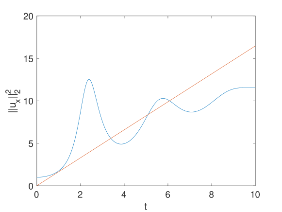
Figure A.1. In blue, the norm $||S_{\alpha}(t)u_{0}||_{H_{1}}^{2}$ for the solution to the equation (1.2) with $\alpha=1$ for the initial data $u_{0}(x)=\frac{{\rm e}^{ix}}{1-p{\rm e}^{ix}}$ with $p=0.5$ in dependence of time. In red, the asymptotic relation (A.2)

The second example studies the case of an initial datum with two poles,

$$u_{0}(x)=\frac{{\rm e}^{ix}}{1-p_{1}{\rm e}^{ix}}+\frac{{\rm e}^{ix}}{1-p_{2}{\rm e}^{ix}},$$

which corresponds to a more complicated phase space than $\mathcal{W}$, but still finite dimensional, since the rank of $K_{u_{0}}$ is $2$. We put $p_{1}=0.7$, $p_{2}=0.8$ and use the same numerical parameters as before. The relative conservation of the momentum is of the order of $10^{-7}$. The norm $||S_{\alpha}(t)u_{0}||_{H_{1}}^{2}$ in dependence of time for this example can be seen in Fig. A.2. The norm appears to grow linearly in time.

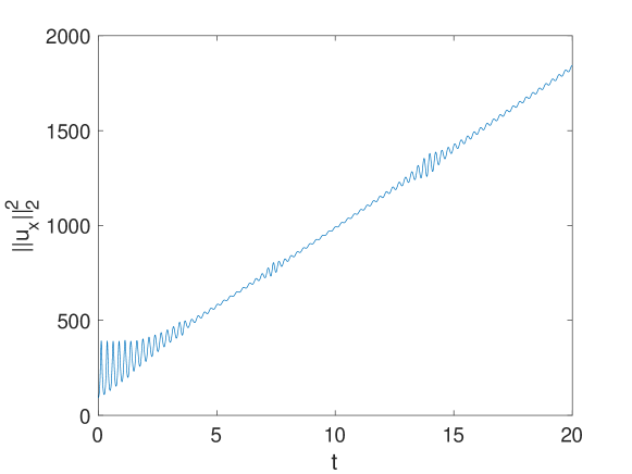
Figure A.2. The norm $||S_{\alpha}(t)u_{0}||_{H_{1}}^{2}$ for the solution to the equation (1.2) with $\alpha=1$ for the initial data $u_{0}(x)=\frac{{\rm e}^{ix}}{1-0.7{\rm e}^{ix}}+\frac{{\rm e}^{ix}}{1-0.8{\rm e}^{ix}}$ in dependence of time.

The third example illustrates the case of an arbitrary initial datum with a Gaussian profile, $u_{0}=\Pi\exp(-10x^{2})$. We use the same numerical parameters, this time for $t\in[0,1000]$. The momentum is conserved to the order of $10^{-13}$. The norm $||S_{\alpha}(t)u_{0}||_{H_{1}}^{2}$ can be seen for this case in Fig. A.3. Once more the square of the $H^{1}$ norm grows linearly in time.

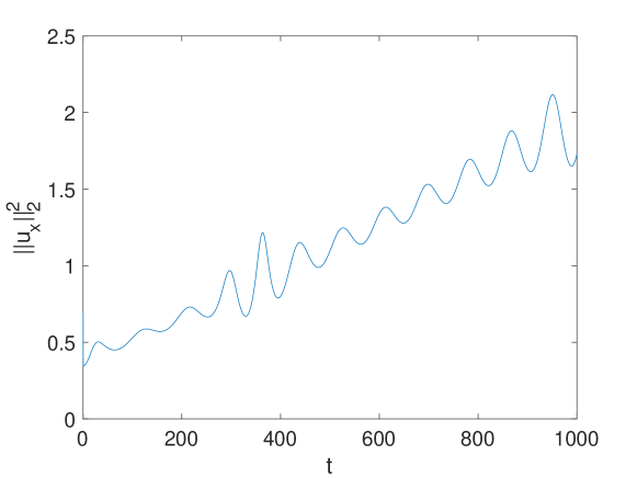
Figure A.3. The norm $||S_{\alpha}(t)u_{0}||_{H_{1}}^{2}$ for the solution to the equation (1.2) with $\alpha=1$ for the initial data $u_{0}(x)=\Pi\exp(-10x^{2})$ in dependence of time.

References

- [1] Bourgain, J., Problems in Hamiltonian PDEs, Geom. Funct. Anal. (2000), Special Volume, Part I, 32–56.
- [2] Bourgain, J., On the growth in time of higher Sobolev norms of smooth solutions of Hamiltonian PDE. Internat. Math. Res. Notices 1996, no. 6, 277–304.
- [3] Carles, R., Gallagher, I., Universal dynamics for the defocusing logarithmic Schrödinger equation , Duke Math. J. 167, (2018), 1761–1801.
- [4] Colliander, J.; Keel, M.; Staffilani, G.; Takaoka, H.; Tao, T. Transfer of energy to high frequencies in the cubic defocusing nonlinear Schrödinger equation. Invent. Math. 181 (2010), no. 1, 39–113.
- [5] Gérard, P., Grellier, S., The cubic Szegő equation, Ann. Scient. Éc. Norm. Sup. 43 (2010), 761–810.
- [6] Gérard, P., Grellier, S., Invariant tori for the cubic Szegő equation, Invent. Math. 187 (2012), 707–754.
- [7] Gérard, P., Grellier, S., The cubic Szegő equation and Hankel operators, Astérisque 389, 2017.
- [8] Gérard, P., Grellier, S., Effective integrable dynamics for a certain nonlinear wave equation, Anal. PDEs 5 (2012), 1139–1155.
- [9] Gérard, P., Wave turbulence and complete integrability, Nonlinear Dispersive Partial Differential Equations and Inverse Scattering, Fields Institute Communications 83, Miller, Perry, Saut, Sulem eds, Springer, to appear.
- [10] Gérard, P., Grellier, S., A survey of the Szegő equation, Science China Mathematics, 62, (2019) 1087–1100.
- [11] Gérard, P., Pushnitski, A., Weighted model spaces and Schmidt subspaces of Hankel operators , J. London Math. Soc. doi: 10.1112/jlms.12270.
- [12] Gérard, P., Lenzmann, E., Pocovnicu, O. Raphael, P. A two-soliton with transient turbulent regime for the cubic half-wave equation on the real line, Annals of PDE. (2018) Springer, 4(7) doi:10.1007/s40818-017-0043-7.
- [13] Guardia, M., Growth of Sobolev norms in the cubic nonlinear Schrödinger equation with a convolution potential. Comm. Math. Phys., 329, (2014), 405–434.
- [14] Guardia, M., Hani, Z., Haus, E., Maspero, A., Procesi, M., Strong nonlinear instability and growth of Sobolev norms near quasiperiodic finite-gap tori for the 2D cubic NLS equation, 45 pages, Preprint available at arXiv:1810.03694 [math.AP].
- [15] Guardia, M., Haus, E., Procesi, M., Growth of Sobolev norms for the defocusing analytic NLS on , Adv. Math., 301, (2016), 615–692.
- [16] Guardia, M., Kaloshin V.,Growth of Sobolev norms in the cubic defocusing nonlinear Schrödinger equation, J. Eur. Math. Soc. (JEMS) 17 (2015), no. 1, 71–149.
- [17] Hani, Z., Long-time strong instability and unbounded orbits for some periodic nonlinear Schrödinger equations, , Archives for Rational Mechanics and Analysis (ARMA) 211 (2014), no. 3, 929–964.
- [18] Hani, Z., Pausader, B., Tzvetkov, N., Visciglia, N., Modified scattering for the cubic Schrödinger equations on product spaces and applications, Forum of Mathematics, Pi. Volume 3 (2015) doi:10.1017/fmp.2015.5.
- [19] Haus, E., Procesi, M., Growth of Sobolev norms for the quintic NLS on , Analysis and PDEs 8 (2015), 883–922.
- [20] Peller, V.V., Hankel Operators and their applications, Springer Monographs in Mathematics. Springer-Verlag, New York, 2003.
- [21] Pocovnicu, O. Explicit formula for the solution of the Szegő equation on the real line and applications, Discrete Cont. Dyn. Syst. 31. (2011), 607–649.
- [22] Thirouin, J., Optimal bounds for the growth of Sobolev norms of solutions of a quadratic Szegő equation , Trans. Amer. Math. Soc. 371 (2019), 3673–3690.
- [23] Xu, H. Large time blow up for a perturbation of the cubic Szegő equation, Anal.PDE. 7 (2014), 717–731.
- [24] Xu, H., Unbounded Sobolev trajectories and modified scattering theory for a wave guide nonlinear Schrödinger equation.Math. Z. 286, (2017), 443–489.