Theory of the special displacement method for
electronic structure calculations at finite temperature

Abstract

Calculations of electronic and optical properties of solids at finite temperature including electron-phonon interactions and quantum zero-point renormalization have enjoyed considerable progress during the past few years. Among the emerging methodologies in this area, we recently proposed a new approach to compute optical spectra at finite temperature including phonon-assisted quantum processes via a single supercell calculation [Zacharias and Giustino, Phys. Rev. B 94, 075125 (2016)]. In the present work we considerably expand the scope of our previous theory starting from a compact reciprocal space formulation, and we demonstrate that this improved approach provides accurate temperature-dependent band structures in three-dimensional and two-dimensional materials, using a special set of atomic displacements in a single supercell calculation. We also demonstrate that our special displacement reproduces the thermal ellipsoids obtained from X-ray crystallography, and yields accurate thermal averages of the mean-square atomic displacements. At a more fundamental level, we show that the special displacement represents an exact single-point approximant of an imaginary-time Feynman’s path integral for the lattice dynamics. This enhanced version of the special displacement method enables non-perturbative, robust, and straightforward ab initio calculations of the electronic and optical properties of solids at finite temperature, and can easily be used as a post-processing step to any electronic structure code. To illustrate the capabilities of this method, we investigate the temperature-dependent band structures and atomic displacement parameters of prototypical nonpolar and polar semiconductors and of a prototypical two-dimensional semiconductor, namely Si, GaAs, and monolayer MoS₂, and we obtain excellent agreement with previous calculations and experiments. Given its simplicity and numerical stability, the present development is suited for high-throughput calculations of band structures, quasiparticle corrections, optical spectra, and transport coefficients at finite temperature.

I Introduction

The calculation of the electronic and optical properties of materials at finite temperature is a long-standing challenge for ab initio electronic structure methods. In typical semiconductors, insulators, metals, and semiconductors, the key mechanism leading to temperature dependent properties is the thermal motion of the atoms in the crystal lattice, and the effect of this motion on the electronic structure of the system. Recent advances have made it possible to study these effects from first principles with predictive accuracy Giustino (2017).

In the case of semiconductors and insulators, one problem that attracted considerable attention during the past decade is the electron-phonon renormalization of band structures, including both quantum zero-point effects and temperature dependence Capaz et al. (2005); Marini (2008); Giustino et al. (2010); Cannuccia and Marini (2011); Gonze et al. (2011); Cannuccia and Marini (2012); Poncé et al. (2014a); Kawai et al. (2014); Antonius et al. (2014); Poncé et al. (2014b, 2015); Antonius et al. (2015); Molina-Sánchez et al. (2016); Monserrat and Needs (2014); Engel et al. (2015); Lloyd-Williams and Monserrat (2015); Patrick et al. (2015); Monserrat (2016a, b); Nery and Allen (2016a); Allen and Nery (2017); Karsai et al. (2018a). This problem is becoming increasingly important as we strive to achieve close quantitative agreement between ab initio calculations and experimental data. Furthermore this problem underpins calculations of many important properties, from temperature-dependent optical absorption Noffsinger et al. (2012); Zacharias et al. (2015); Zacharias and Giustino (2016) and emission spectra Paleari et al. (2019) to temperature-dependent transport coefficients Gunst et al. (2017); Palsgaard et al. (2018).

The calculation of temperature-dependent electronic and optical properties has been demonstrated using both perturbative approaches based on density functional perturbation theory Baroni et al. (2001) (DFPT) calculations in the crystal unit cell, and non-perturbative approaches based on density functional theory (DFT) calculations in large supercells. In perturbative methods the key ingredient of the calculations is the electron-phonon matrix element, that is the scattering matrix element between two Kohn-Sham states which results from the variation of the self-consistent potential associated with a vibrational eigenmode. The matrix elements are employed to obtain temperature-dependent band structures in the Allen-Heine (AH) method Allen and Heine (1976); Allen and Cardona (1981), and to compute indirect optical absorption in the Hall, Bardeen, and Blatt theory Hall et al. (1954); Bassani and Parravicini (1975). These approaches have enjoyed considerable success during the past decade across a broad range of materials Marini (2008); Giustino et al. (2010); Cannuccia and Marini (2011, 2012); Noffsinger et al. (2012); Antonius et al. (2014); Poncé et al. (2014b, a); Kawai et al. (2014); Antonius et al. (2015); Poncé et al. (2015); Molina-Sánchez et al. (2016); Saidi et al. (2016); Menéndez et al. (2017); Ge et al. ; Querales-Flores et al. (2019).

Non-perturbative supercell-based methods offer an alternative approach to calculations of electronic and optical properties at finite temperature. The central idea of these methods is that the interactions between electrons and phonons can be described using large supercells where the atoms are displaced to capture thermal disorder Monserrat (2018). Supercell methods derive from earlier frozen-phonon approaches Chang and Cohen (1986); Capaz et al. (2005), and do not require the explicit evaluation of electron-phonon matrix elements. In order to sample thermal disorder, the first attempts in this area relied on the Monte Carlo sampling of quantum nuclear wavefunctions, either in the atomic configuration space Patrick and Giustino (2013, 2014); Zacharias et al. (2015) or in the space of normal vibrational modes Monserrat (2016a, b); Bravić and Monserrat (2019). The formal basis for this approach is provided by a theory developed in the 1950s by Williams Williams (1951) and Lax Lax (1952) to study defects in solids, and recently extended by Zacharias et al. to finite-temperature optical spectra, phonon-assisted optical processes, and band gap renormalization Zacharias et al. (2015).

The central idea behind Monte Carlo supercell methods is that the temperature dependence of the dielectric function $\epsilon(\omega;T)$ results from a multivariate Gaussian integral given by Zacharias and Giustino (2016):

$$\epsilon(\omega;T)=\prod_{\nu}\int x_{\nu}\frac{\text{exp}(-x^{2}_{\nu}/2\sigma^{2}_{\nu,T})}{\sqrt{2\pi}\sigma_{\nu,T}}\epsilon(\omega;x)$$ (1)

where the product runs over the normal coordinates $x_{\nu}$, and each width $\sigma_{\nu,T}$ of the independent Gaussians represents the root mean square displacement of the atoms at temperature $T$ along a phonon mode $\nu$. The interpretation of Eq. (1) is that the temperature dependence of the spectrum can directly be obtained as an ensemble average over the spectra calculated at fixed nuclear coordinates $x$, whose probability density function is a multivariate Gaussian.

The disadvantages of stochastic supercell approaches are that (i) it is difficult to control the rate of convergence with the number of random samples, and (ii) the final outcome of the calculations is a distribution of values at each temperature, e.g. band gaps, rather than a unique value as in perturbative methods. Furthermore, performing stochastic sampling on large supercells can be prohibitively costly from the computational standpoint. In order to overcome these limitations, in Ref. [Zacharias and Giustino, 2016] we demonstrated that it is possible to replace the stochastic sampling of the nuclear wavefunctions by a single supercell calculation with a precise choice of atomic displacements. The possibility of studying electronic and optical spectra at finite temperature using a single supercell calculation enabled several interesting applications. For example, in Ref. [Zacharias and Giustino, 2016] we reported temperature-dependent phonon-assisted optical spectra of Si, diamond, and GaAs based on this method; Refs. [Biswas et al., 2017], [Zhang et al., 2018] and [Kang et al., 2018] applied this method to the dielectric function of Zn₂Mo₃O₈, metallic hydrogen, and BaSnO₃, respectively; Ref. [Karsai et al., 2018a] used this technique to compute GW quasiparticle band gaps at finite temperature for diamond, BN, SiC, Si, AlP, ZnO, GaN, ZnS, GaP, AlAs, ZnSe, CdS, GaAs, Ge, AlSb, CdSe, ZnTe, and CdTe; Ref. [Karsai et al., 2018b] calculated exciton-phonon couplings in hexagonal boron nitride; and Refs. [Gunst et al., 2017, Palsgaard et al., 2018] demonstrated calculations of finite-temperature carrier mobilities in silicon $n$-i-$n$ and $p$-$n$ junctions using this approach. In retrospect, these successes across a broad range of applications are not too surprising, since the method of Ref. [Zacharias and Giustino, 2016] is designed to provide, in the limit of large supercell, the exact thermodynamic average of any property that can be expressed in the form of Fermi’s golden rule: this includes in principle photoelectron spectra (hence band gaps and band structures), optical spectra, tunneling spectra, and transport coefficients.

One potential limitation of Ref. [Zacharias and Giustino, 2016] is that the theory was developed using a $\Gamma$-point formalism, therefore phonon calculations to determine the vibrational eigenmodes in the supercell are demanding. Furthermore, by addressing only $\Gamma$-point properties, the calculations are limited to angle-integrated spectra, such as density-of-states (DOS) and optical absorption spectra. Finally, it has been pointed out that the choice of the special displacement employed in Ref. [Zacharias and Giustino, 2016] might be improved to reduce the size of the supercell required to achieve convergence Karsai et al. (2018a).

In this manuscript, we significantly expand the scope of the methodology introduced in Ref. [Zacharias and Giustino, 2016] by formulating the theory within a compact reciprocal space formulation, and exploiting translational invariance and time-reversal symmetry. This upgrade allows us to determine the special supercell displacement using quantities that are computed in a crystal unit cell via DFPT. In a nutshell, we demonstrate that a supercell calculation where the atoms are displaced according to:

$$\Delta{\bm{\tau}}_{p\kappa} = \!\sum_{{\bf q}\in\mathcal{B},\nu}\!S_{{\bf q}\nu}\left[\!\frac{\hbar}{2N_{p}M_{\kappa}\omega_{{\bf q}\nu}}(2n_{{\bf q}\nu,T}+1)\!\right]^{\!\frac{1}{2}}$$ (2)

$$\times 2\,{\rm Re}\Big{[}e^{i{\bf q}\cdot{\bf R}_{p}}{\bf e}_{\kappa,\nu}({\bf q})\Big{]}.$$

yields the exact thermodynamic average of electronic and optical properties at the temperature $T$ in the adiabatic and harmonic approximations. In the above expressions $\Delta{\bm{\tau}}_{p\kappa}$ indicates the displacement of the atom $\kappa$ with mass $M_{\kappa}$ in the unit cell with lattice vector ${\bf R}_{p}$, and $N_{p}$ is the number of unit cells in the supercell. ${\bf e}_{\kappa,\nu}({\bf q})$ is the phonon polarization vector of the normal mode (normalized within the unit cell) with wavevector ${\bf q}$, branch index $\nu$, frequency $\omega_{{\bf q}\nu}$, and Bose-Einstein occupation $n_{{\bf q}\nu,T}$. The quantities $S_{{\bf q}\nu}$ are signs, $+$ or $-$, which depend on the normal mode, as specified in Sec. V. The summation is restricted to phonon wavevectors that are not time-reversal partners. In particular, we define this group of phonons as set $\mathcal{B}$. The real part in the equation arises from grouping together a phonon with wavevector ${\bf q}\in\mathcal{B}$ and its partner $-{\bf q}$. Phonon wavevectors that coincide with their time-reversal partners are grouped in a finite set $\mathcal{A}$, and their contribution to the atomic displacements vanishes in the limit of dense Brillouin-zone sampling. This partitioning is discussed in greater detail in Sec. II.

Equation (2) reduces to our previous prescription provided in Ref. [Zacharias and Giustino, 2016] if we perform $\Gamma$-point sampling, but is much more powerful since the construction of the special displacement relies on DFPT calculations in the unit cell. Therefore the only expensive step is one calculation of the desired property in a large supercell. To demonstrate the power of this approach, we report for the first time complete temperature-dependent band structures based on Eq. (2) for both three-dimensional semiconductors, Si and GaAs, and two-dimensional semiconductors (MoS₂), and we show that this method delivers an accuracy comparable to perturbative techniques, without requiring the so-called rigid-ion approximation of the Debye-Waller self-energy Poncé et al. (2015); Molina-Sánchez et al. (2016). We also demonstrate that Eq. (2) is an exact single-point approximant to an imaginary-time path integral in the space of nuclear configurations, and that it reproduces very accurately the thermal displacement ellipsoids measured by X-ray diffraction (XRD).

The method of Ref. [Zacharias and Giustino, 2016] was originally named ‘one-shot configuration’, but subsequently it has variably been referred to as the ‘WL-HA’ method Zhang et al. (2018) or the ‘STD’ method Gunst et al. (2017). In order to avoid a proliferation of acronyms, in this manuscript we will refer to the general theory as the special displacement method (SDM), and to Eq. (2) as the ZG displacement.

The manuscript is organized as follows. In Sec. II we describe the Williams-Lax theory that underpins our method, and we write the key equations using a reciprocal-space formulation. In Sec. III we establish the connection between the ZG displacement and thermal ellipsoids. In Sec. IV we show that the Williams-Lax theory can be recast in the form of an imaginary-time Feynman’s path integral, and that the ZG displacement enables an efficient single-point evaluation of this path integral. Section V is devoted to the construction of the ZG displacement and the determination of the mode signs $S_{{\bf q}\nu}$ in Eq. (2). In Sec. VI we provide all computational details of the present calculations, including the unfolding of bands and spectral functions. In Sec. VII we briefly outline the procedure that we follow to determine the ZG displacement, and we demonstrate our main computational results. We show the temperature-dependent thermal ellipsoids, band structures and band gaps of Si, GaAs, and monolayer MoS₂ using the SDM. Here we also provide detailed convergence tests and show that accurate results can be obtained even with relatively small supercells. In Sec. VIII we summarize our key findings and discuss future directions. More technical aspects are left to the Appendices.

II The Williams-Lax theory

II.1 General remarks

The theoretical framework underlying our present methodology was laid out in two works by Williams Williams (1951) and Lax Lax (1952) in the 1950s, which we refer to collectively as the Williams-Lax theory. This theory starts from the Herzberg-Teller rate Herzberg (1966); Patrick and Giustino (2014) that describes transitions between coupled electron-phonon states driven by an external field, and replaces the final quantum nuclear states by a semiclassical continuum. Formally this step corresponds to neglecting commutators involving the nuclear kinetic energy operator, and is related (albeit not identical) to the adiabatic Born-Oppenheimer approximation Patrick and Giustino (2014). This approach is also closely related to Feynman path integrals Feynman and Hibbs (1965), as we discuss in detail in Sec. IV.

If we denote a Born-Oppenheimer quantum state using the ket $|\alpha n\rangle$, with the Greek letter referring to the electronic part and the integer to the nuclear part Patrick and Giustino (2014), then the Williams-Lax theory provides a semiclassical approximation for the transition rate from an initial state $|\alpha n\rangle$ to all final states $|\beta m\rangle$ with the same $\beta$ and every possible vibrational state $m$, evaluated using Fermi’s golden rule:

$$\Gamma_{\alpha n\rightarrow\beta}(\omega)=\!\!\int\!d\tau|\chi_{\alpha n}(\{\tau\})|^{2}\,\Gamma_{\alpha\rightarrow\beta}^{\{\tau\}}(\omega).$$ (3)

In this expression $\omega$ is the frequency of the driving external field, the $\chi_{\alpha n}(\{\tau\})$ are the quantum nuclear wavefunctions for the potential energy surface associated with the electronic state $\alpha$, and $\{\tau\}$ denotes the set of all atomic coordinates. $\Gamma_{\alpha\rightarrow\beta}^{\{\tau\}}(\omega)$ is the transition rate evaluated with the atoms clamped in the positions ${\{\tau\}}$:

$$\Gamma_{{\alpha}\rightarrow\beta}^{\{\tau\}}(\omega)=\frac{2\pi}{\hbar}|M^{\{\tau\}}_{{\alpha}\rightarrow\beta}|^{2}\delta\left(E^{\{\tau\}}_{\beta}-E^{\{\tau\}}_{{\alpha}}-\hbar\omega\right),$$ (4)

where $E^{\{\tau\}}_{\alpha}$, $E^{\{\tau\}}_{\beta}$, and $M^{\{\tau\}}_{{\alpha}\rightarrow\beta}$ denote the energies of the initial and final electronic states and the associated transition matrix elements, respectively, all evaluated at clamped atoms. For example $\Gamma_{\alpha\rightarrow\beta}^{\{\tau\}}(\omega)$ can represent the optical transition rates for light absorption, or the charge current in electron tunneling. Equation (3) formalizes the intuitive concept that the transition rate including quantum nuclear effects can be obtained by averaging ‘static’ clamped-ion rates over the nuclear probability distributions $|\chi_{\alpha n}(\{\tau\})|^{2}$ of the initial state.

The transition rate at a finite temperature $T$ is obtained from Eq. (3) by carrying out a canonical average over the vibrational quantum numbers of the initial state Lax (1952); Patrick and Giustino (2014); Zacharias and Giustino (2016):

$$\Gamma_{\alpha\rightarrow\beta}(\omega,T)=\frac{1}{Z}\sum_{n}\exp(-E_{\alpha n}/k_{\rm B}T)\,\Gamma_{\alpha n\rightarrow\beta}(\omega),$$ (5)

where $k_{\rm B}$ stands for the Boltzmann constant and $Z=\sum_{n}\exp(-E_{\alpha n}/k_{\rm B}T)$ is the canonical partition function. Here $E_{\alpha n}$ denotes the vibrational energy of the state $|\alpha n\rangle$. This approach has been used in a number of investigations and is well established by now Williams (1951); Lax (1952); Della Sala et al. (2004); Patrick and Giustino (2014); Zacharias et al. (2015); Zacharias and Giustino (2016); Biswas et al. (2017); Monserrat et al. (2018); Morris and Monserrat (2018); Karsai et al. (2018a).

Since Eqs. (3)-(5) involve the calculations of transition rates for displaced atomic configurations $\{\tau\}$, the results automatically incorporate the effect of electron-phonon couplings, because the method probes the change in the electronic energies and wavefunctions upon displacing the atoms. We emphasize that Eqs. (3)-(5) apply to any property that can be obtained from the Fermi golden rule, in particular optical spectra, photoemission spectra, transport coefficients, and tunneling spectra. Furthermore, these equations provide the formal basis for computing temperature-dependent electronic eigenvalues. Indeed, if we consider transitions from an electronic state $|\alpha n\rangle$ of a solid into free electron states, as in photoemission experiments, the final free electron states are independent of atomic positions, therefore the first frequency moment of the transition rates, $\int d\omega\,\omega\,\Gamma_{\alpha\rightarrow\beta}(\omega,T)$, yields the temperature-dependent electronic energy of the initial state:

$$E_{\alpha}(T)=\frac{1}{Z}\sum_{n}\exp(-E_{\alpha n}/k_{\rm B}T)\int d\tau|X_{\alpha n}(\{\tau\})|^{2}E^{\{\tau\}}_{\alpha}.$$ (6)

This relation states that, in the Williams-Lax theory, the temperature-dependent electronic energy $E_{\alpha}(T)$ can be obtained by averaging the position-dependent energy $E^{\{\tau\}}_{\alpha}$ over thermal fluctuations. This observation forms the basis for all non-perturbative supercell calculations of temperature-dependent electronic properties, and is also at the basis of the adiabatic formulation of the Allen-Heine theory of temperature-dependent band structures Allen and Heine (1976).

An important implication of Eq. (6) is that, if we describe ions classically, then $E_{\alpha}(T)$ corresponds to averaging electronic energies over the snapshots of a molecular dynamics trajectory. This concept has been used extensively in the literature, but to the best of our knowledge the connection to the Williams-Lax theory is still not fully appreciated.

II.2 Reciprocal space formulation

In this section we recast Eqs. (3)-(5) in a language appropriate for ab initio calculations in periodic crystals. From now on we assume the harmonic approximation, so that we can define phonons in the usual way. We employ the same standard notation as in Ref. [Giustino, 2017], and we choose the convention for the phase of vibrational eigenmodes as in Ref. [Maradudin and Vosko, 1968].

We consider a Born-von Kármán supercell containing $N_{p}$ unit cells with $M$ atoms each. The position vector of the atom $\kappa$ in the unit cell $p$ at zero temperature is ${\boldsymbol{\tau}}_{\kappa p}={\bf R}_{p}+{\boldsymbol{\tau}}_{\kappa}$, where ${\bf R}_{p}$ indicates a direct lattice vector, and ${\bm{\tau}}_{\kappa}$ is the position vector in the primitive unit cell, with Cartesian components $\tau_{p\kappa\alpha}$. The atomic displacements from equilibrium are written as a linear combination of normal vibrational modes Giustino (2017):

$$\Delta\tau_{p\kappa{\alpha}}=N_{p}^{-1/2}\bigg{(}\frac{M_{0}}{M_{\kappa}}\bigg{)}^{1/2}\sum_{{\bf q}\nu}e^{i{\bf q}\cdot{\bf R}_{p}}e_{\kappa{\alpha},\nu}({\bf q})\,z_{{\bf q}\nu},$$ (7)

where the $z_{{\bf q}\nu}$ are the complex-valued normal coordinates Peter (1982). The inverse relation is:

$$z_{{\bf q}\nu}=N_{p}^{-1/2}\sum_{p\kappa{\alpha}}\bigg{(}\frac{M_{\kappa}}{M_{0}}\bigg{)}^{1/2}e^{-i{\bf q}\cdot{\bf R}_{p}}e^{*}_{\kappa{\alpha},\nu}({\bf q})\,\Delta\tau_{p\kappa{\alpha}}\,.$$ (8)

In both equations $M_{0}$ is an arbitrary reference mass, usually chosen to be the proton mass, and the summations run over all the $3MN_{p}$ atomic degrees of freedom. For completeness, in Appendix A we give the standard textbook relations between normal modes.

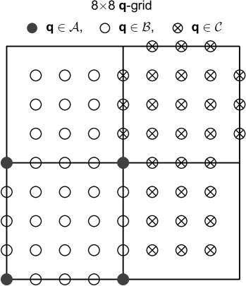
Figure 1: Partition of the Brillouin zone grid in sets $\mathcal{A}$, $\mathcal{B}$, and $\mathcal{C}$. Shown is an 8$\times$8 two-dimensional $\Gamma$-centered grid. Wavevectors which are invariant with respect to time-reversal $-{\bf q}={\bf q}+{\bf G}$ belong to set $\mathcal{A}$ (filled disks), The other wavevectors are separated into a set $\mathcal{B}$ which does not contain the time-reversal partner of any element (empty circles), and set $\mathcal{C}$ obtained by reversing the sign of the wavevectors in set $\mathcal{B}$ (crossed empty circles).

If we write $z_{{\bf q}\nu}=x_{{\bf q}\nu}+iy_{{\bf q}\nu}$, with $x_{{\bf q}\nu}$ and $y_{{\bf q}\nu}$ being the real normal coordinates, Eq. (8) and time-reversal symmetry imply $x_{-{\bf q}\nu}=x_{{\bf q}\nu}$ and $y_{-{\bf q}\nu}=-y_{{\bf q}\nu}$. Therefore only half of the real normal coordinates are independent. The wavevectors ${\bf q}$ of these independent coordinates occupy half of the first Brillouin zone. This is illustrated in Fig. 1, where we consider a regular ${\bf q}$-grids of size 8$\times$8. This grid can be partitioned in three sets, $\mathcal{A}$, $\mathcal{B}$, and $\mathcal{C}$, following Appendix B of Ref. [Giustino, 2017]. Set $\mathcal{A}$ includes the ${\bf q}$-points that are invariant under inversion, modulo a reciprocal lattice vector. Therefore the ${\bf q}$-points in this set correspond to the center of the Brillouin zone, the centers of its faces, and the corners, as shown by the filled disks in Fig. 1. Set $\mathcal{B}$ includes all the ${\bf q}$-points that are not inversion partners (modulo a reciprocal lattice vector), as shown by the empty circles in Fig. 1. Set $\mathcal{C}$ is obtained by changing the sign of all the points in $\mathcal{B}$, and is denoted by crossed filled circles in Fig. 1. Using this partitioning we can write the atomic displacements in terms of independent real normal coordinates as:

$$\Delta\tau_{p\kappa{\alpha}} = N_{p}^{-1/2}\bigg{(}\frac{M_{0}}{M_{\kappa}}\bigg{)}^{1/2}\Bigg{[}\sum_{{\bf q}\in\mathcal{A},\nu}e_{\kappa{\alpha},\nu}({\bf q})x_{{\bf q}\nu}\text{cos}({\bf q}\cdot{\bf R}_{p})$$ (9)

$$+ 2\hskip 0.5pt{\rm Re}\!\!\sum_{{\bf q}\in\mathcal{B},\nu}e^{i{\bf q}\cdot{\bf R}_{p}}e_{\kappa{\alpha},\nu}({\bf q})(x_{{\bf q}\nu}+iy_{{\bf q}\nu})\Bigg{]}.$$

Equation (9) allows us to write the total quantum nuclear wavefunction of the state $|\alpha n\rangle$ in the harmonic approximation Ziman (1960):

$$\chi_{n}(\{{\bm{\tau}}_{p\kappa}+\Delta{\bm{\tau}}_{p\kappa}\})=$$

$$\hskip 40.0pt\prod_{{\bf q}\in A,\nu}\!\!\chi_{n_{{\bf q}\nu}}(x_{{\bf q}\nu})\!\!\prod_{{\bf q}\in\mathcal{B},\nu}\!\!\chi_{n_{{\bf q}\nu}}(x_{{\bf q}\nu})\chi_{n_{{\bf q}\nu}}(y_{{\bf q}\nu}).$$ (10)

Here we omitted the subscript $\alpha$ for notational simplicity. $\chi_{n_{{\bf q}\nu}}(x)$ represents the wavefunction of a quantum harmonic oscillator with frequency $\omega_{{\bf q}\nu}$ and quantum number $n_{{\bf q}\nu}$; in particular, for ${\bf q}\in\mathcal{A}$ we have:

$$\chi_{n_{{\bf q}\nu}}(x)=\frac{(4\pi l_{{\bf q}\nu}^{2})^{-1/4}}{\sqrt{2^{n_{{\bf q}\nu}}n_{{\bf q}\nu}!\ }}e^{-x^{2}/8l_{{\bf q}\nu}^{2}}H_{n_{{\bf q}\nu}}(x/2l_{{\bf q}\nu}),$$ (11)

while for ${\bf q}\in\mathcal{B}$ we have:

$$\chi_{n_{{\bf q}\nu}}(x)=\frac{(\pi l_{{\bf q}\nu}^{2})^{-1/4}}{\sqrt{2^{n_{{\bf q}\nu}}n_{{\bf q}\nu}!\ }}e^{-x_{{\bf q}\nu}^{2}/2l_{{\bf q}\nu}^{2}}H_{n_{{\bf q}\nu}}(x/l_{{\bf q}\nu}).$$ (12)

Here $l_{{\bf q}\nu}=(\hbar/2M_{0}\omega_{{\bf q}\nu})^{1/2}$ is the zero-point vibrational amplitude, and $H_{m}(x)$ denotes the Hermite polynomial of order $m$. The total energy of the state $\chi_{n}$ is given by the standard expression:

$$E_{n}=\sum_{{\bf q}\nu}(n_{{\bf q}\nu}+1/2)\hbar\omega_{{\bf q}\nu}.$$ (13)

By substituting Eqs. (II.2)-(13) inside Eqs. (3) and (5), and using Mehler’s sum rule for Hermite functions Watson (1933), we obtain the compact expression Patrick and Giustino (2014):

$$\Gamma_{\alpha\rightarrow\beta}(\omega,T)=\prod_{{\bf q}\in\mathcal{A},\nu}\!\int\!\frac{dx_{{\bf q}\nu}}{2\sqrt{\pi}\sigma_{{\bf q}\nu}}e^{-\frac{x^{2}_{{\bf q}\nu}}{4\sigma^{2}_{{\bf q}\nu}}}$$

$$\quad\times\!\!\!\prod_{{\bf q}\in\mathcal{B},\nu}\!\int\!\frac{dx_{{\bf q}\nu}dy_{{\bf q}\nu}}{\pi\sigma^{2}_{{\bf q}\nu}}e^{-\frac{(x^{2}_{{\bf q}\nu}+y^{2}_{{\bf q}\nu})}{\sigma^{2}_{{\bf q}\nu}}}\Gamma_{\alpha\rightarrow\beta}^{\{x_{{\bf q}\nu},y_{{\bf q}\nu}\}}(\omega),\hskip 10.0pt$$ (14)

where $\sigma_{{\bf q}\nu}$ is the mean square displacement of the normal mode at the temperature $T$ and is given by:

$$\sigma^{2}_{{\bf q}\nu}=l^{2}_{{\bf q}\nu}(2n_{{\bf q}\nu,T}+1).$$ (15)

Here $n_{{\bf q}\nu,T}=[{\rm exp}(\hbar\omega_{{\bf q}\nu}/k_{\rm B}T)-1]^{-1}$ is the Bose-Einstein occupation of the mode with frequency $\omega_{{\bf q}\nu}$.

Equation (II.2) states that the temperature-dependent transition rate $\Gamma_{\alpha\rightarrow\beta}(\omega,T)$ is obtained by averaging the transition rates calculated at clamped atoms for a variety of atomic configurations specified by the normal coordinates $\{x_{{\bf q}\nu},y_{{\bf q}\nu}\}$, and that the average is to be taken using a multidimensional Gaussian importance function. In this context the temperature $T$ sets the width of each Gaussian via Eq. (15). As a sanity check, we note that if $\Gamma_{\alpha\rightarrow\beta}^{\{\tau\}}(\omega)$ does not depend on the atomic coordinates, Eq. (II.2) yields the correct temperature-independent rate.

The core of the special displacement method described in this manuscript is to identify one set of atomic displacements so that a single evaluation of $\Gamma_{\alpha\rightarrow\beta}^{\{x_{{\bf q}\nu},y_{{\bf q}\nu}\}}(\omega)$ yields the same result as the multidimensional integral in Eq. (II.2). From this perspective, the task of finding the ZG displacement is similar to finding the mean value point of a definite integral; the only difference is that we are dealing with a multi-dimensional integral with hundreds to thousands of variables.

III ZG displacement and thermal ellipsoids

In this section we discuss the physical meaning of the ZG displacement in Eq. (2). In particular we prove rigorously that the ZG displacement reproduces the displacement autocorrelation function obtained from the quantum canonical average Kittel (1976), and therefore encodes information about the thermal ellipsoids measured via XRD. Furthermore, using explicit calculations, we demonstrate that the ZG displacement yields the correct thermal distribution of the atomic coordinates to all orders.

When a harmonic crystal is in thermodynamic equilibrium at the temperature $T$, the atomic displacements $\Delta\tau_{p\kappa{\alpha}}$ follow a normal distribution. This a direct consequence of the fact that the marginal distribution of a multivariate normal is also normal. In particular we have (cf. Eq. 7.2.21 of Ref. [Maradudin et al., 1963]):

$$P(\Delta\tau_{p\kappa{\alpha}};T)=\frac{1}{\sqrt{2\pi}\sigma_{\kappa{\alpha}}(T)}\text{exp}\left[-\frac{\Delta\tau_{p\kappa{\alpha}}^{2}}{2\sigma^{2}_{\kappa{\alpha}}(T)}\right],$$ (16)

where the width $\sigma_{\kappa{\alpha}}(T)$ of the Gaussian is given by (cf. Eq. 7.2.5 of Ref. [Maradudin et al., 1963]):

$$\sigma^{2}_{\kappa{\alpha}}(T)=\frac{2}{N_{p}}\sum_{{\bf q}\in\mathcal{B},\nu}|e_{\kappa{\alpha},\nu}({\bf q})|^{2}\frac{\hbar}{2M_{\kappa}\omega_{{\bf q}\nu}}(2n_{{\bf q}\nu,T}+1).$$ (17)

Here the limit of dense Brillouin-zone sampling is implied; in this limit the contribution to the sum of phonons with ${\bf q}\in\mathcal{A}$ vanishes. The width $\sigma_{\kappa{\alpha}}(T)$ is a particular case of the tensor of anisotropic displacement parameters (ADPs), defined as Trueblood et al. (1996):

$$U_{\kappa,{\alpha}{\beta}}(T)=\langle\Delta\tau_{p\kappa{\alpha}}\Delta\tau_{p\kappa{\beta}}\rangle_{T},$$ (18)

where $\langle\cdot\rangle_{T}$ denotes the canonical average over vibrational quantum states. In fact, by combining Eqs. (18) and (16) it follows directly that $\sigma^{2}_{\kappa{\alpha}}(T)=U_{\kappa,{\alpha}{\alpha}}(T)$. The ADPs of Eq. (18) are the values employed to generate thermal ellipsoids when visualizing crystal structures at finite temperature.

If we start from the ZG displacement, and we take the mean square displacement of the atom $\kappa$ over all the unit cells of the supercell, then we obtain precisely the thermodynamic average given by Eq. (17). In fact, by replacing the ZG displacement of Eq. (2) inside the sum $\sum_{p}\Delta\tau_{p\kappa{\alpha}}^{2}/N_{p}$, and using the sum rule in Eq. (72), we find immediately:

$$\frac{1}{N_{p}}\!\sum_{p}\Delta\tau_{p\kappa{\alpha}}^{2}\!=\frac{2}{N_{p}}\!\sum_{{\bf q}\in\mathcal{B},\nu}\!|e_{\kappa{\alpha},\nu}({\bf q})|^{2}\frac{\hbar}{2M_{\kappa}\omega_{{\bf q}\nu}}(2n_{{\bf q}\nu,T}+1)$$

$$\,\,+\frac{2}{N_{p}}\frac{M_{0}}{M_{\kappa}}\sum_{{\bf q}\in\mathcal{B}}^{\nu\neq\nu^{\prime}}S_{{\bf q}\nu}S_{{\bf q}\nu^{\prime}}\hskip 0.5pt{\rm Re}[e_{\kappa{\alpha},\nu}({\bf q})e^{*}_{\kappa{\alpha},\nu^{\prime}}({\bf q})]\sigma_{{\bf q}\nu}\sigma_{{\bf q}\nu^{\prime}}$$

$$\,\,+\frac{1}{N_{p}}\sum_{{\bf q}\in\mathcal{A}}\left[\cdots\right].$$ (19)

The third line contains terms associated with ${\bf q}\in\mathcal{A}$ phonons. As we prove below in Sec. V.4, all contributions arising from ${\bf q}\in\mathcal{A}$ phonons vanish in the limit of large supercell. Furthermore, the choice of signs $S_{{\bf q}\nu}$ in the ZG displacement guarantees that also the second line of Eq. (III) vanishes in the thermodynamic limit. Therefore in this limit we recover precisely the mean-square displacements $\sigma^{2}_{\kappa{\alpha}}(T)$ of Eq. (17).

In Sec. VII.1 we show that these results are confirmed by explicit calculations on Si, GaAs, and MoS₂.

IV The ZG displacement and Feynman’s path integrals

An important property of the ZG displacement is that it can be understood as an exact single-point approximant to a Feynman’s path integral Feynman and Hibbs (1965).

In path integral approaches, such as path integral Monte Carlo simulations Weht et al. (1998); Della Sala et al. (2004); Tuckerman (2010) and path integral molecular dynamics Ramírez et al. (2006); Zhang et al. (2018); Marx and Hutter (2009), the electronic and ionic degrees of freedom are decoupled using the adiabatic approximation, and the quantum nature of the atomic nuclei is taken into account by averaging the electronic properties over all possible trajectories of the atomic nuclei. In order to obtain the correct quantum statistics, each trajectory is weighted by $\exp(-S_{\rm E}/\hbar)$, where $S_{\rm E}$ is the Euclidean action associated with a path Feynman and Hibbs (1965), and is defined in Eq. (22) below.

We now show that the Williams-Lax rate can be recast exactly in the language of path integrals. The equivalence between the two approaches was originally identified in Ref. [Della Sala et al., 2004]. By combining Eqs. (5) and (3) and using the relations $\chi_{{\alpha}n}(\{\tau\})=\langle\tau|{\alpha}n\rangle$, $\sum_{n}\ket{{\alpha}n}\bra{{\alpha}n}=1$, and $\hat{H}_{\rm n}\ket{{\alpha}n}=E_{{\alpha}n}\ket{{\alpha}n}$, we find:

$$\Gamma_{{\alpha}\rightarrow\beta}(\omega;T)=\frac{1}{Z}\int d\tau\braket{\tau}{e^{-\hat{H}_{\rm n}/k_{\rm B}T}}{\tau}\Gamma_{{\alpha}\rightarrow\beta}^{\{\tau\}}(\omega).$$ (20)

In these expressions $\ket{\tau}$ represents position eigenstates for all atomic coordinates, and $\hat{H}_{\rm n}$ is the nuclear Hamiltonian for the adiabatic potential energy surface $E_{\alpha}^{\{\tau\}}$.

Now by combining together Eqs. (74)-(77), the Williams-Lax transition rate assumes the form of a thermodynamic Feynman path integral Feynman and Hibbs (1965); Della Sala et al. (2004); Tuckerman (2010); Zhang et al. (2018):

$$\Gamma_{{\alpha}\rightarrow\beta}(\omega;T) = \frac{1}{Z_{\rm F}}\int d\tau\,\Gamma_{{\alpha}\rightarrow\beta}^{\{\tau\}}(\omega)$$

$$\times \int_{\tau^{\prime}(0)=\tau}^{\tau^{\prime}(\hbar/k_{\rm B}T)=\tau}\mathcal{D}\tau^{\prime}{\rm exp}\bigg{(}-\frac{1}{\hbar}S_{E}[\tau^{\prime}]\bigg{)},$$

where the notation $\int_{\tau^{\prime}(0)=\tau}^{\tau^{\prime}(k_{\rm B}T)=\tau}\mathcal{D}\tau^{\prime}$ indicates the sum over all paths that begin from the set of atomic coordinates $\{\tau\}$ at the time $t=0$ and go back to the same initial coordinates at the time $t=\hbar/k_{\rm B}T$. $S_{\rm E}$ is the Euclidean action evaluated along each one of these paths:

$$S_{E}=\int_{0}^{\hbar/k_{\rm B}T}\!\left[\,\sum_{p\kappa{\alpha}}\frac{1}{2}M_{\kappa}\dot{\tau}_{p\kappa{\alpha}}^{2}+U_{\alpha}(\{\tau\})\right]dt,$$ (22)

where $\dot{\tau}_{p\kappa{\alpha}}$ represents the classical velocities of the nuclei and $U_{\alpha}$ is the potential energy of the nuclear Hamiltonian. The partition function $Z_{\rm F}$ is equal to the second line of Eq. (IV).

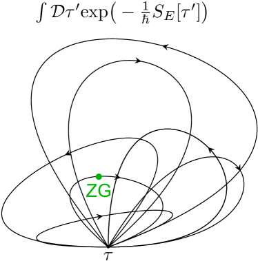
Figure 2: Schematic representation of closed-loop paths required to evaluate the finite-temperature electronic and optical properties using thermodynamic Feynman’s path integrals. The Williams-Lax theory is equivalent to averaging the property of interest over many atomic configuration $\{\tau\}$. The weight of each configuration is given by the the sum of all possible path integrals starting and ending with the configuration $\{\tau\}$. The special displacement method replaces the average over paths by a single evaluation of the property using the ZG displacement (green disk).

Equation (IV) states that the Williams-Lax transition rates can be obtained by averaging the electronic transitions at clamped ions using thermodynamic path integrals as weighting coefficients. For each atomic configuration ‘snapshot’ $\{\tau\}$, we must evaluate all closed-loop path integrals that begin and terminate at $\{\tau\}$, see Fig. 2. At high temperature, $k_{\rm B}T\gg\hbar\omega$ (with $\omega$ being the highest vibrational frequency), Eq. (IV) assigns the largest weights to paths that minimize the classical action, therefore the William-Lax theory reduces to a standard configurational average using classical Boltzmann weights. Based on these observations, we can regard Eq. (IV) as the link between the Williams-Lax theory, path-integral molecular dynamics calculations of electronic and optical properties at finite temperature, and finite-temperature calculations using classical molecular dynamics simulations Della Sala et al. (2004). We note that Eq. (IV) does not require the harmonic approximation, and maintains its validity even for strongly anharmonic systems.

Since in the case of harmonic systems the special displacement method presented here yields the same result as the Williams-Lax theory (as we prove in Sec. V), and since we made no assumption about the form of the transition rates $\Gamma_{{\alpha}\rightarrow\beta}^{\{\tau\}}(\omega)$ in Eq. (IV), it follows that any calculation of finite-temperature properties using path integrals can be replaced altogether by a single evaluation with the ZG displacement. In symbols, for a generic observable $O(\{\tau\})$ which is a parametric function of the atomic coordinates $\{\tau\}$, we have:

$$Z_{\rm F}^{-1}\int d\tau\,O(\{\tau\})\int\mathcal{D}\tau^{\prime}{\rm exp}\bigg{(}-\frac{1}{\hbar}S_{E}[\tau^{\prime}]\bigg{)}=O(\{\tau^{\rm ZG}\}).$$ (23)

In other words, the ZG displacement provides an exact single point approximant to an thermodynamic Feynman path integral, as is shown schematically in Fig. 2. This result constitutes a significant computational simplification. For example, calculations of temperature-dependent band gaps using ring-polymer molecular dynamics require simulating hundreds of bids and averaging over thousands of snapshots Ramírez et al. (2006), while the SDM can perform the same operation by performing a single supercell calculation.

V The ZG displacement

In this section, using a rigorous reciprocal space formulation, we prove that the ZG displacement given by Eq. (2) yields the correct Williams-Lax transition rates of Eq. (5) in the limit of large supercell. The key ingredients of our derivation are (i) the translational invariance of the lattice, (ii) time-reversal symmetry, and (iii) a smooth connection between vibrational eigenmodes at nearby wavevectors.

The strategy that we follow is similar to our previous work Zacharias and Giustino (2016), that is we choose a displacement defined by normal mode coordinates of magnitude $|x_{{\bf q}\nu}|=\sqrt{2}\,\sigma_{{\bf q}\nu}$ for ${\bf q}\in\mathcal{A}$, and $|x_{{\bf q}\nu}|=|y_{{\bf q}\nu}|=\sigma_{{\bf q}\nu}/\sqrt{2}$ for ${\bf q}\in\mathcal{B}$. These choices leave us with the freedom to select appropriate signs that define in which direction the normal coordinates are being displaced ($\pm$). In Ref. [Zacharias and Giustino, 2016] we considered a $\Gamma$-point formalism, the vibrational modes were ordered by increasing energy, and the choice of signs was simply the sequence $+,-,+,\cdots$, see Eq. (5) of Ref. [Zacharias and Giustino, 2016]. In the present work the situation is more complicated, because we now have to deal with phonon wavevectors ${\bf q}$ and phonon branch indices $\nu$. As we discuss below, in this case a simple sequence of alternating signs is not sufficient to recover the correct Williams-Lax rate, and a more structured choice is necessary. The following sections describe how we make this choice and why.

V.1 The simplest case: one vibrational mode

Before proceeding with the derivations, it is useful to examine the key idea of this method using the simplest example: a hypothetical system with only one vibrational mode. We rewrite Eq. (II.2) by replacing the transition rate with a generic ‘observable’ $O^{\{x\}}$, and we call the WL thermal average of this quantity $O(T)$. For definiteness we consider the form of the integral corresponding to ${\bf q}\in\mathcal{A}$ in Eq. (II.2):

$$O(T)=\frac{1}{2\sqrt{\pi}\sigma}\int dx\,e^{-x^{2}/4\sigma^{2}}\,O^{\{x\}}.$$ (24)

By expanding $O^{\{x\}}$ in powers of $x$ near the equilibrium coordinates $x=0$ and evaluating the integrals, we find:

$$O(T)=O^{\{0\}}+\left.\frac{\partial^{2}O^{\{x\}}}{\partial x^{2}}\right|_{x=0}\sigma^{2},$$ (25)

which is correct to fourth order in $\sigma$. Alternatively, we can evaluate $O^{\{x\}}$ for the normal coordinate $x=\sqrt{2}\,\sigma$. This procedure yields:

$$O^{\{x=\sigma/\sqrt{2}\}}=O^{\{0\}}+\left.\frac{\partial O^{\{x\}}}{\partial x}\right|_{0}\sqrt{2}\,\sigma+\left.\frac{\partial^{2}O^{\{x\}}}{\partial x^{2}}\right|_{0}\sigma^{2}+\cdots.$$ (26)

If we now average the expansions for $x=\pm\sqrt{2}\,\sigma$ we obtain:

$$\frac{1}{2}\left[O^{\{x=+\sqrt{2}\,\sigma\}}+O^{\{x=-\sqrt{2}\,\sigma\}}\right]=O^{\{0\}}+\left.\frac{\partial^{2}O^{\{x\}}}{\partial x^{2}}\right|_{0}\sigma^{2},$$ (27)

up to fourth order in $\sigma$. By comparing Eq. (25) and (27) we see that two evaluations of the observable $O^{\{x\}}$ at clamped nuclei are sufficient to reproduce the thermal average given by Eq. (24).

If we now consider the form of the integral corresponding to ${\bf q}\in\mathcal{B}$ in Eq. (II.2), we arrive at a similar result. In this case the integral yielding the thermal average is to be replaced by two evaluations of the property $O^{\{x\}}$ at $x=\pm\sigma/\sqrt{2}$.

In the case of a real system with many vibrational modes, our strategy is to exploit the same mechanism leading to Eq. (27), by leveraging the cancellation between ‘similar’ modes, i.e. modes of the same branch at adjacent ${\bf q}$-points. In the case of many vibrational modes, the displacements can be chosen so as to reproduce the thermal average with only one atomic configuration.

V.2 Thermal average of an observable in the Williams-Lax formalism

In this section we derive the expression for the WL thermal average of an observable $O^{\{\tau\}}$ which depends parametrically on the atomic positions $\{\tau\}$, starting from Eq. (II.2) and following the same steps that lead from Eq. (24) to Eq. (25).

To second order in the displacements $\Delta\tau_{p\kappa{\alpha}}$ from equilibrium, the observable $O^{\{\tau\}}$ reads:

$$O^{\{\tau\}} = O^{\{0\}}+\sum_{p\kappa{\alpha}}\frac{\partial O^{\{\tau\}}}{\partial\tau_{p\kappa{\alpha}}}\Delta\tau_{p\kappa{\alpha}}$$

$$+ \frac{1}{2}\sum_{\begin{subarray}{c}p\kappa{\alpha}\\ p^{\prime}\kappa^{\prime}{\alpha}^{\prime}\end{subarray}}\frac{\partial^{2}O^{\{\tau\}}}{{\partial\tau_{p\kappa{\alpha}}}{\partial\tau_{p^{\prime}\kappa^{\prime}{\alpha}^{\prime}}}}\Delta\tau_{p\kappa{\alpha}}\Delta\tau_{p^{\prime}\kappa^{\prime}{\alpha}^{\prime}}\,,$$

where $O^{\{0\}}$ indicates the observable evaluated at the equilibrium configuration. We can express the displacements in term of the real normal coordinates using Eq. (9) and the chain rule. The result for the linear variation is:

$$\sum_{p\kappa{\alpha}}\frac{\partial O^{\{\tau\}}}{\partial\tau_{p\kappa{\alpha}}}\Delta\tau_{p\kappa{\alpha}} = \sum_{{\bf q}\in\mathcal{A},\nu}\frac{\partial O^{\{\tau\}}}{\partial x_{{\bf q}\nu}}x_{{\bf q}\nu}$$

$$+ \sum_{{\bf q}\in\mathcal{B},\nu}\bigg{[}\frac{\partial O^{\{\tau\}}}{\partial x_{{\bf q}\nu}}x_{{\bf q}\nu}+\frac{\partial O^{\{\tau\}}}{\partial y_{{\bf q}\nu}}y_{{\bf q}\nu}\bigg{]},$$

while the result for the quadratic variation is:

$$\sum_{\begin{subarray}{c}p\kappa{\alpha}\\ p^{\prime}\kappa^{\prime}{\alpha}^{\prime}\end{subarray}}\frac{\partial^{2}O^{\{\tau\}}}{{\partial\tau_{p\kappa{\alpha}}}{\partial\tau_{p^{\prime}\kappa^{\prime}{\alpha}^{\prime}}}}\Delta\tau_{p\kappa{\alpha}}\Delta\tau_{p^{\prime}\kappa^{\prime}{\alpha}^{\prime}}=$$

$$\hskip 8.5359pt\sum_{\begin{subarray}{c}{\bf q}\in\mathcal{A},\nu\\ {\bf q}^{\prime}\in\mathcal{A},\nu^{\prime}\end{subarray}}\frac{\partial^{2}O^{\{\tau\}}}{\partial x_{{\bf q}\nu}\partial x_{{\bf q}^{\prime}\nu^{\prime}}}x_{{\bf q}\nu}x_{{\bf q}^{\prime}\nu^{\prime}}$$

$$\hskip 5.69046pt+2\!\!\!\!\sum_{\begin{subarray}{c}{\bf q}\in\mathcal{A},\nu\\ {\bf q}^{\prime}\in\mathcal{B},\nu^{\prime}\end{subarray}}\bigg{[}\frac{\partial^{2}O^{\{\tau\}}}{\partial x_{{\bf q}\nu}\partial x_{{\bf q}^{\prime}\nu^{\prime}}}x_{{\bf q}\nu}x_{{\bf q}^{\prime}\nu^{\prime}}+\frac{\partial^{2}O^{\{\tau\}}}{\partial x_{{\bf q}\nu}\partial y_{{\bf q}^{\prime}\nu^{\prime}}}x_{{\bf q}\nu}y_{{\bf q}^{\prime}\nu^{\prime}}\bigg{]}$$

$$\hskip 5.69046pt+\!\!\!\sum_{\begin{subarray}{c}{\bf q}\in\mathcal{B},\nu\\ {\bf q}^{\prime}\in\mathcal{B},\nu^{\prime}\end{subarray}}\bigg{[}\frac{\partial^{2}O^{\{\tau\}}}{\partial x_{{\bf q}\nu}\partial x_{{\bf q}^{\prime}\nu^{\prime}}}x_{{\bf q}\nu}x_{{\bf q}^{\prime}\nu^{\prime}}+\frac{\partial^{2}O^{\{\tau\}}}{\partial y_{{\bf q}\nu}\partial y_{{\bf q}^{\prime}\nu^{\prime}}}y_{{\bf q}\nu}y_{{\bf q}^{\prime}\nu^{\prime}}$$

$$\hskip 42.67912pt+2\frac{\partial^{2}O^{\{\tau\}}}{\partial x_{{\bf q}\nu}\partial y_{{\bf q}^{\prime}\nu^{\prime}}}x_{{\bf q}\nu}y_{{\bf q}^{\prime}\nu^{\prime}}\bigg{]}.$$ (30)

The derivation of Eqs. (V.2) and (V.2) is lengthy but straightforward.

We now replace the transition rate $\Gamma_{{\alpha}\rightarrow\beta}^{\{\tau\}}(\omega)$ in Eq. (II.2) with the generic observable $O^{\{\tau\}}$, we use Eqs. (V.2)-(V.2), and we evaluate the integrals in the real normal coordinates $x_{{\bf q}\nu}$ and $y_{{\bf q}\nu}$. There are only two types of integrals, those that are odd in $x_{{\bf q}\nu}$ or $y_{{\bf q}\nu}$, which vanish identically, and those that involve the powers $x_{{\bf q}\nu}^{2}$ or $y_{{\bf q}\nu}^{2}$. The latter are standard Gaussian integrals of the form $\int\!dx\,x^{2}e^{-x^{2}}=\sqrt{\pi}/2$. The resulting expression for the WL thermal average of $O^{\{\tau\}}$, correct to third order in $\sigma_{{\bf q}\nu}$, is:

$$O(T) = O^{0}+\sum_{{\bf q}\in\mathcal{A},\nu}\frac{\partial^{2}O^{\{\tau\}}}{\partial x^{2}_{{\bf q}\nu}}\sigma^{2}_{{\bf q}\nu}$$

$$+ \frac{1}{4}\sum_{{\bf q}\in\mathcal{B},\nu}\bigg{[}\frac{\partial^{2}O^{\{\tau\}}}{\partial x^{2}_{{\bf q}\nu}}+\frac{\partial^{2}O^{\{\tau\}}}{\partial y^{2}_{{\bf q}\nu}}\bigg{]}\sigma^{2}_{{\bf q}\nu}.$$

This result constitutes the generalization to many ${\bf q}$-points and many phonon branches of the result in Eq. (25) for the single-mode model.

Here we see that all odd powers in the normal coordinates and all second order cross-terms with ${\bf q}\neq{\bf q}^{\prime}$ or $\nu\neq\nu^{\prime}$ vanish upon integration.

V.3 Taylor expansion of an observable in normal coordinates

V.3.1 Linear variations

Now we perform a step similar to Eq. (26), but for the general case of many ${\bf q}$-points and many phonon branches. Although we already derived the required Taylor expansion in Eqs. (V.2)-(V.2), it is convenient to find equivalent expressions which are easier to handle and where the translational invariance and time-reversal symmetry are built in from the outset.

Translational invariance implies that the derivative of $O^{\{\tau\}}$ with respect to an atomic displacement be the same for every unit cell:

$$\frac{\partial O^{\{\tau\}}}{\partial\tau_{p\kappa{\alpha}}}=\frac{\partial O^{\{\tau\}}}{\partial\tau_{0\kappa{\alpha}}}.$$ (32)

This property can be used to prove that:

$$\frac{\partial O^{\{\tau\}}}{\partial x_{{\bf q}\nu}}=\frac{\partial O^{\{\tau\}}}{\partial y_{{\bf q}\nu}}=0\mbox{ if }{\bf q}\in\mathcal{B}.$$ (33)

To see this we write the derivatives using the chain rule and we employ Eq. (9). For ${\bf q}\in\mathcal{B}$ we find:

$$\frac{\partial O^{\{\tau\}}}{\partial x_{{\bf q}\nu}}=\sum_{p\kappa{\alpha}}\frac{\partial O^{\{\tau\}}}{\partial\tau_{p\kappa{\alpha}}}\bigg{(}\frac{M_{0}}{N_{p}M_{\kappa}}\bigg{)}^{1/2}2\hskip 0.5pt{\rm Re}\left[e_{\kappa{\alpha},\nu}({\bf q})e^{i{\bf q}\cdot{\bf R}_{p}}\right].$$ (34)

Now using Eq. (32) we have:

$$\frac{\partial O^{\{\tau\}}}{\partial x_{{\bf q}\nu}}=\sum_{\kappa{\alpha}}\frac{\partial O^{\{\tau\}}}{\partial\tau_{0\kappa{\alpha}}}\bigg{(}\frac{M_{0}}{N_{p}M_{\kappa}}\bigg{)}^{\!\!1/2}\!\!\!\!2\hskip 0.5pt{\rm Re}\left[e_{\kappa{\alpha},\nu}({\bf q})\sum_{p}e^{i{\bf q}\cdot{\bf R}_{p}}\right].$$ (35)

The sum rule in Eq. (72) requires ${\bf q}=0$ for the sum over $p$ to be nonzero, but this condition cannot be fulfilled when ${\bf q}\in\mathcal{B}$. The same argument applies to derivatives with respect to $y_{{\bf q}\nu}$. This proves the result in Eq. (33). The main consequence of this result is that the linear variation of the observable $O^{\{\tau\}}$ in Eq. (V.2) takes the simple form:

$$\sum_{p\kappa{\alpha}}\frac{\partial O^{\{\tau\}}}{\partial\tau_{p\kappa{\alpha}}}\Delta\tau_{p\kappa{\alpha}}=\sum_{{\bf q}\in\mathcal{A},\nu}\frac{\partial O^{\{\tau\}}}{\partial x_{{\bf q}\nu}}x_{{\bf q}\nu},$$ (36)

where the right-hand side contains only phonons with ${\bf q}\in\mathcal{A}$. This result indicates that, if we perform a supercell calculation with atoms displaced away from equilibrium, then the contribution to the observable $O^{\{\tau\}}$ which is linear in the displacements comes entirely from phonons with wavevectors ${\bf q}\in\mathcal{A}$.

V.3.2 Quadratic variations

Here we employ again translational invariance to simplify the expression for the quadratic variations of the observable $O^{\{\tau\}}$ appearing in Eq. (V.2). In this case translational invariance dictates:

$$\frac{\partial^{2}O^{\{\tau\}}}{{\partial\tau_{p\kappa{\alpha}}}{\partial\tau_{p^{\prime}\kappa^{\prime}{\alpha}^{\prime}}}}=\frac{\partial^{2}O^{\{\tau\}}}{{\partial\tau_{0\kappa{\alpha}}}{\partial\tau_{p^{\prime}-p,\kappa^{\prime}{\alpha}^{\prime}}}},$$ (37)

where the unit cell $p^{\prime}-p$ corresponds to the lattice vector ${\bf R}_{p^{\prime}}\!-\!{\bf R}_{p}$. We now rewrite the second derivatives in Eq. (V.2) in terms of the real normal coordinates $x_{{\bf q}\nu}$ and $y_{{\bf q}\nu}$ using the chain rule and Eq. (9). After some lengthy but straightforward algebra we obtain:

$$\frac{\partial^{2}O^{\{\tau\}}}{\partial x_{{\bf q}\nu}\partial x_{{\bf q}^{\prime}\nu^{\prime}}} = \delta_{{\bf q},{\bf q}^{\prime}}\sum_{\kappa{\alpha},\kappa^{\prime}{\alpha}^{\prime}}\bigg{(}\frac{M_{0}^{2}}{M_{\kappa}M_{\kappa^{\prime}}}\bigg{)}^{\!\!1/2}\!\sum_{p}\frac{\partial^{2}O^{\{\tau\}}}{\partial\tau_{0\kappa{\alpha}}\partial\tau_{p,\kappa^{\prime}{\alpha}^{\prime}}}$$ (38)

$$\times \Big{\{}\delta_{{\bf q}\in\mathcal{A}}\,e_{\kappa{\alpha},\nu}({\bf q})e_{\kappa^{\prime}{\alpha}^{\prime},\nu^{\prime}}({\bf q})\text{cos}({\bf q}\cdot{\bf R}_{p})$$

$$+\delta_{{\bf q}\in\mathcal{B}}\,2\hskip 0.5pt{\rm Re}\big{[}e^{i{\bf q}\cdot{\bf R}_{p}}e^{*}_{\kappa{\alpha},\nu}({\bf q})e_{\kappa^{\prime}{\alpha}^{\prime},\nu^{\prime}}({\bf q})\big{]}\!\Big{\}},$$

$$\frac{\partial^{2}O^{\{\tau\}}}{\partial x_{{\bf q}\nu}\partial y_{{\bf q}^{\prime}\nu^{\prime}}} = -\delta_{{\bf q},{\bf q}^{\prime}}\!\!\sum_{\kappa{\alpha},\kappa^{\prime}{\alpha}^{\prime}}\bigg{(}\frac{M_{0}^{2}}{M_{\kappa}M_{\kappa^{\prime}}}\bigg{)}^{\!\!1/2}\!\sum_{p}\frac{\partial^{2}O^{\{\tau\}}}{\partial\tau_{0\kappa{\alpha}}\partial\tau_{p\kappa^{\prime}{\alpha}^{\prime}}}$$ (39)

$$\times \delta_{{\bf q}\in\mathcal{B}}\,2\hskip 0.5pt{\rm Im}\left[e^{i{\bf q}\cdot{\bf R}_{p}}e^{*}_{\kappa{\alpha},\nu}({\bf q})e_{\kappa^{\prime}{\alpha}^{\prime},\nu^{\prime}}({\bf q})\right],$$

$$\frac{\partial^{2}O^{\{\tau\}}}{\partial y_{{\bf q}\nu}\partial y_{{\bf q}^{\prime}\nu^{\prime}}} = \delta_{{\bf q},{\bf q}^{\prime}}\sum_{\kappa{\alpha},\kappa^{\prime}{\alpha}^{\prime}}\bigg{(}\frac{M_{0}^{2}}{M_{\kappa}M_{\kappa^{\prime}}}\bigg{)}^{1/2}\sum_{p}\frac{\partial^{2}O^{\{\tau\}}}{\partial\tau_{0\kappa{\alpha}}\partial\tau_{p\kappa^{\prime}{\alpha}^{\prime}}}$$ (40)

$$\times \delta_{{\bf q}\in\mathcal{B}}\,2\hskip 0.5pt{\rm Re}\left[e^{i{\bf q}\cdot{\bf R}_{p}}e^{*}_{\kappa{\alpha},\nu}({\bf q})e_{\kappa^{\prime}{\alpha}^{\prime},\nu^{\prime}}({\bf q})\right],$$

where $\delta_{{\bf q}\in\mathcal{A}}=1$ for ${\bf q}\in\mathcal{A}$ and 0 otherwise, and similarly for $\delta_{{\bf q}\in\mathcal{B}}$. From these expressions we see that, as a consequence of translational invariance, all derivatives with ${\bf q}\neq{\bf q}^{\prime}$ vanish identically. By comparing Eqs. (38) and (40) we have:

$$\frac{\partial^{2}O^{\{\tau\}}}{\partial y_{{\bf q}\nu}\partial y_{{\bf q}^{\prime}\nu^{\prime}}}=\frac{\partial^{2}O^{\{\tau\}}}{\partial x_{{\bf q}\nu}\partial x_{{\bf q}^{\prime}\nu^{\prime}}}\,\mbox{ if }{\bf q},{\bf q}^{\prime}\in\mathcal{B}.$$ (41)

Furthermore, by using translational invariance in Eq. (39) it can be verified that:

$$\frac{\partial^{2}O^{\{\tau\}}}{\partial x_{{\bf q}\nu^{\prime}}\partial y_{{\bf q}^{\prime}\nu}}=-\frac{\partial^{2}O^{\{\tau\}}}{\partial x_{{\bf q}\nu}\partial y_{{\bf q}^{\prime}\nu^{\prime}}}.$$ (42)

These properties allow us to simplify Eq. (V.2) as follows:

$$\frac{1}{2}\sum_{\begin{subarray}{c}p\kappa{\alpha}\\ p^{\prime}\kappa^{\prime}{\alpha}^{\prime}\end{subarray}}\!\!\frac{\partial^{2}O^{\{\tau\}}}{{\partial\tau_{p\kappa{\alpha}}}{\partial\tau_{p^{\prime}\kappa^{\prime}{\alpha}^{\prime}}}}\Delta\tau_{p\kappa{\alpha}}\Delta\tau_{p^{\prime}\kappa^{\prime}{\alpha}^{\prime}}=$$

$$\hskip 25.6073pt\frac{1}{2}\sum_{{\bf q}\in\mathcal{A},\nu\nu^{\prime}}\!\frac{\partial^{2}O^{\{\tau\}}}{\partial x_{{\bf q}\nu}\partial x_{{\bf q}\nu^{\prime}}}x_{{\bf q}\nu}x_{{\bf q}\nu^{\prime}}$$

$$\hskip 17.07182pt+\frac{1}{2}\sum_{{\bf q}\in\mathcal{B},\nu\nu^{\prime}}\frac{\partial^{2}O^{\{\tau\}}}{\partial x_{{\bf q}\nu}\partial x_{{\bf q}\nu^{\prime}}}(x_{{\bf q}\nu}x_{{\bf q}\nu^{\prime}}+y_{{\bf q}\nu}y_{{\bf q}\nu^{\prime}})$$

$$\hskip 17.07182pt+\frac{1}{2}\sum_{{\bf q}\in\mathcal{B},\nu\neq\nu^{\prime}}2\frac{\partial^{2}O^{\{\tau\}}}{\partial x_{{\bf q}\nu}\partial y_{{\bf q}\nu^{\prime}}}x_{{\bf q}\nu}y_{{\bf q}\nu^{\prime}}.$$ (43)

As in the case of the linear variations in Sec. V.3.1, also for the quadratic variations the contribution from phonons with ${\bf q}\in\mathcal{A}$ vanishes in the limit of dense Brillouin zone sampling.

V.4 Choice of normal coordinates for the ZG displacement

The last step of the procedure outlined in Sec. V.1 is to choose the values of the normal coordinates $x_{{\bf q}\nu}$ and $y_{{\bf q}\nu}$ so that Eqs. (36) and (V.3.2) reproduce the WL average given by Eq. (V.2) in the limit of dense Brillouin-zone sampling.

By comparing Eq. (V.2) with Eq. (V.3.2) it is evident that the magnitude of the normal coordinates must be: $|x_{{\bf q}\nu}|=\sqrt{2}\,\sigma_{{\bf q}\nu}$ for ${{\bf q}\in\mathcal{A}}$, and $|x_{{\bf q}\nu}|=|y_{{\bf q}\nu}|=\sigma_{{\bf q}\nu}/\sqrt{2}$ for ${{\bf q}\in\mathcal{B}}$. The remaining degrees of freedom are the signs of the normal coordinates, say $S_{{\bf q}\nu,x}=\pm 1$ and $S_{{\bf q}\nu,y}=\pm 1$, which are to be determined. If we evaluate the observable $O^{\{\tau\}}$ at the atomic positions specified by the normal coordinates $x_{{\bf q}\nu}=\sqrt{2}\,S_{{\bf q}\nu,x}\sigma_{{\bf q}\nu}$ for ${{\bf q}\in\mathcal{A}}$, and $x_{{\bf q}\nu}=S_{{\bf q}\nu,x}\sigma_{{\bf q}\nu}/\sqrt{2}$, $y_{{\bf q}\nu}=S_{{\bf q}\nu,y}\sigma_{{\bf q}\nu}/\sqrt{2}$ for ${{\bf q}\in\mathcal{B}}$, then the combination of Eq. (V.2) with Eqs. (36) and (V.3.2) yields, to second order in the displacements:

$$O^{\{\tau\}}=O^{\{0\}}+\sqrt{2}\sum_{{\bf q}\in\mathcal{A},\nu}\frac{\partial O^{\{\tau\}}}{\partial x_{{\bf q}\nu}}\sigma_{{\bf q}\nu}S_{{\bf q}\nu,x}$$

$$+\sum_{{\bf q}\in\mathcal{A},\nu\nu^{\prime}}\!\frac{\partial^{2}O^{\{\tau\}}}{\partial x_{{\bf q}\nu}\partial x_{{\bf q}\nu^{\prime}}}\sigma_{{\bf q}\nu}\sigma_{{\bf q}\nu^{\prime}}S_{{\bf q}\nu,x}S_{{\bf q}\nu^{\prime},x}$$

$$+\frac{1}{4}\sum_{\begin{subarray}{c}{\bf q}\in\mathcal{B}\\ \nu\nu^{\prime}\end{subarray}}\frac{\partial^{2}O^{\{\tau\}}}{\partial x_{{\bf q}\nu}\partial x_{{\bf q}\nu^{\prime}}}\sigma_{{\bf q}\nu}\sigma_{{\bf q}\nu^{\prime}}(S_{{\bf q}\nu,x}S_{{\bf q}\nu^{\prime},x}+S_{{\bf q}\nu,y}S_{{\bf q}\nu^{\prime},y})$$

$$+\frac{1}{4}\sum_{{\bf q}\in\mathcal{B},\nu\neq\nu^{\prime}}2\frac{\partial^{2}O^{\{\tau\}}}{\partial x_{{\bf q}\nu}\partial y_{{\bf q}\nu^{\prime}}}\sigma_{{\bf q}\nu}\sigma_{{\bf q}\nu^{\prime}}S_{{\bf q}\nu,x}S_{{\bf q}\nu^{\prime},y}.$$ (44)

Using the WL average in Eq. (V.2), the last expression takes the form:

$$O^{\{\tau\}}=O(T)+\Delta_{\mathcal{A}}+\Delta_{\mathcal{B}},$$ (45)

where $\Delta_{\mathcal{A}}$ and $\Delta_{\mathcal{B}}$ represent the deviation of $O^{\{\tau\}}$ with respect to the WL average $O(T)$, and are given by:

$$\Delta_{\mathcal{A}} = \sqrt{2}\sum_{{\bf q}\in\mathcal{A},\nu}\frac{\partial O^{\{\tau\}}}{\partial x_{{\bf q}\nu}}\sigma_{{\bf q}\nu}S_{{\bf q}\nu,x}$$ (46)

$$+ \sum_{\begin{subarray}{c}{\bf q}\in\mathcal{A}\\ \nu\neq\nu^{\prime}\end{subarray}}\!\frac{\partial^{2}O^{\{\tau\}}}{\partial x_{{\bf q}\nu}\partial x_{{\bf q}\nu^{\prime}}}\sigma_{{\bf q}\nu}\sigma_{{\bf q}\nu^{\prime}}S_{{\bf q}\nu,x}S_{{\bf q}\nu^{\prime},x},$$

$$\Delta_{\mathcal{B}} = \frac{1}{4}\sum_{\begin{subarray}{c}{\bf q}\in\mathcal{B}\\ \nu\neq\nu^{\prime}\end{subarray}}\sigma_{{\bf q}\nu}\sigma_{{\bf q}\nu^{\prime}}$$ (47)

$$\times \Bigg{\{}\frac{\partial^{2}O^{\{\tau\}}}{\partial x_{{\bf q}\nu}\partial x_{{\bf q}\nu^{\prime}}}(S_{{\bf q}\nu,x}S_{{\bf q}\nu^{\prime},x}+S_{{\bf q}\nu,y}S_{{\bf q}\nu^{\prime},y})$$

$$+2\frac{\partial^{2}O^{\{\tau\}}}{\partial x_{{\bf q}\nu}\partial y_{{\bf q}\nu^{\prime}}}S_{{\bf q}\nu,x}S_{{\bf q}\nu^{\prime},y}\Bigg{\}}.\hskip 17.07182pt$$

The term $\Delta_{\mathcal{A}}$ only contains contributions from phonons with ${\bf q}\in\mathcal{A}$. In the limit of dense sampling of the Brillouin zone, the number of elements of $\mathcal{A}$ remains finite, while the number of elements in $\mathcal{B}$ goes to infinity. Therefore the Lesbegue measure of set $\mathcal{A}$ vanishes in this limit, and we have the result:

$${\lim}_{N_{p}\rightarrow\infty}\,\Delta_{\mathcal{A}}=0.$$ (48)

Given that phonons with ${\bf q}\in\mathcal{A}$ do not contribute for large supercells, to reproduce the WL average using a single atomic configuration, we only need to determine the signs $S_{{\bf q}\nu,x}$ and $S_{{\bf q}\nu,y}$ so that the term $\Delta_{\mathcal{B}}$ in Eq. (47) vanishes. In order to simplify the task, we choose to assign the same sign to $x_{{\bf q}\nu}$ and $y_{{\bf q}\nu}$: $S_{{\bf q}\nu,x}=S_{{\bf q}\nu,y}=S_{{\bf q}\nu}$. If we replace this choice of normal coordinates inside Eq. (7) and ignore the contributions from ${\bf q}\in\mathcal{A}$ [which vanish in the limit of large supercell according to Eq. (48)], then we obtain precisely the ZG displacement in Eq. (2). Strictly speaking the result carries an additional phase $e^{i\pi/4}$, but this can be absorbed in the eigenmodes (adding this extra phase does not pose any problem because the set ${\bf q}\in\mathcal{B}$ does not contain time-reversal partners).

Using the choice $S_{{\bf q}\nu,x}=S_{{\bf q}\nu,y}=S_{{\bf q}\nu}$ inside Eqs. (38) and (39), we can rewrite $\Delta_{\mathcal{B}}$ as follows:

$$\Delta_{\mathcal{B}} = \sum_{\begin{subarray}{c}{\bf q}\in\mathcal{B}\\ \nu<\nu^{\prime}\end{subarray}}S_{{\bf q}\nu}S_{{\bf q}\nu^{\prime}}A_{\nu\nu^{\prime}}({\bf q}),$$ (49)

having defined:

$$A_{\nu\nu^{\prime}}({\bf q})=2\!\!\sum_{\kappa{\alpha},\kappa^{\prime}{\alpha}^{\prime}}\bigg{(}\frac{M_{0}^{2}}{M_{\kappa}M_{\kappa^{\prime}}}\bigg{)}^{\!\!1/2}\!\sum_{p}\frac{\partial^{2}O^{\{\tau\}}}{\partial\tau_{0\kappa{\alpha}}\partial\tau_{p,\kappa^{\prime}{\alpha}^{\prime}}}$$

$$\hskip 19.91684pt\times\hskip 0.5pt{\rm Re}\big{[}(1+i)e^{i{\bf q}\cdot{\bf R}_{p}}e^{*}_{\kappa{\alpha},\nu}({\bf q})e_{\kappa^{\prime}{\alpha}^{\prime},\nu^{\prime}}({\bf q})\big{]}\sigma_{{\bf q}\nu}\sigma_{{\bf q}\nu^{\prime}}.\hskip 14.22636pt$$ (50)

Clearly the quantity $A_{\nu\nu^{\prime}}({\bf q})$ in the last expression is a relative of the lattice dynamical matrix, and the second derivatives $\partial^{2}O^{\{\tau\}}/\partial\tau_{0\kappa{\alpha}}\partial\tau_{p,\kappa^{\prime}{\alpha}^{\prime}}$ are relatives of the interatomic force constants, but for the observable $O^{\{\tau\}}$ instead of the total energy. We note that the construction of the ZG displacement does not require the explicit evaluation of the second derivatives $\partial^{2}O^{\{\tau\}}/\partial\tau_{0\kappa{\alpha}}\partial\tau_{p,\kappa^{\prime}{\alpha}^{\prime}}$ to achieve the minimization of $\Delta_{\mathcal{B}}$.

In order to determine the ZG displacement, we need to choose the signs $S_{{\bf q}\nu}$ in such a way that $\Delta_{\mathcal{B}}$ in Eq. (49) vanishes in the limit of large supercells. To this aim we note that in the limit of dense Brillouin-zone sampling, the vibrational eigenmodes $e_{\kappa{\alpha},\nu}({\bf q})$ and eigenfrequencies $\omega_{{\bf q}\nu}$ can be chosen to be nearly the same between adjacent ${\bf q}$-points:

$$\lim_{\Delta{\bf q}\rightarrow 0}\omega_{{\bf q}+\Delta{\bf q},\nu}=\omega_{{\bf q}\nu},\quad\lim_{\Delta{\bf q}\rightarrow 0}e_{\kappa{\alpha},\nu}({\bf q}+\Delta{\bf q})=e_{\kappa{\alpha},\nu}({\bf q}).$$ (51)

These conditions are always true for the frequencies, but are usually not fulfilled by the eigenmodes obtained from the diagonalization of the dynamical matrix. In fact nondegenerate eigenmodes may carry an arbitrary complex phase, and in case of degeneracy any rotation in the degenerate subspace is admissible. In order to enforce Eq. (51), we set up a smooth Bloch gauge in the Brillouin zone by performing a unitary rotation of all eigenmodes. This is described in detail in Sec. VI.3. Then, by combining Eqs. (51) and Eq. (V.4) we have:

$$\lim_{\Delta{\bf q}\rightarrow 0}A_{\nu\nu^{\prime}}({\bf q}+\Delta{\bf q})=A_{\nu\nu^{\prime}}({\bf q}).$$ (52)

Owing to this relation, if we select a set $\mathcal{D}$ of adjacent ${\bf q}$-points in the Brillouin zone, in the limit of dense sampling we can rewrite Eq. (49) as:

$$\!\lim_{\Delta{\bf q}\rightarrow 0}\!\sum_{\begin{subarray}{c}\nu<\nu^{\prime}\\ {\bf q}\in\mathcal{D}\end{subarray}}\!S_{{\bf q}\nu}S_{{\bf q}\nu^{\prime}}A_{\nu\nu^{\prime}}({\bf q})\!=\!\!\sum_{\nu<\nu^{\prime}}\!\!A_{\nu\nu^{\prime}}(\bar{{\bf q}})\!\sum_{{\bf q}\in\mathcal{D}}\!S_{{\bf q}\nu}S_{{\bf q}\nu^{\prime}},$$ (53)

where $\bar{{\bf q}}$ is the centroid of $\mathcal{D}$. For the sum on the right-hand side to vanish, we need to determine a set of signs $S_{{\bf q}\nu}$ so that half of the products $S_{{\bf q}\nu}S_{{\bf q}\nu^{\prime}}$ are positive and the other half is negative.

If we denote by $n$ the number of phonon branches, we can assign $2^{n}$ unique combinations of signs to these modes. Let us call such combinations $S_{{\bf q}\,1}^{(i)},S_{{\bf q}\,2}^{(i)},\cdots,S_{{\bf q}\,n}^{(i)}$, with $i=1,2,\cdots,2^{n}$. It is easy to show that, for $\nu\neq\nu^{\prime}$, $\sum_{i=1}^{2^{n}}S_{{\bf q}\nu}^{(i)}S_{{\bf q}\nu^{\prime}}^{(i)}=0$. The proof proceeds by induction: the equality is trivially verified for $n=2$; for $n>2$ assume that the result holds for a given $n$; when considering $n+1$ all the possible $2^{n+1}$ combinations of signs are obtained by duplicating the previous $2^{n}$ combinations of $n$ signs, and appending an extra sign at the end of each duplicate sequence. By construction, when $\nu,\nu^{\prime}\leq n$ we have $\sum_{i=1}^{2^{n+1}}S_{{\bf q}\nu}^{(i)}S_{{\bf q}\nu^{\prime}}^{(i)}=2\sum_{i=1}^{2^{n}}S_{{\bf q}\nu}^{(i)}S_{{\bf q}\nu^{\prime}}^{(i)}=0$; when $\nu=n+1$ or $\nu^{\prime}=n+1$ every term of the sequence for $n$ modes appears twice and with opposite signs, therefore also in this case the sum vanishes.

At this point we can perform a limiting procedure and consider a dense sampling of the Brillouin zone. If we partition the set $\mathcal{B}$ of ${\bf q}$-points into disjoint subsets containing $2^{n}$ elements each, and we attach to each of these elements one of the $2^{n}$ unique sequences of signs $S_{{\bf q}\nu}^{(i)}$, then the right-hand side of Eq. (53) vanishes identically, and so does the error $\Delta_{{\mathcal{B}}}$ in Eq. (49):

$$\lim_{N_{p}\rightarrow\infty}\Delta_{{\mathcal{B}}}=0.$$ (54)

Taken together, Eqs. (48) and (54) constitute the formal proof that the ZG displacement provided by Eq. (2) yields exactly the Williams-Lax thermal average, to second order in the mean-square displacements.

While we have not proven formally that the equivalence between the ZG displacement and the Williams-Lax theory extends beyond second order in the displacements, in Sec. VII.1 we show numerically that Eqs. (48) and (54) also hold for higher orders. A proof of equivalence of the two formalisms to all orders in the displacements was provided in Ref. [Zacharias and Giustino, 2016] for the simpler case of $\Gamma$-point calculations. Therefore the present method does not rely only on the quadratic expansion of the relevant operator, and the equivalence between the ZG displacement and the multivariate Gaussian integral in Eq. (1) holds to all orders in the atomic displacements.

We also note that the same proof leading to Eq. (54) can be employed to demonstrate the equivalence between the ZG displacement and the mean-square displacements in Eq. (III). To this aim it is sufficient to replace the first line of Eq. (V.4) by a constant, absorb the imaginary factor $e^{i\pi/4}$ inside the eigenmodes, and observe that with these changes $\Delta_{\mathcal{B}}$ of Eq. (49) reduces precisely to the second line of Eq. (III).

V.5 Additional considerations for calculations using small supercells

The proof outlined in the previous section considers the limit of very large supercells. For practical calculations it is important to ensure that the ZG displacement delivers good accuracy also in the case of computationally tractable, smaller supercells. This improvement can be achieved as follows.

The combinations of signs necessary to achieve the cancellation in Eq. (54) carries some redundancy: for every set $S_{{\bf q}\,1}^{(i)},S_{{\bf q}\,2}^{(i)},\cdots,S_{{\bf q}\,n}^{(i)}$ there is also the set $-S_{{\bf q}\,1}^{(i)},-S_{{\bf q}\,2}^{(i)},\cdots,-S_{{\bf q}\,n}^{(i)}$. Obviously the latter combination yields the same products as the former, $-S_{{\bf q}\nu}^{(i)}\times-S_{{\bf q}\nu^{\prime}}^{(i)}=S_{{\bf q}\nu}^{(i)}S_{{\bf q}\nu^{\prime}}^{(i)}$, therefore it is not useful to achieve the cancellation in Eq. (53). We can call the latter combination ‘antithetic’ to the former. In order to reduce the size of the supercell required to achieve convergence, we can eliminate the antithetic combinations.

This reasoning implies that the minimum number of ${\bf q}$-points required to achieve exact cancellation of $\Delta_{\mathcal{B}}$ [in the limit where Eq. (53) is satisfied] is precisely $2^{n-1}$. For example, in a tetrahedral semiconductor like Si or GaAs we would need at least $2^{6-1}=32$ ${\bf q}$-points and therefore supercells of size at least $4\times 4\times 4$ are necessary to enable such cancellation.

To see how the choice of signs without antithetic sets works in a simple example, let us consider a system with $n=3$ phonon branches. In this case we have $2^{3}=8$ distinct combinations of signs as follows:

$$\begin{matrix}\nu\,\,&&\\ 1\,\,\,&2\,\,\,&3\,\,\,\\ \end{matrix}$$

$$\begin{matrix}+&+&+\\ +&-&-\\ -&+&-\\ -&-&+\\ -&-&-\\ -&+&+\\ +&-&+\\ +&+&-\end{matrix}\hskip 8.5359pt\begin{matrix}1&i\\ 2&\\ 3&\\ 4&\\ 5&\\ 6&\\ 7&\\ 8&\end{matrix},$$ (55)

Here the combinations $i=5,\cdots,8$ are antithetic to $i=1,\cdots,4$ and we can discard them. If we now consider a set $\mathcal{D}$ of $2^{3-1}=4$ adjacent ${\bf q}$-points, say ${\bf q}_{1},\cdots,{\bf q}_{4}$, we can choose the ‘sign matrix’ as follows:

$$\hskip 36.98866pt\begin{matrix}\nu\,\,&&\\ 1\,\,\,&2\,\,\,&3\,\,\,\\ \end{matrix}$$

$$S_{{\bf q}\nu}=\begin{bmatrix}+&+&+\\ +&-&-\\ -&+&-\\ -&-&+\end{bmatrix}\begin{matrix}1&{\bf q}\\ 2&\\ 3&\\ 4&\end{matrix}.$$ (56)

With this choice the summation in Eq. (53) becomes:

$$+A_{1,2}(\overline{{\bf q}})+A_{1,3}(\overline{{\bf q}})+A_{2,3}(\overline{{\bf q}})\phantom{,}$$

$$-A_{1,2}(\overline{{\bf q}})-A_{1,3}(\overline{{\bf q}})+A_{2,3}(\overline{{\bf q}})\phantom{,}$$

$$-A_{1,2}(\overline{{\bf q}})+A_{1,3}(\overline{{\bf q}})-A_{2,3}(\overline{{\bf q}})\phantom{,}$$

$$+A_{1,2}(\overline{{\bf q}})-A_{1,3}(\overline{{\bf q}})-A_{1,3}(\overline{{\bf q}}).$$ (57)

By inspecting each column we see that terms with the same superscript $\nu,\nu^{\prime}$ appear the same number of times with positive and negative signs, therefore the sum vanishes.

In the above example we selected 4 rows from the complete set of combinations in Eq. (55). How to perform this selection and in which order is not specified by the theory leading to Eq. (54). For example we could have selected rows 7, 8, 1, 2, and this choice would have led again to the same cancellation of Eq. (V.5). In practice, however, since we sample the Brillouin zone on a discrete grid of ${\bf q}$-points, the property $A_{\nu\nu^{\prime}}({\bf q})\simeq A_{\nu\nu^{\prime}}(\overline{{\bf q}})$ used in Eq. (53) does not hold for small supercells, and the cancellation is incomplete. This observation can be exploited to identify an optimal choice of signs from the complete set in Eq. (55). Indeed, we can select $2^{n-1}$ inequivalent rows in such a way as to numerically minimize the error $\Delta_{\mathcal{B}}$.

A global optimization would require us to evaluate the second derivatives of the observable $O^{\{\tau\}}$ for every atomic displacement $\Delta\tau_{p\kappa{\alpha}}$, as it can be seen from Eq. (V.4). However, this step would be computationally costly and would make the special displacement method equivalent to standard frozen-phonon techniques Chang and Cohen (1986); Capaz et al. (2005).

Instead we make the observation that, as for the matrix of interatomic force constants, the second derivatives $\partial^{2}O^{\{\tau\}}/\partial\tau_{0\kappa{\alpha}}\partial\tau_{p,\kappa^{\prime}{\alpha}^{\prime}}$ must vanish for $|{\bf R}_{p}|\rightarrow\infty$. Therefore the leading components of $A_{\nu\nu^{\prime}}({\bf q})$ in Eq. (V.4) must be those for small $|{\bf R}_{p}|$. This suggests to minimize Eq. (49) by retaining only the second line of Eq. (V.4), multiplied by the respective signs, for every $\kappa{\alpha}$ and $\kappa^{\prime}{\alpha}^{\prime}$ when ${\bf R}_{p}=0$. In practice we chose to minimize the following normalized function of the signs $S_{{\bf q}\nu}$:

$$E(\{S_{{\bf q}\nu}\})=$$

$$\sum_{\begin{subarray}{c}\kappa{\alpha}\\ \kappa^{\prime}{\alpha}^{\prime}\end{subarray}}\frac{\Big{|}\displaystyle\sum_{\begin{subarray}{c}{\bf q}\in\mathcal{B}\\ \nu<\nu^{\prime}\end{subarray}}\hskip 0.5pt{\rm Re}[e^{*}_{\kappa{\alpha},\nu}({\bf q})e_{\kappa^{\prime}{\alpha}^{\prime},\nu^{\prime}}({\bf q})]\sigma_{{\bf q}\nu}\sigma_{{\bf q}\nu^{\prime}}S_{{\bf q}\nu}S_{{\bf q}\nu^{\prime}}\Big{|}}{\Big{|}\displaystyle\sum_{\begin{subarray}{c}{\bf q}\in\mathcal{B}\\ \nu\end{subarray}}\hskip 0.5pt{\rm Re}[e^{*}_{\kappa{\alpha},\nu}({\bf q})e_{\kappa^{\prime}{\alpha}^{\prime},\nu}({\bf q})]\sigma_{{\bf q}\nu}^{2}\Big{|}}.\quad$$ (58)

The minimization of $E(\{S_{{\bf q}\nu}\})$ with respect to $\{S_{{\bf q}\nu}\}$ only involves the phonon eigenmodes and eigenfrequencies, and does not require any evaluation of the observable $O^{\{\tau\}}$. Hence the resulting ZG displacement is agnostic to the specific temperature-dependent property that is being computed, and can be constructed from quantities that are easily evaluated via standard DFPT in the crystal unit cell. When the signs are obtained by minimizing Eq. (58), the ZG displacements of a given crystal becomes uniquely defined for each temperature and each supercell.

The physical meaning of selecting the signs in such a way as to minimize Eq. (58) is that this choice leads precisely to the ZG displacements that best approximates the exact thermal mean-square displacements given by Eq. (17). Therefore this choice constitutes a way to construct displacements that reproduce XRD spectra as accurately as possible, as we show in Sec. VII.1.

VI Implementation and computational details

VI.1 Computational setup

All calculations were performed using the local density approximation Ceperley and Alder (1980); Perdew and Zunger (1981) to DFT for Si and GaAs, and the PBE generalized gradient approximation Perdew et al. (1996) for monolayer MoS₂. We employed planewaves basis sets, norm-conserving pseudopotentials Fuchs and Scheffler (1999) for Si and GaAs, and ultrasoft pseudopotentials Vanderbilt (1990) for monolayer MoS₂, as implemented in the Quantum ESPRESSO package Giannozzi et al. (2009). The planewaves kinetic energy cutoff was set to 40 Ry for Si and GaAs, and 50 Ry for MoS₂. To minimize interactions between periodic images of the monolayer, we used an interlayer separation of 15 Å. The ZG displacement was constructed using vibrational eigenmodes and eigenfrequencies obtained from DFPT Baroni et al. (2001), starting from Brillouin zone grids of 8$\times$8$\times$8 points (Si), 8$\times$8$\times$8 points (GaAs), 8$\times$8$\times$1 points (monolayer MoS₂), and then using standard Fourier interpolation to generate dynamical matrices for coarser or denser grids.

In the case of polar materials (GaAs and monolayer Mo₂) our calculations correctly include the long-range component of the interatomic force constants via the non-analytic correction to the dynamical matrix Gonze et al. (1997).

The algorithm used to construct the ZG displacement, the generation of a smooth connection between vibrational eigenmodes in the Brillouin zone, and the unfolding of spectral functions and band structures from the supercell to the unit cell are described in the following three sections, respectively.

VI.2 Generation of the ZG displacement

To compute the ZG displacement in Eq. (2) we proceed as follows. First we perform a DFPT calculation of phonons in the crystal unit cell, using a coarse uniform grid of ${\bf q}$-points in the Brillouin zone. Then we decide the size of the supercell for the ZG displacement, say $N_{1}\times N_{2}\times N_{3}$ unit cells, so that $N_{p}=N_{1}N_{2}N_{3}$. This choice sets the grid of ${\bf q}$-points that we need to use in Eq. (2), namely ${\bf q}=\sum_{i=1}^{3}{\bf b}_{i}(n_{i}-1)/N_{i}$ with $0\leq n_{i}\leq N_{i}$. From this grid we extract the sets $\mathcal{A}$ and $\mathcal{B}$ as illustrated in Fig. 1, and discard all remaining points. Using the DPFT results from the coarse Brillouin-zone grid, we perform standard Fourier interpolation to obtain the eigenmodes $e_{\kappa{\alpha},\nu}({\bf q})$ and eigenfrequencies $\omega_{{\bf q}\nu}$ for ${\bf q}$-points in sets $\mathcal{A}$ and $\mathcal{B}$. This operation is identical to the procedure for calculating phonon dispersion relations using the matrix of interatomic force constants.

In order to enforce a smooth Berry connection between phonon eigenmodes as dictated by Eq. (51), we determine unitary rotations for adjacent ${\bf q}$-points using a singular-value decomposition (SVD), as described in Sec. VI.3. This calculation only requires evaluating scalar products between eigenmodes at adjacent ${\bf q}$-points.

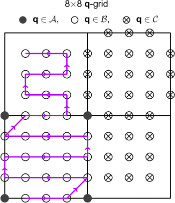
Figure 3: Example of space-filling curve employed to order the phonon wavevectors along a one-dimensional array. For illustration purposes we show the curve passing through the ${\bf q}$-points in set $\mathcal{B}$ of the Brillouin zone grid shown in Fig. 1.

At this point we are left with the determination of the signs $S_{{\bf q}\nu}$. Here we could proceed with a global optimization of all the signs, using Eq. (58). However, in order to keep the algorithm as simple as possible, we proceed with a partial optimization as follows. We order the ${\bf q}$-points along a path that is designed to span the entire set $\mathcal{B}$ in the Brillouin zone. A simple representative path in two dimensions is shown in Fig. 3. More complex choices such as the Peano-Hilbert space-filling curve are possible Sagan (1994), but we have not explored these alternatives. The only requirement for the construction of this path is that it should exhibit ‘locality’, in the sense that pairs of ${\bf q}$-points which are close in the Brillouin zone should also be close along the path, so that Eq. (53) is fulfilled. We then group the ${\bf q}$-points along the path in sets of neighbors, with $2^{n-1}$ ${\bf q}$-points per set. The signs in each set are determined by extracting $2^{n-1}$ sequences from the $2^{n}$ possible combinations, as explained in Sec. V.4, excluding antithetic sets. Then we consider $2^{n-1}$ consecutive sets like $\mathcal{D}$, and we choose the signs as cyclic permutations of those from the first set. This procedure allows us to assign $S_{{\bf q}\nu}$ for a total of $2^{2(n-1)}$ ${\bf q}$-points. At this stage we evaluate the error $E(\{S_{{\bf q}\nu}\})$ of Eq. (58) for these ${\bf q}$-points. If the error is above a pre-defined threshold (defined as an external parameter, say $\delta=5$%) then we restart the procedure by performing a new selection of the $2^{n-1}$ sign sequences and their order in the first $\mathcal{D}$ set.

We emphasize that the above optimization is unnecessary for large supercells, and many other choices of signs will lead to essentially the same results. This procedure is only advantageous when trying to obtain temperature-dependent properties using small supercells (e.g. 4$\times$4$\times$4 supercells). If the set $\mathcal{B}$ contains more than $2^{2(n-1)}$ ${\bf q}$-points, then we continue the sequence by restarting from the beginning. We note that, while this procedure does not necessarily respect the periodic gauge across the Brillouin-zone boundaries, this does not constitute a limitation since we are only interested in minimizing $E(\{S_{{\bf q}\nu}\})$.

Having established the signs $S_{{\bf q}\nu}$, we finally compute the ZG displacement using Eq. (2). In this expression the temperature $T$ is an external parameter and enters via the Bose-Einstein factors $n_{{\bf q}\nu}$.

VI.3 Smooth gauge of phonon eigenmodes along a path in reciprocal space

In order to satisfy Eq. (51), we perform unitary transformations of phonon eigenmodes at adjacent ${\bf q}$-points on the space-filling curve described in Sec. VI.2. The transformation is defined in such a way that similar eigenmodes at different ${\bf q}$-points have a similar complex phase, and the ordering of eigenmodes is preserved in the case of branch crossing. This is equivalent to enforcing a smooth Berry connection across the Brillouin zone Vanderbilt (2018). These ideas are related to standard concepts used in the theory of maximally-localized Wannier functions Marzari and Vanderbilt (1997).

Given two adjacent reciprocal-space vectors ${\bf q}$ and ${\bf q}+\Delta{\bf q}$, we seek for a transformation such that $e_{\kappa{\alpha},\nu}({\bf q})$ and $e_{\kappa{\alpha},\nu}({\bf q}+\Delta{\bf q})$ be as similar as possible. We can define similarity between eigenmodes using the overlap matrix:

$$M_{\nu\nu^{\prime}}=\sum_{\kappa{\alpha}}e_{\kappa{\alpha},\nu}({\bf q}+\Delta{\bf q})e^{*}_{\kappa{\alpha},\nu^{\prime}}({\bf q}).$$ (59)

Using this definition and using the orthonormality relations in Eq. (69) we have:

$$e_{\kappa{\alpha},\nu}({\bf q}+\Delta{\bf q})=\sum_{\nu^{\prime}}M_{\nu\nu^{\prime}}e_{\kappa{\alpha},\nu^{\prime}}({\bf q}).$$ (60)

For the modes $e_{\kappa{\alpha},\nu}({\bf q})$ and $e_{\kappa{\alpha},\nu}({\bf q}+\Delta{\bf q})$ to be as similar as possible, the overlap matrix $M_{\nu\nu^{\prime}}$ needs to be as close as possible to the identity matrix. Generally this is not the case since the diagonalization of the dynamical matrix at different ${\bf q}$-points introduces an arbitrary gauge in the normal modes. To address this problem we perform a transformation of $e_{\kappa{\alpha},\nu}({\bf q}+\Delta{\bf q})$ as follows:

$$e^{\prime}_{\kappa{\alpha},\nu}({\bf q}+\Delta{\bf q})=\sum_{\nu^{\prime}}U_{\nu\nu^{\prime}}e_{\kappa{\alpha},\nu^{\prime}}({\bf q}+\Delta{\bf q}),$$ (61)

where $U_{\nu\nu^{\prime}}$ is a unitary rotation among the vibrational eigenmodes. After this transformation, the new overlap matrix reads:

$$M^{\prime}_{\nu\nu^{\prime}}=\sum_{\kappa{\alpha}}e^{\prime}_{\kappa{\alpha},\nu}({\bf q}+\Delta{\bf q})e^{*}_{\kappa{\alpha},\nu^{\prime}}({\bf q})=\sum_{\mu}U_{\nu\mu}M_{\mu\nu^{\prime}}.$$ (62)

We want to find the unitary matrix $U$ such that $M^{\prime}=UM$ is as close as possible to the identity $I$. To this aim we need to minimize the quantity $||M^{\prime}-I||^{2}$, where $||A||$ represents the Frobenius norm of the matrix $A$ and is given by $||A||^{2}={\rm Tr}(A^{\dagger}A)$. Using $M^{\prime}=UM$ we can write:

$$||M^{\prime}-I||^{2}={\rm Tr}(M^{\dagger}M+I)-{\rm Tr}(M^{\dagger}U^{\dagger}+UM).$$ (63)

Minimizing the left-hand side with respect to $U$ is equivalent to mazimizing ${\rm Tr}(M^{\dagger}U^{\dagger}+UM)$. Using the properties of the matrix trace this is the same as maximizing $\hskip 0.5pt{\rm Re}\,{\rm Tr}\,(UM)$.

The matrix $M$ is not Hermitian in general, but it can be decomposed via SVD as:

$$M=LSR^{\dagger},$$ (64)

where $L$ and $R$ are unitary matrices and $S$ is a diagonal matrix with non-negative real values on the diagonal. With these definitions, it can be shown that the matrix $U$ that maximizes $\hskip 0.5pt{\rm Re}\,{\rm Tr}\,(UM)$ is precisely $U=RL^{\dagger}$ Gander and Hrebicek (1997).

In order to use this strategy in practical calculations, we determine unitary transformations for each ${\bf q}$-point along a space-filling curve, by evaluating overlap matrices $M$ between each pair of successive ${\bf q}$-points, say ${\bf q}_{1}$ and ${\bf q}_{2}$. Then we apply the transformation $U$ to the modes in ${\bf q}_{2}$, and repeat the procedure for ${\bf q}_{2}$ and ${\bf q}_{3}$, and so on for all wavevectors.

Figure 4 shows the eigenmodes $e_{\kappa{\alpha},\nu}({\bf q})$ of silicon before and after the procedure just described. We can see that the resulting eigenmodes vary continuously between adjacent ${\bf q}$-points, as desired.

VI.4 Generation of temperature-dependent band structure by Brillouin-zone unfolding

In this section we present the recipe for calculating spectral functions that represent momentum-resolved density of states of the electrons at a given temperature. In order to obtain the spectral functions in the Brillouin zone of the primitive unit cell we employ the following unfolding procedure.

The spectral function is defined as Popescu and Zunger (2012); Medeiros et al. (2014):

$$A_{\bf k}(\varepsilon;T)=\sum_{m{\bf K}}P_{m{\bf K},{\bf k}}(T)\,\delta[\varepsilon-\varepsilon_{m{\bf K}}(T)],$$ (65)

where $P_{m{\bf K},{\bf k}}(T)$ are temperature-dependent spectral weights given by:

$$P_{m{\bf K},{\bf k}}(T)=\sum_{n}|\langle\psi^{\rm SC}_{m{\bf K}}(T)|\psi^{\rm PC}_{n{\bf k}}\rangle|^{2}.$$ (66)

In these expressions $\varepsilon_{m{\bf K}}(T)$ and $\psi^{\rm SC}_{m{\bf K}}(T)$ represent eigenvalue and wavefunction of a Kohn-Sham state in the supercell, respectively, obtained from a calculation with the ZG displacement at the temperature $T$; $\psi^{\rm PC}_{n{\bf k}}$ denotes a state in the primitive unit cell. We employ lower (upper) case bold fonts to indicate wavevectors in the primitive cell (supercell). The integral is over a volume that encompasses the supercell and is commensurate both with ${\bf K}$ and ${\bf k}$. The equivalence between Eq. (65) and the standard definition of the electron spectral function using the Lehmann representation is demonstrated in Ref. [Allen et al., 2013].

We now expand Kohn-Sham states in a planewaves basis set as follows: $\psi^{\rm PC}_{n{\bf k}}({\bf r})=V^{-1/2}\sum_{\bf g}c^{\rm PC}_{n{\bf k}}({\bf g})\exp[i({\bf k}+{\bf g})\cdot{\bf r}]$, $\psi^{\rm SC}_{n{\bf K}}({\bf r};T)=V^{-1/2}\sum_{\bf G}c^{\rm SC}_{n{\bf K}}({\bf G};T)\exp[i({\bf K}+{\bf G})\cdot{\bf r}]$, where $V$ is the volume where the wavefunctions are normalized. By replacing these expansions inside Eq. (66) and using the resolution of identity $\sum_{n}c^{\rm PC}_{n{\bf k}}({\bf g})c^{\rm PC,*}_{n{\bf k}}({\bf g}^{\prime})=\delta_{{\bf g}{\bf g}^{\prime}}$ one obtains:

$$P_{m{\bf K},{\bf k}}(T)=\sum_{\bf g}|c^{{\rm SC}}_{m{\bf K}}({\bf g}+{\bf k}-{\bf K};T)|^{2}.$$ (67)

We note that in the last expression only the planewaves coefficients of the supercell state appear; therefore the calculation of the spectral function at finite temperature does not require explicit projections onto the states of the primitive cell. In actual calculations we select a ${\bf k}$-path in the Brillouin zone of the primitive cell, and for each ${\bf k}$-point we proceed as follows: we identify all the supercell ${\bf K}$-points that unfold into ${\bf k}$ via a reciprocal lattice vector ${\bf G}$ of the supercell; for each of these points we evaluate the weights $P_{m{\bf K},{\bf k}}(T)$ using Eq. (67); then we use the calculated weights inside Eq. (65). In the case of ultrasoft pseudopotentials, which we employed for calculations on monolayer MoS₂ in Sec. VII.4, we use a slightly modified version of Eq. (67) to account for the augmentation charge Vanderbilt (1990). Starting from the spectral function $A_{\bf k}(\varepsilon;T)$, we extract the renormalized band structure by numerically identifying the quasiparticle peaks along the energy axis.

In principle one could also evaluate a momentum- and band- resolved spectral function, by considering scalar products like in Eq. (66) but without the summation over the states $n$ of the primitive unit cell. In this case Eq. (67) must be replaced by a more complicated expression which requires an explicit evaluation of wavefunctions in the primitive unit cell. We explored this possibility, but we found that in order to achieve numerical convergence one would need an impractically large number of bands in the supercell.

VII Summary of procedure and numerical results

In this section we summarize the procedure for the calculation of temperature-dependent band structures using the ZG displacement, and we discuss our results for silicon, gallium arsenide, and monolayer molybdenum disulfide. The special displacement method consists of the following steps:

• We compute the vibrational eigenmodes $e_{\kappa{\alpha},\nu}({\bf q})$ and eigenfrequencies $\omega_{{\bf q}\nu}$ in the unit cell using DFPT on a coarse uniform grid of ${{\bf q}}$-points.

• In preparation for calculations on a supercell of size $N_{1}\!\times\!N_{2}\!\times N_{3}$, we interpolate the vibrational eigenmodes and frequencies on a finer ${{\bf q}}$-points grid with the same size as the supercell, $N_{1}\!\times\!N_{2}\!\times N_{3}$. We partition this grid into the sets $\mathcal{A}$, $\mathcal{B}$, and $\mathcal{C}$.

• We enforce a smooth Berry connection for the vibrational eigenmodes. To this aim we perform unitary transformations that makes eigenmodes at nearby ${\bf q}$-points as similar as possible, as described in Sec. VI.3.

• We build an $N_{1}\!\times\!N_{2}\!\times N_{3}$ supercell with the atoms displaced by $\Delta{\bm{\tau}}_{p\kappa}$ given in Eq. (2). The signs $S_{{\bf q}\nu}$ in Eq. (2) are determined using the procedure described in Sec. V.4.

• To compute band structures, we first set up the ${\bf k}$-point path in the Brillouin zone of the primitive cell, then we obtain the folded ${\bf k}$-points in the Brillouin zone of the supercell. We perform a DFT band structure calculation in the supercell, and we unfold the result using the method of Ref. [Popescu and Zunger, 2012]. This procedure is discussed in Sec. VI.

In this manuscript we focus on temperature-dependent band structures to limit the length of the presentation. For calculations of temperature-dependent optical spectra, photoelectron spectra, tunneling spectra, or transport coefficients, steps (i)-(iv) above remain the same, while step (v) shall be replaced by the calculation of the required property.

We emphasize that the ZG displacement in Eq. (2) does not contain eigenmodes with ${\bf q}\in\mathcal{A}$. These eigenmodes correspond to stationary lattice waves, and break the crystal symmetry. In the following sections we show how this observation can be used to analyze the convergence and the accuracy of the calculations as a function of supercell size.

The main difference between Eq. (2) and the displacement provided in our previous work [Eq. (5) of Ref. [Zacharias and Giustino, 2016]] is that here a more structured choice of signs allow us to better control the convergence rate and to perform accurate calculations using relatively small supercells.

VII.1 Thermal mean-square displacements of Si, GaAs, and MoS₂

In Fig. 5(a) we compare the probability distribution $P(\Delta\tau_{p\kappa{\alpha}};T)$ in Eq. (16) evaluated for silicon at $T=0$ K with an histogram of the displacements obtained from the ZG formula in Eq. (2). The histogram is obtained numerically by binning the values of $\Delta\tau_{p\kappa{\alpha}}$ for all atoms along the [100] direction. It is remarkable that the distribution provided by the ZG displacement follows the exact thermodynamic average with very high precision. The choice of the Cartesian direction is not important in this case, since silicon is isotropic. In fact the inset of Fig. 5(a) shows that the distribution in the (100) plane is also isotropic. For completeness we also show in Fig. 5(b) how the ZG displacement appears in a three-dimensional rendering.

In Fig. 6(a)-(c) we show the thermal mean-square displacements of Si, GaAs, and MoS₂ calculated using the ZG displacements (colored disks), the mean-square displacements evaluated using the exact expression in Eq. (17) (grey disks), and experimental data from XRD where available (triangles) Aldred et al. (1973); Stern et al. (1980); Matsushita and Kohra (1974); Schönfeld et al. (1983). We can see that the ZG displacement yields mean-square displacements in excellent agreement with Eq. (17), and that the agreement between our calculations and experiments is also very good. These successful comparisons reinforce the notion that the ZG displacement provides a very accurate classical representation of a thermodynamic average over the quantum fluctuations of the atomic positions.

The ZG displacement can also be employed to obtain the thermal displacement ellipsoids and compare the complete ADP tensor $U_{\kappa,{\alpha}{\beta}}(T)$ of Eq. (18) with experiments. In Fig. 6(d)-(f) we show the computed thermal ellipsoids of Si, GaAs, and MoS₂ at $T=300$ K. The ellipsoids of Si, Ga, and As are found to be spheres with radius 0.49 Å², 0.59 Å², and 0.50 Å², respectively. These findings are consistent with the cubic symmetry of the Si and GaAs lattices. In the case of MoS₂, the ellipsoids reflect the two-dimensional nature of the material: the in-plane parameters $U_{\parallel}$ are 0.22 Å² and 0.42 Å² for Mo and S atoms, respectively; the out-of-plane parameters $U_{\perp}$ are 0.82 Å² and 0.86 Å² for Mo ans S, respectively. In all cases the ADPs obtained from the ZG displacements are within 25% of the corresponding experimental values Aldred et al. (1973); Stern et al. (1980); Matsushita and Kohra (1974); Schönfeld et al. (1983).

VII.2 Temperature dependent band structure of Si

Figure 7 shows our results and analysis for the band structure of Si at finite temperature. Full computational details, including the evaluation of the spectral function and band energies in the primitive unit cell, are provided in Sec. VI; here we only mention that the calculations are based on DFT in the local density approximation (LDA). In Fig. 7(a), we show the spectral function $A_{{\bf k}}(\varepsilon;T)$ obtained from the ZG displacement in a 8$\times$8$\times$8 supercell. We consider $T=0$ K to focus on the effect of zero-point renormalization. The spectral function provides the momentum-resolved electronic density of states Abrikosov et al. (1963), and it is shown as a colormap. In Fig. 7(b) we compare the bands $\varepsilon_{n{\bf k}}(T)$ extracted from the spectral function $A_{\bf k}(\varepsilon;T)$ with the usual DFT band structure evaluated at clamped ions; in particular we consider the dispersions along the L$\Gamma$X path of the Brillouin zone for $T=0$ K (blue) and $T=300$ K (green); the DFT bands at clamped ions are in black. This calculation indicates that, as a result of zero-point motion, the energy of the valence band maximum (VBM) at $\Gamma$ increases by 35 meV, while the energy of the indirect conduction band minimum (CBM) at $\simeq 0.87\,\Gamma X$ decreases by 22 meV. These values are in excellent agreement with Ref. [Poncé et al., 2015], which obtained 35 meV and 21 meV, respectively, when using the perturbative Allen-Heine approach and the adiabatic approximation.

From the band structure in Fig. 7(b) we can also extract the phonon-induced mass-enhancement. For simplicity we focus on the longitudinal electron mass of silicon, and we define the coupling strength $\lambda_{T}$ such that $m^{*}_{l}(T)=(1+\lambda_{T})m^{*}_{l}$ where $m_{l}^{*}={0.95}\,m_{e}$ is the DFT mass at clamped ions. From the calculated bands we obtain $\lambda_{T}=0.03$ and $0.04$ for $T=0$ K and $T=300$ K, respectively. This finding is in agreement with the mass renormalization reported in Ref. [Poncé et al., 2018].

Our calculated band gap narrowing due to zero-point effects is 57 meV. This value is in very good agreement with previous calculations based on non-perturbative adiabatic approaches, yielding 56-65 meV Monserrat and Needs (2014); Monserrat (2016a); Zacharias et al. (2015); Zacharias and Giustino (2016); Karsai et al. (2018a) as well as with experimental values, in the range of 62-64 meV Cardona (2001, 2005). Ref. [Poncé et al., 2015] showed that non-adiabatic corrections within the Allen-Heine theory increase the zero-point renormalization by 8 meV Poncé et al. (2015). This effect is not captured by the present special displacement method, which is in essence an adiabatic approach. We also point out that the most recent GW calculations using an earlier version of the present approach Karsai et al. (2018a) yield a slightly larger gap renormalization of 66 meV. This is expected given that the electron-phonon interaction is overscreened in DFT/LDA due to the band gap problem.

In order to analyze the convergence behavior of the SDM, in Fig. 7(c) we plot the dependence of the zero-point band gap renormalization on the supercell size. Two sets of data are shown. The green lines and datapoints correspond to calculations performed using Eq. (2). The black lines and grey datapoints were obtained after modifying Eq. (2) to include the contributions of phonons with ${\bf q}\in\mathcal{A}$. Phonons with ${\bf q}\in\mathcal{A}$ correspond to stationary waves in the primitive unit cell (e.g. ${\bf q}=0$ phonons). As we demonstrate in Sec. V.4, in the thermodynamic limit of infinite supercell the contribution of these modes vanishes identically. Therefore, the calculations performed by including or excluding phonons with ${\bf q}\in\mathcal{A}$ in the ZG displacement given by Eq. (2) converge to the same limit. However, by considering only ${\bf q}\in\mathcal{B}$ phonons as in Eq. (2) we reach convergence from the bottom (in terms of magnitude); while by including phonons with ${\bf q}\in\mathcal{B}$ and ${\bf q}\in\mathcal{A}$ we reach convergence from the top. By construction the converged answer must lie in between these two limits, therefore the analysis presented in Fig. 7(c) can be used as a way to quantify the convergence error of the calculations. For example the data obtained for a 10$\times$10$\times$10 supercell in Fig. 7(c) show that the fully converged result for an infinitely-large supercell will be in the interval 55-65 meV. This observation carries general validity for all the systems considered in this work.

The inset of Fig. 7(c) shows the spectral function near the threefold degenerate VBM of silicon, as computed using the ZG displacement for a 4$\times$4$\times$4 supercell at $T=0$ K. If we include ${\bf q}\in\mathcal{A}$ points in the ZG displacement, then the crystal symmetry is broken, and by consequence we observe a band splitting (black line). In contrast, when we use the pure ZG displacement from Eq. (2), i.e. without phonons with ${\bf q}\in\mathcal{A}$, the band degeneracy is correctly preserved. This analysis indicates that, when performing electron-phonon calculations using non-perturbative supercell approaches, ${\bf q}=0$ phonons as well as all phonons with ${\bf q}\in\mathcal{A}$ are the least representative since they break crystal symmetry, which may lead to calculation artifacts. This issue is resolved by the present formulation of the ZG displacement as provided by Eq. (2).

In Fig. 7(d) we compare our calculations of the indirect band gap of silicon using the SDM with experiments Alex et al. (1996), up to $T=500$ K. To facilitate comparison we scissor-shifted our DFT/LDA results by 0.73 eV, which is close to the GW correction reported in Ref. [Lambert and Giustino, 2013]. The agreement between our calculation and experiment is very good, except that we underestimate slightly the temperature slope. This effect is a well-known consequence of the fact that the strength of the electron-phonon interaction is underestimated by DFT/LDA; the slope can be improved by using GW calculations in combination with the SDM, as demonstrated in Ref. [Karsai et al., 2018a].

VII.3 Temperature dependent band structure of GaAs

Figure 8 shows our calculated band structure of GaAs at finite temperature. Also in this case we employ DFT and the LDA, as described in Sec. VI. In Fig. 8(a) we have the spectral function $A_{{\bf k}}(\varepsilon;T)$ at $T=0$ K as a color map, and in Fig. 8(b) we have the bands extracted from the spectral function at $T=0$ K (blue) and $T=300$ K (green). The bands at clamped ions are shown in black for comparison. For simplicity we are not including spin-orbit coupling in the calculations, therefore we do not see the spin-orbit splitting of the split-off holes in the valence bands Chelikowsky and Cohen (1976); Jancu et al. (1998); Richard et al. (2004). Since the holes at the top of the valence band have the same orbital character, we expect a similar zero-point renormalization for the split-off holes.

From the data in Fig. 8(b) we obtain zero-point corrections to the valence and conduction band edges at $\Gamma$ of $+21$ meV and $-11$ meV, respectively. The resulting band gap narrowing, $\Delta E_{\rm g}=32$ meV, lies within the experimental range of $57\pm 29$ meV Lautenschlager et al. (1987). The calculations in Fig. 8(b) are performed using an 8$\times$8$\times$8 supercell. To better compare with the finite-differences results of Ref. [Antonius et al., 2014], we repeated the calculations with a smaller, 4$\times$4$\times$4 supercell. In this case we obtain $\Delta E_{\rm g}=25$ meV, which matches the value of 25 meV reported in Ref. [Antonius et al., 2014]. It is well established that GW quasiparticle corrections change these results by strengthening the electron-phonon coupling Antonius et al. (2014); Karsai et al. (2018a): in order to incorporate this effect it will be sufficient to perform a GW calculation using the ZG displacement.

From the band structure in Fig. 8(b) we can determine the phonon-induced mass-enhancement. Since we are not including spin-orbit effects, we only report the value for the CBM at $\Gamma$. By denoting $m_{e}^{*}=0.056\,m_{e}$ the conduction band mass at clamped ions, we find $m^{*}_{e}(T)=(1+\lambda_{T})m^{*}_{e}$ with $\lambda_{T}=0.005$ and $0.007$ for $T=0$ K and $T=300$ K, respectively. We are unaware of previous calculations of the mass renormalization in GaAs as a function of temperature.

In Fig. 8(c) we show the convergence of the zero-point renormalization of the direct gap of GaAs with respect to the supercell size. The converged value obtained with Eq. (2) is $\Delta E_{\rm g}=32$ meV and is obtained using an 8$\times$8$\times$8 supercell. As for the case of Si in Fig. 7(c), also for GaAs the threefold degeneracy of the VBT is preserved when using the ZG displacement. And also in this case, if we include phonons with ${\bf q}\in\mathcal{A}$ in Eq. (2), the degeneracy is lifted due to symmetry breaking, as it can be seen in the inset of Fig. 8(c).

In previous work it has been suggested that in the case of polar materials it might be impossible to achieve convergence within the adiabatic approximation Poncé et al. (2015). Here we wish to emphasize that the divergence of perturbative approaches for polar materials is not a consequence of the adiabatic approximation, but it results from taking the limit $\omega_{{\bf q}\nu}\rightarrow 0$ before performing the integration over phonon wavevectors to obtain the Fan-Migdal self-energy Giustino (2017). When the limit $\omega_{{\bf q}\nu}\rightarrow 0$ is correctly performed after evaluating the integral over ${\bf q}$, there is no divergence. The correct procedure can be found in Sec. IV of the early work by Fan Fan (1951) and is summarized in Appendix C. Figure 8(c) shows indeed that adiabatic calculations using the SDM converge smoothly as a function of supercell size, and that the fully converged band gap renormalization lies in a very narrow bracket between 32 meV (ZG displacement without ${\bf q}\in\mathcal{A}$ phonons) and 36 meV (ZG displacement with ${\bf q}\in\mathcal{A}$ phonons) already for a 8$\times$8$\times$8 supercell.

Generally speaking, the smooth and fast convergence of the SDM can be ascribed to the fact that the formalism relies on a standard DFT calculation for a supercell with displaced atoms. This calculation is intrinsically easier to converge than perturbative approaches. In fact perturbative methods require stringent ${\bf q}$-point sampling to evaluate principal-value integrals of first-order poles that appear in the Fan-Migdal and Debye-Waller self-energies; furthermore these integrals yield large and opposite contributions, so the final result is obtained by subtracting two large numbers. The SDM method circumvents these numerical challenges.

In Fig. 8(d) we show our results for the direct gap of GaAs using the ZG displacement, in the temperature range 0-500 K, and we compare with experimental data from Ref. [Lautenschlager et al., 1987]. In order to take into account the non-negligible expansion of the GaAs lattice with temperature, we employ the quasi-harmonic approximation. We use a scissor-shift of 0.53 eV to mimic GW corrections as reported in Ref. [Remediakis and Kaxiras, 1999]. The slight underestimation of the experimental slope with temperature can be corrected by performing GW calculations instead of standard DFT/LDA Antonius et al. (2014); Karsai et al. (2018a), but overall the agreement between the present calculations and experiments is very good.

For completeness, we also mention that the results shown in Fig. 8(d) and obtained from the analysis of temperature-dependent band structures are in excellent agreement with the values that we obtained in an earlier work by analyzing the joint density of states Zacharias and Giustino (2016).

VII.4 Temperature dependent band structure of monolayer MoS₂

Figure 9 shows our calculated temperature-dependent band structure of monolayer MoS₂, as an example of application of the SDM to two-dimensional materials. In this case we employed the PBE exchange and correlation functional Perdew et al. (1996), and fully relativistic ultrasoft pseudopotentials Vanderbilt (1990) to take spin-orbit coupling into account (Sec. VI).

In Fig. 9(a) we have the spectral function of MoS₂ at $T=0$ K obtained from the ZG displacement in a 10$\times$10$\times$1 supercell. By extracting the corresponding temperature-dependent bands we obtain a spin-orbit splitting of 136 meV for the valence band states at $K$, to be compared to the clamped-ion value of 142 meV. Our calculation is in agreement with the spliting of 135 meV obtained in Ref. [Molina-Sánchez et al., 2016] within the Allen-Heine theory. We also determined the electron effective mass renormalization at the $K$ point, and found $\lambda_{T}\simeq 0.04$ and $\simeq 0.06$ for $T=0$ K and $T=300$ K, respectively. These latter two values are not fully converged since we used finite differences with a coarse ${\bf k}$-point spacing of $6\cdot 10^{-3}\,2\pi/a$.

In Fig. 9(b) and (c) we show convergence tests for the gap renormalization. In Fig. 9(b) we have the renormalization as a function of interlayer separation by keeping the in-plane supercell size fixed; in (c) we vary the supercell size, keeping the interlayer separation constant. As in the case of the three-dimensional materials Si and GaAs, the band gap narrowing converges relatively quickly with the size of the cell; furthermore the calculations are not very sensitive to the size of the vacuum region provided periodic replica are separated by more than 10 Å.

For a 10$\times$10$\times$1 supercell we obtain a zero-point gap renormalization of 64 meV using the ZG displacement. By including also ${\bf q}\in\mathcal{A}$ phonons in Eq. (2) the value changes only slightly to 65 meV, therefore we estimate an error with respect to the fully converged result of less than 1 meV. Our result is in good agreement with the perturbative calculations of Ref. [Molina-Sánchez et al., 2016], which reported 75 meV. The residual difference may be due to the ‘rigid-ion’ approximation used in the Allen-Heine approach of Ref. [Molina-Sánchez et al., 2016], and to differences in the DFT exchange and correlation functionals employed.

In Fig. 9(d) we compare our calculated temperature-dependent band gap of MoS₂ (green) with experimental data from Ref. [Park et al., 2018] (black). To facilitate comparison we introduced a scissor correction of 0.34 eV to match the measured band gap at 4 K. This correction is similar to that obtained using GW and the Bethe-Salpeter equation (BSE) Shi et al. (2013). Unlike in Si and GaAs, here the calculated data follow the experimental trend very closely. This is unexpected since we are computing electron-phonon effects at the DFT/PBE level, and suggests that quasiparticle corrections of the electron-phonon coupling Zhenglu et al. (2019) are not significant in MoS₂.

VII.5 General remarks on the SDM results

The applications to Si, GaAs, and MoS₂ described in the previous sections show that the SDM yields temperature-dependent bands of the same quality as perturbative approaches based on the Allen-Heine theory. In particular, the capability to access momentum-resolved quantities such as temperature-renormalization at specific ${\bf k}$-points and the phonon-induced enhancement of the band mass are entirely novel, and considerably expand the range of applicability of the ZG displacement.

One important point of note is that the present reciprocal-space formulation of the ZG displacement allowed us to identify and remove the contributions of vibrational modes that break crystal symmetry. This improvement is important in order to avoid spurious and uncontrolled lifting of electronic degeneracy. Since the symmetry-breaking modes are those with wavevector ${\bf q}\in\mathcal{A}$, that is phonons corresponding to standing Bloch waves, the present analysis and results demonstrate that these modes (especially ${\bf q}=0$ phonons) are the least representative in a thermodynamic average, and should be avoided for accurate calculations.

Another interesting point is that we can bracket the fully converged results by performing two calculations: one with the pure ZG displacement of Eq. (2), and one with the modified version including ${\bf q}\in\mathcal{A}$ phonons. This provides a simple and effective strategy to quantify the convergence error as a function of supercell size.

We also found that, when used in conjunction with the ZG displacement, the adiabatic approximation does not suffer from the convergence problems that are encountered in perturbative approaches for polar materials. This advantage arises from the fact that the special displacement method does not require integrating over poles as in perturbative approaches, and the calculation is as easy as a standard calculation at clamped ions.

For the systems considered in this work, the supercells required to achieve relatively accurate results are surprisingly small. For example, the ZG displacement in a 4$\times$4$\times$4 Si supercell (128 atoms) yields a zero-point renormalization which differs by less than 10% from the fully converged value; for GaAs we need a 6$\times$6$\times$6 supercell (432 atoms) to achieve similar accuracy; for MoS₂ a 6$\times$6$\times$1 supercell (72 atoms) is enough to converge the results within 10%. This indicates that the ZG displacement can be used to perform calculations with relatively small supercells, and this may open the way to post-DFT calculations at finite temperature, including GW quasiparticle calculations and exciton calculations via the BSE method.

VIII Conclusions and outlook

In this manuscript we develop a new methodology for performing electronic structure calculations at finite temperature. In a nutshell, this method consists of performing a single calculation in a supercell where the atoms have been displaced according to Eq. (2). We refer to this displacement as the ZG displacement, and to the methodology as the special displacement method.

This work follows our earlier study in Ref. [Zacharias and Giustino, 2016], where the original idea was first proposed. The key novelty of the present study is that we reformulate the entire theory using a compact and rigorous reciprocal space formulation, building on density functional perturbation theory. This new formulation allows us to go beyond angle-integrated electronic and optical spectra, and to compute complete band structures at finite temperature. We demonstrate this concept for three-dimensional bulk semiconductors, silicon and gallium arsenide, and for a two-dimensional semiconductor, monolayer molybdenum disulfide. In all cases our results match the accuracy of established perturbative techniques based on the Allen-Heine theory. The added advantage of the present approach over perturbative methods is that it does not require the evaluation of self-energy energy poles, and it does not require the rigid-ion approximation for the Debye-Waller self-energy. As a consequence, the method is robust, reliable, and simple to use.

Beyond demonstrating calculations of band structures at finite temperature, we show that the ZG displacement accurately reproduces the characteristic anisotropic displacement parameters measured by X-ray crystallography, and can be used to determine thermal ellipsoids as a function of temperature. Therefore the ZG displacement represents an accurate classical snapshot of thermal disorder in solids, and eliminates the need for the stochastic sampling of the nuclear wavefunctions.

More fundamentally, we show that the ZG displacement can be understood as the best single-point approximant to a thermodynamic Feynman path-integral. This link may open new avenues in the study of path integrals using the quantum-classical analogy and special displacements.

In the present approach, the choice of the atomic displacements is carefully performed by first establishing a smooth Berry connection among vibrational eigenmodes in the Brillouin zone, and then by choosing the phase of each eigenmode using rigorous sum rules. This approach allows us to prove that the ZG displacement yields the exact Williams-Lax average of an electronic observable in the thermodynamic limit of infinite supercell. We also provide procedures for accelerating the convergence of the calculations for those cases where only small supercells are within reach.

For reasons of space we only discussed applications to finite-temperature band structures, but we emphasize that this methodology is much more general. For example the earlier version of this method Zacharias and Giustino (2016) has already been applied to compute phonon-assisted optical properties, dielectric functions, GW quasiparticle corrections, zero-point renormalization of band gaps, exciton-phonon couplings, and charge transport. This broad range of applications is possible because the Williams-Lax theory can be employed to compute any property which can be expressed as a Fermi’s golden rule.

The present extension of the special displacement method to compute entire band structures is particularly appealing for testing quasiparticle corrections at finite temperature. Since only one supercell calculation is required, and since we developed a new algorithm to accelerate convergence with respect to the supercell size, this approach opens the way to systematic many-body calculations of band structures at finite temperature.

Up to this point the SDM relied on the harmonic approximation. It would be interesting to consider extensions to anharmonic systems. We expect that the method will work seamlessly in conjunction with the quasi-harmonic approximation Fleszar and Gonze (1990); Baroni et al. (2010) and with the self-consistent harmonic approximation Hellman et al. (2011); Errea et al. (2014). In fact, in both cases the original anharmonic potential is replaced by its ‘best’ harmonic approximation; after this replacement the SDM method can be used without changes. In the case of strongly anharmonic systems, for example in the presence of double-well potential energy surfaces, it should be possible to modify the present method by treating all the harmonic modes as described in this manuscript, and by adapting the ZG configuration to describe averages over double-well quantum nuclear wavefunctions. The feasibility and accuracy of this approach will have to be demonstrated in future work.

Appendix A Dynamical matrix and Born-von Kármán boundary conditions

Here we summarize the relations between normal modes $e_{\kappa{\alpha},\nu}({\bf q})$ obtained from the diagonalization of the dynamical matrix at each ${\bf q}$ wavevector, and the standard sum rules resulting from the Born-von Kármán boundary conditions.

In the harmonic approximation the dynamical matrix $D_{\kappa{\alpha},\kappa^{\prime}{\alpha}^{\prime}}({\bf q})$ at each ${\bf q}$-point and the vibrational eigenmodes and frequencies satisfy the equation: Giustino (2017)

$$\sum_{\kappa^{\prime}{\alpha}^{\prime}}D_{\kappa{\alpha},\kappa^{\prime}{\alpha}^{\prime}}({\bf q})e_{\kappa^{\prime}{\alpha}^{\prime},\nu^{\prime}}({\bf q})=\omega_{{\bf q}\nu}e_{\kappa{\alpha},\nu}({\bf q}).$$ (68)

Since the dynamical matrix is Hermitian, the eigenmodes form an orthonormal basis:

$$\sum_{\nu}e_{\kappa{\alpha},\nu}({\bf q})e^{*}_{\kappa^{\prime}{\alpha}^{\prime},\nu}({\bf q}) = \delta_{\kappa\kappa^{\prime}}\delta_{{\alpha}{\alpha}^{\prime}},$$ (69)

$$\sum_{\kappa{\alpha}}e^{*}_{\kappa{\alpha},\nu}({\bf q})e_{\kappa{\alpha},\nu^{\prime}}({\bf q}) = \delta_{\nu\nu^{\prime}}.$$ (70)

Equation (68) implies the relations: Giustino (2017)

$$e_{\kappa{\alpha},\nu}(-{\bf q})=e^{*}_{\kappa{\alpha},\nu}({\bf q}),\,\,\,\,\,\,\,\,\,\omega_{{\bf q}\nu}=\omega_{-{\bf q}\nu},$$ (71)

where we followed the convention of Ref. [Maradudin and Vosko, 1968].

We denote the lattice vector pointing to the $p$-th unit cell as ${\bf R}_{p}=n_{p_{1}}{\bf a}_{1}+n_{p_{2}}{\bf a}_{2}+n_{p_{3}}{\bf a}_{3}$, where the ${\bf a}_{i}$ represent the primitive lattice vectors and $n_{p_{i}}$ are integers between 0 and $N_{i}-1$. The Born-von Kármán supercell contains $N_{p}=N_{1}\times N_{2}\times N_{3}$ unit cells. For the uniform grid of phonon wavevectors ${\bf q}$ in the Brillouin zone we choose ${\bf q}=(m_{1}/N_{1}){\bf b}_{1}+(m_{2}/N_{2}){\bf b}_{2}+(m_{3}/N_{3}){\bf b}_{3}$, where the ${\bf b}_{i}$ represent the primitive reciprocal lattice vectors, and $m_{i}$ are integers between 0 and $N_{i}-1$. The vectors ${\bf b}_{i}$ are such that ${\bf a}_{i}\cdot{\bf b}_{j}=2\pi\delta_{ij}$. With these conventions we have the sum rules:

$$\sum_{\bf q}e^{i({\bf R}_{p}-{\bf R}_{p^{\prime}})\cdot{\bf q}} = N_{p}\delta_{pp^{\prime}}$$ (72)

$$\sum_{p}e^{i({\bf q}-{\bf q}^{\prime})\cdot{\bf R}_{p}} = N_{p}\delta_{{\bf q}{\bf q}^{\prime}}.$$ (73)

Appendix B Link between Williams-Lax theory and Feynman’s path integrals

In this appendix we provide some of the mathematical background required to link the Williams-Lax theory with thermodynamic path integrals. The following equations are used in Sec. IV.

Starting from Eq. (20), using the Trotter decomposition $\exp(-\hat{H}_{\rm n}/k_{\rm B}T)=[\exp(-\hat{H}_{\rm n}/Nk_{\rm B}T)]^{N}=\prod_{i=1,N}\exp(-\hat{H}_{\rm n}/Nk_{\rm B}T)$,Ceperley (1995) and inserting the resolutions of identity $\int d\tau_{i}|\tau_{i}\rangle\langle\tau_{i}|=1$ with $i=1,\cdots,N\!-\!1$ in between each product, Eq. (20) becomes:

$$\Gamma_{{\alpha}\rightarrow\beta}(\omega;T) = \frac{1}{Z}\int d\tau_{0}\cdots d\tau_{N-1}$$ (74)

$$\times \!\!\prod_{i=0}^{N-1}\langle\tau_{i}|e^{-\hat{H}_{\rm n}/Nk_{\rm B}T}|\tau_{i+1}\rangle\Gamma_{{\alpha}\rightarrow\beta}^{\{\tau\}}(\omega),\,\,$$

where we introduced $|\tau_{0}\rangle=|\tau_{N}\rangle=|\tau\rangle$ to make the notation more compact.

The nuclear Hamiltonian can be expressed as a sum of kinetic ($\hat{T}$) and potential ($\hat{U}_{\alpha}$) energies, and the exponential in Eq. (74) is rewritten for large $N$ using the Baker-Campbell-Hausdorff formula Kleinert (2009):

$$\lim_{N\rightarrow\infty}e^{-\hat{H}_{\rm n}/Nk_{\rm B}T}=e^{-\hat{T}/Nk_{\rm B}T}e^{-\hat{U}_{\alpha}/Nk_{\rm B}T}.$$ (75)

In this limit the matrix elements appearing in Eq. (74) take the form:

$$\langle\tau_{i}|e^{-\hat{T}\Delta t/\hbar}|\tau_{i+1}\rangle\,e^{-U_{\alpha}(\{\tau_{i+1}\})\Delta t/\hbar},$$ (76)

having defined $\Delta t=\hbar/Nk_{\rm B}T$. The matrix element with the kinetic energy is simplified by inserting the resolution of identity for the eigenstates of the nuclear momentum operators, $\int dk|k\rangle\langle k|=1$, where $\{k\}$ represent a complete set of planewaves associated with the atomic positions $\{\tau\}$. After evaluating terms like $\langle k|\tau_{i}\rangle$ and solving the resulting Gaussian integral, this procedure leads to:

$$\langle\tau_{i}|e^{-\hat{T}\Delta t/\hbar}|\tau_{i+1}\rangle\!=c\prod_{p\kappa{\alpha}}\!e^{-[M_{\kappa}(\tau_{p\kappa{\alpha},i+1}-\tau_{p\kappa{\alpha},i})^{2}/2\Delta t^{2}]\Delta t/\hbar},$$ (77)

where $c$ is a normalization prefactor. By taking the limit of large $N$, which is equivalent to taking $\Delta t\rightarrow 0$, the terms $(\tau_{p\kappa{\alpha},i+1}-\tau_{p\kappa{\alpha},i})/\Delta t$ become the classical velocities of the nuclei, and the exponent of Eq. (77) yields the classical kinetic energy of the nuclei.

The combination of Eqs. (74)-(77) with Eq. (20) yields the link of the Wiliams-Lax transition rate to a thermodynamic Feynman path integral, as shown in Eq. (IV).

Appendix C Adiabatic approximation for polar materials

In recent work it has been proposed that the adiabatic approximation leads to an ill-defined expression Poncé et al. (2015) when computing the band structures of polar semiconductors at finite temperatures.

In this Appendix we show that the divergence noted in Ref. [Poncé et al., 2015] is not related to the adiabatic approximation, but to the procedure employed for evaluating the principal-value integrals appearing in the self-energy.

For simplicity we write the Fan-Migdal self-energy used in Ref. [Poncé et al., 2015] within the Frölich approximation. In particular we consider an electron in an otherwise empty conduction band on mass $m^{*}$, interacting with a single, dispersionless polar longitudinal-optical phonon of frequency $\omega_{\rm LO}$. At zero temperature the self-energy reads Giustino (2017):

$$\Sigma^{\rm FM}_{{\bf k}}(\omega)=\!\int\!\!\frac{d{\bf q}}{\Omega_{\rm BZ}}\frac{|g({\bf q})|^{2}}{\hbar\omega\!-\!\varepsilon_{{\bf k}+{\bf q}}-\hbar\omega_{\rm LO}+i\hbar\eta}.$$ (78)

Here $\varepsilon_{{\bf k}}=\hbar^{2}|{\bf k}|^{2}/2m^{*}$, $\eta$ is a positive infinitesimal, $\Omega_{\rm BZ}$ is the volume of the Brillouin zone, and the Frölich electron-phonon matrix element is given by Sio et al. (2019):

$$|g({\bf q})|^{2}=\frac{e^{2}}{4\pi\epsilon_{0}}\frac{4\pi}{\Omega}\frac{\hbar\omega_{\text{LO}}}{2}\frac{1}{\kappa\,|{\bf q}|^{2}},$$ (79)

where $\Omega$ is the volume of the unit cell. The quantity $\kappa$ is defined as $1/\kappa=1/\epsilon_{0}-1/\epsilon_{\infty}$, with $\epsilon_{0}$ and $\epsilon_{\infty}$ being the static and the high-frequency dielectric constants, respectively.

After replacing Eq. (79) inside (78) and carrying out the algebra we reach the standard expression for the self-energy at the band bottom (${\bf k}=0$, $\omega=0$, $\eta\rightarrow 0$):

$$\Sigma^{\rm FM}=-\alpha\hbar\omega_{\rm LO}\,\frac{q_{\rm LO}}{\pi}\int_{-\infty}^{\infty}\frac{dq}{q^{2}+q_{\rm LO}^{2}},$$ (80)

having defined $q_{\rm LO}^{2}=2m^{*}\hbar\omega_{\rm LO}/\hbar^{2}$. The integration was extended to the infinite crystal since this does not alter the result Fan (1951), and we used the definition of the Fröhlich coupling constant Sio et al. (2019):

$$\alpha=\frac{e^{2}}{4\pi\epsilon_{0}}\frac{1}{\hbar}\sqrt{\frac{m^{*}}{2\hbar\omega_{\rm LO}}}\frac{1}{\kappa}.$$ (81)

The evaluation of the integral in Eq. (80) yields $\pi/q_{\rm LO}$, therefore the self-energy is:

$$\Sigma^{\rm FM}=-\alpha\,\hbar\omega_{\rm LO}.$$ (82)

This is a standard result which is well known in the literature Nery and Allen (2016b); Mahan (1993).

In Ref. [Poncé et al., 2015] it was noted that, in the presence of Fröhlich coupling as in the above example, the adiabatic approximation to the self-energy diverges in the limit of dense Brillouin zone sampling. This result was reached by taking the limit $\omega_{\rm LO}\rightarrow 0$ in Eq. (78) before evaluating the integral. As a consequence of this limiting operation, the integral appearing in Eq. (80) is replaced by $\int_{-\infty}^{+\infty}q^{-2}dq$, which diverges indeed.

However, one can alternatively perform the adiabatic approximation by taking the limit $\omega_{\rm LO}\rightarrow 0$ after evaluating the integral. This alternative approach corresponds to taking the limit $\omega_{\rm LO}\rightarrow 0$ of Eqs. (81) and (82). In this case the limit is finite and the result is $\Sigma^{\rm FM}=0$.

This analysis shows that there is no fundamental flaw in the adiabatic approximation, and that the spurious divergence of the Fan-Migdal self-energy is an artifact of the integration procedure. Mathematically the divergence arises from collapsing the two imaginary poles at $\pm iq_{\rm LO}$ into a double pole at the origin. A similar problem arises in the textbook Fourier transform of the Coulomb potential.

In practical ab initio calculations the adiabatic approximation can be retained without incurring into a divergence as follows. First we perform calculations where all the phonon frequencies are set to a small constant, say $\omega_{0}$. After converging the summation over the Brillouin zone, we repeat the calculations for smaller values of $\omega_{0}$, so as to take the adiabatic limit $\omega_{0}\rightarrow 0$. This procedure will yield a finite self-energy.

Figure 4: Setting up a smooth Berry connection for the vibrational eigenmodes of silicon. (a) Eigenmodes as obtained from the diagonalization of the dynamical matrix, shown as complex vectors. In this plot we set $\kappa=1$, ${\alpha}=1$, and we follow a line along the [100] direction of a 100$\times$100$\times$100 Brillouin zone grid. The eigenmodes jump discontinuously between adjacent ${\bf q}$-points. (b) The same eigenmodes as in (a), this time after using the algorithm described in Sec. VI.3 to enforce a smooth Berry connection between eigenmodes at adjacent ${\bf q}$-points. In this case the eigenmodes vary smoothly along the Brillouin-zone path.

Figure 5: (a) Normalized probability distribution $P(\Delta\tau_{p\kappa{\alpha}})$ of the atomic displacements $\Delta\tau_{p\kappa{\alpha}}$ around a silicon atom, along the [100] direction . The blue line represents the exact distribution from Eq. (16), and the filled green area represents a normalized histogram of the ZG displacements, evaluated for a 50$\times$50$\times$50 supercell of silicon at $T=0$ K. In both cases the standard deviation is 0.05 Å. The inset represents a scatter plot of the atomic displacements in the (001) plane, all referred to the same Si atom. (b) Ball-stick model of silicon with the atoms folded back in the unit cell after the ZG-displacement in a 8$\times$8$\times$8 supercell. The ZG displacements are for $T=0$ K and are shown as arrows. The displacements have been scaled $\times$4.5 for clarity.

Figure 6: (a) Mean-square thermal displacements of silicon as a function of temperature, evaluated using Eq. (17) (gray disks) and the ZG displacement (green disks). Experimental data from Ref. [Aldred et al., 1973] are shown as black triangles. (b) Thermal ellipsoids of silicon at $T=300$ K, as obtained from the ZG displacement. (c) Mean-square thermal displacements of GaAs as a function of temperature, evaluated using Eq. (17) (gray disks) and the ZG displacement (green and blue disks). We also report experimental data from Ref. [Stern et al., 1980] (filled triangles) and Ref. [Matsushita and Kohra, 1974]. These data correspond to weighted averages of the displacements of Ga and As. (d) Thermal ellipsoids of GaAs at $T=300$ K, as obtained from the ZG displacement. (e) In-plane mean-square thermal displacements of monolayer MoS₂ as a function of temperature, evaluated using Eq. (17) (gray disks) and the ZG displacement (green and blue disks). We also report experimental data from Ref. [Schönfeld et al., 1983]. (f) Thermal ellipsoids of monolayer MoS₂ at $T=300$ K, as obtained from the ZG displacement.

Figure 7: (a) Spectral function of silicon calculated using the ZG displacement at $T=0$ K. The calculation was performed using an 8$\times$8$\times$8 supercell and the unfolding procedure described in Sec. VI.4. We sampled the L-$\Gamma$-X path on 280 equally-spaced ${\bf k}$-points, and the zero of the energy axis is referred to the valence band top. (b) Band structures of silicon at clamped ions (black), $T=0$ K (blue), and $T=300$ K (green). The bands were extracted from spectral functions like the one in (a). We also report the calculated zero-point renormalization (ZPR) and a ball-stick model. (c) Sensitivity of the calculated ZPR of silicon to the size of the supercell. The horizontal axis indicates the linear size $N$ of the $N\!\times\!N\!\times\!N$ supercell. We show both the calculations performed using the ZG displacement (green), and the results obtained by also including ${\bf q}$-points in set $\mathcal{A}$ (grey). In the latter case the threefold degeneracy of the valence band top is lifted (inset), and the band gap is evaluated by considering the topmost valence state. (d) Temperature dependence of the indirect band gap of silicon up to 500 K. We show the results of the special displacement method (green circles) and experimental data from Ref. [Alex et al., 1996] (black triangles). The calculated band gaps were scissor-shifted by 0.73 eV to match the experimental value at 4 K. The straight line is the high-temperature limit and intercepts the $T=0$ K axis at the clamped-ion band gap (1.23 eV, empty circle).

Figure 8: (a) Spectral function of GaAs calculated using the ZG displacement at $T=0$ K. The calculation was performed using an 8$\times$8$\times$8 supercell and the unfolding procedure described in Sec. VI.4. We sampled the L-$\Gamma$-X path on 280 equally-spaced ${\bf k}$-points, and the zero of the energy axis is referred to the valence band top. (b) Band structures of GaAs at clamped ions (black), $T=0$ K (blue), and $T=300$ K (green). The bands were extracted from spectral functions like the one in (a). We also report the calculated zero-point renormalization (ZPR) and a ball-stick model. (c) Sensitivity of the calculated ZPR of GaAs to the size of the supercell. The horizontal axis indicates the linear size $N$ of the $N\!\times\!N\!\times\!N$ supercell. We show both the calculations performed using the ZG displacement (green), and the results obtained by also including ${\bf q}$-points in set $\mathcal{A}$ (grey). In the latter case the threefold degeneracy of the valence band top is lifted (inset), and the band gap is evaluated by considering the topmost valence state. (d) Temperature dependence of the indirect band gap of GaAs up to 500 K. We show the results of the special displacement method (green circles) and experimental data from Ref. [Lautenschlager et al., 1987] (black triangles). The calculated band gaps were scissor-shifted by 0.53 eV to match the experimental value at 25 K. The straight line is the high-temperature limit and intercepts the $T=0$ K axis at the clamped-ion band gap (1.56 eV, empty circle).

Figure 9: (a) Spectral function of monolayer MoS₂ calculated using the ZG displacement at $T=0$ K. The calculation was performed using a 10$\times$10$\times$1 supercell and the unfolding procedure described in Sec. VI.4. We sampled the $\Gamma$-K-M-$\Gamma$ path on 237 equally-spaced ${\bf k}$-points, and the zero of the energy axis is referred to the valence band top. (b) ZPR of the direct band gap of monolayer MoS₂ vs. the interlayer separation. The calculations were performed using a 4$\times$4$\times$1 supercell. Also shows is a ball-stick model of monolayer MoS₂. (c) Sensitivity of the calculated ZPR of monolayer MoS₂ to the size of the supercell. The horizontal axis indicates the linear size $N$ of the $N\!\times\!N\!\times\!1$ supercell. We show both the calculations performed using the ZG displacement (green), and the results obtained by also including ${\bf q}$-points in set $\mathcal{A}$ (grey). (d) Temperature dependence of the indirect band gap of monolayer MoS₂ up to 400 K, evaluated using a 10$\times$10$\times$1 supercell. We show the results of the special displacement method (green circles) and experimental data from Ref. [Park et al., 2018] (black triangles). The calculated band gaps were scissor-shifted by 0.34 eV to match the experimental value at 4 K. The straight line is the high-temperature limit and intercepts the $T=0$ K axis at the clamped-ion band gap (1.93 eV, empty circle).

References

- Giustino (2017) F. Giustino, “Electron-phonon interactions from first principles,” Rev. Mod. Phys. 89, 015003 (2017).
- Capaz et al. (2005) R. B. Capaz, C. D. Spataru, P. Tangney, M. L. Cohen, and S. G. Louie, “Temperature dependence of the band gap of semiconducting carbon nanotubes,” Phys. Rev. Lett. 94, 036801 (2005).
- Marini (2008) A. Marini, “Ab initio finite-temperature excitons,” Phys. Rev. Lett. 101, 106405 (2008).
- Giustino et al. (2010) F. Giustino, S. G. Louie, and M. L. Cohen, “Electron-phonon renormalization of the direct band gap of diamond,” Phys. Rev. Lett. 105, 265501 (2010).
- Cannuccia and Marini (2011) E. Cannuccia and A. Marini, “Effect of the quantum zero-point atomic motion on the optical and electronic properties of diamond and trans-polyacetylene,” Phys. Rev. Lett. 107, 255501 (2011).
- Gonze et al. (2011) X. Gonze, P. Boulanger, and M. Côté, “Theoretical approaches to the temperature and zero-point motion effects on the electronic band structure,” Ann. Phys. 523, 168–178 (2011).
- Cannuccia and Marini (2012) E. Cannuccia and A. Marini, “Zero point motion effect on the electronic properties of diamond, trans-polyacetylene and polyethylene,” Eur. Phys. J. B 85, 320 (2012).
- Poncé et al. (2014a) S. Poncé, G. Antonius, P. Boulanger, E. Cannuccia, A. Marini, M. Côté, and X. Gonze, “Verification of first-principles codes: Comparison of total energies, phonon frequencies, electron–phonon coupling and zero-point motion correction to the gap between ABINIT and QE/Yambo,” Comput. Mater. Sci. 83, 341 – 348 (2014a).
- Kawai et al. (2014) H. Kawai, K. Yamashita, E. Cannuccia, and A. Marini, “Electron-electron and electron-phonon correlation effects on the finite-temperature electronic and optical properties of zinc-blende gan,” Phys. Rev. B 89, 085202 (2014).
- Antonius et al. (2014) G. Antonius, S. Poncé, P. Boulanger, M. Côté, and X. Gonze, “Many-body effects on the zero-point renormalization of the band structure,” Phys. Rev. Lett. 112, 215501 (2014).
- Poncé et al. (2014b) S. Poncé, G. Antonius, Y. Gillet, P. Boulanger, J. Laflamme Janssen, A. Marini, M. Côté, and X. Gonze, “Temperature dependence of electronic eigenenergies in the adiabatic harmonic approximation,” Phys. Rev. B 90, 214304 (2014b).
- Poncé et al. (2015) S. Poncé, Y. Gillet, J. Laflamme Janssen, A. Marini, M. Verstraete, and X. Gonze, “Temperature dependence of the electronic structure of semiconductors and insulators,” J. Chem. Phys. 143, 102813 (2015).
- Antonius et al. (2015) G. Antonius, S. Poncé, E. Lantagne-Hurtubise, G. Auclair, X. Gonze, and M. Côté, “Dynamical and anharmonic effects on the electron-phonon coupling and the zero-point renormalization of the electronic structure,” Phys. Rev. B 92, 085137 (2015).
- Molina-Sánchez et al. (2016) A. Molina-Sánchez, M. Palummo, A. Marini, and L. Wirtz, “Temperature-dependent excitonic effects in the optical properties of single-layer MoS2,” Phys. Rev. B 93, 155435 (2016).
- Monserrat and Needs (2014) B. Monserrat and R. J. Needs, “Comparing electron-phonon coupling strength in diamond, silicon, and silicon carbide: First-principles study,” Phys. Rev. B 89, 214304 (2014).
- Engel et al. (2015) E. A. Engel, B. Monserrat, and R. J. Needs, “Vibrational renormalisation of the electronic band gap in hexagonal and cubic ice,” J. Chem. Phys. 143, 244708 (2015).
- Lloyd-Williams and Monserrat (2015) J. H. Lloyd-Williams and B. Monserrat, “Lattice dynamics and electron-phonon coupling calculations using nondiagonal supercells,” Phys. Rev. B 92, 184301 (2015).
- Patrick et al. (2015) C. E. Patrick, K. W. Jacobsen, and K. S. Thygesen, “Anharmonic stabilization and band gap renormalization in the perovskite CsSnI3,” Phys. Rev. B 92, 201205 (2015).
- Monserrat (2016a) B. Monserrat, “Vibrational averages along thermal lines,” Phys. Rev. B 93, 014302 (2016a).
- Monserrat (2016b) B. Monserrat, “Correlation effects on electron-phonon coupling in semiconductors: Many-body theory along thermal lines,” Phys. Rev. B 93, 100301 (2016b).
- Nery and Allen (2016a) J. P. Nery and P. B. Allen, “Influence of fröhlich polaron coupling on renormalized electron bands in polar semiconductors: Results for zinc-blende gan,” Phys. Rev. B 94, 115135 (2016a).
- Allen and Nery (2017) P. B. Allen and J. P. Nery, “Low-temperature semiconductor band-gap thermal shifts: shifts from ordinary acoustic and from piezoacoustic coupling,” Phys. Rev. B 95, 035211 (2017).
- Karsai et al. (2018a) F. Karsai, M. Engel, G. Kresse, and E. Flage-Larsen, “Electron-phonon coupling in semiconductors within the GW approximation,” New J. Phys. 20, 123008 (2018a).
- Noffsinger et al. (2012) J. Noffsinger, E. Kioupakis, C. G. Van de Walle, S. G. Louie, and M. L. Cohen, “Phonon-assisted optical absorption in silicon from first principles,” Phys. Rev. Lett. 108, 167402 (2012).
- Zacharias et al. (2015) M. Zacharias, C. E. Patrick, and F. Giustino, “Stochastic approach to phonon-assisted optical absorption,” Phys. Rev. Lett. 115, 177401 (2015).
- Zacharias and Giustino (2016) M. Zacharias and F. Giustino, “One-shot calculation of temperature-dependent optical spectra and phonon-induced band-gap renormalization,” Phys. Rev. B 94, 075125 (2016).
- Paleari et al. (2019) F. Paleari, H. P. C. Miranda, A. Molina-Sánchez, and L. Wirtz, “Exciton-phonon coupling in the ultraviolet absorption and emission spectra of bulk hexagonal boron nitride,” Phys. Rev. Lett. 122, 187401 (2019).
- Gunst et al. (2017) T. Gunst, T. Markussen, M. L. N. Palsgaard, K. Stokbro, and M. Brandbyge, “First-principles electron transport with phonon coupling: Large scale at low cost,” Phys. Rev. B 96, 161404 (2017).
- Palsgaard et al. (2018) M. Palsgaard, T. Markussen, T. Gunst, M. Brandbyge, and K. Stokbro, “Efficient first-principles calculation of phonon-assisted photocurrent in large-scale solar-cell devices,” Phys. Rev. Appl. 10, 014026 (2018).
- Baroni et al. (2001) S. Baroni, S. de Gironcoli, A. Dal Corso, and P. Giannozzi, “Phonons and related crystal properties from density-functional perturbation theory,” Rev. Mod. Phys. 73, 515–562 (2001).
- Allen and Heine (1976) P. B. Allen and V. Heine, “Theory of the temperature dependence of electronic band structures,” J. Phys. C 9, 2305 (1976).
- Allen and Cardona (1981) P. B. Allen and M. Cardona, “Theory of the temperature dependence of the direct gap of germanium,” Phys. Rev. B 23, 1495–1505 (1981).
- Hall et al. (1954) L. Hall, J. Bardeen, and F. Blatt, “Infrared absorption spectrum of germanium,” Phys. Rev. 95, 559 (1954).
- Bassani and Parravicini (1975) F. Bassani and G. P. Parravicini, Electronic States and Optical Transition in Solids, Vol. 8 (Pergamon, Oxford, 1975).
- Saidi et al. (2016) W. A. Saidi, S. Poncé, and B. Monserrat, “Temperature dependence of the energy levels of methylammonium lead iodide perovskite from first-principles,” J. Phys. Chem. Lett. 7, 5247–5252 (2016).
- Menéndez et al. (2017) J. Menéndez, M. Noël, J. C. Zwinkels, and D. J. Lockwood, “Resonant indirect optical absorption in germanium,” Phys. Rev. B 96, 121201 (2017).
- (37) Y. Ge, W. Wan, X. Guo, and Y. Liu, “The direct and indirect optical absorptions of cubic BAs and BSb,” arXiv:1901.03947 .
- Querales-Flores et al. (2019) J. D. Querales-Flores, J. Cao, S. Fahy, and I. Savić, “Temperature effects on the electronic band structure of pbte from first principles,” Phys. Rev. Materials 3, 055405 (2019).
- Monserrat (2018) B. Monserrat, “Electron–phonon coupling from finite differences,” J. Phys. Condens. Matter 30, 083001 (2018).
- Chang and Cohen (1986) K. J. Chang and M. L. Cohen, “Electron-phonon interactions and superconductivity in si, ge, and sn,” Phys. Rev. B 34, 4552–4557 (1986).
- Patrick and Giustino (2013) C. E. Patrick and F. Giustino, “Quantum nuclear dynamics in the photophysics of diamondoids,” Nat. Commun. 4, 2006 (2013).
- Patrick and Giustino (2014) C. E. Patrick and F. Giustino, “Unified theory of electron–phonon renormalization and phonon-assisted optical absorption,” J. Phys.: Condens. Matter 26, 365503 (2014).
- Bravić and Monserrat (2019) I. Bravić and B. Monserrat, “Finite temperature optoelectronic properties of BAs from first principles,” Phys. Rev. Materials 3, 065402 (2019).
- Williams (1951) F. E. Williams, “Theoretical low temperature spectra of the thallium activated potassium chloride phosphor,” Phys. Rev. 82, 281–282 (1951).
- Lax (1952) M. Lax, “The Franck-Condon principle and its application to crystals,” J. Chem. Phys. 20, 1752–1760 (1952).
- Biswas et al. (2017) T. Biswas, P. Ravindra, E. Athresh, R. Ranjan, S. Avasthi, and M. Jain, “Optical properties of zn2mo3o8: Combination of theoretical and experimental study,” J. Phys. Chem. C 121, 24766–24773 (2017).
- Zhang et al. (2018) X.-W. Zhang, E.-G. Wang, and X.-Z. Li, “Ab initio investigation on the experimental observation of metallic hydrogen,” Phys. Rev. B 98, 134110 (2018).
- Kang et al. (2018) Y. Kang, H. Peelaers, K. Krishnaswamy, and C. G. Van de Walle, “First-principles study of direct and indirect optical absorption in ,” Appl. Phys. Lett 112, 062106 (2018).
- Karsai et al. (2018b) F. Karsai, M. Humer, E. Flage-Larsen, P. Blaha, and G. Kresse, “Effects of electron-phonon coupling on absorption spectrum: edge of hexagonal boron nitride,” Phys. Rev. B 98, 235205 (2018b).
- Herzberg (1966) G. Herzberg, Molecular Spectra and Molecular Structure: III. Electronic Spectra and Electronic Structure of Polyatomic Molecules, Vol. 3 (New York: Van Nostrand, 1966).
- Feynman and Hibbs (1965) R. P. Feynman and A. R. Hibbs, Quantum Mechanics and Path Integrals (McGraw-Hill, New York, 1965).
- Della Sala et al. (2004) F. Della Sala, R. Rousseau, A. Görling, and D. Marx, “Quantum and thermal fluctuation effects on the photoabsorption spectra of clusters,” Phys. Rev. Lett. 92, 183401 (2004).
- Monserrat et al. (2018) B. Monserrat, C. E. Dreyer, and K. M. Rabe, “Phonon-assisted optical absorption in from first principles,” Phys. Rev. B 97, 104310 (2018).
- Morris and Monserrat (2018) A. J. Morris and B. Monserrat, “Optical absorption driven by dynamical symmetry breaking in indium oxide,” Phys. Rev. B 98, 161203 (2018).
- Maradudin and Vosko (1968) A. A. Maradudin and S. H. Vosko, “Symmetry properties of the normal vibrations of a crystal,” Rev. Mod. Phys. 40, 1–37 (1968).
- Peter (1982) B. Peter, Phonons, Theory and Experiments, Vol. Vol.1 (Springer-Verlag, Berlin, 1982).
- Ziman (1960) J. M. Ziman, Electrons and phonons: The theory of transport phenomena in Solids (Oxford university press, Amen House, London, 1960) pp. 6–30.
- Watson (1933) G. N. Watson, “Notes on generating functions of polynomials: (2) Hermite polynomials,” J. London Math. Soc. s1-8, 194 (1933).
- Kittel (1976) C. Kittel, Introduction to solid state physics, 5th ed. (Wiley, New York, 1976).
- Maradudin et al. (1963) A. A. Maradudin, E. W. Montroll, and G. H. Weiss, Theory of lattice dynamics in the harmonic approximation (Academic Press, New York, 1963) p. 240.
- Trueblood et al. (1996) K. N. Trueblood, H.-B. Bürgi, H. Burzlaff, J. D. Dunitz, C. M. Gramaccioli, H. H. Schulz, U. Shmueli, and S. C. Abrahams, “Atomic Dispacement Parameter Nomenclature. Report of a Subcommittee on Atomic Displacement Parameter Nomenclature,” Acta Crystallogr. Sec. A 52, 770–781 (1996).
- Weht et al. (1998) R. O. Weht, J. Kohanoff, D. A. Estrin, and C. Chakravarty, “An ab initio path integral monte carlo simulation method for molecules and clusters: Application to Li4 and Li,” J. Chem. Phys. 108, 8848–8858 (1998).
- Tuckerman (2010) M. E. Tuckerman, Statistical Mechanics: Theory and Molecular Simulation (Oxford University Press, Oxford, 2010) p. 442.
- Ramírez et al. (2006) R. Ramírez, C. P. Herrero, and E. R. Hernández, “Path-integral molecular dynamics simulation of diamond,” Phys. Rev. B 73, 245202 (2006).
- Marx and Hutter (2009) D. Marx and J. J. Hutter, Ab Initio Molecular Dynamics Basic Theory and Advanced Methods (Cambridge University Press, Cambridge, 2009) p. 233.
- Ceperley and Alder (1980) D. M. Ceperley and B. J. Alder, “Ground state of the electron gas by a stochastic method,” Phys. Rev. Lett. 45, 566–569 (1980).
- Perdew and Zunger (1981) J. P. Perdew and A. Zunger, “Self-interaction correction to density-functional approximations for many-electron systems,” Phys. Rev. B 23, 5048–5079 (1981).
- Perdew et al. (1996) J. P. Perdew, K. Burke, and M. Ernzerhof, “Generalized gradient approximation made simple,” Phys. Rev. Lett. 77, 3865–3868 (1996).
- Fuchs and Scheffler (1999) M. Fuchs and M. Scheffler, “Ab initio pseudopotentials for electronic structure calculations of poly-atomic systems using density-functional theory,” Comput. Phys. Commun. 119, 67 (1999).
- Vanderbilt (1990) D. Vanderbilt, “Soft self-consistent pseudopotentials in a generalized eigenvalue formalism,” Phys. Rev. B 41, 7892–7895 (1990).
- Giannozzi et al. (2009) P. Giannozzi, S. Baroni, N. Bonini, M. Calandra, R. Car, C. Cavazzoni, D. Ceresoli, G. L. Chiarotti, M. Cococcioni, I. Dabo, A. Dal Corso, S. de Gironcoli, S. Fabris, G. Fratesi, R. Gebauer, U. Gerstmann, C. Gougoussis, A. Kokalj, M. Lazzeri, L. Martin-Samos, N. Marzari, F. Mauri, R. Mazzarello, S. Paolini, A. Pasquarello, L. Paulatto, C. Sbraccia, S. Scandolo, G. Sclauzero, A. P. Seitsonen, A. Smogunov, P. Umari, and R. M Wentzcovitch, “QUANTUM ESPRESSO: a modular and open-source software project for quantum simulations of materials,” J. Phys.: Condens. Matter 21, 395502 (2009).
- Gonze et al. (1997) X. Gonze, P. Ghosez, and R. W. Godby, “Density-functional theory of polar insulators,” Phys. Rev. Lett. 78, 294–297 (1997).
- Sagan (1994) H. Sagan, Space-Filling Curves (Springer-Verlag, New York, 1994).
- Vanderbilt (2018) D. Vanderbilt, Berry Phases in Electronic Structure Theory: Electric Polarization, Orbital Magnetization and Topological Insulators (Cambridge university press, University printing house, Cambridge, 2018).
- Marzari and Vanderbilt (1997) N. Marzari and D. Vanderbilt, “Maximally localized generalized wannier functions for composite energy bands,” Phys. Rev. B 56, 12847–12865 (1997).
- Gander and Hrebicek (1997) W. Gander and J. Hrebicek, Solving Problems in Scientific Computing Using Maple and MATLAB (Springer-Verlag, Berlin, 1997) pp. 341–342.
- Popescu and Zunger (2012) V. Popescu and A. Zunger, “Extracting versus effective band structure from supercell calculations on alloys and impurities,” Phys. Rev. B 85, 085201 (2012).
- Medeiros et al. (2014) P. V. C. Medeiros, S. Stafström, and J. Björk, “Effects of extrinsic and intrinsic perturbations on the electronic structure of graphene: Retaining an effective primitive cell band structure by band unfolding,” Phys. Rev. B 89, 041407 (2014).
- Allen et al. (2013) P. B. Allen, T. Berlijn, D. A. Casavant, and J. M. Soler, “Recovering hidden bloch character: Unfolding electrons, phonons, and slabs,” Phys. Rev. B 87, 085322 (2013).
- Aldred et al. (1973) P. J. E. Aldred, M. Hart, and F. C. Frank, “The electron distribution in silicon - I. experiment,” Proc. R. Soc. London, Ser. A 332, 223–238 (1973).
- Stern et al. (1980) E. A. Stern, B. A. Bunker, and S. M. Heald, “Many-body effects on extended x-ray absorption fine structure amplitudes,” Phys. Rev. B 21, 5521–5539 (1980).
- Matsushita and Kohra (1974) T. Matsushita and K. Kohra, “X-ray structure factors of germanium determined from the half-widths of bragg-case diffraction curves,” Phys. Status Solidi A 24, 531–541 (1974).
- Schönfeld et al. (1983) B. Schönfeld, J. J. Huang, and S. C. Moss, “Anisotropic mean-square displacements (MSD) in single-crystals of 2H- and 3R-MoS2,” Acta Crystallogr. Sec. B 39, 404–407 (1983).
- Abrikosov et al. (1963) A. Abrikosov, P. Gorkov, L., and E. Dzyaloshinski, I., Methods of Quantum Field Theory in Statistical Physics (Englewood Cliffs: Prentice-Hall, New Jersey, 1963).
- Poncé et al. (2018) S. Poncé, E. R. Margine, and F. Giustino, “Towards predictive many-body calculations of phonon-limited carrier mobilities in semiconductors,” Phys. Rev. B 97, 121201 (2018).
- Cardona (2001) M. Cardona, “Renormalization of the optical response of semiconductors by electron-phonon interaction,” Phys. Status Solidi A 188, 1209–1232 (2001).
- Cardona (2005) M. Cardona, “Electron-phonon interaction in tetrahedral semiconductors,” Solid State Commun. 133, 3 – 18 (2005).
- Alex et al. (1996) V. Alex, S. Finkbeiner, and J. Weber, “Temperature dependence of the indirect energy gap in crystalline silicon,” J. Appl. Phys. 79, 6943–6946 (1996).
- Lambert and Giustino (2013) H. Lambert and F. Giustino, “Ab initio Sternheimer-GW method for quasiparticle calculations using plane waves,” Phys. Rev. B 88, 075117 (2013).
- Chelikowsky and Cohen (1976) J. R. Chelikowsky and M. L. Cohen, “Nonlocal pseudopotential calculations for the electronic structure of eleven diamond and zinc-blende semiconductors,” Phys. Rev. B 14, 556–582 (1976).
- Jancu et al. (1998) J.-M. Jancu, R. Scholz, F. Beltram, and F. Bassani, “Empirical tight-binding calculation for cubic semiconductors: General method and material parameters,” Phys. Rev. B 57, 6493–6507 (1998).
- Richard et al. (2004) S. Richard, F. Aniel, and G. Fishman, “Energy-band structure of ge, si, and gaas: A thirty-band method,” Phys. Rev. B 70, 235204 (2004).
- Lautenschlager et al. (1987) P. Lautenschlager, M. Garriga, S. Logothetidis, and M. Cardona, “Interband critical points of gaas and their temperature dependence,” Phys. Rev. B 35, 9174–9189 (1987).
- Fan (1951) H. Y. Fan, “Temperature dependence of the energy gap in semiconductors,” Phys. Rev. 82, 900–905 (1951).
- Remediakis and Kaxiras (1999) I. N. Remediakis and E. Kaxiras, “Band-structure calculations for semiconductors within generalized-density-functional theory,” Phys. Rev. B 59, 5536–5543 (1999).
- Park et al. (2018) Y. Park, C. C. S. Chan, R. A. Taylor, Y. Kim, N. Kim, Y. Jo, S. W. Lee, W. Yang, H. Im, and G. Lee, “Temperature induced crossing in the optical bandgap of mono and bilayer MoS2 on SiO2,” Sci. Rep. 8, 2045–2322 (2018).
- Shi et al. (2013) H. Shi, H. Pan, Y.-W. Zhang, and B. I. Yakobson, “Quasiparticle band structures and optical properties of strained monolayer MoS2 and WS2,” Phys. Rev. B 87, 155304 (2013).
- Zhenglu et al. (2019) L. Zhenglu, A. Gabriel, W. Meng, d. J. Felipe H., and S. G. Louie, “Electron-phonon coupling from ab initio linear-response theory within the method: Correlation-enhanced interactions and superconductivity in ,” Phys. Rev. Lett. 122, 186402 (2019).
- Fleszar and Gonze (1990) A. Fleszar and X. Gonze, “First-principles thermodynamical properties of semiconductors,” Phys. Rev. Lett. 64, 2961–2961 (1990).
- Baroni et al. (2010) S. Baroni, P. Giannozzi, and E. Isaev, “Density-functional perturbation theory for quasi-harmonic calculations,” Reviews in Mineralogy and Geochemistry 71, 39–57 (2010).
- Hellman et al. (2011) O. Hellman, I. A. Abrikosov, and S. I. Simak, “Lattice dynamics of anharmonic solids from first principles,” Phys. Rev. B 84, 180301 (2011).
- Errea et al. (2014) I. Errea, M. Calandra, and F. Mauri, “Anharmonic free energies and phonon dispersions from the stochastic self-consistent harmonic approximation: Application to platinum and palladium hydrides,” Phys. Rev. B 89, 064302 (2014).
- Ceperley (1995) D. M. Ceperley, “Path integrals in the theory of condensed helium,” Rev. Mod. Phys. 67, 279–355 (1995).
- Kleinert (2009) H. Kleinert, Path Integrals in Quantum Mechanics, Statistics, Polymer Physics, and Financial Markets, 5th ed. (World Scientific, London, 2009).
- Poncé et al. (2015) S. Poncé, Y. Gillet, J. Laflamme Janssen, A. Marini, M. Verstraete, and X. Gonze, “Temperature dependence of the electronic structure of semiconductors and insulators,” The Journal of Chemical Physics 143, 102813 (2015).
- Sio et al. (2019) W. H. Sio, C. Verdi, S. Poncé, and F. Giustino, “Ab initio theory of polarons: Formalism and applications,” Phys. Rev. B 99, 235139 (2019).
- Nery and Allen (2016b) J. P. Nery and P. B. Allen, “Influence of Fröhlich polaron coupling on renormalized electron bands in polar semiconductors: Results for zinc-blende GaN,” Phys. Rev. B 94, 115135 (2016b).
- Mahan (1993) G. D. Mahan, Many-Particle Physics, 2nd ed. (Plenum, New York, 1993).