A microscopic picture of erosion and sedimentation processes in dense granular flows
– Supplementary Materials –

I Effective friction coefficient

Let us first consider a solid object sliding on a solid plane while being submitted to a normal loading force $\mathcal{F}$ (with $\mathcal{F}>0$). The solid-solid friction at the interface is characterised by a sliding friction coefficient $\mu_{\textrm{S}}$. Over an infinitesimal tangential displacement $\textrm{d}x_{\textrm{S}}$ of the sliding object, the latter experiences an energy diminution $\delta W_{\textrm{S}}$ given by:

$$\delta W_{\textrm{S}}=\mu_{\textrm{S}}\mathcal{F}\lvert\textrm{d}x_{\textrm{S}}\rvert\ .$$ (S1)

Similarly, for a solid sphere of radius $a$ purely rolling on a plane while being submitted to a normal loading force $\mathcal{F}$ (with $\mathcal{F}>0$), the energy diminution $\delta W_{\textrm{R}}$ reads:

$$\delta W_{\textrm{R}}=\mu_{\textrm{R}}\mathcal{F}a\,\lvert\textrm{d}\Omega\rvert\ ,$$ (S2)

with $\mu_{\textrm{R}}$ the rolling friction coefficient and $\textrm{d}\Omega$ the infinitesimal angular variation.

Therefore, given the similarity between Eqs. (S1) and (S2), it is reasonable to assume that when a spherical grain experiences both sliding and rolling friction the total energy diminution $\delta W$ is of the form:

$$\delta W=\mu_{\textrm{eff}}\mathcal{F}\lvert\textrm{d}x\rvert\ ,$$ (S3)

where $\mu_{\textrm{eff}}$ is an effective friction coefficient which takes into account both sources of friction – sliding and rolling – and where $\textrm{d}x$ is the net infinitesimal tangential displacement. This energy dissipation corresponds to a Coulomb-like friction force $F_{\textrm{eff}}$, opposed to the motion, and satisfying:

$$\lvert F_{\textrm{eff}}\rvert=\mu_{\textrm{eff}}\mathcal{F}\ .$$ (S4)

The value of the effective friction coefficient depends on the respective amounts of rolling and sliding in the motion. For a purely sliding (resp. rolling) sphere, one has $\mu_{\textrm{eff}}=\mu_{\textrm{S}}$ (resp. $\mu_{\textrm{eff}}=\mu_{\textrm{R}}$). To the best of our knowledge, it is not possible to know a priori the relation between $\mu_{\textrm{eff}}$ and both $\mu_{\textrm{S}}$ and $\mu_{\textrm{R}}$. The effective friction coefficient is a coarse-grained parameter encompassing rugosity, surface chemistry, geometry and motion.

II Cooperative ansatz

As explained in the main text, after the primary elastic collision of the considered moving grain with the next static grain indexed by $n+1$ (see Fig. 1 in the main text), the velocity of the moving grain changes suddenly, and cascades of secondary elastic collisions occur within the fluid and solid phases. These cascades involve cooperative regions of $\mathcal{N}_{\textrm{flu}}$ and $\mathcal{N}_{\textrm{sol}}$ grains in total, respectively.

We assume that, in the bulk, any cooperative region of any of the two phases contains typically $\xi$ grains and has a typical fractal dimension $D$. The bulk cooperative length is thus given by $\sim\xi^{1/D}$. Furthermore, we assume that the fluid-air interface truncates the cooperative regions of the fluid phase for thin enough fluid layers, i.e. at small $\mathcal{R}/\xi^{1/D}$. The number of grains in such a truncated cooperative region of the fluid phase thus becomes essentially $\sim\mathcal{R}\,\xi^{1-1/D}$, while at large $\mathcal{R}/\xi^{1/D}$ it should saturate to the bulk value $\xi$.

To interpolate these two limiting behaviours, we have chosen the arbitrary ansatz: $\mathcal{N}_{\textrm{flu}}(\mathcal{R})=\xi\left[1-\exp\left(-\mathcal{R}/\xi^{1/D}\right)\right]$. However, Fig. S1 shows that the exact mathematical form employed is not crucial, as other sufficiently sharp functions produce similar trends for $\theta_{\textrm{sed}}(\mathcal{R})$ and $\theta_{\textrm{ero}}(\mathcal{R})$. The only essential requirements are that $\mathcal{N}_{\textrm{flu}}(\mathcal{R})$ first increases with $\mathcal{R}$ before saturating to the bulk value.

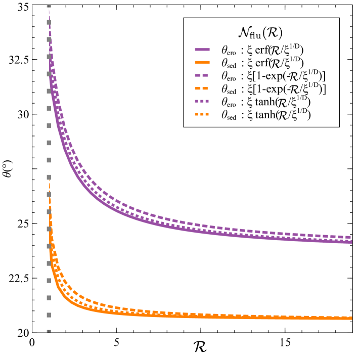
Figure S1: Predictions of the sedimentation angle $\theta_{\textrm{sed}}$ and erosion angle $\theta_{\textrm{ero}}$ as functions of the fluid-layer thickness $\mathcal{R}$ (in grain-diameter unit), through solutions of Eqs. (6) and (7) in the main text, for three different functional forms for the $\mathcal{N}_{\textrm{flu}}(\mathcal{R})$ ansatz, as indicated. In the model, the parameters are $\mu_{\textrm{eff}}=\tan(20^{\circ})$, $a=0.5$, $\varphi_{\textrm{sol}}=23.4^{\circ}$, $\xi=4.7$ and $D=0.94$ (see main text). The vertical dashed line indicates $\mathcal{R}=1$.

III Numerical simulations

Discrete Element Method (DEM) numerical simulations were performed with the software LIGGGHTS Kloss2012 . The simulated granular media were made of identical spherical beads with a $d=1$ mm diameter. The Hertz-Mindlin model was used to characterize the contacts between grains HertzMindlin . The following micromechanical parameters were chosen in order to reproduce the macroscopic behaviour of realistic granular media: $0.5$ restitution coefficient, $\mu_{\textrm{S}}=0.5$ bead-bead sliding friction coefficient, $\mu_{\textrm{R}}=0.01$ bead-bead rolling friction coefficient, as well as $1$ MPa Young’s modulus and $0.45$ Poisson ratio of the beads. In particular, both friction coefficients, $\mu_{\textrm{S}}$ and $\mu_{\textrm{R}}$, have been fixed in order to quantitatively reproduce the experimental results for spherical glass beads flowing down an inclined plane Pouliquen1999 . The effective friction coefficient $\mu_{\textrm{eff}}$ of the granular medium is obtained by considering that $\mu_{\textrm{eff}}=\tan[\theta_{\textrm{stop}}(\mathcal{R}\rightarrow\infty)]\approx\tan(20^{\circ})$.

For the inclined-plane configuration, we investigate the dependence of the stop angle with the fluid-phase thickness Pouliquen1999 ; Silbert2001 . We use a rectangular channel of 100$d$ height, 100$d$ length and 20$d$ width, filled with a layer of beads of thickness $\mathcal{R}$ (in unit of $d$ and counted vertically). Periodic boundary conditions are applied along both length and width directions. The plane is first inclined at an angle of 35^∘, in order to set the layer into motion, and then the angle is rapidly fixed at a lower value $\theta$. After the system has reached a steady flowing state, the angle is then reduced again progressively until the flowing layer stops – at the stop angle. In practice, the inclination is adjusted by artificially changing the direction of gravity.

For the heap configuration, we quantify the fluid-phase thickness $\mathcal{R}$ and the angle $\theta_{\textrm{heap}}$ of the fluid-solid interface, in the steady state, for different externally-imposed flow rates $Q$. A rectangular box of 400$d$ height, 400$d$ length and 20$d$ width is initially filled with beads. Periodic boundary conditions along the width direction are applied. A slope appears due to the sudden removal of the wall at $x=400d$. A continuous refill starts at the top (see Fig. 3(b) in the main text) in order to compensate for the continuous loss of grains at the bottom exit. The simulation is ran until a steady state is reached. The system self-adjusts its thickness $\mathcal{R}$ and angle $\theta_{\textrm{heap}}$ for a given value of the flow rate $Q$. It should be emphasized that obtaining reliable measurements in DEM simulations can be difficult for the heap configuration. First, there is a drastic influence of lateral walls Jop2005 , avoided here thanks to periodic lateral boundary conditions. Secondly, producing stationary flows down a heap requires very large systems. A large enough, 20$d$ wide, box is chosen in order to avoid any correlation due to the periodic boundary conditions. Moreover, as shown in Fig. S2, the length of the simulation box is also very important. Indeed, the observed heap angle $\theta_{\textrm{heap}}$ depends on the box length. For the systems studied here, we observed a saturation starting around a 300$d$ box length. Accordingly, we confidently chose a box with a 400$d$ length in order to avoid any effect of the box length. Thirdly, as previously suggested Orpe2004 ; Orpe2007 , the self-adjusted fluid-layer thickness is only estimated through the position of the inflexion point in the velocity profile related to the solid-fluid crossover. Finally, as previously shown Lemieux2000 , stationary flows cannot be obtained for the thinnest layers ($\mathcal{R}\lesssim 5$) in the heap configuration, as intermittent, unstable flows are instead observed.

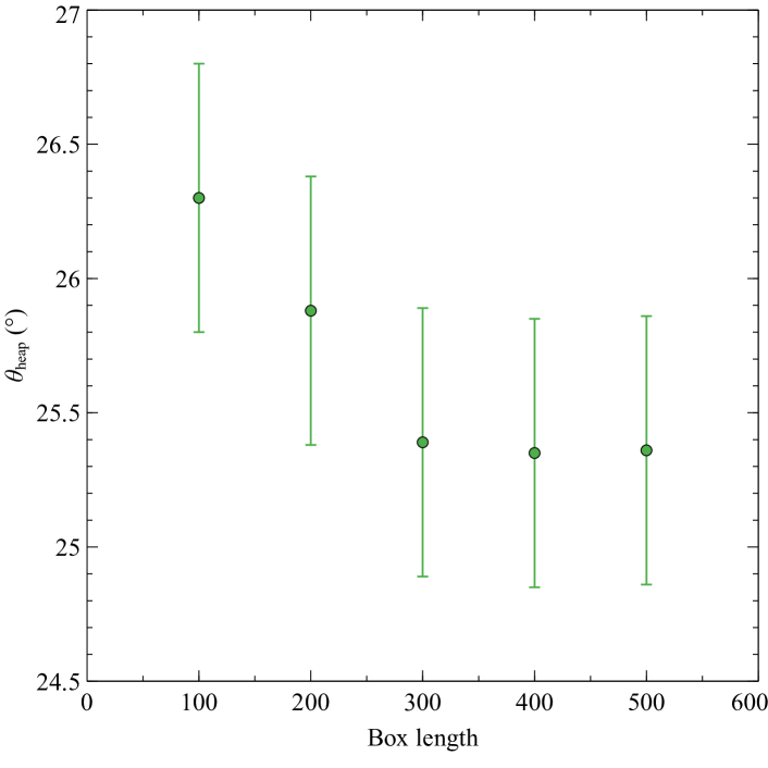
Figure S2: Heap angle $\theta_{\textrm{heap}}$ as a function of simulation box length (in grain-diameter unit), from DEM simulations in the heap configuration with a flow rate $Q=21000$ grains/s.

References

- (1) C. Kloss, C. Goniva, A. Hager, S. Amberger, S. Pirker. Models, algorithms and validation for opensource DEM andCFD-DEM Prog. Comput. Fluid Dyn. 12, 140-152 (2012).
- (2) LIGGGHTS(R)-PUBLIC Documentation, Version 3.X, DCS Computing GmbH, JKU Linz and Sandia Corporation. (2016). at https://www.cfdem.com/media/DEM/docu/gran_model_ hertz.html
- (3) O. Pouliquen Scaling laws in granular flows down rough inclined planes Phys. Fluids 11, 542 (1999).
- (4) L.E. Silbert, D. Ertaş, G.S. Grest, T.C. Halsey, D. Levine and S.J. Plimpton Granular flow down an inclined plane: Bagnold scaling and rheology Phys. Rev. E 64, 5-051302 (2001)
- (5) Pierre, J., Forterre, Y. & Pouliquen, O. Crucial role of sidewalls in granular surface flows: Consequences for the rheology. J. Fluid Mech. 541, 167-192 (2005).
- (6) A.V. Orpe and D.V. Khakhar Solid-Fluid Transition in a Granular Shear Flow Phys. Rev. Lett. 93, 6 - 068001 (2004)
- (7) A.V. Orpe and D.V. Khakhar Rheology of surface granular flows J. Fluid Mech. 571,1-32 (2007)
- (8) Lemieux, P.A. & Durian, D.J. From avalanches to fluid flow: A continuous picture of grain dynamics down a heap. Phys. Rev. Lett. 85, 4273–4276 (2000).