COSMOS: Coordination of High-Level Synthesis
and Memory Optimization for Hardware Accelerators

Abstract.

Hardware accelerators are key to the efficiency and performance of system-on-chip (SoC) architectures. With high-level synthesis (HLS), designers can easily obtain several performance-cost trade-off implementations for each component of a complex hardware accelerator. However, navigating this design space in search of the Pareto-optimal implementations at the system level is a hard optimization task. We present COSMOS, an automatic methodology for the design-space exploration (DSE) of complex accelerators, that coordinates both HLS and memory optimization tools in a compositional way. First, thanks to the co-design of datapath and memory, COSMOS produces a large set of Pareto-optimal implementations for each component of the accelerator. Then, COSMOS leverages compositional design techniques to quickly converge to the desired trade-off point between cost and performance at the system level. When applied to the system-level design (SLD) of an accelerator for wide-area motion imagery (WAMI), COSMOS explores the design space as completely as an exhaustive search, but it reduces the number of invocations to the HLS tool by up to 14.6$\times$.

1. Introduction

High-performance systems-on-chip (SoCs) are increasingly based on heterogeneous architectures that combine general-purpose processor cores and specialized hardware accelerators (Borkar and Chien, 2011; Horowitz, 2014; Carloni, 2016). Accelerators are hardware devices designed to perform specific functions. Accelerators are become popular because they guarantee considerable gains in both performance and energy efficiency with respect to the corresponding software executions (Chen et al., 2014; Cong et al., 2014; Zhang et al., 2015; Liu et al., 2016; Reagen et al., 2016; Kim, 2017; Chen et al., 2017; Ham et al., 2016). However, the integration of several specialized hardware blocks into a complex accelerator is a difficult design and verification task. In response to this challenge, we advocate the application of two key principles. First, to cope with the increasing complexity of SoCs and accelerators, most of the design effort should move away from the familiar register-transfer level (RTL) by embracing system-level design (SLD) (Sangiovanni-Vincentelli, 2007; Gerstlauer et al., 2009) with high-level synthesis (HLS) (Meeus et al., 2012; Qamar et al., 2017). Second, it is necessary to create reusable and flexible components, also known as intellectual property (IP) blocks, which can be easily (re)used across a variety of architectures with different targets for performance and metrics for cost.

1.1. System-Level Design

SLD has been proposed as a viable approach to cope with the increasing complexity of today architectures (Sangiovanni-Vincentelli, 2007; Gerstlauer et al., 2009). The SoC complexity is growing as a result of integrating a larger number of heterogeneous accelerators on the same chip. Further, accelerators are themselves becoming more complex to meet the high-performance and low-power requirements of emerging applications, e.g, deep-learning applications (Zhang et al., 2015; Reagen et al., 2016; Kim, 2017; Chen et al., 2017). To address the complexity of systems and accelerators, SLD aims at raising the level of abstraction of hardware design by replacing cycle-accurate low-level specifications (i.e., RTL Verilog or VHDL code) with untimed or transaction-based high-level specifications (i.e., C, C++ or SystemC code) (Qamar et al., 2017). This allows designers to focus on the relations between the data structures and computational kernels that characterize the accelerators, quickly evaluate different alternative implementations of the accelerators, and perform more complex and meaningful full-system simulations of the entire SoC. Indeed, designers can ignore low-level logic and circuit details that burden the design process. This improves the productivity and reduces the chances of errors (Carloni, 2016).

Unfortunately, current HLS tools are not ready yet to handle the complexity of today accelerators. Many accelerators are too complex to be synthesized by state-of-the-art HLS tools without being partitioned first. Accelerators must be decomposed into several computational blocks, or components, to be synthesized and explored efficiently. Decomposing an accelerator also helps improve the quality of results. Indeed, the choice of a particular RTL implementation for a component must be made in the context of the choices for all the other accelerator components. A particular set of choices leads to one point in the multi-objective design space of the accelerator. Thus, the process of deriving the diagram of Pareto-optimal points repeats itself hierarchically from the single component to the entire accelerator. This complexity is not handled by current HLS tools that optimize the single components independently from the others.

1.2. Intellectual Property Reuse

HLS supports IP block reuse and exchange. For instance, a team of computer-vision experts can devise an innovative algorithm for object recognition, design a specialized accelerator for this algorithm with a high-level language (C, C++, SystemC), and license it as a synthesizable IP block to different system architects; the architects can then exploit HLS tools to derive automatically the particular implementation that provides the best trade-off point (e.g., higher performance or lower area/power) for their particular system. The main idea of HLS is to raise the abstraction level of the design process to allow designers to generate multiple RTL implementations that can be reused across many different architectures. To obtain such a variety of implementations, the designers can change high-level configuration options, known as knobs, so that HLS can transform automatically the high-level specification of the accelerator and obtain several RTL implementations with different performance figures and implementation costs. For example, loop unrolling is a knob that allows designers to replicate parts of the logic to distribute computation in space (resource replication), rather than in time. The application of this knob generally leads to a faster, but larger, implementation of the initial specification.

Despite the advantages of HLS, performing this design-space exploration (DSE) is still a complicated task, especially for complex hardware accelerators. First, the support for memory generation and optimization is limited in current HLS tools. Some HLS tools still require third-party generators to provide a description of the memory organization and automatize the DSE process (Pilato et al., 2014, 2017). Several studies, however, highlight the importance of private memories to sustain the parallel datapath of accelerators: on a typical accelerator design, memory takes from 40% to 90% of the area (Lyons et al., 2012; Cota et al., 2015); hence, its optimization cannot be an independent task. Second, HLS tools are based on heuristics, whose behavior is not robust and often hard to predict (Kurra et al., 2007). Small changes to the knobs, e.g., changing the number of iterations unrolled in a loop, can cause significant and unexpected modifications at the implementation level. This increases the DSE effort because small changes to the knobs can take the exploration far from the Pareto-optimality.

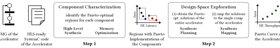
Figure 1. COSMOS: a methodology to coordinate HLS and memory optimization for the DSE of hardware accelerators.

1.3. Contributions

To address these limitations, we present COSMOS : an automatic methodology for the DSE of complex hardware accelerators, which are composed of several components. COSMOS is based on a compositional approach that coordinates both HLS tools and memory generators. First, thanks to the datapath and memory co-design, COSMOS produces a large set of Pareto-optimal implementations for each component, thus increasing both performance and cost spans. These spans are defined as the ratios between the maximum value and the minimum value for performance and cost, respectively. Second, COSMOS leverages compositional design techniques to significantly reduce the number of invocations to the HLS tool and the memory generator. In this way, COSMOS focuses on the most critical components of the accelerator and quickly converges to the desired trade-off point between cost and performance for the entire accelerator. The COSMOS methodology consists of two main steps (Figure 1). First, COSMOS uses an algorithm to characterize each component of the accelerator individually by efficiently coordinating multiple runs of the HLS and memory generator tools. This algorithm finds the regions in the design space of the components that include the Pareto-optimal implementations (Component Characterization in Figure 1). Second, COSMOS performs a DSE to identify the Pareto-optimal solutions for the entire accelerator by efficiently solving a linear programming (LP) problem instance (Design-Space Exploration).

We evaluate the effectiveness and efficiency of the COSMOS methodology on a complex accelerator for wide-area motion imagery (WAMI) (Porter et al., 2010; Barker et al., 2013), which consists of approximately 7000 lines of SystemC code. While exploring the design space of WAMI, COSMOS returns an average performance span of 4.1$\times$ and an average area span of 2.6$\times$, as opposed to 1.7$\times$ and 1.2$\times$ when memory optimization is not considered and only standard dual-port memories are used. Further, COSMOS achieves the target data-processing throughput for the WAMI accelerator while reducing the number of invocations to the HLS tool per component by up to 14.6$\times$, with respect to an exhaustive exploration approach.

1.4. Organization

The paper is organized as follows. Section 2 provides the necessary background for the rest of the paper. Section 3 describes few examples to show the effort required in the DSE process. Section 4 gives an overview of the COSMOS methodology, which is then detailed in Sections 5 (Component Characterization) and 6 (Design-Space Exploration). Section 7 presents the experimental results. Section 8 discusses the related work. Finally, Section 9 concludes the paper.

2. Preliminaries

This section provides the necessary background concepts. We first describe the main characteristics of the accelerators targeted by COSMOS in Section  2.1. Then, we present the computational model we adopt for the DSE in Section 2.2.

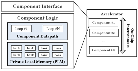
Figure 2. Architecture of a loosely-coupled accelerator.

2.1. Hardware Accelerators

Several accelerator designs have been proposed in the literature to realize hardware implementations that execute important computational kernels more efficiently than corresponding software executions (Chen et al., 2014; Zhang et al., 2015; Liu et al., 2016; Reagen et al., 2016; Kim, 2017; Chen et al., 2017). The accelerators can be located either inside (tightly-coupled) or outside (loosely-coupled) the processing cores (Cota et al., 2015). The former class of accelerators is more suitable for fine-grain computations on small data sets, while the latter is better for coarse-grain computations on large data sets. We focus on loosely-coupled accelerators in this paper because the complexity of their design requires a compositional approach. WAMI is representative of a set of classes of applications that can be benefit from the adoption of the loosely-coupled accelerator model and a compositional design approach.

Architecture

We design our accelerators in SystemC. Figure 2 illustrates their typical architecture. They are made of multiple components that are designed individually to cope with the current limitations of HLS tools in optimizing complex components. Partitioning the accelerators into multiple components allows HLS tools to handle them separately, thus reducing the synthesis time and improving the quality of results. Each component is specified as a separated SystemC module and represents a computational block within the accelerator. The components communicate by exchanging the data through an on-chip interconnect network that implements transaction-level modeling (TLM) (Ghenassia, 2006) channels. These channels synchronize the components by absorbing the potential differences in their computational latencies with a latency-insensitive communication protocol (Carloni, 2015). This ensures that the components of an accelerator can always be replaced with different Pareto-optimal implementations without affecting the correctness of the accelerator implementation. COSMOS employs channels with a fixed bitwidth (256 bits) and does not explore different design alternatives to implement the communication among the components. It can be extended, however, to support this type of DSE by using, for example, the XKnobs (Piccolboni et al., 2017) or buffer-restructuring techniques (Cong et al., 2017). Each component includes a datapath, which is organized in a set of loops, to read and store input and output data and to compute the required functionality. There are also private local memories (PLMs), or scratchpads, where data resides during the computation. PLMs are multi-bank memory architectures that provide multiple read and write ports to allow accelerators to perform parallel accesses. We generate optimized memories for our accelerators by using the Mnemosyne memory generator (Pilato et al., 2017). Several analyses highlight the importance of the PLMs in sustaining the parallel datapath of accelerators (Lyons et al., 2012; Cota et al., 2015). PLMs play a key role on the performance of accelerators (Li et al., 2011), and they occupy from 40% to 90% of the entire area of the components of a given accelerator (Lyons et al., 2012).

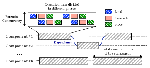
Figure 3. Execution of a loosely-coupled accelerator.

Execution

Figure 3 reports an example of execution of an accelerator made of multiple components. The execution of each component of the accelerator is divided in three phases (showed on the top of the figure for Component #1). In the load phase the components communicate with the on-chip interconnect network to read the input data and store it in the PLMs. In the compute phase the components execute the given functions on the data currently stored in the PLMs. In the store phase the components communicate with the on-chip interconnect network to store the output data available in the PLMs. These three phases can be pipelined by using techniques such as ping-pong or circular buffers (Cota et al., 2015), as shown on the top of the figure. After having identified the minimum block of data that is sufficient to realize the required function in each component, e.g., a frame, the execution of the components can be: (i) completely overlapped when there are no dependencies (e.g., Component #1 and #K), or (ii) serialized when a component needs input data from another component to start its computation (e.g., Component #1 and #2).

2.2. Computational Model

To formally model the loosely-coupled accelerators we use timed marked graphs (TMGs), a subclass of Petri nets (PNs) (Murata, 1989). TMGs are commonly used to perform compositional performance analysis of discrete-event systems (Campos et al., 1992). While TMGs do not allow to capture data-dependent behaviors, they are a practical model to analyze stream processing accelerators for many classes of applications, e.g., image and signal processing applications. A PN is a bipartite graph defined as a tuple $(P,T,F,w,M_{0})$, where $P$ is a set of $m$ places, $T$ is a set of $n$ transitions, $F:(P\times T)\cup(T\times P)$ is a set of arcs, $w:F\to\mathbb{N}^{+}$ is an arc weighting function, and $M_{0}\in\mathbb{N}^{m}$ is the initial marking, i.e. the number of tokens at each $p\in P$. A PN is strongly-connected if for every pairs of places $p_{i}$ and $p_{j}$ there exists a sequence of transitions and places such that $p_{i}$ and $p_{j}$ are mutually reachable in the net. A PN can be organized in a set of strongly-connect components, i.e., the maximal sets of places that are strongly-connected. A TMG is a PN such that (i) each place has exactly one input and one output transition, and (ii) $w:F\to 1$, i.e., every arc has a weight equal to $1$. To measure performance, TMGs are extended with a transition firing-delay vector $\tau\in\mathbb{R}^{n}$, which represents the duration of each particular firing.

The minimum cycle time of a strongly-connected TMG is defined as: ${max}\ \{D_{k}/N_{k}\mid k\in K\}$, where $K$ is the set of cycles of the TMG, $D_{k}$ is the sum of the transition firing delays in cycle $k$, and $N_{k}$ is the number of tokens in cycle $k$ (Ramamoorthy and Ho, 1980). In this paper, we use the TMG model to formally describe the accelerators. We use the term system to indicate a complex accelerator that is made of multiple components. Each component of the system is represented with a transition in the TMG whose firing delay is equal to its effective latency. The effective latency $\lambda$ of a component is defined as the product of its clock cycle count and target clock period. The maximum sustainable effective throughput $\theta$ of the system is then the reciprocal of the minimum cycle time of its TMG, if the TMG is strongly connected. Otherwise, it is the minimum $\theta$ among its strongly-connected components. We use $\lambda$ and $\theta$ as performance figures for the single components and the system, respectively. We use the area $\alpha$ as the cost metric for both the components and the system.

3. Motivational Examples

Performing an accurate and as exhaustive as possible DSE for a complex hardware accelerator is a difficult task for three main reasons: (i) HLS tools do not always support PLM generation and optimization (Section 3.1), (ii) HLS tools are based on heuristics that make it difficult to configure the knobs (Section 3.2), and (iii) HLS tools do not handle the simultaneous optimization of multiple components (Section 3.3). Next, we detail these issues with some examples.

3.1. Memories

The joint optimization of the accelerator datapath and PLM architecture is critical for an effective DSE. Figure 4 depicts the design space of Gradient, a component we designed for WAMI. The graph reports different design points, each characterized in terms of area (mm²) and effective latency (milliseconds), synthesized for an industrial 32nm ASIC technology library. The points with the same color (shape) are obtained by partially unrolling the loops for different numbers of iterations. The different colors (shapes) indicate different numbers of ports for the PLM. By increasing the number of ports, we notice a significant impact on both latency and area. In fact, multiple ports allow the component to read and write more data in the same clock cycle, thus increasing the hardware parallelism. Multi-port memories, however, require much more area since more banks may be used depending on the given memory-access pattern. Note that ignoring the role of the PLM limits considerably the design space. By changing the number of ports of the PLM, we obtain a latency span of $7.9\times$ and an area span of $3.7\times$. By using standard dual-port memories, we have only a latency span of $1.4\times$ and an area span of $1.2\times$. This motivates the need of considering the optimization of PLMs in the DSE process. COSMOS takes into consideration the PLMs by generating optimized memories with Mnemosyne (Pilato et al., 2017).

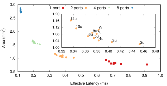
Figure 4. Example of application of two HLS knobs (number of ports, number of unrolls) to Gradient, a component of WAMI. The nested graph magnifies the design points with 2 read and 2 write ports. The numbers indicate the numbers of iterations unrolled.

3.2. HLS Unpredictability

Dealing with the unpredictability of the HLS tool outcomes is necessary to remain in the Pareto-optimal regions of the design space (Kurra et al., 2007). This is highlighted by the magnified graph in Figure 4 that reports the number of iterations unrolled for each design point of Gradient. By increasing the number of iterations unrolled in a loop for a particular configuration of the PLM ports we expect to obtain design points that have more area and less latency. In fact, unrolling a loop increases the number of hardware resources to allow more parallel operations. However, an effective parallelization is not always guaranteed. Some combinations of loop unrolling have a negative effect on both latency and area due to the applications of HLS heuristics (e.g., points $7$u, $8$u and $9$u in Figure 4). In fact, HLS tools need to insert additional clock cycles in the body of a loop when (i) operation dependencies are present or (ii) the area is growing too much with respect to the scheduling metrics they adopt (HLS tools often perform latency-constrained optimizations to minimize the area). This motivates the need of dealing with the HLS unpredictability in the DSE process. COSMOS applies synthesis constraints to account for the high variability and partial unpredictability of the HLS tools.

3.3. Compositionality

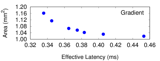
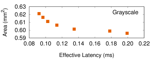
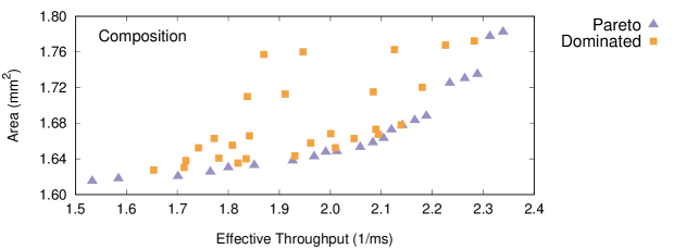
Figure 5. Example of composition for Gradient and Grayscale, two components of WAMI. The graphs on the top report some Pareto-optimal points for the two components. The graph on the bottom shows all the possible combinations of these components, assuming they are executed sequentially in a loop. In the graph of the composition, the effective throughput is used as the performance metric.

Complex accelerators need to be partitioned into multiple components to be efficiently synthesized by current HLS tools. This reduces the synthesis time and improves the quality of results, but significantly increases the DSE effort. Figure 5 reports a simple example to illustrate this problem. On the top, the figure reports two graphs representing a small subset of Pareto-optimal points for Gradient and Grayscale, two components of WAMI. Assuming that they are executed sequentially in a loop, their aggregate throughput is the reciprocal of the sum of their latencies. On the bottom, the figure reports all the possible combinations of the design points of the two components, differentiating the Pareto-optimal combinations from the Pareto-dominated combinations. These design points are characterized in terms of area (mm²) and effective throughput (1/milliseconds). In order to find the Pareto-optimal combinations at the system level, an exhaustive search method would apply the following steps: (i) synthesize different points for each component by varying the settings of the knobs, (ii) find the Pareto-optimal points for each component, and (iii) find the Pareto-optimal combinations of the components at the system level. This approach is impractical for complex accelerators. First, step (i) requires to try all the combinations of the knob settings (e.g., different number of ports and number of unrolls). Second, step (iii) requires to evaluate an exponential number of combinations at the system level to find those that are Pareto-optimal. In fact, if we have $n$ components with $k$ Pareto-optimal points each, then the number of combinations to check is $\mathcal{O}(k^{n})$. This example motivates the need of a smart compositional method that identifies the most critical components of an accelerator and minimizes the invocations to the HLS tool. In order to do that, COSMOS reduces the number of combinations of knob settings that are used for synthesis and prioritizes the synthesis of the components depending on their level of contribution to the effective throughput of the entire accelerator.

4. The COSMOS Methodology

As shown in Figure 1, COSMOS consists of the following steps:

1. Component Characterization (Section 5): in this step COSMOS analyzes each component of the system individually; for each component it identifies the boundaries of the regions that include the Pareto-optimal designs; starting from the HLS-ready implementation of each component (in SystemC), COSMOS applies an algorithm that generates knob and memory configurations to automatically coordinate the HLS and memory generator tools; the algorithm takes into account the memories of the accelerators and tries to deal with the unpredictability of HLS tools;

2. Design-Space Exploration (Section 6): in this step COSMOS analyzes the design space of the entire system; the system is modeled with a TMG to find the most critical components for the system throughput; then, COSMOS:

   • formulates a LP problem instance to identify the latency requirements of each component that ensure the specified system throughput and minimize the system cost; this step is called Synthesis Planning (Section 6.1);

   • maps the solutions of the LP problem to the knob-setting space of each component and runs additional synthesis to get the RTL implementations of the components; this step is called Synthesis Mapping (Section 6.2).

5. Component Characterization

Algorithm 1 reports the pseudocode used for the component characterization. The designer provides the clock period, the maximum number of ports for the PLMs (mainly constrained by the target technology and the memory generator) and the maximum number of loop unrolls. In order to keep the delay of the logic for selecting the memory banks negligible, the number of ports should be a power of two. Note that this constraint can be partially relaxed without requiring Euclidean division for the selection logic (Seznec, 2015). The number of unrolls depends on the loop complexity. Loops with few iterations can be completely unrolled, while more complex loops can be only partially unrolled. In fact, unrolling loops replicates the hardware resources, thus making the scheduling more complex for the HLS tool. The algorithm identifies regions in the design space of the component. A region includes design points that have the same number of ports. They are bounded by an upper-left ($\lambda_{min},\alpha_{max}$) and a lower-right ($\lambda_{max},\alpha_{min}$) point. These regions represent the design space of the component that will be used for the DSE at the system level, as explained in Section 6.

Input: $clock$, $max\_ports$, $max\_unrolls$

Output: set of regions $(\lambda_{max},\alpha_{min},\lambda_{min},\alpha_{max})$

1

2 

3for ports = 1 up to $max\_ports$ do

      3 // Identification of max-$\lambda$ min-$\alpha$ point

4       $(\lambda_{max},\alpha_{min})$ = hls_tool(ports, ports, $clock$);

      4 // Identification of min-$\lambda$ max-$\alpha$ point

5       for unrolls = $max\_unrolls$ down to ports + 1 do

6             $(\lambda_{min},\alpha_{max})$ = hls_tool(unrolls, ports, $clock$);

7             if $\lambda$_constraint${}_{\text{{ports}}}$(unrolls) is sat then break;

8            

      8// Generation of the PLM of the component

9       $\alpha_{plm}$ = memory_generator(ports);

10       $\alpha_{min}$ += $\alpha_{plm}$;  $\alpha_{max}$ += $\alpha_{plm}$;

      10 // Save the region of the design space

11       $save$($ports,unrolls,\lambda_{max},\alpha_{min},\lambda_{min},\alpha_{max}$);

12      

13 

tool parameters: hls_tool(unrolls, ports, clock);

tool parameters: memory_generator(ports);

Algorithm 1 Component Characterization

Algorithm 1 starts by identifying the lower-right point of the region. To identify this design point, it sets the number of unrolls equal to the current number of ports (line 3). This ensures that all the ports of the PLM are exploited and the obtained point is not redundant. In fact, this point cannot be obtained by using a lower number of ports. On the other hand, finding the upper-left point is more challenging. A complete unroll (which could lead to the point with the minimum latency) is unfeasible in case of complex loops. Indeed, it is not always guaranteed that, by increasing the number of unrolls, the HLS tool returns an implementation of the component that gives lower latency in exchange for higher area occupation. To overcome these problems, Algorithm 1 introduces a constraint, $\lambda-constraint$ for the rest of the paper, that defines the maximum number of states that the HLS tool can insert in the body of a loop. This helps in constraining the behavior of the HLS tool to be more deterministic and in removing some of the Pareto-dominated points. Thus, Algorithm 1 uses the following function to estimate the number of states that should be sufficient to schedule one iteration of the loop that includes read and write operations:

(1) $$h_{ports}(unrolls)=\left\lceil\frac{\gamma_{r}*unrolls}{ports}\right\rceil+\left\lceil\frac{\gamma_{w}}{ports}\right\rceil+\eta$$

where $\gamma_{r}$ is the maximum number of read accesses to the same array per loop iteration, $\gamma_{w}$ is the maximum number of write accesses to the same array per loop iteration and, $\eta$ accounts for the latency required to perform the operations that do not access the PLM. These parameters are inferred by traversing the control data flow graph (CDFG) created by the HLS tool for scheduling the lower-right point. This function is used as an upper bound of the number of states that the HLS tool can insert. If this upper bound is not sufficient, then the synthesis fails and the point is discarded. A synthesis run with a lower number of unrolls is performed to find another point to be used as the upper-left extreme (lines 5-7).

Example 1.

Figure 6 shows an example of using the $\lambda$-constraint. The loop (reported on the left) contains two read operations to two distinct arrays, i.e., $\gamma_{r}=1$, and one write operation, i.e., $\gamma_{w}=1$. We assume that all the operations that are neither read nor write operations can be performed in one clock cycle, i.e., $\eta=1$. The two diagrams (on the right) show the results of the scheduling by using two ports for the PLM and by unrolling two or three times the loop, respectively. In the first case (unrolls = 2), the HLS tool can schedule all the operations in a maximum of $h_{2}(2)=3$ clock cycles. Thus, this point would be chosen by Algorithm 1 to be used as upper-left extreme. In the second case (unrolls = 3), the HLS tool is not able to complete the schedule within $h_{2}(3)=4$ clock cycles (it needs at least 5 clock cycles). Thus, this point is discarded.

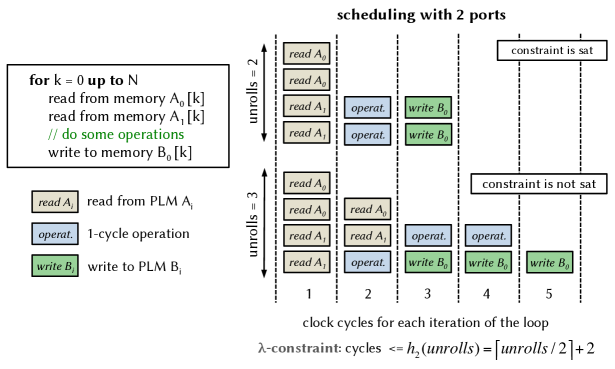
Figure 6. Example of application of the $\lambda$-constraint.

Note that the $\lambda$-constraint is not guaranteed to obtain a Pareto-optimal point due to the intrinsic variability of the HLS results. Still, this point can serve as an upper bound of the region in the design space. Note also that the $\lambda-constraint$ cannot be applied to loops that (i) require data from sub-components through blocking interfaces or (ii) do not present memory accesses to the PLM. In these cases, in fact, it is necessary to extend the definition of the estimation function given in Equation (1) to handle such situations. Alternatively, COSMOS can optionally run some synthesis in the neighbourhood of the maximum number of unrolls and use a local Pareto-optimal point as the upper-left extreme.

5.1. Memory Generation

After the two extreme points of a region have been determined, the algorithm instructs the memory generator to create the PLM architecture (line 9). COSMOS uses Mnemosyne (Pilato et al., 2017) to generate optimized PLMs for the components. Mnemosyne has been integrated with the commercial HLS tool we use for the experimental results (Section 7). The CDFG, created by the HLS tool, is analyzed to find the arrays specified in the code and their access patterns. Then, a memory is generated according to these specifications and the area required for the PLM is added to the logic area reported by the HLS tool (line 10). The memory architecture is tailored to the component needs and is optimized with respect to the required number of ports and access patterns. In particular, given a certain number of ports, Mnemosyne combines several SRAMs, or BRAMSs in case of FPGA devices, into a multi-bank architecture (Figure 2). Each SRAM (BRAM) provides 2 read/write ports, thus by combining them in a multi-bank architecture Mnemosyne allows the component to perform multiple accesses in parallel (Baradaran and Diniz, 2008).

6. Design-Space Exploration

After the characterization of the single components of a given accelerator, COSMOS uses a LP formulation to find the Pareto-optimal design points at the system level. The DSE problem at the system level can be formulated as follows:

Problem 1.

Given a TMG model of the system where each component has been characterized, a HLS tool, and a target granularity $\delta>0$, find a Pareto curve $\alpha$ versus $\theta$ of the system, such that:

1. given two consecutive points $d$, $d^{\prime}$ on the Pareto curve, they have to satisfy: $max\ \{d_{\alpha}^{\prime}/d_{\alpha}-1,d_{\theta}^{\prime}/d_{\theta}-1\}<\delta$; this ensures a maximum distance between two design points on the curve;

2. the HLS tool must be invoked as few times as possible.

This formulation is borrowed from (Liu et al., 2012), where the authors propose a solution that requires the manual effort of the designers to characterize the components. In contrast, COSMOS solves this problem by leveraging the automatic characterization method in Section 5 and by dividing it into two steps: Synthesis Planning and Synthesis Mapping.

6.1. Synthesis Planning

Given a strongly-connected system TMG, COSMOS uses the following $\theta$-constrained cost-minimization LP formulation:

(2) $$\begin{array}[]{rl}$min$&\sum_{i=1}^{n}f_{i}(\tau_{i})\\ \mbox{s.t.}&A\sigma+M_{0}/\theta\geq\tau^{-}\\ &\tau_{min}^{-}\leq\tau^{-}\leq\tau_{max}^{-}\end{array}$$

where the function $f_{i}$ returns the implementation cost ($\alpha$) of the $i$-th component given the firing-delay $\tau_{i}$ of transition $t_{i}$, $\sigma\in\mathbb{R}^{n}$ is the transition-firing initiation-time vector, $M_{0}\in\mathbb{N}^{m}$ is the initial marking, $\tau^{-}\in\mathbb{R}^{m}$ is the input-transition firing-delay vector, i.e., $\tau_{i}^{-}$ is the firing-delay of the transition $t_{k}$ entering in place $p_{i}$ (note that $\tau_{min}^{-}$ and $\tau_{max}^{-}$ correspond to the extreme $\lambda_{min}$ and $\lambda_{max}$ of the components), and $A$ is the ${m\times n}$ incidence matrix defined as:

(3) $$A[i,j]=\left\{\begin{array}[]{l l}+1&\quad\text{if $t_{j}$ is an output transition of $p_{i}$,}\\ -1&\quad\text{if $t_{j}$ is an input transition of $p_{i}$,}\\ 0&\quad\text{otherwise.}\\ \end{array}\right.$$

The objective function minimizes the implementation costs of the components, while satisfying the system throughput requirements. Given the component extreme latencies $\lambda_{min}$ and $\lambda_{max}$, it is possible to determine the values of $\theta_{min}$ and $\theta_{max}$ by labeling the transitions of the TMG of the system with such latencies. By iterating from $\theta_{min}$ to $\theta_{max}$ with a ratio of $(1+\delta)$, we can then find the optimal values of $\lambda$ for the components that solve Problem 1. This formulation guarantees that the components that are not critical for the system throughput are selected to minimize their cost. The cost functions $f_{i}$ in Equation (2) are unknown a-priori, but they can be approximated with convex piecewise-linear functions. This LP formulation can be solved in polynomial time (Boyd and Vandenberghe, 2004), and it can be extended to the case of non-strongly-connected TMGs.

6.2. Synthesis Mapping

Given the optimal values of $\lambda$ of each component that solve Problem 1, it is necessary to determine the knob settings that provide the component implementations meeting such requirements. In other words, we need an inverse function $\phi$ that maps the optimal solutions $\lambda$ to the corresponding values in the knob-setting space of each component. The solutions of Equation (2) can require values of $\lambda$ for a component falling inside a certain region. Since we have only the component implementations for the extreme points of the region (synthesized with Algorithm 1), we need to find the knob settings that return also the intermediate points. Given the $\lambda_{target}$ requirement of a component (from Equation (2)), COSMOS first finds the region (returned by Algorithm 1) in which $\lambda_{target}$ falls, i.e., $\lambda_{target}\in[\lambda_{min},\lambda_{max}]$. Then, since every region includes design points that have the same number of ports, COSMOS needs only to estimate the number of unrolls to generate a proper knob setting. To do that, COSMOS uses the following modified version of Amdahl’s Law (Amdahl, 1967):

(4) $$\frac{\lambda_{target}}{\lambda_{max}}=\frac{1}{(1-\frac{\mu_{target}-\mu_{min}}{\mu_{max}-\mu_{min}})+\frac{\mu_{target}-\mu_{min}}{\mu_{max}-\mu_{min}}*\frac{\lambda_{max}}{\lambda_{min}}}$$

where $\mu_{target}$ is the estimated number of unrolls, while $\mu_{min}$, $\mu_{max}$ are the numbers of unrolls which correspond to $\lambda_{max}$ and $\lambda_{min}$, respectively. The only unknown term in this equation is $\mu_{target}$, i.e., the number of unrolls that can be used to satisfy the $\lambda_{target}$ requirement. Thus, COSMOS uses the following mapping function to map the $\lambda$ requirements to the effective number of unrolls:

(5) $$\begin{split}\mu_{target}&=\ \phi(\lambda_{target},\lambda_{min},\lambda_{max},\mu_{min},\mu_{max})=\\ &=\ \frac{\begin{multlined}(\lambda_{min}\lambda_{max}\mu_{max}+\lambda_{target}\lambda_{max}\mu_{min})\ -\\ (\lambda_{min}\lambda_{max}\mu_{min}+\lambda_{target}\lambda_{min}\mu_{max})\end{multlined}(\lambda_{min}\lambda_{max}\mu_{max}+\lambda_{target}\lambda_{max}\mu_{min})\ -\\ (\lambda_{min}\lambda_{max}\mu_{min}+\lambda_{target}\lambda_{min}\mu_{max})}{\lambda_{target}(\lambda_{max}-\lambda_{min})}\end{split}$$

This function is derived from Equation (4), and thus it models the law of diminishing returns. This provides a good approximation of the number of unrolls because, typically, the relative gains in latency keep decreasing as we increase the number of unrolls (Section 7). After generating the knob settings by using the mapping function, COSMOS runs the corresponding synthesis to get (i) the actual values for $\lambda$ and $\alpha$ and (ii) the RTL implementation of the component.

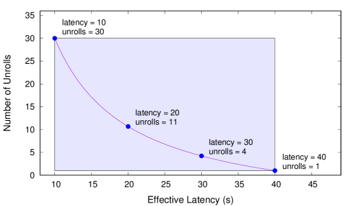
Figure 7. Example of application of the mapping function $\phi$.

Example 2.

Figure 7 shows an example of a mapping function. The lower-right point of the corresponding region has a latency of 40 s, while the upper-left point has a latency of 10 s, i.e. $\lambda_{max}$ = 40 s, $\lambda_{min}$ = 10 s. The lower-right point does not unroll the loops, while the other one unrolls the loops for 30 iterations, i.e., $\mu_{min}=1$, $\mu_{max}$ = 30. By using these parameters the graph plots the mapping function that returns the number of unrolls that should be applied, given a specific value for the latency (we apply the ceiling function to get an integer value). For instance, if a point with latency of 20 s is required, the mapping function returns 11 as the number of unrolls. Note that by specifying the maximum latency, the function returns the minimum number of unrolls, while by specifying the minimum latency, it returns the maximum number of unrolls.

It is possible that the mapping may fail by choosing a value for $\mu_{target}$ that does not satisfy the $\lambda$-constraint (Section 5). In this case, COSMOS tries to increase the number of unrolls to preserve the throughput. Further, if $\lambda_{target}$ is not included in any region, COSMOS uses the slowest point of the next region that has a larger number of ports. This does not require a synthesis run (because that point has been synthesized during the characterization), and it is a conservative solution because, as in the case of failure of the $\lambda$-constraint, we are willing to trade area to preserve the throughput.

7. Experimental Results

We implement the COSMOS methodology with a set of tools and scripts to automatize the DSE. Specifically, COSMOS includes: (i) Mnemosyne (Pilato et al., 2017) to generate multi-bank memory architectures as described in Section 5, (ii) a tool to extract the information required by Mnemosyne from the database of the HLS tool, (iii) a script to run the synthesis and the memory generator according to Algorithm 1, (iv) a program that creates and solves the LP model by using the GLPK Library (Section 6.1), and (v) a tool that maps the LP solutions to the HLS knobs and runs the synthesis (Section 6.2).

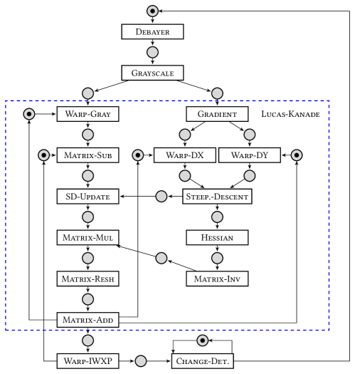
Figure 8. TMG modeling the WAMI application.

We evaluate the effectiveness and efficiency of COSMOS by considering the WAMI application (Porter et al., 2010) as a case study. The original specification of the WAMI application is available in C in the PERFECT Benchmark Suite (Barker et al., 2013). Starting from this specification, we design a SystemC accelerator to be synthesized with a commercial HLS tool, i.e., Cadence C-to-Silicon. We use an industrial $32$nm ASIC technology as target library. We choose the WAMI application as our case study due to (i) the different types of computational blocks it includes and (ii) its complexity. The heterogeneity of its computational blocks allows us to develop different components for each block and show the vast applicability of COSMOS. The C specification is roughly $1000$ lines of code. The specification of our accelerator design is roughly $7000$ lines of SystemC code.

7.1. Computational Model

We model the WAMI application as a loosely-coupled accelerator. Figure 8 illustrates the resulting TMG model of the accelerator. The WAMI specification includes four main components: (i) Debayer for image filtering, (ii) Grayscale for RGB-to-Grayscale color conversion, (iii) Lucas-Kanade for the image alignment, and (iv) the Change-Detection classifier. We partition Lucas-Kanade into many sub-components to further increase the hardware parallelism. Matrix-Inv is executed in software to preserve the floating-point precision. Therefore, it is modeled with a fixed effective latency during the DSE process.

7.2. Component Characterization

	COSMOS			No Memory
Component	$reg$	$\lambda_{span}$	$\alpha_{span}$	$\lambda_{span}$	$\alpha_{span}$
Debayer	3	$2.89\times$	$1.99\times$	$1.04\times$	$1.36\times$
Grayscale	4	$6.91\times$	$3.41\times$	$2.75\times$	$1.14\times$
Gradient	4	$7.89\times$	$3.65\times$	$1.39\times$	$1.22\times$
Hessian	4	$7.70\times$	$7.30\times$	$1.44\times$	$1.30\times$
SD-Update	4	$9.87\times$	$2.01\times$	$2.78\times$	$1.79\times$
Matrix-Sub	4	$2.75\times$	$3.98\times$	$1.88\times$	$1.05\times$
Matrix-Add	3	$1.53\times$	$1.01\times$	$1.26\times$	$1.01\times$
Matrix-Mul	3	$2.88\times$	$3.05\times$	$1.92\times$	$1.14\times$
Matrix-Resh	1	$1.02\times$	$1.04\times$	$1.02\times$	$1.04\times$
Steep.-Descent	1	$1.95\times$	$1.46\times$	$1.95\times$	$1.46\times$
Change-Det.	1	$2.21\times$	$1.04\times$	$2.21\times$	$1.04\times$
Warp	1	$1.09\times$	$1.03\times$	$1.09\times$	$1.03\times$
Average	-	$4.06\times$	$2.58\times$	$1.73\times$	$1.22\times$

Table 1. Characterization of the components for WAMI. The table reports the differences in latency ($\lambda$) and area ($\alpha$) span when memory is considered (COSMOS) or not (No Memory). For COSMOS, $reg$ indicates the number of regions found with Algorithm 1.

COSMOS applies Algorithm 1 (Section 5) to characterize the components of the system. Table 1 reports the results of the characterization for the WAMI accelerator: the algorithm used by COSMOS (COSMOS) is compared with the case in which memory is not considered in the characterization (No Memory). In the latter case, we assume to have only standard dual-port memories. For each component, the table reports the latency span ($\lambda_{span}$), i.e., the ratio between the maximum latency and the minimum latency, the area span ($\alpha_{span}$), i.e., the ratio between the maximum area and the minimum area. For COSMOS, the table shows also the total number of regions identified by the algorithm ($reg$). For Algorithm 1 we use a number of ports in the interval $[1,16]$ and a maximum number of unrolls in the interval $[8,32]$, depending on the components. COSMOS guarantees overall a richer DSE, as evidenced by the average results. For some components the algorithm extracts only one region because multiple ports can incur in additional area for no latency gains. This happens when (i) the algorithm cannot exploit multiple accesses in memory, or (ii) the data is cached into local registers which can be accessed in parallel in the same clock cycle, e.g., for Change-Detection. On the other hand, in most cases COSMOS provides significant gains in terms of area and latency spans compared to a DSE that does not consider the memories.

Figure 9 shows the design space of four representative components of WAMI. The rectangles in the figures are the regions found by Algorithm 1. For completeness, in addition to the design points corresponding to the extreme points of the regions, the graphs show also the intermediate points that could be selected by the mapping function. The small graphs on the right magnify the corresponding regions reported on the left. As in the examples discussed in Section 3, increasing the number of ports has a significant impact on the DSE, while loop unrolling has a local effect within each region. Another aspect that is common among many components is that the regions become smaller as we keep increasing the number of ports. For example, for Grayscale in Figure 9 (c), we note that by increasing the number of ports, we reach a point where the gain in latency is not significative. This effect, called diminishing returns (Amdahl, 1967), is the same effect that can be observed in the parallelization of software algorithms. In some cases, changing the ports increases only the area with no latency gains as discussed in the previous paragraph. This is highlighted in Figure 9 (d), where for Change-Detection we report two additional regions with respect to those specified in Table 1. The diminishing-return effect can also be observed by increasing the number of unrolls inside a region, e.g., Figure 9 (b). This is why COSMOS exploits Amdahl’s Law (Section 6.2). On the other hand, we notice some discontinuities of the Pareto-optimal points within some regions, e.g., the region in the bottom-right corner of Figure  9 (a). Even by applying the $\lambda-constraints$ (Section 5) it is not possible to completely discard the Pareto-dominated implementations. In fact, by further restricting the imposed constraints, i.e., by reducing the number of states that the HLS tool can insert in each loop, we observe that also the Pareto-optimal implementations are discarded. Thus, it is not always possible to obtain a curve composed only of Pareto-optimal points within a certain region. Finally, the Pareto-optimal points outside the regions are not discarded by COSMOS. They can be chosen when it is necessary to perform the mapping (Section 6.2).

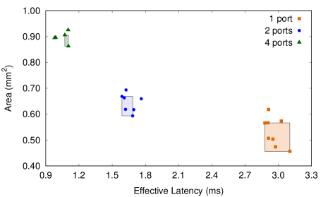
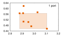
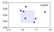
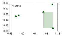
(a) Debayer

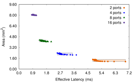
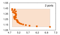
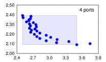
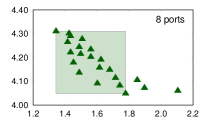
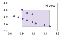
(b) Hessian

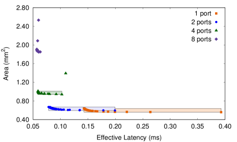
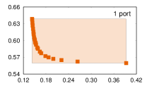
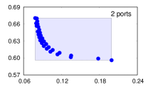
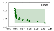
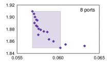
(c) Grayscale

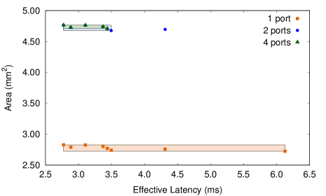
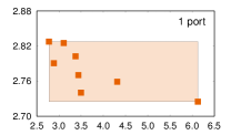
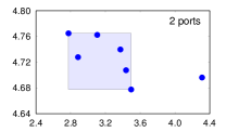
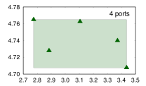
(d) Change-Det

Figure 9. Characterization of four representative components of the WAMI accelerator.

7.3. Design-Space Exploration

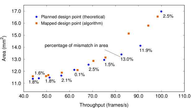
Figure 10. Results of the compositional DSE for WAMI.

After the characterization of the single components, COSMOS applies the DSE approach explained in Section 6. It first finds the optimal solutions at the system level by using Equation (2) (Section 6.1). It then applies the mapping function to determine the knob settings of the single components and runs the necessary synthesis (Section 6.2). Figure 10 shows the resulting Pareto curve that includes the planned points (from Equation (2)) and the mapped points (returned by the mapping function). These design points are characterized in terms of effective throughput (frame/s) and area (mm²). To quantify the mismatch between the planned points and the mapped points we calculate the following ratio:

$$\sigma(d_{p},d_{m})=\frac{\mid d_{m}-d_{p}\mid}{d_{p}}$$

where $d_{p}$ is the area of a planned point $p$, while $d_{m}$ is the area of the corresponding mapped point $m$. Each planned point in Figure 10 is labeled with its corresponding $\sigma\%$ value. Note that the curve obtained with LP is a theoretical curve because the points found at the system level do not guarantee the existence of a corresponding set of implementations for the components. The error is mainly due to the impact of the memory, which determines a significant distance between two consecutive regions (e.g., the points with more than 10% of mismatch in Figure 10). In fact, if a point is mapped between two regions it must be approximated with the lower-right point of the next region with lower effective latency. This choice permits to satisfy the throughput requirements almost always, but at the expense of additional area. In fact, even if Equation (2) is constrained by the system throughput, it is not always guaranteed to obtain the same throughput because it is not always the case that there exists a mapped point that has exactly the same latency of a planned point. To solve this issue, one could try to reduce the clock period and satisfy the throughput requirements.

Finally, to demonstrate the efficiency of COSMOS, Figure 11 shows the number of invocations to the HLS tool. For each component of WAMI, the right bars report the breakdown of the synthesis calls performed in each phase of the algorithm. At least two invocations are necessary for each region to characterize a component. Then, we have to consider the invocations that fail due to the $\lambda-constraints$, and finally, the invocations required at system level on the most critical components (mapping). Some components do non play any role in the efficiency of the system. For example, for Matrix-Mul, there are no invocations after the characterization because only the slowest version has been requested by Equation (2) (to save area). This component is not important to guarantee a high throughput for the entire system. Moreover, some synthesized points belong to multiple solutions of the LP problem, as in the case of Debayer. Therefore, COSMOS avoids performing an invocation of the HLS with the same knobs more than once. On the other hand, the left bars in Figure 11 report the number of invocations required for a exhaustive exploration. Such exploration requires to (i) synthesize all the possible configurations of unrolls and memory ports for each component, (ii) find the Pareto-optimal design points for each component, and (iii) compose all the Pareto-optimal designs to find the Pareto curve at the system level (Section 3). The left bars in Figure 11 show the number of invocations to the HLS tool required in step (i). COSMOS reduces the total number of invocations for WAMI by $6.7\times$ on average and up to 14.6$\times$ for the single components, compared to the exhaustive exploration. Further, while COSMOS returns the Pareto-optimal implementations at the system level, to find the combinations of the components that are Pareto optimal with an exhaustive search method, one has to combine the huge number of solutions for the single components. In the case of WAMI, the number of combinations, i.e., the product of the number of Pareto-optimal points of each component, is greater than $9*10^{12}$. This motivates the need of using a compositional method like COSMOS for the DSE of complex accelerators.

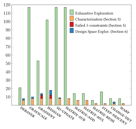
Figure 11. Number of invocations of the HLS tool for an exhaustive exploration (bars on the left) and COSMOS (on the right).

7.4. Summary

We report a brief summary of the achieved results:

• COSMOS guarantees a richer DSE with respect to the approaches that do not consider the memory as integral part of the DSE: for WAMI, COSMOS guarantees an average performance span of $4.06\times$ and an average area span of $2.58\times$ as opposed to $1.73\times$ and $1.22\times$, respectively, when only standard dual-port memories are used; COSMOS obtains a richer set of Pareto-optimal implementations thanks to memory generation and optimization;

• COSMOS guarantees a faster DSE compared to exhaustive search methods: for WAMI, COSMOS reduces the number of invocations to the HLS tool by $6.7\times$ on average and by up to $14.6\times$ for the single components; COSMOS is able to reduce the number of invocations thanks the compositional approach discussed in Section 6;

• COSMOS is an automatic and scalable methodology for DSE: the approach is intrinsically compositional, and thus with larger designs the performance gains are expected to be as good as smaller ones, if not better. While an exhaustive method has to explore all the alternatives, COSMOS focuses on the most critical components.

8. Related Work

This section describes the most-closely related methods to perform DSE. We distinguish the methods that explore single-component designs (reported in Section 8.1) from those that are compositional like COSMOS (in Section 8.2).

8.1. Component DSE

Several methods have been proposed to drive HLS tools for DSE. There exist probabilistic approaches (Schafer, 2016), search algorithms based on heuristics, such as simulated annealing (Schafer et al., 2009), iterative methodologies that exploit particle-swarm optimization (Mishra and Sengupta, 2014), as well as genetic algorithms (Ferrandi et al., 2008), and machine-learning-based exploration methodologies (Mahapatra and Schafer, 2014; Liu and Carloni, 2013; Schafer and Wakabayashi, 2012). All these methods try to quickly predict the relevance of the knobs and determine the Pareto curves of the scheduled RTL implementations in a multi-objective design space. None of these methods, however, consider the generation of optimized memory subsystems for hardware accelerators. Conversely, other methods focus on creating efficient memory subsystems, but without exploring the other HLS knobs. For instance, Pilato et al. (Pilato et al., 2014) propose a methodology to create optimized memory architectures, partially addressing the limitations of current HLS tools in handling memory subsystems. This enables a DSE that takes into account also the memory of accelerators. However, that work focuses on optimizing the memory architectures and not in proposing efficient DSE methods. Similarly, Cong et al. (Cong et al., 2016) explore memory reuse and non-uniform partitioning for minimizing the number of banks in multi-bank memory architectures for stencil computations. Differently from these works, COSMOS coordinates both memory generators, like the one proposed in (Pilato et al., 2017), and HLS tools to find several Pareto-optimal implementations of accelerators. Other methodologies apply both loop manipulations and memory optimizations. For instance, Cong et al. (Cong et al., 2012, 2011) adopt polyhedral-based analysis to apply loop transformations with the aim of optimizing memory reuse or partitioning. Differently from these works, COSMOS focuses on configuring the knobs provided by HLS, after applying such loop transformations. Indeed, COSMOS realizes a compositional-based methodology, and thus it finds Pareto-optimal implementations of the entire system, and not only of the single components. The first step of COSMOS consists in the characterization of components to identify regions of the multi-objective design space where feasible RTL implementations exist. This step differs from previous works (Schafer, 2016; Liu et al., 2011, 2012) for two main aspects. First, COSMOS includes memory generation and optimization in the DSE process. Second, COSMOS applies synthesis constraints to account for the high variability and partial unpredictability of the HLS tools. Such constraints consider both the dependency graph of the specification and the memory references in each loop. Thus, COSMOS identifies larger regions of Pareto-optimal implementations.

Other methods, such as Aladdin (Shao et al., 2014), perform a DSE without using HLS tools and without generating the RTL implementations, estimating the performance and costs of high-level specifications (C code for Aladdin). COSMOS differs from these methods because it aims at generating efficient RTL implementations by using HLS and memory generator tools. Indeed, such methods can be used before applying COSMOS to pre-characterize the different components of an accelerator that is not ready to be synthesized with HLS tools. Since the design of HLS-ready specifications requires significant efforts (Qamar et al., 2017), this can help the designers to focus only on the most critical components, i.e., those that are expected to return good performance gains over software executions. After this pre-characterization, COSMOS can be used to perform a DSE of such components and obtain the Pareto-optimal combinations of their RTL implementations.

8.2. System DSE

While the previous approaches obtain Pareto curves for single components, only few methodologies adopt compositional design methods for the synthesis of complex accelerators. The approach used by COSMOS predicts the Pareto curve at the system level, similarly to those proposed by Liu et al. (Liu et al., 2012) and Haubelt and Teich (Haubelt and Teich, 2003). Differently from these works, COSMOS correlates also the planned design points, which are simply theoretical (the LP solutions), with feasible high-level knob settings and memory configuration parameters. Further, COSMOS focuses on optimizing the HLS knobs, e.g., loop manipulations, and memory subsystems, rather than tuning low-level knobs, e.g., the target clock period.

9. Concluding Remarks

We presented COSMOS, an automatic methodology for compositional DSE that coordinates both HLS and memory generator tools. COSMOS takes into account the unpredictability of the current HLS tools and considers the PLMs of the components as an essential part of the DSE. The methodology of COSMOS is intrinsically compositional. First, it characterizes the components to define the regions of the design space that contain Pareto-optimal implementations. Then, it exploits a LP formulation to find the Pareto-optimal solutions at the system level. Finally, it identifies the knobs for each component that can be used to obtain the corresponding implementations at RTL. We showed the effectiveness and efficiency of COSMOS by considering the WAMI accelerator as a case study. Compared to methods that do not consider the PLMs, COSMOS finds a larger set of Pareto-optimal implementations. Additionally, compared to exhaustive search methods, COSMOS reduces the number of invocations to the HLS tool by up to one order of magnitude.

- (1)
- Amdahl (1967) M. Amdahl. 1967. Validity of the Single Processor Approach to Achieving Large Scale Computing Capabilities. In Proc. of the ACM Spring Joint Computer Conference (AFIPS).
- Baradaran and Diniz (2008) N. Baradaran and P. C. Diniz. 2008. A Compiler Approach to Managing Storage and Memory Bandwidth in Configurable Architectures. ACM Transaction on Design Automation of Electronic Systems (2008).
- Barker et al. (2013) K. Barker, T. Benson, D. Campbell, D. Ediger, R. Gioiosa, A. Hoisie, D. Kerbyson, J. Manzano, A. Marquez, L. Song, N. Tallent, and A. Tumeo. 2013. PERFECT (Power Efficiency Revolution For Embedded Computing Technologies) Benchmark Suite Manual. Pacific Northwest National Laboratory and Georgia Tech Research Institute. http://hpc.pnl.gov/PERFECT/.
- Borkar and Chien (2011) S. Borkar and A. Chien. 2011. The Future of Microprocessors. Communication of the ACM (2011).
- Boyd and Vandenberghe (2004) S. Boyd and L. Vandenberghe. 2004. Convex Optimization. Cambridge University Press.
- Campos et al. (1992) J. Campos, G. Chiola, J. M. Colom, and M. Silva. 1992. Properties and Performance Bounds for Timed Marked Graphs. IEEE Transactions on Circuits and Systems I: Fundamental Theory and Applications (1992).
- Carloni (2015) L. P. Carloni. 2015. From Latency-Insensitive Design to Communication-Based System-Level Design. Proc. of the IEEE (2015).
- Carloni (2016) L. P. Carloni. 2016. The Case for Embedded Scalable Platforms. In Proc. of the ACM/IEEE Design Automation Conference (DAC). (Invited).
- Chen et al. (2014) Y. Chen, T. Luo, S. Liu, S. Zhang, L. He, J. Wang, L. Li, T. Chen, Z. Xu, N. Sun, and O. Temam. 2014. DaDianNao: A Machine-Learning Supercomputer. In Proc. of the Annual ACM/IEEE International Symposium on Microarchitecture (MICRO).
- Chen et al. (2017) Y. H. Chen, T. Krishna, J. S. Emer, and V. Sze. 2017. Eyeriss: An Energy-Efficient Reconfigurable Accelerator for Deep Convolutional Neural Networks. IEEE Journal of Solid-State Circuits (2017).
- Cong et al. (2014) J. Cong, M. A. Ghodrat, M. Gill, B. Grigorian, K. Gururaj, and G. Reinman. 2014. Accelerator-Rich Architectures: Opportunities and Progresses. In Proc. of the ACM/IEEE Design Automation Conference (DAC).
- Cong et al. (2016) J. Cong, P. Li, B. Xiao, and P. Zhang. 2016. An Optimal Microarchitecture for Stencil Computation Acceleration Based on Nonuniform Partitioning of Data Reuse Buffers. IEEE Transactions on Computer-Aided Design of Integrated Circuits and Systems (2016).
- Cong et al. (2017) J. Cong, P. Wei, C. H. Yu, and P. Zhou. 2017. Bandwidth Optimization Through On-Chip Memory Restructuring for HLS. In Proc. of the Annual Design Automation Conference (DAC).
- Cong et al. (2011) J. Cong, P. Zhang, and Y. Zou. 2011. Combined Loop Transformation and Hierarchy Allocation for Data Reuse Optimization. In Proc. of the ACM/IEEE International Conference on Computer-Aided Design (ICCAD).
- Cong et al. (2012) J. Cong, P. Zhang, and Y. Zou. 2012. Optimizing Memory Hierarchy Allocation with Loop Transformations for High-Level Synthesis. In Proc. of the ACM/IEEE Design Automation Conference (DAC).
- Cota et al. (2015) E. G. Cota, P. Mantovani, G. Di Guglielmo, and L. P. Carloni. 2015. An Analysis of Accelerator Coupling in Heterogeneous Architectures. In Proc. of the ACM/IEEE Design Automation Conference (DAC).
- Ferrandi et al. (2008) F. Ferrandi, P. L. Lanzi, D. Loiacono, C. Pilato, and D. Sciuto. 2008. A Multi-objective Genetic Algorithm for Design Space Exploration in High-Level Synthesis. In Proc. of the IEEE Computer Society Annual Symposium on VLSI.
- Gerstlauer et al. (2009) A. Gerstlauer, C. Haubelt, A. D. Pimentel, T. P. Stefanov, D. D. Gajski, and J. Teich. 2009. Electronic System-level Synthesis Methodologies. IEEE Transactions on Computer-Aided Design of Integrated Circuits and Systems (2009).
- Ghenassia (2006) F. Ghenassia. 2006. Transaction-Level Modeling with SystemC. Springer-Verlag.
- Ham et al. (2016) T. J. Ham, L. Wu, N. Sundaram, N. Satish, and M. Martonosi. 2016. Graphicionado: A High-Performance and Energy-Efficient Accelerator for Graph Analytics. In Proc. of the Annual IEEE/ACM International Symposium on Microarchitecture (MICRO).
- Haubelt and Teich (2003) C. Haubelt and J. Teich. 2003. Accelerating Design Space Exploration Using Pareto-Front Arithmetics [SoC design]. In Proc. of the ACM/IEEE Asia and South Pacific Design Automation Conference (ASP-DAC).
- Horowitz (2014) M. Horowitz. 2014. Computing’s energy problem (and what we can do about it). In Proc. of the IEEE International Solid-State Circuits Conference (ISSCC).
- Kim (2017) L. W. Kim. 2017. DeepX: Deep Learning Accelerator for Restricted Boltzmann Machine Artificial Neural Networks. IEEE Transactions on Neural Networks and Learning Systems (2017).
- Kurra et al. (2007) S. Kurra, N. K. Singh, and P. R. Panda. 2007. The Impact of Loop Unrolling on Controller Delay in High Level Synthesis. In Proc. of the ACM/IEEE Conference on Design, Automation and Test in Europe (DATE).
- Li et al. (2011) B. Li, Z. Fang, and R. Iyer. 2011. Template-based Memory Access Engine for Accelerators in SoCs. In Proc. of the ACM/IEEE Asia and South Pacific Design Automation Conference (ASP-DAC).
- Liu and Carloni (2013) H. Y. Liu and L. P. Carloni. 2013. On Learning-Based Methods for Design-Space Exploration with High-Level Synthesis. In Proc. of the ACM/IEEE Design Automation Conference (DAC).
- Liu et al. (2011) H. Y. Liu, I. Diakonikolas, M. Petracca, and L. P. Carloni. 2011. Supervised Design Space Exploration by Compositional Approximation of Pareto Sets. In Proc. of the ACM/IEEE Design Automation Conference (DAC).
- Liu et al. (2012) H. Y. Liu, M. Petracca, and L. P. Carloni. 2012. Compositional System-Level Design Exploration with Planning of High-Level Synthesis. In Proc. of the AMC/IEEE Conference on Design, Automation, and Test in Europe (DATE).
- Liu et al. (2016) X. Liu, Y. Chen, T. Nguyen, S. Gurumani, K. Rupnow, and D. Chen. 2016. High Level Synthesis of Complex Applications: An H.264 Video Decoder. In Proc. of the ACM/SIGDA International Symposium on Field-Programmable Gate Arrays (FPGA).
- Lyons et al. (2012) M. J. Lyons, M. Hempstead, G. Y. Wei, and D. Brooks. 2012. The Accelerator Store: A Shared Memory Framework for Accelerator-based Systems. ACM Transactions on Architecture and Code Optimization (2012).
- Mahapatra and Schafer (2014) A. Mahapatra and B. Carrion Schafer. 2014. Machine-learning based Simulated Annealer Method for High Level Synthesis Design Space Exploration. In Proc. of the Electronic System Level Synthesis Conference (ESLsyn).
- Meeus et al. (2012) W. Meeus, K. Van Beeck, T. Goedemé, J. Meel, and D. Stroobandt. 2012. An Overview of Today’s High-Level Synthesis Tools. Design Automation for Embedded Systems (2012).
- Mishra and Sengupta (2014) V. K. Mishra and A. Sengupta. 2014. PSDSE: Particle Swarm Driven Design Space Exploration of Architecture and Unrolling Factors for Nested Loops in High Level Synthesis. In Proc. of the IEEE International Symposium on Electronic System Design (ISED).
- Murata (1989) T. Murata. 1989. Petri Nets: Properties, Analysis and Applications. Proc. of the IEEE (1989).
- Piccolboni et al. (2017) L. Piccolboni, P. Mantovani, G. Di Guglielmo, and L. P. Carloni. 2017. Broadening the Exploration of the Accelerator Design Space in Embedded Scalable Platforms. In Proc. of the IEEE High Performance Extreme Computing Conference (HPEC).
- Pilato et al. (2014) C. Pilato, P. Mantovani, G. Di Guglielmo, and L. P. Carloni. 2014. System-level Memory Optimization for High-level Synthesis of Component-based SoCs. In Proc. of the ACM/IEEE International Conference on Hardware/Software Codesign and System Synthesis (CODES+ISSS).
- Pilato et al. (2017) C. Pilato, P. Mantovani, G. Di Guglielmo, and L. P. Carloni. 2017. System-Level Optimization of Accelerator Local Memory for Heterogeneous Systems-on-Chip. IEEE Transactions on Computer-Aided Design of Integrated Circuits and Systems (2017).
- Porter et al. (2010) R. Porter, A. M. Fraser, and D. Hush. 2010. Wide-Area Motion Imagery. IEEE Signal Processing Magazine (2010).
- Qamar et al. (2017) A. Qamar, F. B. Muslim, F. Gregoretti, L. Lavagno, and M. T. Lazarescu. 2017. High-Level Synthesis for Semi-Global Matching: Is the Juice Worth the Squeeze? IEEE Access (2017).
- Ramamoorthy and Ho (1980) C. V. Ramamoorthy and G. S. Ho. 1980. Performance Evaluation of Asynchronous Concurrent Systems Using Petri Nets. IEEE Transaction on Software Engineering (1980).
- Reagen et al. (2016) B. Reagen, P. Whatmough, R. Adolf, S. Rama, H. Lee, S. K. Lee, J. M. Hernández-Lobato, G. Y. Wei, and D. Brooks. 2016. Minerva: Enabling Low-Power, Highly-Accurate Deep Neural Network Accelerators. In Proc. of the ACM/IEEE Annual International Symposium on Computer Architecture (ISCA).
- Sangiovanni-Vincentelli (2007) A. Sangiovanni-Vincentelli. 2007. Quo Vadis, SLD? Reasoning About the Trends and Challenges of System Level Design. Proc. of the IEEE (2007).
- Schafer (2016) B. Carrion Schafer. 2016. Probabilistic Multiknob High-Level Synthesis Design Space Exploration Acceleration. IEEE Transactions on Computer-Aided Design of Integrated Circuits and Systems (2016).
- Schafer et al. (2009) B. Carrion Schafer, T. Takenaka, and K. Wakabayashi. 2009. Adaptive Simulated Annealer for High Level Synthesis Design Space Exploration. In Proc. of the IEEE International Symposium on VLSI Design, Automation and Test (VLSI-DAT).
- Schafer and Wakabayashi (2012) B. Carrion Schafer and K. Wakabayashi. 2012. Machine Learning Predictive Modelling High-Level Synthesis Design Space Exploration. IET Computers Digital Techniques (2012).
- Seznec (2015) A. Seznec. 2015. Bank-interleaved Cache or Memory Indexing Does Not Require Euclidean Division. In Proc. of the Annual Workshop on Duplicating, Deconstructing, and Debunking (WDDD).
- Shao et al. (2014) Y. S. Shao, B. Reagen, G. Y. Wei, and D. Brooks. 2014. Aladdin: A Pre-RTL, Power-performance Accelerator Simulator Enabling Large Design Space Exploration of Customized Architectures. In Proc. of the ACM/IEEE Annual International Symposium on Computer Architecture (ISCA).
- Zhang et al. (2015) C. Zhang, P. Li, G. Sun, Y. Guan, B. Xiao, and J. Cong. 2015. Optimizing FPGA-based Accelerator Design for Deep Convolutional Neural Networks. In Proc. of the ACM/SIGDA International Symposium on Field-Programmable Gate Arrays (FPGA).