Piercing the rainbow: entanglement on an inhomogeneous spin chain with a defect

Abstract

The rainbow state denotes a set of valence bond states organized concentrically around the center of a spin 1/2 chain. It is the ground state of an inhomogeneous XX Hamiltonian and presents maximal violation of the area law of entanglement entropy. Here, we add a tunable exchange coupling constant at the center, $\gamma$, and show that it induces entanglement transitions of the ground state. At very strong inhomogeneity, the rainbow state survives for $0\leq\gamma\leq 1$, while outside that region the ground state is a product of dimers. In the weak inhomogeneity regime the entanglement entropy satisfies a volume law, derived from CFT in curved spacetime, with an effective central charge that depends on the inhomogeneity parameter and $\gamma$. In all regimes we have found that the entanglement properties are invariant under the transformation $\gamma\longleftrightarrow 1-\gamma$, whose fixed point $\gamma=\frac{1}{2}$ corresponds to the usual rainbow model. Finally, we study the robustness of non trivial topological phases in the presence of the defect.

I Introduction

Entanglement provides a very useful connecting thread through condensed matter physics, quantum optics and quantum field theory, towards a unified field of quantum matter Amico.08 ; Laflorencie.16 . One of the most relevant insights is expressed through the area law Hastings2006 ; Wolf2008 : the entanglement entropy of a block within the ground state (GS) of a local quantum system is, in general terms, proportional to the measure of its boundary Sredniki.93 ; Eisert.10 . Interestingly, the GS of a (1+1)D conformal field is an exception, and the entropy of a block is generically proportional to the logarithm of its volume, with a prefactor which is proportional to the associated central charge Holzhey.94 ; Vidal.03 ; Calabrese.04 ; Calabrese.09 . There are other interesting exceptions, such as random systems Refael.04 ; Refael.04b ; Laflorencie.05 ; Fagotti.11 ; Ramirez.14 ; Ruggiero.16 . In the strong inhomogeneity limit, the GS of many random systems can be obtained via the Dasgupta-Ma procedure Dasgupta.80 ; Fisher.95 , which can be engineered to obtain a 1D GS with maximal entanglement between its left and right halves, known as the rainbow state Vitagliano.10 ; Ramirez.14b ; Ramirez.15 ; Samos.19 . This violation of the area law is very robust with respect to the presence of disorder in the hoppings Laguna.16 ; Alba.19 .

A physical interpretation of the rainbow state can be provided by noticing that the Dirac vacuum on a static (1+1)D metric of optical type can be simulated on a free fermionic lattice with smoothly varying hopping amplitudes Boada.11 ; Laguna.17 . Indeed, the hopping amplitudes which characterize the rainbow state can be understood as a (1+1)D anti-de Sitter (AdS) metric Laguna.17b ; Tonni.18 ; MacCormack.18 . Space is exponentially stretched as we move away from the center, giving rise to a similar exponential stretch of the entanglement entropies, transforming the logarithmic law into a volume law. The weak inhomogeneity limit is determined by a deformation of the conformal law and the strong inhomogeneity limit is determined by the Dasgupta-Ma rule, and both fit seamlessly.

Thus, it is relevant to ask whether the weak and the strong inhomogeneity limits will match in all possible situations. We have introduced a defect in the center of the rainbow system and considered the entanglement structure as a function of the defect intensity and the curvature. As we will show, both the Dasgupta-Ma and the field theory approach that describes entanglement on a critical chain with a defect Levine.04 ; Peschel.05 ; Igloi.09 ; Eisler.10 can be extended to the curved case in the strong and weak inhomogeneity regimes, respectively, providing a complete physical picture.

This article is organized as follows. Section II discusses our model. The strong inhomogeneity limit, studied with the Dasgupta-Ma RG, is described in detail in Sec. III, while Sec. IV considers the weak-inhomogeneity regime through a perturbation of a conformal field theory. We characterize the entanglement structure via the entropies and the entanglement spectrum, Hamiltonian and contour. A duplication of the defect leads the system to a symmetry protected topological (SPT) phase in coexistence with a trivial dimerized phase, which are discussed in Sec. V. The article ends with a brief discussion of our conclusions and proposals for further work in Sec. VI.

II The model

Let us consider a fermionic open 1D free fermion system with an even number of sites $N=2L$ whose Hamiltonian is defined as:

$$H_{L}(h,\gamma)=-\frac{1}{2}\sum_{m=-L+1}^{L-1}J_{m}c^{\dagger}_{m-1/2}c_{m+1/2}+\text{h.c.},$$ (1)

where $c_{n}(c^{\dagger}_{n})$, with $n=\pm\frac{1}{2},\pm\frac{3}{2}\dots\pm(L-\frac{1}{2})$ are fermionic annihilation (creation) operators that obey the standard anti-commutation relations. The hopping parameters $J_{m}$ are

$$J_{m}=\begin{cases}e^{-h|m|}&\text{if }m\neq 0,\\ e^{-h\gamma}&m=0,\\ \end{cases}$$ (2)

where $h\geq 0$ is the inhomogeneity parameter, and $\gamma\in{\mathbb{R}}$ parametrizes the value of the central hopping that we shall interpret as a defect. Notice that sites have half-integer indices, while links have integer ones. The Hamiltonian presents spatial inversion symmetry around the central bond: $J_{m}=J_{-m}$, which we will label bond-centered symmetry (bcs) Samos.19 .

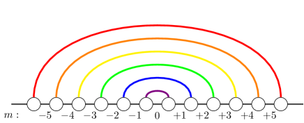
Figure 1: Illustrating the rainbow state, GS of $H_{L}(h,1/2)$ with $L=6$, for $h\gg 1$. Links are indexed by the integer $m$. The bonds are established between sites $n$ and $-n$ for $n\in\{\pm 1/2,\cdots,\pm L/2-1\}$.

For $\gamma=1/2$ we recover the so-called rainbow Hamiltonian, whose ground state is the rainbow state Vitagliano.10 ; Ramirez.14b ; Ramirez.15 . In the strong-coupling regime ($h\gg 1$), the GS of $H_{L}(h,1/2)$ is a valence bond solid (VBS) made of bonds connecting opposite sites of the chain, as is illustrated in Fig. 1. On the other hand, the weak coupling limit ($h\ll 1$) is characterized by the free-fermion conformal field theory (CFT) on a different space-time, provided by the metric

$$ds^{2}=-e^{-2h|x|}dt^{2}+dx^{2},$$ (3)

thus justifying our claim that the rainbow state, in the weak coupling regime, corresponds to the anti de Sitter (AdS) Dirac vacuum. Using CFT tools, it has been proved that the GS of Hamiltonian $H_{L}(h,1/2)$ presents linear entanglement for all $h$, with an entropy per site $S/N\approx h/6$ (von Neumann entanglement entropy) Laguna.17b ; Tonni.18 . We will discuss some of these properties in detail in the corresponding sections, when considering how they are modified by the defect.

III The strong inhomogeneity limit

When the inhomogeneity is large enough, it can be addressed through renormalization group (RG) schemes. In particular we will use the Dasgupta-Ma procedure, also known as strong-disorder renormalization group (SDRG) Dasgupta.80 , that was originally created to characterize random spin chains, but can be immediately extended to fermionic chains via de Jordan-Wigner transformation Ramirez.14 . At each step of the RG, four spins are considered: the two spins ($s_{i}$ and $s_{i+1}$ linked by the strongest coupling (highest absolute value of $J_{i}$) and their nearest neighbours, $s_{i-1}$ and $s_{i+2}$. The two spins coupled by $J_{i}$ are integrated out by forming a valence bond state (VBS) and the two remaining ones are coupled with a new effective coupling constant that is obtained by means of second order perturbation theory. For a free-fermionic chain with a Hamiltonian such as (1), the effective coupling takes the expression

$$\tilde{J}_{i}=-{J_{i-1}J_{i+1}\over J_{i}},\qquad|J_{i}|\gg|J_{i\pm 1}|.$$ (4)

The GS predicted by the SDRG is a valence-bond solid (VBS) i.e. a tensor product of bonds:

$$\ket{GS}=\prod_{k=1}^{L}(b^{\eta_{k}}_{i_{k},j_{k}})^{\dagger}\ket{0},$$ (5)

where $\eta_{k}=\pm 1$ is a phase given by Eq. (4), $\ket{0}$ is the Fock vacuum and $b^{+}_{i,j}$ ($b^{-}_{i,j}$) are bonding (anti-bonding) operators that create a fermionic excitation joining sites $i$ and $j$.

$$\left(b^{\pm}_{ij}\right)^{\dagger}=\frac{1}{\sqrt{2}}\left(c^{\dagger}_{i}\pm c^{\dagger}_{j}\right).$$ (6)

They satisfy usual canonical anti-commutation relations. For our purposes, it is convenient to define the log-couplings Laguna.16 ,

$$t_{i}=-\log\frac{|J_{i}|}{h},$$ (7)

where $h$ is the inhomogeneity parameter that is included for later convenience. In this language, the two fermionic sites that are integrated out are those connected by the lowest $t_{i}$ and the effective coupling Eq. (4) is computed in additive way:

$$\tilde{t}_{i}=t_{i-1}-t_{i}+t_{i+1}.$$ (8)

Interestingly, Eq. (8) can be generalized for this type of models: whenever a bond is established between sites $p$ and $q$ (with $p+q$ even), the renormalized log-coupling is given by the sum rule Alba.19 :

$$\tilde{t}_{[p,q]}=\sum_{j=0}^{q-p-1}(-1)^{j}t_{p+j},$$ (9)

or, in other words: the renormalized log-coupling can be obtained summing all log-coupling between the two extremes, with alternating signs.

Let us consider the GS of Hamiltonian (1) under the light of the SDRG for $h\gg 1$. For simplicity, we will only consider even $L$ (the case of odd $L$ can be straightforwardly obtained), as a function of the defect parameter, $\gamma$. The different phases will be discussed along the panels of Fig. 2. In Fig. 2 (a) we have plotted the values of the log-couplings, for later reference: $\{\cdots,2,1,\gamma,1,2,\cdots\}$.

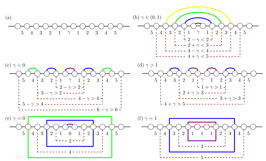
Figure 2: (a) Illustration of the rainbow chain with a central defect, showing the log-couplings on each link; (b) SDRG procedure in the $\gamma\in(0,1)$ case, leading to the rainbow phase; (c) SDRG for the $\gamma<0$ case; (d) SDRG for the $\gamma>1$ case, both leading to dimerized phases; (e) and (f) transition cases, where the SDRG approximation is not valid; the dashed boxes mark the ties between the couplings, which demand a different RG approach.

• The rainbow phase: $\gamma\in(0,1)$, see Fig. 2 (b). The strongest link (lowest log-coupling) is the central one. Thus, a valence bond is established on top ($b^{+}_{-1/2,+1/2}$) and an effective log-coupling appears between its neighbors, of magnitude $\tilde{t}=2-\gamma<2$. Thus, the central link is again the strongest one, so we can put a valence-bond on top of it ($b^{-}_{-3/2,+3/2}$), leading to an effective log-coupling of magnitude $\tilde{t}=2+\gamma<3$. We can see that the procedure iterates, giving rise to the rainbow state.

  $$\ket{GS}_{\gamma\in(0,1)}=\prod_{i=0}^{L-1}\left(b^{\eta_{i}}_{-i-1/2,i+1/2}\right)^{\dagger}\ket{0},\quad\eta_{i}=(-1)^{i}.$$ (10)

• The dimerized phase (I): $\gamma<0$, see Fig. 2 (c). The dominant interaction is again the central one, leading us to establish a valence bond on top. Yet, the renormalized log-coupling, $\tilde{t}=2-\gamma>2$ is not the strongest (lowest value) at the next SDRG iteration. On the other hand, we are led to establish two valence bonds on top of the links with log-couplings equal to 2, in any order. The renormalized central log-coupling after these two bonds have been established is $\tilde{t}=4-\gamma>4$ (see Eq. (9)), so we are led to the same situation, where the lateral links are always stronger than the central one, leading to a dimerized state. Yet, the last SDRG step leaves us with the two extreme sites of the chain, leading to a final bond connecting them. The ground state can be written as

  $$\ket{GS}_{\gamma<0}=(b^{-}_{-L+\frac{1}{2},L-\frac{1}{2}})^{\dagger}\prod_{i=-\frac{L}{2}+1}^{\frac{L}{2}-1}(b^{+}_{2i-\frac{1}{2},2i+\frac{1}{2}})^{\dagger}\ket{0}.$$ (11)

  Notice that the last bond is only present for even $L$, while it is absent for odd $L$.

• The dimerized phase (II): $\gamma>1$, see Fig. 2 (d). In this case, the dominant interaction is not the central one, but their neighbors, with $t_{\pm 1}=1$. Hence, we must establish first these two valence bonds, leading to a renormalized log-coupling between their extremes of $\tilde{t}=2+\gamma>3$ (see Eq. (9)). Thus, we have the same situation, in which the central link is not the strongest. In this case, no long-range bond is established at the end of the procedure, and we obtain

  $$\ket{GS}_{\gamma>1}=\prod_{i=-\frac{L-1}{2}}^{\frac{L-1}{2}}(b^{+}_{2i-\frac{1}{2},2i+\frac{1}{2}})^{\dagger}\ket{0}.$$ (12)

  Both dimerized phases are related to the two phases of the Su-Schrieffer-Heeger (SSH) model Su.79 ; Heeger.88 .

• The transition points: $\gamma=1$ and $\gamma=0$, see Fig. 2 (e) and (f). Let us start with $\gamma=1$ (Fig. 2 (e)). The first SDRG step fails, because the strongest coupling is not unique. On the other hand, we obtain a triple tie in the three central links, with $t_{0,\pm 1}=1$. In Appendix A we have developed an extension of the SDRG for the free-fermion model when a block with $2\ell$ sites is integrated out, yielding the renormalized log-coupling given by the sum rule, Eq. (9). Thus, the renormalized log-coupling between sites $-5/2$ and $+5/2$ is $\tilde{t}=3$, leading to a new triple tie, which propagates further along the chain. For $\gamma=0$, on the other hand, the strongest link is the central one, thus receiving a valence bond. But, on the next SDRG step, we can see that the effective central log-coupling is $\tilde{t}=2$, equal to its neighbors in a new triple tie, forcing us to recourse to the extended SDRG. From that moment on, all SDRG steps lead to triple ties. The GS can be written exactly in these two cases (see details in Appendix B)

  $$\ket{GS}_{\gamma=0}=(b^{-}_{-L+\frac{1}{2},L-\frac{1}{2}})^{\dagger}\prod_{i=1}^{\frac{L}{4}}(d^{\eta_{i}}_{2i+\frac{1}{2}})^{\dagger}(b^{+}_{-\frac{1}{2},\frac{1}{2}})^{\dagger}\ket{0},$$ (13)

  $$\ket{GS}_{\gamma=1}=\prod_{i=1}^{\frac{L}{2}}(d^{\eta_{i}}_{2i-\frac{1}{2}})^{\dagger}\ket{0},$$ (14)

  where $d^{\pm}_{k}$ is operators creating two particles on four fermionic sites,

  $$(d^{\eta_{i}}_{i})^{\dagger}=(v^{\eta_{i}})^{\dagger}(u^{\eta_{i-1}})^{\dagger}\ket{0},\quad\eta_{i}=(-1)^{i},$$ (15)

  $$u^{\pm}_{i}=\frac{1}{\sqrt{5+\sqrt{5}}}(c_{-i}\pm c_{i})+\frac{1}{\sqrt{5-\sqrt{5}}}(c_{-i+1}\pm c_{i-1}),$$ (16)

  $$v^{\pm}_{i}=\frac{1}{\sqrt{5-\sqrt{5}}}(c_{-i}\pm c_{i})+\frac{1}{\sqrt{5+\sqrt{5}}}(c_{-i+1}\pm c_{i-1}).$$ (17)

The aforementioned description, along with the evidences presented in the rest of this section allow us to claim that the rainbow system with a defect presents two entanglement transitions Vasseur2018 in the strong inhomogeneity regime.

It is worth to notice the existence of a symmetry between the cases $\gamma\leq 0$ and $\gamma\geq 1$. Consider a system $H_{L}(h,\gamma<1)$. After performing the first RG step, the new system is described by the renormalized Hamiltonian $H_{L-1}(h,2-\gamma)$. If we now subtract one from all the log-hoppings (or equivantly we divide by $e^{-h}$ all the hoppings) the Hamiltonian becomes $e^{h}H_{L-1}(h,1-\gamma)$, which describes a system of $N-2$ sites and a defect with strength $1-\gamma$. Hence, the transformation

$$\gamma\to\tilde{\gamma}=1-\gamma,$$ (18)

leaves the structure invariant (up to a global constant). Note that this symmetry can be considered as a local strong-weak duality of the defects, leaving the $\gamma=1/2$ point invariant.

The structure of the different phases of the rainbow system with a defect can be properly understood if we fold the chain around the central link, as it is shown in Fig. 3 (a), converting the chain into a two-rung ladder where sites $+k$ and $-k$ face each other Samos.19 . This transformation converts rainbow bonds into vertical bonds and the remaining local bonds into horizontal bonds. The lower panels of Fig. 3 present the bond structure as a function of $\gamma$.

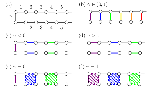
Figure 3: (a) Folding the rainbow into a two-rung ladder; (b) folded rainbow structure, obtained for $\gamma\in(0,1)$; (c) and (d) folded dimerized structures, for $\gamma<0$ and $\gamma>1$; (e) and (f) folded versions of the transition points, with the plaquettes marked where operators $d^{\dagger}$ act, see Eq. (15).

III.1 Energies

Let us consider the single-body energy levels $E_{k}(h,\gamma)$ ($k\in\{0,\cdots,N-1\}$) of $H_{L}(h,\gamma)$, , obtained by diagonalizing the corresponding hopping matrix. Due to the particle-hole symmetry, $E_{k}=-E_{N-k}$, we need only consider values up to $L-1$. For large $h$, these single-body energy levels correspond to the couplings associated with each valence bond, thus leading us to propose that the following limits are finite,

$$\lim_{h\to\infty}-{\log|E_{k}(h,\gamma)|\over h}=\Xi_{k}(\gamma).$$ (19)

Fig. 4 (top) plots these values, $\Xi_{k}(\gamma)$ as a function of $\gamma$ for $L=12$, obtained numerically using $h=15$ (for which convergence has been achieved and ). Notice the clear pattern: for $\gamma>1$, all energy levels are degenerate, $\Xi_{2k}(\gamma)=\Xi_{2k+1}(\gamma)=2k+1$ for $k\in\{0,\cdots,L/2-1\}$, while for $\gamma<0$ all energy levels are degenerate and constant, except the first and last which vary exponentially with $\gamma$, $\Xi_{2k-1}(\gamma)=\Xi_{2k}(\gamma)=2k$ for $k\in\{1,\cdots,L/2-1\}$. Indeed, these values correspond to the energies associated to the successive valence bonds of the dimerized phases. On the other hand, for $\gamma\in(0,1)$ the energy levels are not degenerate, and we can observe the same alternation of the renormalized log-couplings that we observed in the SDRG description: $\Xi_{k}(\gamma)=k+1/2+(-1)^{k}(\gamma-1/2)$. Thus, the transition points, $\gamma=0$ and $\gamma=1$, correspond to the points where the degeneracy starts and ends.

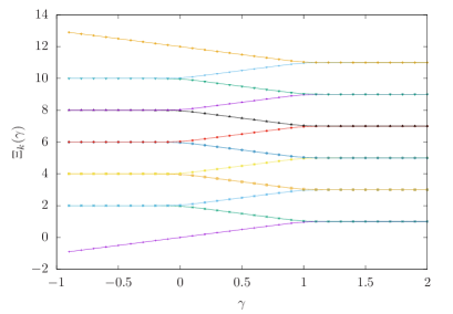
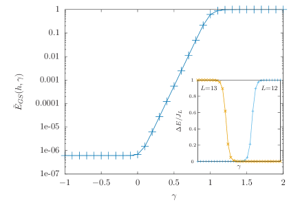
Figure 4: Top: plot of $\Xi_{k}(\gamma)$, obtained numerically for $L=12$ and $h=15$, see Eq. (19). Each curve matches the renormalized log-couplings along the SDRG procedure. Bottom: ground state energy, with the lowest single-body energy level removed, as a function of $\gamma$ for the same system. Inset: energy gap in units of the lowest energy scale of the system, $\Delta E/J_{L}$, for $L=12$ and $L=13$.

The ground state energy is the sum of the energies of the occupied orbitals, $E_{GS}(h,\gamma)=\sum_{k=0}^{L-1}E_{k}(h,\gamma)$. Notice that for large $h$ and $\gamma>1$, the lowest single-body energy $E_{0}(h,\gamma)$ is the main contribution to $E_{GS}(h,\gamma)$ as its value grows exponentially with $\gamma$ (see the lowest line of the top panel of Fig. 4), so we have considered instead the quantity

$$\tilde{E}_{GS}(h,\gamma)=-E_{GS}(h,\gamma)+E_{0}(h,\gamma)=-\sum_{k=1}^{L-1}E_{k}(h,\gamma).$$ (20)

The values of $\tilde{E}_{GS}(h,\gamma)$ are plotted in Fig. 4 (bottom) for the same system $L=12$ and $h=15$, in logarithmic scale. Notice the three regions: for the dimerized phases, $\tilde{E}_{GS}(h,\gamma)$ stays constant, while for the rainbow phase it grows exponentially. Indeed, for $h\to\infty$, the energy curve $\log(\tilde{E}_{GS}(h,\gamma))/h$ becomes non-smooth at $\gamma=0$ and $\gamma=1$, pointing at a phase transition.

In addition, the inset of Fig. 4 (bottom) plots the energy gap $\Delta E/J_{L}=\left(E_{L}-E_{L-1}\right)/J_{L}$, normalized with the lowest energy scale of the system (the lowest coupling constant). We can see that it presents two types of behaviors, depending wether the spectrum has a long range mode (with $E_{L-1}(h,\gamma)=e^{-Lh}$): for even $L$ it is close to zero ($\Delta E/J_{L}\sim e^{-h}$) for $\gamma<1$, while for odd $L$ it is close to zero ($\Delta E/J_{L}\sim e^{-h}$) for $\gamma>0$. For $\gamma\in[0,1]$, it is close to zero for all sizes.

III.2 Correlations and order parameters

In order to provide further support to our idea that there is a phase transition at $\gamma=0$ and $\gamma=1$ in the strong coupling limit, let us provide two order parameters, that we will call the dimerization parameter, $\Delta_{d}$ and the rainbow parameter, $\Delta_{r}$,

$$\Delta_{d} = \frac{1}{N}\sum_{i=-L+\frac{1}{2}}^{L-\frac{1}{2}}|\langle\psi|c^{\dagger}_{i}c_{i+1}|\psi\rangle|$$ (21)

$$\Delta_{r} = \frac{1}{L}\sum_{i=-\frac{1}{2}}^{L-\frac{1}{2}}|\langle\psi|c_{i}^{\dagger}c_{-i}|\psi\rangle|.$$ (22)

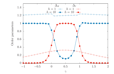
Figure 5: Dimerization parameter $\Delta_{d}$ (blue curves) and rainbow parameter $\Delta_{r}$ (red curves) as a function of $\gamma$, for a system of $L=10$. As the inhomogeneity parameter $h$ grows, $\Delta_{d}$ approaches one in the dimerized phases and zero in the rainbow phase, while $\Delta_{r}$ approaches one in the rainbow phase and zero in the dimerized phases.

Fig. 5 shows the behavior of these two order parameters as a function of $\gamma$, for two values of $h$ and $L=10$. For large $h$ ($h=10$ in the figure), we see that the rainbow parameter $\Delta_{r}$ tends to 1 in the rainbow phase ($\gamma\in(0,1)$), while it decays to zero in the dimerized phases. The opposite behavior is true for the dimerization parameter $\Delta_{d}$.

III.3 Entanglement entropy

Given a system in a pure state, $\ket{\psi}$, the entanglement entropy (EE) of a block $A$ is defined as the von Neumann entropy of its associated reduced density matrix $\rho_{A}=\Tr_{\bar{A}}\ket{\psi}\bra{\psi}$, where $\bar{A}$ is the complementary of $A$.

$$S[\rho_{A}]=-\Tr\rho_{A}\log(\rho_{A}),$$ (23)

while the Rényi entropy of order $n$ is defined as

$$S^{(n)}[\rho_{A}]=\frac{1}{1-n}\log\Tr\rho_{A}^{n}.$$ (24)

Needless to say, the different entanglement entropies are determined by the eigenvalues of the reduced density matrix, also known as entanglement spectrum (ES). There is well known procedure Peschel.03 in order to obtain the ES through the spectrum of the correlation matrix restricted to the block, $\langle c^{\dagger}_{i}c_{j}\rangle$, with $i$, $j\in A$. The correlation matrices can be exactly obtained in the strong coupling limit, as it is shown in Appendix C. On the other hand, when the state is a VBS, we can evaluate the EE just by counting the number of bonds which are broken when we detach the block from its environment, and multiplying by $\log(2)$, and the same is true for all Rényi entropies.

We have considered two different types of blocks: lateral blocks start from the extreme of the chain, while central blocks are symmetric with respect to the center. In the next paragraphs we will describe the behavior of their entanglement.

III.3.1 Lateral blocks. Half chain entropies

Lateral blocks $A_{\ell}=\{-L+\frac{1}{2},\dots,-L+\frac{1}{2}+\ell\}$ are contiguous blocks containing one of the extremes of the chain. Concretely, we will be interested in the EE of the half chain, $S(L)=S[A_{L}]$ in the strong coupling regime for different values of $\gamma$. Let us remind the reader that we will only consider even $L$ for simplicity, and that the different phases can be visualized either in Fig. 2 and Fig. 3, where the blocks contain $\ell$ sites from the upper leg, starting from the right end.

• Rainbow phase, $\gamma\in(0,1)$: the EE (and all other Rényi entropies) are merely proportional to the lenght up to $\ell=L$, $S[A_{\ell}]_{\gamma\in(0,1)}=\log(2)\min(\ell,2L+1-\ell)\,$.

• Dimerized phases, $\gamma<0$ or $\gamma>1$: the lateral blocks cut either zero or one bonds for $\gamma>1$, $S[A_{\ell}]_{\gamma>1}=\log(2)(1-(-1)^{\ell})/2$; yet, for $\gamma<0$ there is always a long-distance bond joining both ends, thus $S[A_{\ell}]_{\gamma<0}=\log(2)\left(1+(1+(-1)^{\ell})/2\right)$.

• Transition cases: $\gamma=0$ and $\gamma=1$: The state is not a VBS, so the EE of a block can not be evaluated just by counting broken bonds. As we can see in the folded view, Fig. 3, the sites are grouped into plaquettes (except, maybe, for the extremes and the central link). Cutting one of these plaquettes horizontally in half contributes a finite amount of entanglement $S_{a}$, which is exactly evaluated in Appendix C (see Eq. (15)):

  $$S_{a}=\log 20-\frac{4\tanh^{-1}\left(\frac{2}{\sqrt{5}}\right)}{\sqrt{5}}\approx 0.4133,$$ (25)

  we are thus led to exact expressions for the half-chain entropy: $S[A_{L}]_{\gamma=1}=S_{a}\,L/2\log(2)$, $S[A_{L}]_{\gamma=0}=S_{a}\,(L/2-1)+2\log(2)$.

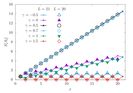
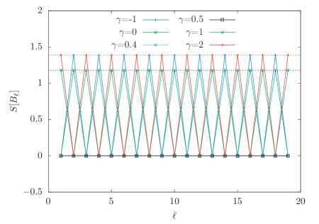
Figure 6: Top: Entanglement entropy of blocks of size $\ell$ using $h=10$ for two systems, of size $L=20$ and $L=21$, for different values of $\gamma$. Bottom: EE of the central blocks $B_{\ell}$ for $L=20$ sites and $h=10$. The top horizontal line marks $2\log 2$, and the lower one marks $S_{b}$, see Eq. (26)

.

All these results can be checked in Fig. 6 (top) for two rainbow chains with $L=20$ and $L=21$, using $h=10$, where $S[A_{\ell}]$ is plotted as a function of $\ell$ for different values of $\gamma$. We can see that the $\gamma=-0.5$ and $\gamma=1.5$ cases show a properly dimerized behavior, and the $\gamma=0.5$ values correspond to the rainbow, linear with (maximal) slope $\log(2)$. For the transition points, $\gamma=0$ and $\gamma=1$ we can observe a linear behavior (with parity oscillations) with a slope $S_{a}$.

III.3.2 Central blocks

In this subsection we consider the EE of central blocks, symmetrically placed around the center of the chain, $B_{\ell}=\{-\ell+\frac{1}{2},\cdots,\ell-\frac{1}{2}\}$. Again, we suggest the reader to refer to the corresponding panels of Fig. 2 and Fig. 3, where the blocks now include $\ell$ rungs starting from the left extreme.

• Rainbow phase, $\gamma\in(0,1)$: we always have $S[B_{\ell}]_{\gamma\in(0,1)}=0$.

• Dimerized phases, $\gamma<0$ or $\gamma>1$: central blocks either cut zero or two bonds. Always usign even $L$ we have $S[B_{\ell}]_{\gamma<0}=(1+(-1)^{\ell})\log(2)$ and $S[B_{\ell}]_{\gamma>1}=(1-(-1)^{\ell})\log(2)$.

• Transition phases, $\gamma=0$ or $\gamma=1$: central blocks can cut plaquettes in half vertically, in the folded view. Each such cut contributes a finite amount of entanglement, given by (See Appendix C and Eq. (15)):

  $$S_{b}=\log 5-\frac{\coth^{-1}\left(\sqrt{5}\right)}{\sqrt{5}}\approx 1.1790,$$ (26)

  which leads us to the expressions $S[B_{\ell}]_{\gamma=0}=(1+(-1)^{\ell})S_{b}$ and $S[B_{\ell}]_{\gamma=1}=(1-(-1)^{\ell})S_{b}$.

All these features can be checked in Fig. 6 (bottom), where we can see the central blocks entropy $S[B_{\ell}]$ as a function of $\ell$ for different values of $\gamma$. Note that the EE of the central blocks is always bounded, thus obeying the area law. Non-local fermionic excitations of the type $b_{i,-i}$ and $d_{i}$ (see Eq. (6) and Eq. (15)) are made local by the folding operation previously discussed Samos.19 , and allows to describe the system state using only short range entanglement (SRE).

It is important to realize that it is possible to find local blocks whose EE is zero independently of the defect (see Fig. 3). This means that the system is topologically trivial for all $\gamma$ Samos.19 . On section V we will discuss the site centered symmetry case, that presents interesting topological features.

IV Weak inhomogeneity: defect on a deformed background

It is relevant to ask whether the phases described in the strong inhomogeneity limit and the corresponding entanglement transitions extend into the weak inhomogeneity regime. The answer is no, but some relevant traits do.

In Fig 7 we show the dependence on $h$ of the EE of the half chain, $S(L)=S[A_{L}]$, for different values of $\gamma$. We can observe a perfect symmetry between $\gamma$ and $1-\gamma$, and the three different trends in the large $h$ limit that we have explained on the previous section: for $\gamma\in(0,1)$ the EE reaches its maximal value; for $\gamma\in\{0,1\}$, it reaches an intermediate value ($S_{a}L/2$); for $\gamma\not\in[0,1]$, it stays at $\log(2)$. Interestingly, the behaviour is remarkably different for lower values of $h$, as we will discuss.

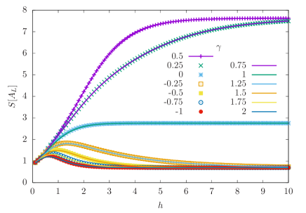
Figure 7: EE of the half system $N=22$ as a function of $h$ for different values of the defect strength $\gamma$.

For $h=0$ the Hamiltonian (1) becomes the standard massless free-fermionic chain with open boundary conditions (OBC) which can be described at low energies by a conformal field theory (CFT) with $c=1$. It is interesting to discuss first such a system in presence of a defect.

IV.1 Homogeneous chain with defect

Let us consider an homogeneous free fermionic chain with OBC and a defect on its central link, parametrized by a coupling parameter $\tau$,

$$H_{\tau}=-\frac{\tau}{2}c_{-\frac{1}{2}}^{\dagger}c_{\frac{1}{2}}-\frac{1}{2}\sum_{n=1/2}^{L-3/2}c^{\dagger}_{n}c_{n+1}+c^{\dagger}_{-n}c_{-n-1}+\text{h.c.}$$ (27)

Let us take the continuum limit of (27) and characterize its low-energy properties by expanding the local operators $c_{n}$ into slow left/right moving components $\psi_{\{L,R\}}$ around the Fermi points, and introducing a physical coordinate $x=an$, with lattice constant $a\to 0$, while $L\to\infty$ with $\mathcal{L}=aL$ fixed.

$$c_{m}\approx\sqrt{a}\left(e^{ik_{F}x}\psi_{L}(x)+e^{-ik_{F}x}\psi_{R}(x)\right).$$ (28)

The boundary conditions satisfied by the fields at the edge boundaries $\psi_{L,R}(\pm\mathcal{L})$ are obtained by imposing $c_{\pm(L+\frac{1}{2})}=0$:

$$\psi_{L}(\mathcal{\pm L})=e^{i\pi(L\pm\frac{1}{2})}\psi_{R}(\mathcal{\pm L}).$$ (29)

In order to characterize the effect of the defect $\tau$, we need to distinguish between the fields on the left side $\psi_{L,R}^{I}$ and the right side $\psi_{L,R}^{II}$ of the defect, which are related by a transfer matrix $\psi^{I}=T\psi^{II}$ (see Appendix D):

$$\begin{pmatrix}\psi_{L}^{I}\\ \psi_{R}^{I}\end{pmatrix}=\frac{1}{2\tau}\begin{pmatrix}\tau^{2}+1&-i(\tau^{2}-1)\\ i(\tau^{2}-1)&\tau^{2}+1\end{pmatrix}\begin{pmatrix}\psi_{L}^{II}\\ \psi_{R}^{II}\end{pmatrix}.$$ (30)

It is important to realize that $T$ only depends on the defect and a vicinity of radius $a$ (lattice sites $\pm\frac{1}{2}$ and $\pm\frac{3}{2}$). Also notice that for $\tau=1$, $T=\mathbb{I}$. Following Sierra.14 , we can associate this transfer matrix to the one associated with a massless Dirac fermion with a $\delta$ term associated to a mass $m$ and to a chiral mass $m^{\prime}$,

$$T_{D}=\frac{1}{1-r^{2}-r^{\prime 2}}\begin{pmatrix}1+r^{2}+r^{\prime 2}&2(ir+r^{\prime})\\ 2(-ir+r^{\prime})&1+r^{2}+r^{\prime 2}\end{pmatrix},$$ (31)

where $r\propto m$ and $r^{\prime}\propto m^{\prime}$ are the reflection coefficients associated to both terms. If we assume $r^{\prime}=0$ and compare with Eq. (30) we find that

$$r=\frac{1-\tau}{\tau+1}.$$ (32)

Hence, the field theory associated to the homogeneous system in presence of a defect Eq. (27) is a massless Dirac fermion with a $\delta$ potential term that mixes the left and right moving fermions generating a local mass placed at the center.

The entanglement properties of this system were studied by Eisler and Peschel Eisler.10 . The authors used a conformal mapping to the isotropic $2D$ Ising model to show that the EE of the half chain presents a logarithmic behaviour, as predicted by CFT, but with a coefficient that depends on the strength of the defect which they called effective central charge:

$$S(L)={c_{\text{eff}}\over 6}\log L+c^{\prime},$$ (33)

with

$$c_{\text{eff}}=\frac{6}{\pi^{2}}I(s),$$ (34)

and $I(s)$ given by (see Eq. (26) of Eisler.10 ):

$$I(s)=-\frac{1}{2}\left[\left((1+s)\log(1+s)+(1-s)\log(1-s)\right)\log s\right.$$

$$\left.+(1+s)\text{Li}_{2}(-s)+(1-s)\text{Li}_{2}(s)\right],$$

with $s=\sin(2\arctan\tau)$ and $\text{Li}_{2}(z)$ is the dilogarithm function Abramowitz .

IV.2 Field theory of the rainbow model with a defect

Let us return to our rainbow model with a defect. In order to build the field theory describing the low energy physics of Hamiltonian (1) in the weak inhomogeneity regime we need to obtain the transfer matrix $T_{h,\gamma}$ associated to the defect. Since the defect is local, we will conjecture that $T_{h,\gamma}$ is determined by the defect and its closest vicinity (see Appendix D):

$$T_{h,\gamma}=\frac{1}{2}e^{h(\gamma-\frac{1}{2})}\begin{pmatrix}e^{-2h(\gamma-\frac{1}{2})}+1&-i(e^{-2h(\gamma-\frac{1}{2})}-1)\\ i(e^{-2h(\gamma-\frac{1}{2})}-1)&e^{-2h(\gamma-\frac{1}{2})}+1\end{pmatrix}.$$ (35)

Note that $T_{h,\gamma}=T$ described in Eq. (30) if we define

$$\tau=e^{-h(\gamma-1/2)}.$$ (36)

Notice that the symmetry $\gamma\rightarrow 1-\gamma$ described in the previous section is also present in the transfer matrix: $T_{h,1-\gamma}$ is $T_{h,\gamma}$ with opossite signs in the non diagonal terms and that $\tau=1$ if $h=0$ but also if $\gamma=\frac{1}{2}$. This implies that the defect has no effect in $H_{L}(h,\frac{1}{2})$ or, in other terms, we will say that the defect is absent. Indeed, evaluating the continuum limit of Eq. (28) over Eq. (1) leads to an effective Hamiltonian Ramirez.15 ; Laguna.17b ; Tonni.18 :

$$H\approx i\int_{-\tilde{L}}^{\tilde{L}}d\tilde{x}\left[\tilde{\psi}^{\dagger}_{L}\partial_{\tilde{x}}\tilde{\psi}_{L}-\tilde{\psi}^{\dagger}_{R}\partial_{\tilde{x}}\tilde{\psi}_{R}\right],$$ (37)

where $\tilde{x}$ is given by

$$\tilde{x}\equiv\textrm{sign}(x){e^{h|x|}-1\over h},$$ (38)

and

$$\tilde{\psi}_{\{L,R\}}(\tilde{x})=\left({dx\over d\tilde{x}}\right)^{1/2}\psi_{\{L,R\}}(x).$$ (39)

Thus, our field theory is the free Dirac field on a background metric given by:

$$ds^{2}=-e^{-2h|x|}dt^{2}+dx^{2},$$ (40)

i.e. a static metric, defined by a local speed of light or local Fermi velocity $v_{F}(x)=e^{-h|x|}$.

The metric (40) is Weyl equivalent to the flat metric with Weyl factor $e^{-h|x|}$, equal to the continuum limit of the hopping amplitudes Eq. (2). Moreover, the metric has a scalar curvature given by $R(x)=2h\delta(x)-h^{2}$, i.e. except at the origin, it is an homogeneous manifold with negative curvature that can be mapped to the Poincaré metric in the upper half-plane Laguna.17 or the anti-de Sitter (AdS) metric in 1+1D MacCormack.18 . As a consequence, the field theory associated to the Hamiltonian $H_{L}(h,\gamma\neq\frac{1}{2})$ for low energies should be described by a free Dirac theory with a local defect –which is analogous to the one studied in the previous subsection– but in the background metric described above. In what follows we show that this is the case by studying the entanglement properties such as the entanglement entropy, the entanglement spectrum, the entanglement Hamiltonian and the entanglement contour.

IV.3 Entanglement entropy

In the case of absence of defect, $\gamma=\frac{1}{2}$, the EE can be evaluated for intervals of the form $(-L,x)$ within a 2D CFT Holzhey.94 ; Vidal.03 ; Calabrese.04 ; Calabrese.09 , leading to the expression

$$S^{(n)}_{\textrm{CFT}}(x)=c{n+1\over 12n}\log Y(x),$$ (41)

where

$$Y(x)={2L\over\pi\epsilon}\sin\left({\pi(L+x)\over 2L}\right),$$ (42)

and $\epsilon$ is the UV cutoff. However, the actual entropy of the discrete state is not exactly equal to that because a non-universal term must be added. Its value is exactly known in the case of the free-fermionic field Jin.04 ; Fagotti.11 and will not be considered here. We can compute the universal part of the EE by making an appropriate use of transformation (38) on expression (41). Indeed, besides the transformation of $L$ and $x$, we need to take into account the transformation of the UV cutoff, $\epsilon$, through the Weyl factor, $\tilde{\epsilon}=e^{h|x|}\,\epsilon$ in our metric. We obtain

$$S^{(n)}_{\gamma=\frac{1}{2}}(x)=c{n+1\over 12n}\log\tilde{Y}(x),$$ (43)

with

$$\tilde{Y}(x)=e^{-h|x|}{e^{hL}-1\over\pi h}\cos\left({\pi\over 2}{e^{h|x|}-1\over e^{hL}-1}\right).$$ (44)

The half chain EE scales linearly:

$$S_{\gamma=\frac{1}{2}}(L)\approx\frac{c\,hL}{6}.$$ (45)

However, the defect ($\gamma\neq\frac{1}{2}$) creates a mass and introduces a scale, breaking the conformal invariance of the system. As a consequence, the previous formulae can not be applied to compute the EE. Nevertheless, the EE should follow Eq. (34), with the modifications associated to the change of background. Indeed, we should modify Eq. (45) as

$$S_{\gamma}(L)\approx\frac{c_{\text{eff}}(\tau)\,hL}{6}$$ (46)

where $\tau$ is given by Eq. (36). In order to check this, we have obtained the entropy per site, defined for convenience as

$$s(h,\gamma)=\lim_{L\to\infty}{6S[A_{L}]\over L}.$$ (47)

The values of $s(h,\gamma)$ are obtained through a linear fit. Fig. 8 (top) shows this entropy per site as a function of $h$ for several values of $\gamma$. For very low values of $h$, all curves seem to collapse. Yet, for $\gamma\not\in[0,1]$, the curve $s(h)$ eventually presents a maximum and decays to zero. This is a signature that the system will obey the area law in the strong inhomogeneity limit. The validity of Eq. (46) can be checked with the soft continuous lines, which correspond to the theoretical prediction. Indeed, for low values of $h$ the prediction is very accurate, losing this accuracy for large inhomogeneity ($h\approx 1.5$).

Furthermore, Eq. (46) suggests that the entropy per site will collapse if we plot $s(h,\gamma)/h$ as a function of a measure of the defect intensity, $h(\gamma-1/2)$. Indeed, this collapse can be seen in the bottom panel of Fig. 8, showing the universal curve for $c_{\text{eff}}(\tau)$. The high accuracy of this collapse can be checked in the inset, which shows the same data in logarithmic scale. Moreover, the circles correspond to the plot of $c_{\text{eff}}$ in Eq. (34) as a function of $\log(\tau)$, for comparison.

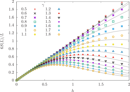
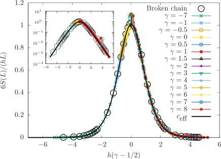
Figure 8: Top: Entropy per site of the rainbow model with a defect, $s(h,\gamma)$ as a function of $h$, for different values of $\gamma$. Soft continuous lines correspond to the theoretical prediction, Eq. (46). Bottom: entropy per site divided by the inhomogeneity parameter, as a function of the defect intensity, $h(\gamma-1/2)$, showing the collapse predicted by Eq. (46).

IV.4 Phase Diagram

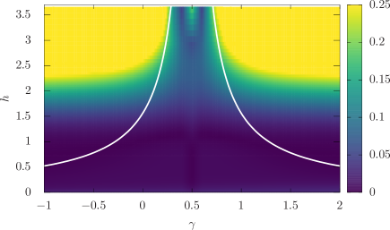
Figure 9: Phase diagram, absolute error of the EE prediction; the white lines correspond to the local maximum of the entropy density, $s(h)$.

In Fig. (9) we show the relative error between the theoretical prediction and the numerics

$$\delta s(h,\gamma)=\frac{|s(h,\gamma)-hc_{\text{eff}}|}{s(h,\gamma)},$$ (48)

in the color intensity. The white lines correspond to the theoretical values of the relative maxima of $s(h,\gamma)$ as a function of $h$, following Eq. (46). Notice that the theoretical prediction states that, for all $\gamma$, the curve $s(h)$ will present a maximum and decay to zero afterwards. Thus, weak inhomogeneity regime presents a smooth crossover into the three phases of the strong coupling regime described in the previous section. or large $h$ lattice effects become dominant and the universal properties predicted by the field theory approach are lost.

IV.5 Beyond Entanglement Entropy

The characterization of entanglement can be improved with the study of the entanglement spectrum (ES), entanglement contour and entanglement Hamiltonian. All these mathematical objects are associated to the reduced density matrix of the block, $\rho_{A}$.

IV.5.1 Entanglement Hamiltonian

The reduced density matrix $\rho_{A}$ of a Gaussian fermionic state can be written in the form

$$\rho_{A}=\exp(-2\pi H_{A})\equiv\exp\left(-2\pi\sum_{p}\epsilon_{p}d^{\dagger}_{p}d_{p}\right),$$ (49)

for some fermionic operators $d_{p}$. The $\epsilon_{p}$ are called the single-body entanglement spectrum, but the term single-body is usually dropped. Operator $H_{A}$ is termed the entanglement Hamiltonian (EH), and it can be shown to be approximately local for a 1+1D CFT Tonni.18 . Indeed, it can be written as

$$H_{A}\approx\sum_{i}\beta_{A}(i)\;c^{\dagger}_{i}c_{i+1},$$ (50)

where the $\beta_{A}(i)$ constitute entanglement couplings, and can be accounted for in CFT providing an extension of the Bisognano-Wichmann theorem Cardy.16 ; Tonni.18 . There are also non-zero terms presenting long-range interactions, but they are expected to be very small. The estimation of the set of $\beta_{i}$ is obtained by minimizing an error function $E(\beta)\equiv\sum_{i,j\in A}\left(C_{ij}-Tr(\rho_{A}(\beta)c^{\dagger}_{i}c_{j})\right)$ using standard optimization techniques Tonni.18 .

The numerical values of $\{\beta(i)\}$ for the left half (block $A_{L}$) of a $L=20$ system, using $h=0.5$ and different values of $\gamma$ are shown in Fig. 10. For $\gamma=1/2$ the EH of the rainbow system presents flat coefficients $\beta(i)$ everywhere except near the physical boundary (left extreme) and near the internal boundary (right extreme), where it follows the Bisognano-Wichmann prediction, that they will decay to zero linearly, with slope $1$. Yet, in presence of a defect we observe an increasing dimerization of the EH.

Let us remind the reader that the flat profile for $\{\beta(i)\}$ in the rainbow case accounts for the fact that the rainbow GS for all values of $h$ resembles a thermofield double Tonni.18 , i.e.

$$\ket{\Psi}\approx\sum_{n}\exp(-\beta E_{n}/2)\ket{n}_{L}\otimes\ket{n}_{R},$$ (51)

where $E_{n}$ and $\ket{n}_{\{L,R\}}$ are the energies and eigenstates of the homogeneous free Hamiltonian on the left/right with open boundaries. Thus, we are led to the following claim: in presence of a defect, the ground state of Hamiltonian (1) is still approximately a thermofield double, but of a dimerized Hamiltonian, with dimerization parameter associated to the defect strength $\gamma$.

We would like to stress that the cases of $\gamma$ and $1-\gamma$ are extremely similar, only interchanging the higher and lower values of the dimerization pattern.

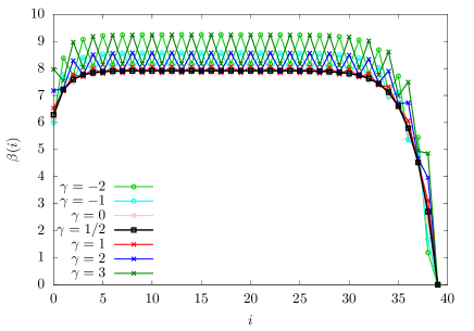
Figure 10: Entanglement Hamiltonian coefficients $\{\beta(i)\}$ for the left half of a $L=20$ rainbow with a defect, using $h=0.5$. Notice that, for $\gamma=1/2$ the bulk is flat, as expected, but for the other values the Hamiltonian coefficients present dimerization, which changes the high and low values when we change $\gamma$ for $1-\gamma$.

IV.5.2 Entanglement Spectrum

For free systems, the entanglement spectrum (ES) $\{\epsilon_{k}\}_{k=1}^{L}$ of a block $A$ is the single-body spectrum of the reduced density matrix $\rho_{A}$ Li_Haldane.08 . In terms of the ES, the eigenvalues $\{\nu_{k}\}_{k=1}^{L}$ of the block correlator matrix are written Peschel.03 as:

$$\nu_{k}=\frac{1}{e^{\epsilon_{k}}+1}.$$ (52)

The ES contains more physical information than the entanglement entropy. In some cases, its low part can be regarded as the energy spectrum of a boundary CFT Lauchli2013 .

We have considered the full ES of the left half block, $A_{L}$, for different values of $\gamma$. As it can be expected, the defect preserves the particle-hole symmetry. The most salient feature is that the ES shows a finite gap $\Delta\epsilon$ whose width grows with $\gamma$, as can be seen in Fig. 11 (top). For a CFT system, the entanglement gap, $\Delta\epsilon\sim 1/\log(L)$, but for a deformed system such as the rainbow we should consider instead $\Delta\epsilon\sim 1/\log(\tilde{L})\sim 1/L$. Indeed, for low $h$ the gap decays linearly with the system size, as we can see on the bottom panel of Fig. 11 for $h=0.015$, but it seems to reach a finite value for $h=0.32$.

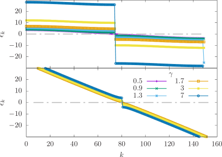
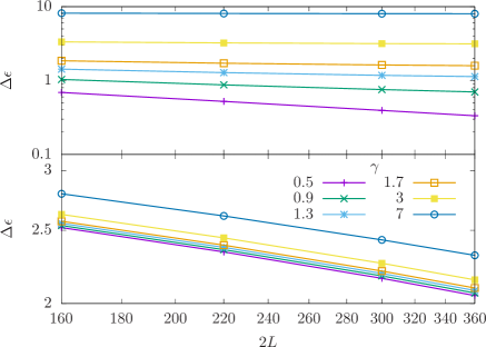
Figure 11: Top: Entanglement spectrum $\epsilon_{k}$ of the left block of a system with $L=150$ and different values of $\gamma$. Upper panel: $h=0.32$, lower panel: $h=0.015$. Bottom: Scaling of the ES gap $\Delta\epsilon$ with size $2L$ for different values of $\gamma$. The upper panel shows the case $h=0.32$, and the lower panel $h=0.015$.

IV.5.3 Entanglement Contour

The entanglement contour Vidal.14 attempts to answer the question about where is the entanglement entropy located. The entanglement entropy of a block is decomposed

$$S_{A}=\sum_{i\in A}\sigma_{A}(i),$$ (53)

with $\sigma_{A}(i)\geq 0$. Although the entanglement contour is not uniquely defined, different candidate definitions have provided very similar values Coser.17 ; Tonni.18 ; Roy.19 , thus pointing at the existence of a deeper contour which would have the current candidates as approximations. Since the rainbow system is defined here for a free-fermionic system, we will employ the approach given in Vidal.14 .

Fig. 12 shows the curve of the entanglement contour for the left block of the rainbow GS using $L=40$ and $h=0.5$, for different values of $\gamma$, scaled with the entropy density predicted in Eq. (46). The collapse is very clear in the bulk region, which presents universal features, and a little bit less near the boundary, where it does not. Importantly, notice that the entanglement contour does not present any oscillations related to dimerization, with a constant entropy per site in the bulk.

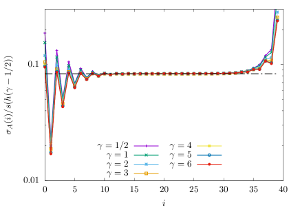
Figure 12: Entanglement contour of the left half (the left edge is the physical boundary while the right one is originated by the block) of the rainbow model with a defect using $L=40$ and $h=0.5$, scaled with the entropy per site predicted in Eq. (46), for different values of $\gamma$.

V Defect in a symmetry protected topological phase

The system considered so far, Eq. (1), presents bond centered symmetry, i.e.: the center of symmetry is in the middle point of the central link. However, many different properties arise when we consider site centered symmetric (scs) systems Samos.19 , where the center of symmetry corresponds to a site. Let us consider a system defined on a chain with $N=2L$ sites, whose Hamiltonian is:

$$H_{N}(h,\gamma)_{\text{scs}}=-\frac{1}{2}\sum_{m=1}^{N}J_{m}c_{m}^{\dagger}c_{m+1}+\text{h.c.},$$ (54)

where the fermions are now placed on integer positions and there are two equal central hoppings depending on $\gamma$:

$$J_{m}=\begin{cases}e^{-h(\left|m-(L+\frac{1}{2})\right|-\frac{1}{2})}&\text{if }m\neq L,L+1,\\ e^{-h\gamma}&\text{if }m\in\{L,L+1\},\end{cases}$$ (55)

i.e., the log-couplings (see Eq. (7)) present the pattern $\{\dots,3,2,1,\gamma,\gamma,1,2,3,\dots\}$. The site-centered symmetry manifests itself through the invariance of the hoppings under an inversion around the central site $L+1$: $J_{n}=J_{L+1-n}$. Notice that the new notation is different from the bond centered symmetry case, Eq. (1), which is now convenient due to the different type of symmetry.

In Samos.19 it was shown that after performing a folding operation around the central site, the system becomes an inhomogeneous realization of the SSH model, thus belonging to the BDI class of topological phases Kennedy1992 ; Altland1997 ; P10 ; Fidkowski2011 ; Turner2011 ; W11a ; W11b ; P12 . Since the topological nature of the state is highlighted after removing the local entanglement W11b , it is better to study the system in the strong inhomogeneity regime. The fermionic excitations are not spread along the whole system as it is the case in the weak inhomogeneity limit. Hence, we will study the system in the strong coupling regime $H_{N}(h\gg 1,\gamma)_{\text{scs}}$ by means of renormalization schemes that depend on the value of $\gamma$ (see details in Appendix E).

Let us start by considering the case $\gamma\leq 1$. The dominant interaction involves the three central sites, $L$, $L+1$ and $L+2$. With a real space first order perturbation theory RG Samos.19 . On each step, three fermions are truncated into one which participates on the next step (unlike the RG of the systems with bcs symmetry, where the fermions are integrated out on each step and hence are decoupled from the system) leading to a topological ground state with non removable entanglement that belongs to the BDI class Altland1997 ; Samos.19 . The case with $\gamma=1$ differs only on the first step of the RG where 5 spins (instead of three) are truncated to one.
On the other hand, the case $\gamma>1$ is again different. Starting from $H_{N}(h,\gamma)_{\text{scs}}$, the dominant interactions are two non consecutive log-couplings 1 which allows the use of the Dasgupta-Ma RG Eq. (8), leading to an effective system whose Hamiltonian is $H_{N-4}(h,1+\gamma)_{\text{scs}}$. If $1+\gamma$ happens to be the dominant interaction, three fermions are involved so the Dasgupta-Ma Rg is not applicable anymore and the way of procedure is described in the previous paragraph. On the contrary, if the log-couplings 2 are the dominant interaction, the Dasgupta-Ma RG can be applied again leading to a new Hamiltonian $H_{N-8}(h,2+\gamma)_{\text{scs}}$. Hence, the same dichotomy is present in the next step. The procedure iterates and unless $\gamma>L-1$ the RG flows eventually to a dominant interaction which involves three fermions.

Therefore we see that the GS of the Hamiltonian $H_{N}(h,\gamma>1)_{\text{scs}}$ is obtained via the application of two kinds of renormalization group schemes. As a consequence, the ground state of this Hamiltonian has two different phases that coexist: a dimerized phase around the defect and the BDI phase away from it. This coexistence is well captured by considering the EE of central blocks $B_{\ell}=\{L-\ell,L+2+\ell\}$, with $\ell\in\{0,\dots,(L-1)\}$. Since the system is topologically non-trivial, there is entanglement that cannot be removed (the EE in bounded by $\log 2$ for all $B_{\ell}$) and for blocks $B_{\ell}$ with $\ell<\lfloor\gamma\rfloor$, $S{B_{\ell}}=3\log{2}$ due to the fact that there are two fermionic excitations $b_{L-2(\ell-1),L-2(\ell-1)-1}^{\dagger}\ket{0}$ and $b_{L+2\ell,L+2\ell+1}^{\dagger}\ket{0}$ that are not fully contained in the block $B_{\ell}$. Furthermore, the dimerized phase appears only in the strong coupling limit $h\to\infty$ while the BDI phase is independent of the inhomogeneity parameter. This fact can be checked by considering the behaviour of the single body entanglement spectrum $\epsilon_{k}$, see Fig. 13 and Eq. (52). There is a zero mode $\epsilon_{0}=0$ for all $h$ that gives rise to a double degeneracy of the many-body entanglement spectrum and it is a signature of the topological nature of the state. There are also two additional zero modes due to the presence of the defect but they are not topological, since they depend on the inhomogeneity.

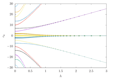
Figure 13: Single body entanglement spectrum $\epsilon_{k}$ of a block $B_{11}$ of a system described by the Hamiltonian $H_{46}(h,\frac{17}{2})_{\text{scs}}$ as a function of $h$. Notice the topological zero mode, which does not depend on $h$.

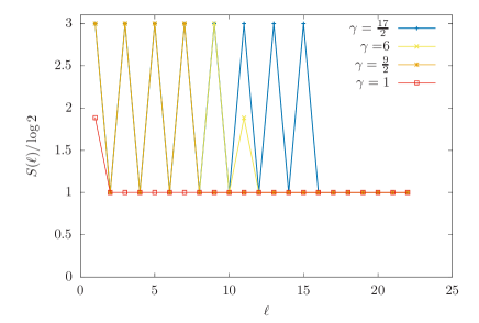
Figure 14: Entanglement entropy of the system with Hamiltonian $H_{46}(15,\gamma)_{\text{scs}}$ partitioned with central blocks $B_{\ell}$ for different values of $\gamma$. The entropy is $S[B_{\ell}]=3\log 2$ if $\ell<\lfloor\gamma\rfloor$ and it is $S[B_{\ell}]=\log 2$ if $\ell>\lfloor\gamma\rfloor$. If $\gamma\in\mathbb{N}$, $S[B_{\ell=\gamma}]$ takes another value which is a consequence of the quadruple tie that we have discussed in the text.

VI Conclusions and further work

In this work we have characterized a lattice model of Dirac fermions on a negatively curved background in presence of a local defect. The unperturbed lattice model is the so-called rainbow model, which is a free-fermionic chain with hoppings which decay exponentially from the center. Its ground state presents linear growth of the entanglement, with an entropy per site proportional to the inhomogeneity parameter $h$ in the weak inhomogeneity regime, which is described by a geometrical deformation of the free-fermionic conformal field theory, associated to a hyperbolic space-time metric. The strong inhomogeneity limit is described as a valence bond state with concentric bonds around the center, as it can be established using the Dasgupta-Ma renormalization group.

The presence of a defect in the center of the chain can induce an entanglement transition in the strong inhomogeneity limit, characterized by a rainbow phase of linear scaling of entanglement for intermediate defect strengths, and two dimerized phases, with alternate dimerizations in similarity with the SSH model. Further hints of the transition are provided by the ground state energy, the single-body orbitals, the energy gap (rescaled with the minimum coupling) and two order parameters: the average dimerization and the rainbow order parameter, which measures the average occupation of the concentric bonds.

In the weak inhomogeneity limit, the transition gets blurred, and the ground state always presents linear entanglement, with an entropy per site that can be effectively described by a geometric deformation of the entanglement entropy of a homogeneous fermionic chain with a central defect. Analysis of the entanglement gap and the entanglement Hamiltonian allow us to claim that the system behaves as a thermofield double, as in the rainbow case, but with a dimerized Hamiltonian instead of a homogeneous one.

Interestingly, the rainbow system presents non-trivial topological properties when it is centered on a site instead of a link. In presence of a defect, the ground state presents an interesting coexistence of a symmetry-protected topological phase near the ends and a dimerized region near the center, whose size grows as the defect intensity goes to zero.

Our work opens up several interesting questions related to the presence of geometric defects on the vacuum structure of a quantum field theory. It is interesting to ask whether such a deep modification of the entanglement properties can be found in other cases.

Appendix A Dasgupta-Ma RG extension for free fermions

In this Appendix we describe a generalization of the Dasgupta-Ma RG for inhomogeneous free fermionic chains that can be applied to systems that have an homogeneous subchain of $N=2L$ sites embedded. The Hamiltonian $H_{0}$ that describes this subchain is given by

$$H_{0}=-\frac{J}{2}\sum_{i=1}^{N-1}c_{i}^{\dagger}c_{i+1}+c_{i+1}^{\dagger}c_{i},$$ (56)

and its interactions with the nearest neighbours is given by $H_{lr}$

$$H_{lr}=-J_{l}c_{l}^{\dagger}c_{1}-J_{r}c_{N}^{\dagger}c_{r}+\text{h.c.}.$$ (57)

Assuming that $J_{l}\ll J$ and $\frac{J_{l}}{J_{r}}\approx 1$ the whole system can be study by means of degenerate perturbation theory. The ground state of $H_{0}$ is given in the previous Appendix B $\ket{\psi_{0}}=\prod_{m=1}^{L}\hat{\phi}_{k_{m}}^{\dagger}\ket{0}$ with energy $E_{0}=\sum_{m=1}^{L}\epsilon_{k_{m}}=-2\sum_{m=1}^{L}\cos\left(\frac{m\pi}{N+1}\right)$. The first order correction $\langle\psi_{0};l^{\prime},r^{\prime}|H_{lr}|\psi_{0};l,r\rangle$ (where $\ket{\psi_{i};l,r}=\ket{\psi_{i}}\otimes\ket{l}\otimes\ket{r}$) vanishes. The matrix element $B_{l,r;l^{\prime}r^{\prime}}$ of the degenerate second order contribution is given by:

$$B_{l,r;l^{\prime}r^{\prime}}=\sum_{i\neq 0}\sum_{l^{\prime\prime}r^{\prime\prime}}\frac{\langle\psi_{0};l,r|H_{lr}|\psi_{i};l^{\prime\prime},r^{\prime\prime}\rangle\langle\psi_{i};l^{\prime\prime},r^{\prime\prime}|H_{lr}|\psi_{0};l^{\prime},r^{\prime}\rangle}{E_{0}-E_{i}}$$ (58)

Expanding this product and taking into account that $\sum_{l^{\prime\prime}r^{\prime\prime}}\ket{l^{\prime\prime},r^{\prime\prime}}\bra{l^{\prime\prime},r^{\prime\prime}}=\mathbb{I}$ we have:

$$B_{l,r;l^{\prime}r^{\prime}} =J_{l}^{2}\left(\langle l,r|c_{l}^{\dagger}c_{l}|l^{\prime},r^{\prime}\rangle\sum_{i=1}^{N}\dfrac{\langle\psi_{0}|c_{1}|\psi_{i}\rangle\langle\psi_{i}|c_{1}^{\dagger}|\psi_{0}\rangle+\langle\psi_{0}|c_{1}^{\dagger}|\psi_{i}\rangle\langle\psi_{i}|c_{1}|\psi_{0}\rangle}{\epsilon_{k_{i}}}-\sum_{i=1}^{N}\dfrac{\langle\psi_{0}|c_{1}^{\dagger}|\psi_{i}\rangle\langle\psi_{i}|c_{1}|\psi_{0}\rangle}{\epsilon_{k_{i}}}\right)+$$ (59)

$$J_{r}^{2}\left(\langle l,r|c_{r}^{\dagger}c_{r}|l^{\prime},r^{\prime}\rangle\sum_{i=1}^{N}\dfrac{\langle\psi_{0}|c_{N}|\psi_{i}\rangle\langle\psi_{i}|c_{N}^{\dagger}|\psi_{0}\rangle+\langle\psi_{0}|c_{N}^{\dagger}|\psi_{i}\rangle\langle\psi_{i}|c_{N}|\psi_{0}\rangle}{\epsilon_{k_{i}}}-\sum_{i=1}^{N}\dfrac{\langle\psi_{0}|c_{N}^{\dagger}|\psi_{i}\rangle\langle\psi_{i}|c_{N}|\psi_{0}\rangle}{\epsilon_{k_{i}}}\right)+$$

$$J_{l}J_{r}\left(\langle l,r|c_{l}^{\dagger}c_{r}|l^{\prime},r^{\prime}\rangle\sum_{i=1}^{N}\dfrac{\langle\psi_{0}|c_{1}|\psi_{i}\rangle\langle\psi_{i}|c_{N}^{\dagger}|\psi_{0}\rangle+\langle\psi_{0}|c_{N}^{\dagger}|\psi_{i}\rangle\langle\psi_{i}|c_{1}|\psi_{0}\rangle}{\epsilon_{k_{i}}}+\right.$$

$$\left.\langle l,r|c_{r}^{\dagger}c_{l}|l^{\prime},r^{\prime}\rangle\sum_{i=1}^{N}\dfrac{\langle\psi_{0}|c_{N}|\psi_{i}\rangle\langle\psi_{i}|c_{1}^{\dagger}|\psi_{0}\rangle+\langle\psi_{0}|c_{1}^{\dagger}|\psi_{i}\rangle\langle\psi_{i}|c_{N}|\psi_{0}\rangle}{\epsilon_{k_{i}}}\right)$$

Where the non vanishing contributions are given by the excited states whose particle number differs by one with respect to $\ket{\psi_{0}}$:

$$\langle\psi_{i}|c_{i}^{\dagger}|\psi_{0}\rangle\neq 0\quad\text{if}\quad\ket{\psi_{i}}=\hat{\phi}_{k_{i}}\ket{\psi_{0}},\quad E_{i}=E_{0}-\epsilon_{k_{i}},$$ (60)

$$\langle\psi_{i}|c_{i}|\psi_{0}\rangle\neq 0\quad\text{if}\quad\ket{\psi_{i}}=\hat{\phi}_{k_{i}}^{\dagger}\ket{\psi_{0}},\quad E_{i}=E_{0}+\epsilon_{k_{i}}\ .$$ (61)

Given that $c_{i}=\sum_{m=1}^{N}f^{*}_{im}\hat{\phi}_{k_{m}}$ we reach

$$B_{l,r;l^{\prime}r^{\prime}}=J_{l}^{2}\left(\langle l,r|c_{l}^{\dagger}c_{l}|l^{\prime},r^{\prime}\rangle\sum_{i=1}^{N}\dfrac{|f_{1m}|^{2}}{\epsilon_{k_{m}}}+\sum_{i=1}^{L}\dfrac{|f_{1m}|^{2}}{\epsilon_{k_{m}}}\right)+J_{r}^{2}\left(\langle l,r|c_{r}^{\dagger}c_{r}|l^{\prime},r^{\prime}\rangle\sum_{i=1}^{N}\dfrac{|f_{Nm}|^{2}}{\epsilon_{k_{m}}}+\sum_{i=1}^{L}\dfrac{|f_{Nm}|^{2}}{\epsilon_{k_{m}}}\right)+$$

$$J_{l}J_{r}\left(\langle l,r|c_{l}^{\dagger}c_{r}|l^{\prime},r^{\prime}\rangle\sum_{i=1}^{N}\dfrac{f_{1m}^{*}f_{mN}}{\epsilon_{k_{m}}}+\langle l,r|c_{r}^{\dagger}c_{l}|l^{\prime},r^{\prime}\rangle\sum_{i=1}^{N}\dfrac{f_{Nm}^{*}f_{m1}}{\epsilon_{k_{m}}}\right).$$

Now, particularizing for the functions Eq. (63) we obtain that the renormalized Hamiltonian $B$ is (up to an additive constant):

$$H_{eff}=-\frac{J_{l}J_{r}}{J}\left(c_{l}^{\dagger}c_{r}+\text{h.c}\right),$$ (62)

which is the expression used to renormalize the systems with strength defects $\gamma=0$ and $\gamma=1$.

Appendix B The transition blocks: $\gamma=1$ and $\gamma=0$.

In this appendix we derive Eq. (15). Consider an homogeneous system of $N=2L$ sites with open boundary conditions (OBC) whose Hamiltonian is given by Eq. (56). Solving the time independent Schrödinger equation $H_{0}\ket{\phi_{k}}=\epsilon_{k}\ket{\phi_{k}}$ we arrive at

$$\epsilon_{k_{m}} = -J\cos\left(\frac{m\pi}{N+1}\right)$$ (63)

$$\ket{\phi_{k_{m}}} = \hat{\phi}_{k_{m}}^{\dagger}\ket{0}=\sum_{i=1}^{N}f^{*}_{mi}c_{i}^{\dagger}\ket{0},\quad\text{within }f^{*}_{mi}=\sqrt{\frac{2}{N+1}}\sin\left(\frac{m\pi i}{N+1}\right).$$

Taking $N=4$, the many body ground state $\ket{\psi}$ at half filling is obtained by occupying the single body levels with energies $-J\cos\frac{\pi}{5}$ and $-J\cos\frac{2\pi}{5}$.

$$\ket{\psi_{0}}=d^{\dagger}\ket{0}=v^{\dagger}u^{\dagger}\ket{0}=\hat{\phi}_{k_{2}}^{\dagger}\hat{\phi}_{k_{1}}^{\dagger}\ket{0}.$$ (64)

Appendix C Correlation matrices and entanglement entropy

The correlation matrices $C$ for the ground states Eqs. (10)-(14) are given by

$$C_{ij} = \langle GS|c^{\dagger}_{i}c_{j}|GS\rangle=\sum_{m,m^{\prime}=1}^{L}f_{i,m}f_{m^{\prime},j}^{*}\langle GS|\hat{\phi}_{m}^{\dagger}\hat{\phi}_{m^{\prime}}|GS\rangle$$ (65)

$$= \sum_{m=1}^{L}f_{i,m}f_{m,j}^{*},$$

where we consider half filling and $\hat{\phi}_{m}$ are the fermionic excitations of each system ($b_{i,j}$ Eq. (6) and $d_{i}$ Eq. (15) in our case) and $f_{i,k}$ is a unitary matrix.

The EE entropy of a block $A_{\ell}$ is given by Peschel.03 :

$$S(A_{\ell})=-\sum_{k=1}^{\ell}\nu_{k}\log{\nu_{k}}+(1-\nu_{k})\log{(1-\nu_{k})},$$ (66)

where the $\{\nu_{k}\}$ are the set of eigenvalues of the correlation matrix restricted to the block $A_{\ell}$. We shall next describe the correlation matrices as a function of the defect parameter $\gamma$. All the matrices are symmetric $C_{i,j}=C_{j,i}$ and present left-right symmetry $C_{i,j}=C_{N+1-j,N+1-i}$. All the computations are done with $L$ even.

• $\gamma<0$:

  $$\begin{cases}C_{i,i}=\frac{1}{2},\quad i=1,\dots,L\\ C_{1,N}=-\frac{1}{2},\\ C_{2i,2i+1}=\frac{1}{2},\quad i=1,\dots\frac{L}{2},\end{cases}$$ (67)

• $\gamma=0$:

  $$\begin{cases}C_{1,N}=-\frac{1}{2},\quad C_{L,L+1}=\frac{1}{2}\\ C_{i,i}=\frac{1}{2},\quad i=1,\dots,L\\ C_{i,N+1-i}=(-1)^{i}\frac{1}{2\sqrt{5}},\quad i=2,\dots,L-1\\ C_{2i,2i+1}=\frac{1}{\sqrt{5}},\quad i=1,\dots\frac{L}{2},\end{cases}$$ (68)

• $\gamma\in(0,1)$:

  $$C_{i,j} = \frac{1}{2}\delta_{i,i}+(-1)^{i}\frac{1}{2}\delta_{i,N+1-i},$$ (69)

• $\gamma=1$:

  $$\begin{cases}C_{i,i}&=\frac{1}{2},\quad i=1,\dots,L\\ C_{i,N+1-i}&=(-1)^{i}\frac{1}{2\sqrt{5}},\quad i=1,\dots,L\\ C_{2i-1,2i}&=\frac{1}{\sqrt{5}},\quad i=1,\dots\frac{L}{2}\end{cases}$$ (70)

• $\gamma>1$:

  $$\begin{cases}C_{i,i}=\frac{1}{2},\quad&i=1,\dots,L\\ C_{2i-1,2i}=\frac{1}{2},\quad&i=1,\dots\frac{L}{2}\end{cases}$$ (71)

  The correlation matrix of the four sites that are integrated out in the same step whose ground state is given by Eq. (15) is

  $$C_{4}=\left(\begin{array}[]{cccc}\frac{1}{2}&\frac{1}{\sqrt{5}}&0&-\frac{1}{2\sqrt{5}}\\ \frac{1}{\sqrt{5}}&\frac{1}{2}&\frac{1}{2\sqrt{5}}&0\\ 0&\frac{1}{2\sqrt{5}}&\frac{1}{2}&\frac{1}{\sqrt{5}}\\ -\frac{1}{2\sqrt{5}}&0&\frac{1}{\sqrt{5}}&\frac{1}{2}\\ \end{array}\right).$$ (72)

  The most simple non trivial lateral block is

  $$A_{2}=\left(\begin{array}[]{cc}\frac{1}{2}&\frac{1}{\sqrt{5}}\\ \frac{1}{\sqrt{5}}&\frac{1}{2}\\ \end{array}\right),$$ (73)

  whose eigenvalues are $\nu_{1}=\frac{1}{10}\left(2\sqrt{5}+5\right),\nu_{2}=\frac{1}{10}\left(5-2\sqrt{5}\right)$. The value of $S_{a}$, given in Eq. (25), is obtained applying Eq. (66). Furthermore $S_{b}$, given in Eq. (26, is obtained from the central block

  $$B_{1}=\left(\begin{array}[]{cc}\frac{1}{2}&\frac{1}{2\sqrt{5}}\\ \frac{1}{2\sqrt{5}}&\frac{1}{2}\\ \end{array}\right),$$ (74)

  whose eigenvalues are $\nu_{1}=\frac{1}{10}\left(\sqrt{5}+5\right),\nu_{2}=\frac{1}{10}\left(5-\sqrt{5}\right)$. It can be shown that larger central blocks have also these non trivial eigenvalues and the rest are 0 and 1 which don’t contribute to the EE.

Appendix D Relation with Dirac equation with $\delta$ potential

Consider an inhomogeneous free-fermion chain with a central hopping defect and bond centered symmetry described by the Hamiltonian:

$$H(\tau)=-\frac{\tau}{2}c_{-\frac{1}{2}}^{\dagger}c_{\frac{1}{2}}-\frac{1}{2}\sum_{m=\frac{1}{2}}^{L-\frac{3}{2}}J_{m}\left(c^{\dagger}_{m}c_{m+1}+c^{\dagger}_{-m}c_{-m+1}\right).$$ (75)

The single body spectrum is obtained by diagonalizing the hopping matrix. The eigenvalue equations at the center of the chain are

$$\alpha\phi_{-\frac{3}{2}}+\tau\phi_{\frac{1}{2}} = \epsilon\phi_{-\frac{1}{2}}$$ (76)

$$\tau\phi_{-\frac{1}{2}}+\alpha\phi_{\frac{3}{2}} = \epsilon\phi_{\frac{1}{2}}$$ (77)

where $\epsilon$ is the single body energy and $\phi_{m}$ is the amplitude associated with the fermionic operator $c_{m}$ and $J_{\frac{1}{2}}=\alpha$. The expansion of the local operators $c_{m}$ in terms of its right and left moving components around the Fermi points (see Eq. (28)) leads to the equations:

$$\tau\left(\psi_{L}^{II}-i\psi_{R}^{II}\right) =\left(-i\epsilon+\alpha\right)\psi_{L}^{I}+\left(\epsilon-i\alpha\right)\psi_{R}^{I}$$ (78)

$$\tau\left(\psi_{L}^{I}+i\psi_{R}^{I}\right) =\left(i\epsilon+\alpha\right)\psi_{L}^{II}+\left(\epsilon+i\alpha\right)\psi_{R}^{II},$$ (79)

with

$$\lim_{a\to 0}\psi_{L,R}\left(-\frac{3}{2}a\right) = \lim_{a\to 0}\psi_{L,R}\left(-\frac{1}{2}a\right)=\psi_{L,R}^{I},$$ (80)

$$\lim_{a\to 0}\psi_{L,R}\left(\frac{3}{2}a\right) = \lim_{a\to 0}\psi_{L,R}\left(\frac{1}{2}a\right)=\psi_{L,R}^{II},$$ (81)

Solving for $\psi_{L}^{I}$ in Eq. (78) and putting it into Eq. (79) we have:

$$\psi_{R}^{I}=\frac{1}{2\alpha\tau}\left(i(\tau^{2}-\alpha^{2}-\epsilon^{2})\psi_{L}^{II}+(\tau^{2}-(\epsilon+i\alpha)^{2})\psi_{R}^{II}\right).$$ (82)

Inserting this expression into Eq. (78) we arrive at

$$\psi_{L}^{I}=\frac{1}{2\alpha\tau}\left((\tau^{2}+(\alpha+i\epsilon)^{2})\psi_{L}^{II}-i(\tau^{2}-\alpha^{2}+\epsilon^{2})\psi_{R}^{II}\right).$$ (83)

We can express these two equations as $\psi^{I}=T\psi^{II}$, where $T$ is a transfer matrix:

$$\begin{pmatrix}\psi_{L}^{I}\\ \psi_{R}^{I}\end{pmatrix}=\frac{1}{2\alpha\tau}\begin{pmatrix}\tau^{2}+(\alpha+i\epsilon)^{2}&-i(\tau^{2}-\alpha^{2}+\epsilon^{2})\\ i(\tau^{2}-\alpha^{2}-\epsilon^{2})&\tau^{2}-(\epsilon+i\alpha)^{2}\end{pmatrix}\begin{pmatrix}\psi_{L}^{II}\\ \psi_{R}^{II}\end{pmatrix}.$$ (84)

Furthermore, at half filling we have that $\epsilon\xrightarrow[L\to\infty]{}0$ and the transfer matrix simplifies to:

$$T=\frac{1}{2\alpha\tau}\begin{pmatrix}\tau^{2}+\alpha^{2}&-i(\tau^{2}-\alpha^{2})\\ i(\tau^{2}-\alpha^{2})&\tau^{2}+\alpha^{2}\end{pmatrix}.$$ (85)

Note that this can be also written as:

$$T=\frac{1}{2\tilde{\tau}}\begin{pmatrix}\tilde{\tau}^{2}+1&-i(\tilde{\tau}^{2}-1)\\ i(\tilde{\tau}^{2}-1)&\tilde{\tau}^{2}+1\end{pmatrix},$$ (86)

where $\tilde{\tau}=\frac{\tau}{\alpha}$. Substituting $\tau=e^{-h\gamma}$ and $\alpha=e^{-\frac{h}{2}}$ we have the expression Eq. (35).

Appendix E Details of the RG applied to the SCS system

In this Appendix we derive the ground state of the Hamiltonian

$$H_{N}(h,\gamma)_{\text{scs}}=-\frac{1}{2}\sum_{m=1}^{N}J_{m}c_{m}^{\dagger}c_{m+1}+\text{h.c.},\quad\text{with}\quad J_{m}=\begin{cases}e^{-h(\left|m-(L+\frac{1}{2})\right|-\frac{1}{2})}&\text{if }m\neq L,L+1,\\ e^{-h\gamma}&\text{if }m\in\{L,L+1\}\ .\end{cases}$$ (87)

We use the RG scheme explained in the main text. There are three cases to be considered:

(1.-) Case $\gamma<1$. The couplings present a double tie at the center, so that the dominant interaction involves the three central sites, $L$, $L+1$ and $L+2$. The Dasgupta-Ma prescription Eq. (8) and the sum rule Eq. (9) are not valid in this situation. We must perform a first order perturbation approach to renormalize three fermionic sites into an effective site (see Appendix A of Samos.19 ), leading to a system with $N-2$ sites. The next RG step involves the effective fermion mode created on the previous one and its two nearest neighbours. Iterating this procedure one obtains the GS:

$$\ket{GS}_{\gamma<1}=(g^{\xi}_{L})^{\dagger}\prod_{m=1}^{L-2}(f^{s_{m}}_{m})^{\dagger}(g^{+}_{0})^{\dagger}\ket{0},$$ (88)

where $s_{m}=(-1)^{m}$, $\xi=(-1)^{\frac{L}{2}}$ and

$$g^{\pm}_{m} = \frac{1}{\sqrt{2}}(c_{L+1}+b^{\pm}_{L-2m,L+2(m+1)}),$$ (89)

$$g^{\pm}_{L} = \frac{1}{\sqrt{2}}(c_{1}+b^{\pm}_{2,2L})$$ (90)

$$f^{\pm}_{n} = \frac{1}{\sqrt{2}}(b^{\pm}_{L+1-n,L+1+n}+b^{\pm}_{L-n,L+2+n}),$$ (91)

with $b^{\pm}_{i,j}$ defined in Eq. (6).

(2.-) Case $\gamma=1$. The system presents a quadruple tie at the center. The five central sites involved are renormalized into an effective site on a system with $N-4$ sites. At this point the situation is equivalent to the $\gamma<1$ case and further RG steps are the same as the ones discussed in the previous item.

(3.-) Case $\gamma>1$. In this situation, the dominant interactions are two non-consecutive log-couplings 1, which couple respectively the sites $L-1$ and $L$, and the sites $L+2$ and $L+3$. Although the sum rule Eq. (9) is not valid, the Dasgupta-Ma Eq. (8) can be applied sequentially twice, yielding two fermionic excitations with the same energy and parity, $b^{+}_{L-1,L}$ and $b^{+}_{L+2,L+3}$, and leading to a effective system whose Hamiltonian is $H_{N-4}(h,1+\gamma)_{\text{scs}}$. The next decimation step is not univocal:

• If $\gamma\in(1,2)$ the dominant interaction involves the three central sites $L-2$,$L$ and $L+4$ of the original chain and the situation is the same as the one described originally for $\gamma<1$, with the double tie (1.).

• If $\gamma=2$ there is a quadruple tie, same as (2.).

• If $\gamma\in(2,3)$ the dominant interactions are the two links with log-coupling 3, which is similar to the situation described in item (3.). At the end of this step there are two fermionic excitations more, $b^{+}_{L-3,L-2}$ and $b^{+}_{L+4,L+5}$, and the Hamiltonian of the decimated system is $H_{N-8}(h,2+\gamma)_{\text{scs}}$. We show in Fig. 15 this situation.

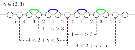
Figure 15: RG procedure for a system $H_{N}(h,\gamma)_{\text{scs}}$ with $h\gg 1$ and $\gamma\in(2,3)$. The system admits two Dasgupta-Ma RG steps, above links with log-coupling $1$, and after those the renormalized system shows a double tie of lowest log-couplings, with the two central log-couplings equal to $1+\gamma$ (which must be larger than $3$). At this moment, we apply the same RG procedure than for $\gamma<1$.

Note that unless $\gamma>L-1$ the RG flows towards the double tie situation and, if $\gamma\in\mathbb{N}$, the decimated system of the $\gamma$-th step will present a quadruple tie. Hence, the GS is:

$$\ket{GS}_{\gamma>1}=(g_{L}^{-})^{\dagger}\prod_{k=1}^{L-2(1+\lfloor\gamma\rfloor)}(f^{\eta_{k}}_{k+2\lfloor\gamma\rfloor})^{\dagger}(g^{-}_{\lfloor\gamma\rfloor})^{\dagger}\prod_{m=1}^{\lfloor\gamma\rfloor}(b^{+}_{L-2(m-1),L-2(m-1)-1})^{\dagger}(b^{+}_{L+2m,L+2m+1})^{\dagger}\ket{0},$$ (92)

where $\lfloor\rfloor$ is the floor function, $\eta_{k}=(-1)^{k+1}$, $\chi_{k}=(-1)^{k-\lfloor\gamma\rfloor}$.

References

- (1) L Amico, R Fazio, A Osterloh, V Vedral, Entanglement in many-body systems, Rev. Mod. Phys. 80, 517 (2008).
- (2) N Laflorencie, Quantum entanglement in condensed matter systems, Phys. Rep. 643, 1 (2016).
- (3) M Sredniki, Entropy and area, Phys. Rev. Lett. 71, 666 (1993).
- (4) J Eisert, M Cramer, MB Plenio, Area-laws for the entanglement entropy: a review, Rev. Mod. Phys. 82, 277 (2010).
- (5) C Holzhey, F Larsen, F Wilczek, Geometric and renormalized entropy in conformal field theory, Nucl. Phys. B 424, 443 (1994).
- (6) G Vidal, JI Latorre, E Rico, A Kitaev, Entanglement in quantum critical phenomena, Phys. Rev. Lett. 90 227902 (2003).
- (7) P Calabrese, JL Cardy, Entanglement entropy and quantum field theory, JSTAT P06002 (2004).
- (8) P Calabrese, J Cardy, Entanglement entropy and conformal field theory, J. Phys. A 42, 504005 (2009).
- (9) G Refael, JE Moore, Entanglement Entropy of Random Quantum Critical Points in One Dimension, Phys. Rev. Lett. 93, 260602 (2004).
- (10) G Refael, JE Moore, Criticality and entanglement in random quantum systems, J. Phys. A 42, 504010 (2009).
- (11) N. Laflorencie, Scaling of entanglement entropy in the random singlet phase Phys. Rev. B 72, 140408 (2005).
- (12) M Fagotti, P Calabrese, JE Moore, Entanglement spectrum of random-singlet quantum critical points, Phys. Rev. B 83, 045110 (2011).
- (13) G Ramírez, J Rodríguez-Laguna, G Sierra, Entanglement in low-energy states of the random coupling model, JSTAT P07003 (2014).
- (14) P Ruggiero, V Alba, P Calabrese, The entanglement negativity in random spin chains, Phys. Rev. B 94, 035152 (2016).
- (15) R. Vasseur, A. C. Potter, Yi-Zhuang and A. W. W. Ludwig, Entanglement Transitions from Holographic Random Tensor Networks, arXiv 1807.07082 (2018)
- (16) C. Dasgupta and S.-K. Ma, Low-temperature properties of the random Heisenberg antiferromagnetic chain, Phys. Rev. B 22, 1305 (1980).
- (17) D.S. Fisher, Critical behavior of random transverse-field Ising spin chains, Phys. Rev. B 51, 6411 (1995).
- (18) G. Vitagliano, A. Riera, and J. I. Latorre, Volume-law scaling for the entanglement entropy in spin 1/2 chains, New J. Phys. 12, 113049 (2010).
- (19) G. Ramírez, J. Rodríguez-Laguna and G. Sierra, From conformal to volume-law for the entanglement entropy in exponentially deformed critical spin 1/2 chains, J. Stat. Mech. P10004 (2014).
- (20) G. Ramírez, J. Rodríguez-Laguna and G. Sierra, Entanglement over the rainbow, J. Stat. Mech. P06002 (2015).
- (21) N Samos Sáenz de Buruaga, SN Santalla, J Rodríguez-Laguna, G Sierra, Symmetry protected phases in inhomogeneous spin chains, JSTAT 093102 (2019).
- (22) J. Rodríguez-Laguna, S.N. Santalla, G. Ramírez, G. Sierra, Entanglement in correlated random spin chains, RNA folding and kinetic roughening, New J. Phys. 18, 073025 (2016).
- (23) J. Rodríguez-Laguna, J. Dubaîl, G. Ramírez, P. Calabrese, G. Sierra, More on the rainbow chain: entanglement, space-time geometry and thermal states, J. Phys. A 50, 164001 (2017).
- (24) E. Tonni, J. Rodríguez-Laguna and G. Sierra, Entanglement hamiltonian and entanglement contour in inhomogeneous 1D critical systems, J. Stat. Mech. 043105 (2018).
- (25) I. MacCormack, A.L. Liu, M. Nozaki, S. Ryu, Holographic Duals of Inhomogeneous Systems: The Rainbow Chain and the Sine-Square Deformation Model, ArXiv:1812.10023 (2018).
- (26) R.N. Alexander, A. Ahmadain, Z. Zhang and I. Klich, Holographic rainbow networks for colorful Motzkin and Fredkin spin chains, arXiv:1811.11974.
- (27) V. Alba, S. N. Santalla, P. Ruggiero, J. Rodríguez-Laguna, P. Calabrese and G. Sierra, Unsual area-law violation in random inhomogeneous systems, JSTAT 023105 (2019).
- (28) O. Boada, A. Celi, J.I. Latorre, M. Lewenstein, Dirac equation for cold atoms in artificial curved spacetimes, New J. Phys. 13, 035002 (2011).
- (29) J. Rodríguez-Laguna, L. Tarruell, M. Lewenstein, A. Celi, Synthetic Unruh effect in cold atoms, Phys. Rev. A 95, 013627 (2017).
- (30) W. Su, J. Schrieffer, A. Heeger, Solitons in Polyacetylene, Phys. Rev. Lett. 42, 1698 (1979).
- (31) A. Heeger, S. Kivelson, J. Schrieffer, Solitons in conducting polymers W. Su, Rev. Mod. Phys. 60, 781 (1988).
- (32) R. Vasseur, A. C. Potter, Yi-Zhuang and A. W. W. Ludwig, Entanglement Transitions from Holographic Random Tensor Networks, arXiv 1807.07082 (2018)
- (33) G.C. Levine, Entanglement entropy in a boundary defect model, Phys. Rev. Lett. 93, 266402 (2004).
- (34) I. Peschel, Entanglement entropy with interface defects, J. Phys. A: Math. Gen. 38, 4327 (2005).
- (35) F. Iglói, Z. Szatmári, Y.-C. Lin, Entanglement entropy with localized and extended defects, Phys. Rev. B 80, 024405 (2009).
- (36) V. Eisler, I. Peschel, Entanglement in fermionic chains with interface defects, Ann. Phys. (Berlin) 522, 679 (2010).
- (37) M. Abramowitz, I. A. Stegun, p. 1004, Handbook of mathematical functions with formulas, graphs, and mathematical tables US Government printing office. (1948)
- (38) I. Peschel, Calculation of reduced density matrices from correlation functions, J. Phys. A: Math. Gen. 36, L205 (2003).
- (39) T. Kennedy and H. Tasaki, Hidden symmetry breaking and the haldane phase in s = 1 quantum spin chains, Comm. math. physics 147, 431–484 (1992).
- (40) A. Altland and M. R. Zirnbauer, Nonstandard symmetry classes in mesoscopic normal-superconducting hybrid structures, Phys. Rev. B 55, 1142 (1997).
- (41) F. Pollmann, E. Berg, A.M. Turner and M. Oshikawa, Entanglement spectrum of a topological phase in one dimension, Phys. Rev. B 81, 064439 (2010).
- (42) L. Fidkowski and A. Kitaev, Topological phases of fermions in one dimension, Phys. Rev. B 83, 075103 (2011).
- (43) A. M. Turner, F. Pollmann and E. Berg, Topological phases of one-dimensional fermions: An entanglement point of view, Phys. Rev. B 83, 075102 (2011).
- (44) X. Chen, Z.-C. Gu and X.-G. Wen, Classification of Gapped Symmetric Phases in 1D Spin Systems, Phys. Rev. B 83, 035107 (2011).
- (45) X. Chen, Z.-C. Gu and X.-G. Wen, Complete classification of 1D gapped quantum phases in interacting spin systems, Phys. Rev. B 84, 235128 (2011).
- (46) F. Pollmann, E. Berg, A.M. Turner and M. Oshikawa, Symmetry protection of topological order in one-dimensional quantum spin systems, Phys. Rev. B 85, 075125 (2012).
- (47) M.B. Hastings, Solving gapped Hamiltonians locally, Phys. Rev. B 73, 085115 (2006).
- (48) M.M. Wolf, F. Verstraete, M.B. Hastings, and I. Cirac, Area laws in quantum systems: mutual information and correlations, Phys. Rev. Lett. 100, 070502 (2008).
- (49) A.M. Läuchli, Operator content of real-space entanglement spectra at conformal critical points, arXiv:1303.0741v1 (2013)
- (50) G. Sierra, The Riemann zeros as energy levels of a Dirac fermion in a potential built from the prime numbers in Rindler spacetime, J. Phys. A: Math. Theor. 47 325204 (2014).
- (51) B.-Q. Jin, V.E. Korepin, Quantum Spin Chain, Toeplitz Determinants and the Fisher—Hartwig Conjecture, J. Stat. Phys. 116, 79 (2004).
- (52) H. Li, F.D.M. Haldane, Entanglement Spectrum as a Generalization of Entanglement Entropy: Identification of Topological Order in Non-Abelian Fractional Quantum Hall Effect States, Phys. Rev. Lett., 101, 010504, (2008).
- (53) J. Cardy, E. Tonni, Entanglement Hamiltonians in two-dimensional conformal field theory, JSTAT 123103 (2016).
- (54) Y. Chen and G. Vidal, Entanglement contour, J. Stat. Mech. P10011 (2014).
- (55) A. Coser, C. de Nobili, E. Tonni, A contour for the entanglement entropies in harmonic lattices, J. Phys. A: Math. Theor. 50, 314001 (2017).
- (56) S. Singha Roy, S.N. Santalla, J. Rodríguez-Laguna, G. Sierra, Entanglement as geometry and flow, ArXiv:1906.05146 (2019).