Probability Assessments of an Ice-Free Arctic:
Comparing Statistical and Climate Model Projections

Abstract: The downward trend in the amount of Arctic sea ice has a wide range of environmental and economic consequences including important effects on the pace and intensity of global climate change. Based on several decades of satellite data, we provide statistical forecasts of Arctic sea ice extent during the rest of this century. The best fitting statistical model indicates that overall sea ice coverage is declining at an increasing rate. By contrast, average projections from the CMIP5 global climate models foresee a gradual slowing of Arctic sea ice loss even in scenarios with high carbon emissions. Our long-range statistical projections also deliver probability assessments of the timing of an ice-free Arctic. These results indicate almost a 60 percent chance of an effectively ice-free Arctic Ocean sometime during the 2030s – much earlier than the average projection from the global climate models.

Acknowledgments: For comments and/or assistance we thank the Co-Editor, two anonymous referees, Andrew Barrett, Mikkel Bennedsen, Philippe Goulet Coulombe, Rob Engle, Max Göbel, Camille Hankel, Zeke Hausfather, Andrew Harvey, David Hendry, Eric Hillebrand, Luke Jackson, Robert Kaufmann, Siem Jan Koopman, Akshay Malhotra, Tom Maycock, Zack Miller, Dirk Notz, Claire Parkinson, Felix Pretis, Gladys Teng, Mike Tubbs, Boyuan Zhang, and the Penn Climate Econometrics Research Group. We are also grateful to participants at the 2019 meeting of the American Geophysical Union, the 2020 meeting of the European Geophysical Union, the Oxford University Climate Econometrics Seminar, and the Wharton Energy Economics and Finance Seminar. The views expressed here are those of the authors and do not necessarily represent the views of others in the Federal Reserve System.

Key words: Sea ice extent; climate models; climate change; climate trends; climate prediction

JEL codes: Q54, C22, C51, C52, C53

Contact: fdiebold@sas.upenn.edu, glenn.rudebusch@sf.frb.org

1 Introduction

The Arctic is warming at least twice as fast as the global average (Osborne et al., 2018). This phenomenon of Arctic amplification in surface air temperature is closely connected to a dramatic multi-decade reduction in Northern sea ice. Indeed, since accurate satellite measurements began in 1978, the extent of Arctic summer sea ice has shrunk by about 40 percent, a loss in area comparable to the western continental United States. This drop in sea ice is one of the most conspicuous warning signs of ongoing climate change, but the reduction of sea ice will also play an important role in determining the pace of future global climate change and has wide-ranging implications for the polar region and the rest of the world.

At a regional level, diminishing sea ice alters polar ecosystems and habitats and introduces major economic opportunities and risks. For example, new deposits of natural gas, petroleum, and other natural resources will become accessible for extraction, emission, and possible spillage (Petrick et al., 2017). Also, reduced ice coverage facilitates tourism and the use of Arctic shipping lanes, which are shorter than traditional passages via the Suez or Panama Canals. These new routes reduce sailing times but increase Arctic environmental risks from, for example, discharges, spills, and soot deposits (Bekkers et al., 2016). Finally, melting sea ice will have geopolitical consequences for Arctic sea-lane control (Ebinger and Zambetakis, 2009).

Although these proximal Arctic effects are important, the far-reaching implications of diminished Arctic sea ice for regulating global climate and weather are even more consequential. Less sea ice and more open water diminishes the reflectivity (or albedo) of the Arctic region, so that, over time, a greater share of solar heat is absorbed by the earth, which leads to further Arctic amplification and increased temperatures worldwide (Hudson, 2011). These higher Arctic temperatures promote thawing and erosion of the polar permafrost, which can result in the release of large amounts of carbon dioxide and methane and provide a significant impetus to further global warming (Tanski et al., 2019). Increasing Arctic temperatures also hasten the melting of the Greenland ice sheet, further pushing up sea levels (Trusel et al., 2018). Finally, a warming Arctic and loss of sea ice cover can alter the global dynamics of ocean and air streams, and this effect already appears to be changing weather patterns at sub-polar latitudes (Petoukhov and Semenov, 2010) and weakening thermohaline ocean circulation including the current that warms Europe (Liu and Fedorov, 2019).

In brief, the loss of Arctic sea ice is not only a stark signal of a changing climate, but it also plays an integral role in the timing and intensity of further global climate change. Not surprisingly then, the downward trend in Arctic sea ice has been the subject of hundreds of research studies. The forecasting literature alone is voluminous and impressive in both methodology and substance. Although the importance of accurate polar prediction is hard to overstate, substantial uncertainty still remains about the future evolution of sea ice. Indeed, obtaining a deeper understanding of Arctic sea ice loss has been called a “grand challenge of climate science” (Kattsov et al., 2010).

Much forward-looking sea ice analysis has been based on large-scale climate models, which represent of the fundamental physical, chemical, and biological drivers of the earth’s climate. These models attempt to capture the dynamics of the oceans, atmosphere, and cryosphere at a high frequency and a granular level of geographic and spatial detail. Such structural physical models are invaluable for understanding climate variation, determining event and trend attribution, and assessing alternative scenarios. However, from a forecasting perspective, climate models have generally underestimated the amount of lost sea ice in recent decades (Stroeve et al., 2007; Stroeve et al., 2012b; Jahn et al., 2016; and Rosenblum and Eisenman, 2017). In addition, long-range sea ice projections can differ widely across climate models (Stroeve and Notz, 2015).

Given the global significance of Arctic conditions and the progress yet to be made on specifying structural global climate models, purely statistical projections of sea ice are an obvious complementary approach. As a practical matter – across many disciplines – parsimonious statistical representations often produce forecasts that are at least as accurate as detailed structural models. Specifically for forecasting Arctic sea ice, there is already some evidence that small-scale statistical models with no explicitly embedded physical science can have some success (Guemas et al., 2016; Wang et al., 2016). Therefore, we provide a statistical analysis of the long-run future evolution of Arctic sea ice. Our work is distinguished by its use of intrinsically stochastic “unobserved components” models, with detailed attention to trend, seasonality, and serial correlation. Based on several decades of satellite data, we provide statistical forecasts of the future loss of Arctic sea ice. Importantly, these forecasts provide probability assessments for a range of long-run outcomes and quantify both model parameter uncertainty and intrinsic uncertainty. Of particular interest are probability assessments of the timing of an ice-free Arctic, an outcome with vital economic and climate consequences (Massonnet et al., 2012; Snape and Forster, 2014; and Jahn et al., 2016). For this analysis, we also introduce a novel statistical modeling mechanism – a shadow ice interpretation – that allows us to readily account for the zero lower bound on the extent of Arctic sea ice in our model.

Our resulting distributional forecasts suggest an ice-free Arctic summer is more likely than not within two decades – much sooner than the projections from many large-scale climate models. In particular, we contrast our statistical forecasts with projections from the ensemble of model simulations conducted for the fifth Coupled Model Intercomparison Project (CMIP5) – a highly-regarded central source for international global climate model projections. On average, these climate models envisage ice-free Arctic conditions close to the end of the century (assuming a range of business-as-usual carbon emissions paths). Thus, besides their relevance for environmental and economic planning, our probability assessments may also provide a useful benchmark for assessing or calibrating global climate models going forward.

We proceed as follows. In section 2, we introduce a linear statistical trend model and use it to produce long-range sea ice point forecasts. In section 3, we introduce the “shadow ice” concept to account for the zero-ice lower bound. In section 4, we generalize to a nonlinear (quadratic) statistical model and to interval forecasts that incorporate several forms of uncertainty. In section 5, we compare our statistical model forecasts to global climate model forecasts with particular attention to hard versus soft landings at zero ice. In section 6, we make probabilistic assessments of several sea ice scenarios. We conclude in section 7.

2 A Linear Statistical Model and Point Forecasts

Arctic sea ice has been continuously monitored since 1978 using satellite-based passive microwave sensing, which is unaffected by cloud cover or a lack of sunlight. For a polar region divided into a grid of individual cells, the satellite data provide cell-by-cell brightness readings, which can be converted into fractional ice surface coverage estimates for each cell. Sea ice extent, $SIE$ – a very commonly-used measure of total ice area – is the total area of all cells with at least 15 percent ice surface coverage. That is, $SIE$ rounds down cells with measured coverage of less than 15 percent to zero and rounds up cells that pass the 15 percent threshold to full coverage. The up-rounding in $SIE$ is effectively a useful bias correction, as melting pools on summer ice surfaces can be mistaken for ice-free open water. For this reason, we follow common practice and use monthly average $SIE$ data from November 1978 through October 2019 from the National Snow and Ice Data Center (NSIDC). The NSIDC data use the NASA team algorithm to convert the satellite microwave brightness readings into measured ice coverage (Fetterer et al., 2017).^,

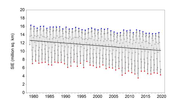
Figure 1: Arctic Sea Ice Extent ($SIE$) and Fitted Linear Trend

Notes: We show monthly average Arctic sea ice extent ($SIE$) from November 1978 to October 2019 with a fitted linear trend. Each monthly observation is a dot, and September and March observations are colored red and blue, respectively.

Figure 1 plots the time series of Arctic $SIE$ – each monthly average observation is a dot – with an overall estimated linear trend superimposed. The clear downward trend is accompanied by obvious seasonality. A more subtle feature is the possible time variation in the seasonal effects, which may be trending at different rates and possibly nonlinearly. These effects turn out to be of interest in a complete statistical representation of sea-ice dynamics.

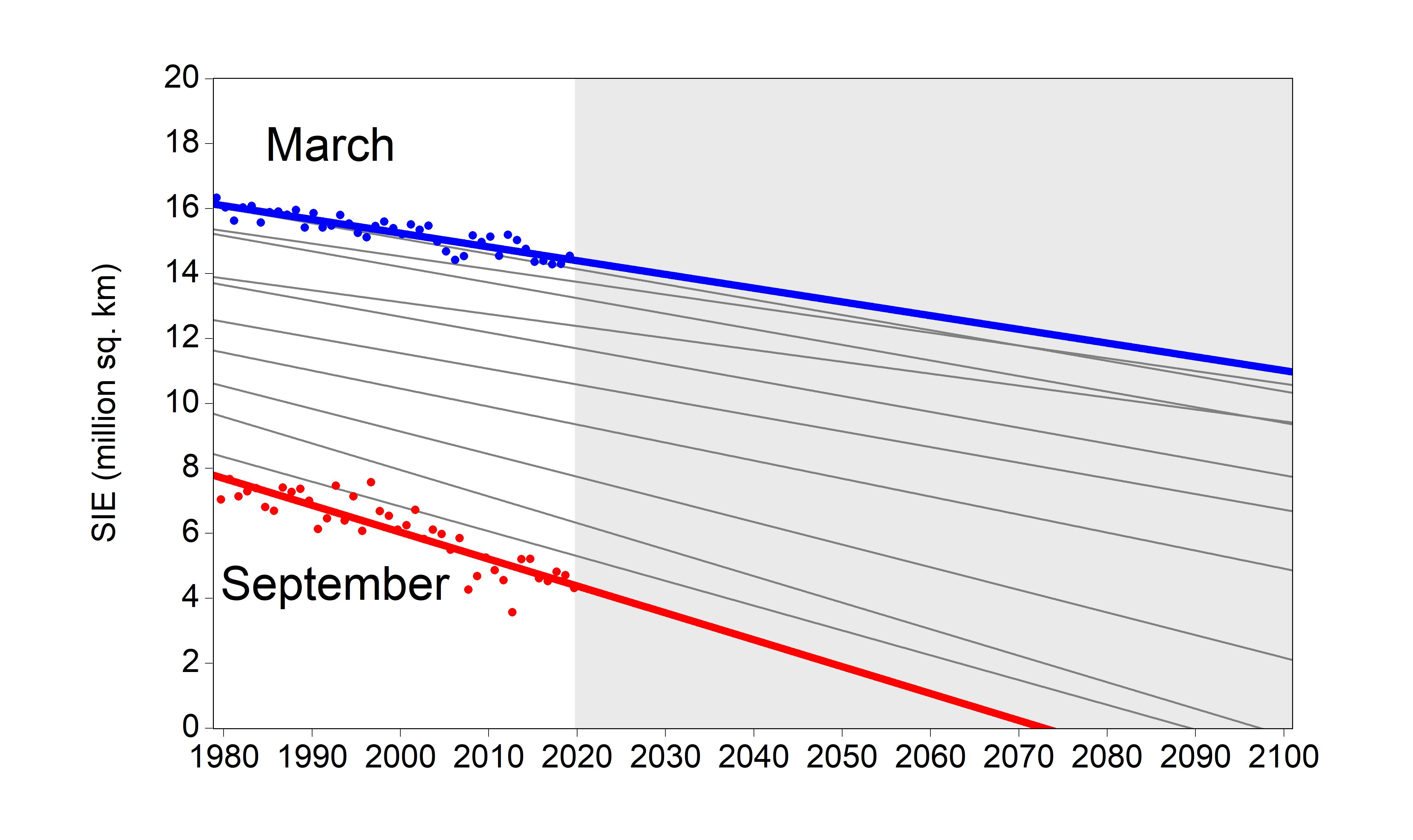
Figure 2: $SIE$: Linear Model Fits and Point Forecasts

Notes: The lines are the twelve in-sample fitted trends and out-of-sample extrapolations for Arctic $SIE$ in each month based on the linear model (1). The trends for the months with maximal and minimal sea ice extent are colored – March in blue and September in red – and the blue and red dots are the March and September historical $SIE$ data. The out-of-sample period is shaded gray.

A simple initial representation to capture this variation is a linear statistical model with twelve intercepts, one for each month, each of which may be differently trending, and potentially serially correlated stochastic shocks:

$$SIE_{t}=\sum_{i=1}^{12}\delta_{i}D_{it}+\sum_{j=1}^{12}\gamma_{j}D_{it}{\cdot}TIME_{t}+\varepsilon_{t}$$ (1)

$$\varepsilon_{t}=\rho\varepsilon_{t-1}+v_{t}$$

$$v_{t}\sim iid(0,\sigma^{2}),$$

where the $D_{i}$’s are monthly dummy variables ($D_{it}{=}1$ in month $i$ and 0 otherwise, $i{=}1,...,12$) and $TIME$ is a time dummy ($TIME_{t}{=}t$).^, We estimate model (1) – and other versions below – by maximizing the Gaussian likelihood. Detailed regression results for model (1) are in column (6) of Table A1 in Appendix A.

Figure 2 shows the resulting linear trends for all twelve months, highlighting March in blue and September in red. All of the monthly trends slope downward – an indication of a warming climate – and are highly significant. The slopes of the linear trends also differ across months (Serreze and Meier, 2019; Cavalieri and Parkinson, 2012). In particular, the seasonally low-ice months of July through October have notably steeper downward sloping trends than the seasonally high-ice months of December through May. The estimated September trend, for example, is twice as steep as the March trend, and the difference is highly statistically significant. These linear trends are also extrapolated out of sample (shaded gray) through the end of the century. For example, September sea ice extent is projected to reach zero just after 2072.

Such linear point forecasts are a useful first step, but they can be improved by allowing for nonlinearity in the trends and by quantifying forecast uncertainty – as described in section 4. First, however, we elucidate a “shadow ice” modeling approach that takes into account the fact that the measured amount of sea ice is bounded below by zero.

3 A Shadow Ice Interpretation

One consideration for downward trending statistical models for Arctic sea ice is that the measured amount of sea ice will always be non-negative. By contrast, extrapolations of simple trend models will eventually push into negative territory. There are various functional forms that can be used to model such bounded time series, and the appropriate representation depends very much on the details of the real-world phenomenon under examination. Some bounds act like reflecting barriers, so the variable of interest spends very little time at the constraint. Other bounds are absorbing states, and once reached, they may be sustained for some time.

With positive amounts of sea ice, fluctuations in SIE can serve as a rough approximation for changes in the amount of thermal energy in the Arctic; that is, hotter and colder ocean surface temperatures are reflected in less or more ice, respectively. However, this connection breaks down when the ice disappears: While SIE is fixed at zero, the surface temperature of the Arctic ocean can continue to warm. Furthermore, the warmer the ocean becomes, the less likely there will be a quick return of sea ice, which is indicative of a partially-absorbing state.

To account for this effect, the negative values of sea ice produced by a statistical model can be viewed as a rough expression of ocean temperature. Thus, we redefine the left-hand side variable of the unconstrained model as a shadow surface ice extent, $SIE^{*}$. We view $SIE^{*}$ as a notional variable that equals measured surface ice when positive, but that may also go negative to represent further increases in ocean thermal energy more broadly. Formally, to translate negative model-based sea ice values into nonnegative sea ice observations, our shadow ice model modifies the unconstrained model (1) to respect the zero lower bound for ice:

$$SIE^{*}_{t}=\sum_{i=1}^{12}\delta_{i}D_{it}+\sum_{j=1}^{12}\gamma_{j}D_{jt}{\cdot}TIME_{t}+\varepsilon_{t}$$ (2)

$$\varepsilon_{t}=\rho\varepsilon_{t-1}+v_{t}$$

$$v_{t}\sim iid(0,\sigma^{2})$$

$$SIE_{t}=\max(SIE^{*}_{t},0).$$

That is, we now interpret our earlier unconstrained linear model of surface ice as a model of shadow ice, $SIE^{*}$, so that the observed extent of sea ice, SIE, is the maximum of $SIE^{*}$ and zero.

The shadow ice model respects the nonlinearity of observed ice at the zero lower bound but retains tractability. It also allows us to translate the long-range forecasts from downward trending models like model (1) – including distributional projections – into observed data that are always non-negative. As a matter of physical interpretation, very negative values of shadow ice extent, $SIE^{*}$, represent environments in which the thermal content of the Arctic ocean is high enough that an immediate return to a positive SIE is unlikely. This shadow ice structure provides an intuitive and simple approximation of the thermodynamics of the Arctic ocean transition between sea ice and open water and serves as a useful modeling tool for observed SIE dynamics.

4 A Quadratic Statistical Model and Interval Forecasts

A downward linear trend is a common representation of the secular decline in Arctic sea ice, but linearity is not assured by the physical science. There are a variety of climate feedback mechanisms that could hasten or retard the pace of sea ice loss. The well-known ice albedo effect occurs as sea ice cover is reduced, and the resulting darker ocean surface absorbs more energy, which in turn further reduces sea ice (Stroeve et al., 2012b). This feedback effect amplifies sea ice seasonality and may progressively steepen the downward trend in $SIE$ over time (Schroeder et al., 2014). The geography of the perimeter of the Arctic Ocean, which is partially constrained by land that blocks expanding winter ice, becomes less relevant as sea ice shrinks, and relaxing this constraint may allow greater seasonal variation and a steeper downward sea ice trend (Serreze and Meier, 2019). However, there are offsetting negative feedback mechanisms – associated, for example, with increased cloud cover – that could slow the rate of sea ice loss over time (Portner et al., 2019). Indeed, Stroeve and Notz (2015) argue against trend amplification in favor of trend constancy (linearity) or trend attenuation. Moreover, as described in the next section, long-range $SIE$ projections from large-scale global climate models appear dominated by feedback mechanisms that slow the rate of September sea ice loss over time.

The lack of a complete understanding of the drivers of Arctic sea ice recommends consideration of a flexible empirical $SIE$ specification, so we generalize from linear to quadratic trends:

$$SIE^{*}_{t}=\sum_{i=1}^{12}\delta_{i}D_{it}+\sum_{j=1}^{12}\gamma_{j}D_{jt}{\cdot}TIME_{t}+\sum_{k=1}^{12}\alpha_{k}D_{kt}{\cdot}TIME_{t}^{2}+\varepsilon_{t}$$ (3)

$$\varepsilon_{t}=\rho\varepsilon_{t-1}+v_{t}$$

$$v_{t}\sim iid(0,\sigma^{2})$$

$$SIE_{t}=\max(SIE^{*}_{t},0).$$

We label model (3) as the “general” quadratic model as no constraints are imposed on the twelve quadratic ($\alpha_{k}$) parameters. The linear model (2) of course emerges under the constraint $\alpha_{1}{=}...{=}\alpha_{12}{=}0$.

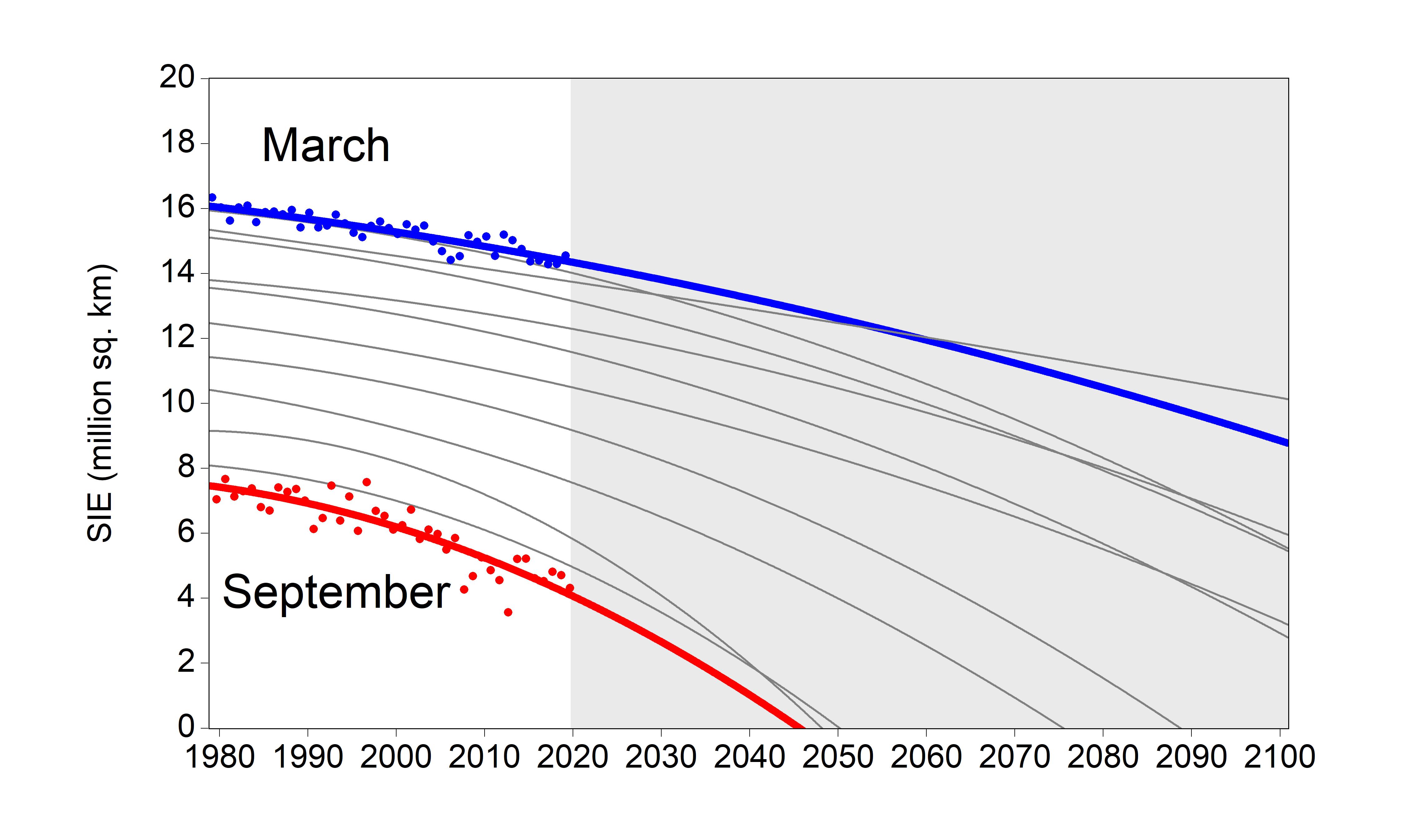
Figure 3: $SIE$: General Quadratic Model Fits and Point Forecasts

Notes: The curves are the twelve in-sample fitted trends and out-of-sample forecasts for Arctic $SIE$ in each month from the general quadratic model (3). The months with maximal and minimal sea ice extent are colored – March in blue and September in red – and the blue and red dots are the March and September historical $SIE$ data. The out-of-sample period is shaded gray.

Figure 3 shows the $SIE$ estimation fits and forecasts from the general quadratic model, by month, with March and September again highlighted in blue and red, respectively. The trend curvatures for all months are strikingly similar: the trends for all months decrease at an increasing rate. That is, the estimated $\alpha_{k}$ coefficients are negative for every month, indicating that $SIE$ is diminishing at an increasing rate. (Detailed estimation results of model (3) appear in column (1) of Table A1 in Appendix A.) The size of the estimated negative coefficients on the quadratic trend terms and their statistical significance vary by month. The most negative and significant $\alpha_{k}$ coefficients are in the seasonally low-ice “summer” months of August, September, and October, and these months show the greatest trend rates of decline. An $F$ test of the joint hypothesis that $\alpha_{8}{=}\alpha_{9}{=}\alpha_{10}{=}0$ produces a $p$-value of 0.00. Relative to a linear trend model, the nonlinear trend model forecasts lower sea ice at long horizons. February-April $SIE$ point forecasts nevertheless remain well above zero through the century, but August-October point forecasts approach zero much more quickly. Indeed the quadratic September point forecast hits zero in 2045.

Table 1 summarizes the results from investigation of the summer and non-summer differences in quadratic trend curvature using two standard model selection criteria: the Akaike information criterion (AIC) and the Bayesian information criterion (BIC). The AIC and BIC are estimates of out-of-sample forecasting performance (mean-squared error), formed by penalizing estimates of in-sample forecasting performance for degrees of freedom used in model fitting and differing only in the precise penalty applied (Diebold, 2007). The table reports these model selection criteria for six versions of the quadratic trend model (3) with various equality constraints imposed on the quadratic coefficients $\alpha_{1},...,\alpha_{12}$. Corresponding estimation results appear in Table A1 in Appendix A.

The models favored by AIC and BIC – that is, those with smaller values – are very similar and involve summer and non-summer restrictions. The AIC selects a model with equal $\alpha_{k}$’s for the nine non-summer months (November-July) and unconstrained $\alpha_{k}$’s for the three summer months (August-October). The BIC, which penalizes degrees of freedom more harshly, selects a slightly more constrained model, with the non-summer $\alpha_{k}$’s again constrained to be equal and the three summer $\alpha_{k}$’s also constrained to be equal. Compared to the unconstrained version of equation (3) – the general model – both the AIC and BIC prefer specifications with some summer and non-summer equality constraints imposed, because their imposition saves degrees of freedom without substantially degrading fit. All told, the results of Table 1 suggest a “simplified” quadratic model, namely model (3) with both summer and non-summer quadratic coefficients constrained separately to equality: $\alpha_{8}{=}\alpha_{9}{=}\alpha_{10}$ and $\alpha_{11}{=}\alpha_{12}{=}\alpha_{1}{=}...{=}\alpha_{7}$. The regression diagnostics reported in Appendix A suggest good performance of the simplified quadratic model: $R^{2}$ is almost perfect; the residual graph and Durbin-Watson statistic (DW) are consistent with random noise; and residual skewness, kurtosis, and density estimates are consistent with normality. All told, the model appears to do a fine job of capturing $SIE$ signal, reducing its complicated dynamics to Gaussian white noise.

Table 1: Akaike and Bayes Information Criteria for Quadratic Coefficient Constraints

	(1)	(2)	(3)	(4)	(5)	(6)
	NONE	Seq	NSeq	Seq+NSeq	ALLeq	ALL0
AIC	-0.0673 [3]	-0.0651 [4]	-0.0913 [1]	-0.0877 [2]	-0.0639 [5]	-0.0569 [6]
BIC	-0.2569 [6]	-0.2421 [5]	-0.1647 [2]	-0.1513 [1]	-0.1665 [4]	-0.1649 [3]

Notes: We show AIC and BIC values for the quadratic model with various equality constraints imposed on the quadratic coefficients $\alpha_{1},...,\alpha_{12}$. “NONE” denotes no constraints, which corresponds to the general quadratic model (3). “Seq” (“Summer equal”) denotes August-October equal ($\alpha_{8}{=}\alpha_{9}{=}\alpha_{10}$). “NSeq” (“Non-Summer equal”) denotes November-July equal ($\alpha_{11}{=}\alpha_{12}{=}\alpha_{1}{=}...{=}\alpha_{7}$). “Seq+NSeq” denotes summer months equal and non-summer months (separately) equal, which corresponds to the simplified quadratic model. “ALLeq ” denotes all months equal ($\alpha_{1}{=}...{=}\alpha_{12}$). “ALL0” denotes all months 0 ($\alpha_{1}{=}...{=}\alpha_{12}{=}0$), which corresponds to the linear model (1). Model ranks appear in brackets, where [1] denotes the best (smallest) criterion value. We show in boldface the best two models according to each criterion.

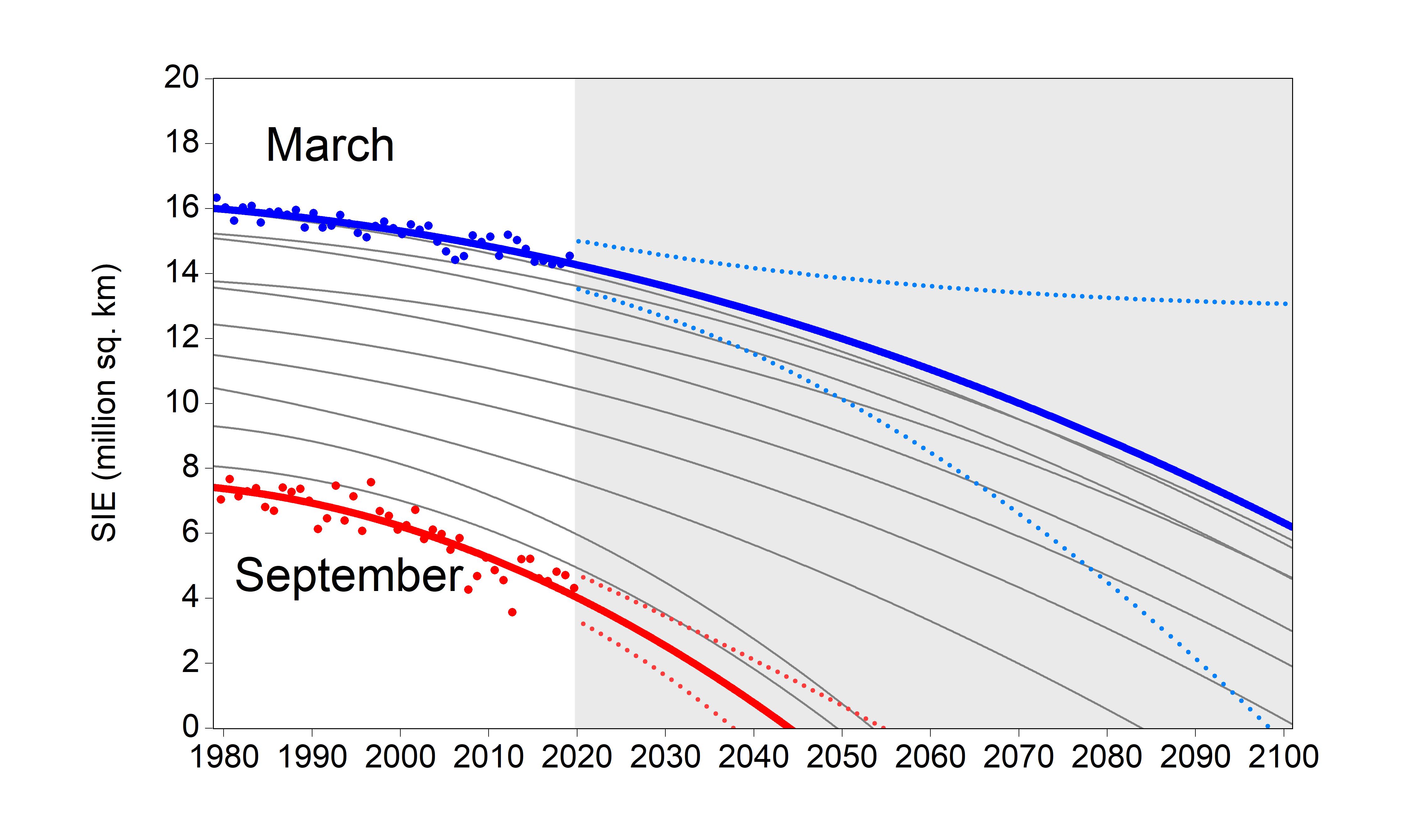
Figure 4: $SIE$: Simplified Quadratic Model Fits, Point Forecasts, and Interval Forecasts

Notes: The curves are the twelve in-sample fitted trends and out-of-sample forecasts for Arctic $SIE$ in each month from the simplified quadratic model. The months with maximal and minimal sea ice extent are colored – March in blue and September in red – and the blue and red dots are the March and September historical $SIE$ data. The out-of-sample period is shaded gray. The March and September forecasts also have $\pm\,2\,s.e.$ blue and red dotted bands that account for parameter estimation uncertainty and intrinsic uncertainty error.

Figure 4 shows the simplified quadratic model fits and forecasts. The simplified model point forecasts are very similar to those of the general quadratic model in Figure 3, with a zero-ice September also reached in 2045, but the rank ordering of the months in terms of $SIE$ is better preserved going forward. Going beyond these point forecasts, an important advantage of a formal statistical approach is that it can quantify the amount of future uncertainty. Figure 4 supplements the simplified quadratic trend point forecasts with interval or probability density forecasts. When making long-horizon interval forecasts, it is crucial to account for parameter estimation error, because its deleterious effects grow with the forecast horizon. For example, although parameter estimation error may have small effects on 6-month-ahead intervals, it will be greatly compounded for 600-month-ahead intervals. An estimate of the time-$t$ standard deviation of the forecast error, which accounts for parameter estimation error, is $\delta_{t}{=}s\sqrt{1+x_{t}^{\prime}(X^{\prime}X)^{-1}x_{t}}$, where $s$ is the standard error of the regression, $x_{t}$ is a 36$\times$1 column vector of time-$t$ right-hand-side variables, $X$ is a $T$$\times$36 matrix whose columns contain the regression’s right-hand-side variables over time, and $T$ is sample size. We use $\delta_{t}$ to produce the $\pm\,2\,\delta_{t}$ pointwise prediction intervals of Figure 4. Under normality of the shocks underlying the simplified quadratic model, the $\pm\,2\,\delta_{t}$ intervals are approximate 95 percent confidence intervals. The intervals widen rapidly; indeed the September interval starts to include zero before 2040.

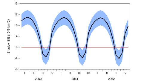
Figure 5: $SIE^{*}$: Simplified Quadratic Model Point and Interval Forecasts

Notes: We show the forecast of Arctic shadow sea ice extent, $SIE^{*}$, for 2060-2062, based on the simplified quadratic model. The solid black line is the point forecast, the shaded area is the $\pm\,2\,s.e.$ band, and the red line denotes zero.

Finally, in Figure 5 we zoom in on the 2060-2062 (36-month) segment of the simplified quadratic model shadow ice forecast. The point forecast trends down and is seasonally below zero by then. (Indeed, as already discussed, the point forecast is seasonally below zero well before then.) Moreover, the $\pm\,2\,s.e.$ intervals widen over time, and entire intervals are seasonally below zero by then. Hence it appears that, with near certainty, summer $SIE$ will vanish by 2060. This result is also clear from our earlier Figure 4, but Figure 5 highlights it in a different and complementary way.

5 Statistical versus Climate Model Projections

Of the many analyses of the long-term future evolution of Arctic ice, most have focused on projections from large-scale climate models. Such models are based on the underlying physical, chemical, and biological processes that govern the dynamics of weather and climate across ocean, air, ice, and land. The models fit an immense number of variables at a high temporal frequency and a granular spatial scale (e.g., a 30-minute time interval. a 100km worldwide horizontal resolution, and 40 vertical levels in the oceans and atmosphere). Dozens of scientific groups around the world have constructed and currently maintain such models. Occasionally, these groups conduct concurrent simulations as part of the Coupled Model Intercomparison Project (CMIP) that involve common sets of inputs including carbon emissions scenarios. The most recently completed iteration or phase of this project is the fifth one, denoted CMIP5 (Taylor et al., 2012). The CMIP5 model comparison study was the main source of climate projections included by the International Panel on Climate Change (IPCC) in its landmark Fifth Assessment Report.

Arctic $SIE$ is a key variable projected by climate models, and the models included in CMIP5 are generally judged to provide a better fit to Arctic sea ice than earlier CMIP iterations. Figure 6 shows three projections for September $SIE$ constructed as averages across sets of CMIP5 global climate models. These multi-model mean projections are constructed under three different scenarios, or Representative Concentration Pathways (RCPs), for future greenhouse gas concentrations. The brown, yellow, and blue lines are averages of the climate models, respectively, under a high level of carbon emissions (RCP8.5), a medium level (RCP6.0, yellow), and a low level (RCP4.5, blue). The first two higher emissions scenarios are viewed as more likely business-as-usual outcomes and are the most relevant to compare to statistical projections that extend the historical sample of past data and assume a continuation of the world economy’s current population and development trajectories.

The solid red line in Figure 6 shows the September trend from the simplified quadratic model estimated on the full sample from November 1978 to October 2019. The dotted lines bracketing this forecast provide an approximate 95 percent confidence interval. However, the CMIP5 climate model projections are only based on data through 2005 and do not include the past dozen or so years of sea ice observations. For comparability to these climate model projections, we re-estimated the simplified quadratic model using data from 1978 through 2005, and the September trend from this pre-2006 model is shown as the dashed red line. An interesting first result is that from the close conjunction of the two simplified model statistical projections (the solid and dashed red lines), the addition of data from 2006 to 2019 does not lead to a significant revision in the statistical trend model. The very modest differences between the pre-2006 estimated quadratic trend and the full-sample version is an indication of the stability and suitability of the simplified statistical model.

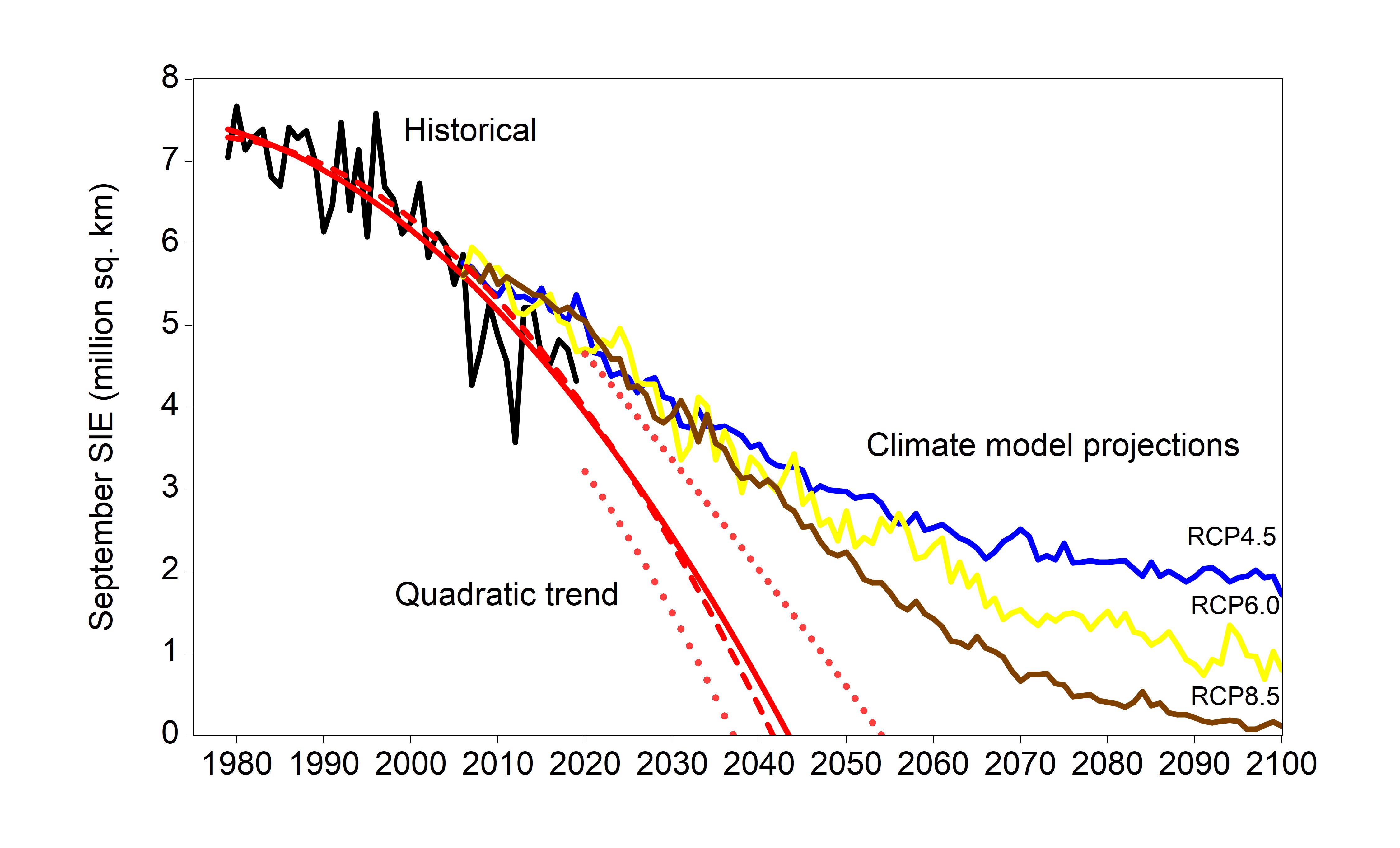
Figure 6: September $SIE$: Statistical and Climate Model Fits, Point Forecasts, and Interval Forecasts

Notes: We show fitted values and forecasts of Arctic sea ice extent, $SIE$. The solid black line is the historical data for September Arctic sea ice extent from 1979 to 2019. Mean projections from CMIP5 climate models are shown assuming underlying pathways of a high level of emissions (RCP8.5, brown), medium emissions (RCP6.0, yellow), and lower emissions (RCP4.5, blue). The climate model projections start in 2006. The red dashed line is the fitted and projected simplified quadratic model estimated using data from 1979 to 2005. The red solid line is the fitted and projected simplified quadratic trend model estimated using the full sample from 1979 to 2019, and the red dotted lines are $\pm\,2\,s.e.$ intervals (approximate 95% confidence intervals) around that projection accounting for parameter estimation uncertainty and intrinsic uncertainty.

Comparing the statistical and climate model projections in Figure 6 reveals two salient features. First, throughout the forecast period, the full-sample statistical model projection is significantly lower than any of the climate multi-model mean projections. Indeed, the climate model mean projections are well outside the 95 percent confidence intervals. Relative to the statistical model estimated on data before 2006 or the full-sample version, the climate model means are overestimating the 2019 $SIE$ trend by about 1.0 million km². This wedge is projected to increase dramatically over the next two decades. Indeed, the pre-2006 and full-sample statistical trend models project zero ice in 2042 and 2044, respectively, but none of the climate model mean projections reach a completely ice-free Arctic in this century. Notably, even assuming a high level of emissions (RCP8.5) – which is a scenario with continuing increases in average global surface temperatures throughout this century – the multi-model mean projection never reaches zero Arctic summer sea ice.

Second, in contrast to the statistical projection, the climate model mean projections show a decreasing rate of ice loss over time – that is, a concave rather than convex structure. Specifically, the climate model projections all display a roughly linear decline for the first couple of forecast decades (through around 2040) and then start to level out. For the lower emissions RCP4.5 scenario, the leveling out and deceleration of sea ice partly reflects a slowdown in the pace of global temperature increases. This effect is not at work in the RCP8.5 scenario, which has global temperatures steadily climbing through 2100. However, very close to zero sea ice extent, the leveling out of $SIE$ in RCP8.5 appears to reflect the hypothesized difficulty of melting the thick sea ice clinging near northern coastlines – notably in Greenland and Canada. Climate models generally assume that these coastal regions will retain landfast sea ice for a time even after the open Arctic Sea is free of ice. Therefore, a common definition of “ice-free” or “nearly ice-free” in the literature is a threshold of 1.0 million km² rather than zero SIE (Wang and Overland, 2009). Still, even with this higher threshold, the three climate model mean projections only reach a nearly ice-free Arctic in 2068, 2089, and $>$2100 for successively lower emissions scenarios, respectively. By contrast, the pre-2006 statistical projection reaches the higher 1.0 million km² threshold in 2037, and the full-sample statistical model reaches that level in 2039.

Some have argued that climate models generally do well in representing the large-scale evolution of Arctic sea ice (Stroeve and Notz, 2015), but a number of studies have noted that the CMIP5 global climate models overpredicted the amount of Arctic sea ice (Massonnet et al., 2012; Stroeve et al., 2012a; Serreze and Meier, 2019). That overprediction continues, and its source is not well understood. One proposed correction to this overprediction has been to focus on the models that fit the historical $SIE$ data better according to certain metrics (Wang and Overland, 2012). However, there is no agreed upon model selection criterion. Also, Rosenblum and Eisenman (2017) discount such model selection because models with more accurate sea ice readings also tend to overpredict global temperatures, so the selected climate models may be getting sea ice loss right for the wrong reason. Finally, it should be noted that from a statistical viewpoint, focusing on a simple average forecast from many models has been shown to be a robust prediction strategy (Diebold and Shin, 2019).

In some respects, the wide differences between the statistical and climate model projections are not too surprising. In climate models, the monthly observations on total Arctic SIE are a high-level output from complex, nonlinear, granular representations of the relevant underlying science. Obtaining good SIE predictions from these models requires correctly specifying a host of detailed subsidiary processes. Such a bottom-up modeling procedure has important advantages in structural interpretation and counterfactual scenario analysis. However, in a variety of disciplines, a bottom-up procedure, which carries the possibility that small misspecifications can accumulate and affect high-level aggregates, has not been found to improve prediction relative to a top-line procedure that directly models the object of interest (Diebold, 2007). Thus, based on broad previous experience, we believe that direct statistical projections of Arctic SIE are likely to be relatively accurate.

6 Probability Assessments of an Ice-Free Arctic

An advantage of a formal statistical model is its ability to make probability density forecasts for a range of possible reduced Arctic sea ice scenarios. Of particular interest are probability assessments of an ice-free or nearly ice-free Arctic, that is, the probability that $SIE_{t}$ equals zero or is less than or equal to some threshold $\gamma$, respectively. Formally, such event probabilities can be denoted as $P(SIE_{t}{\leq}\gamma)$, which represents the probability that sea ice extent is less than or equal to $\gamma$ in month $t$. We estimate these scenario probability distributions using the simplified quadratic model and a stochastic simulation procedure that accounts for parameter estimation uncertainty and allows for potentially non-Gaussian serially correlated stochastic shocks. From a given set of simulated paths, we estimate the event probabilities of interest as the proportion of simulated paths in which the event occurs out of the total number of paths.

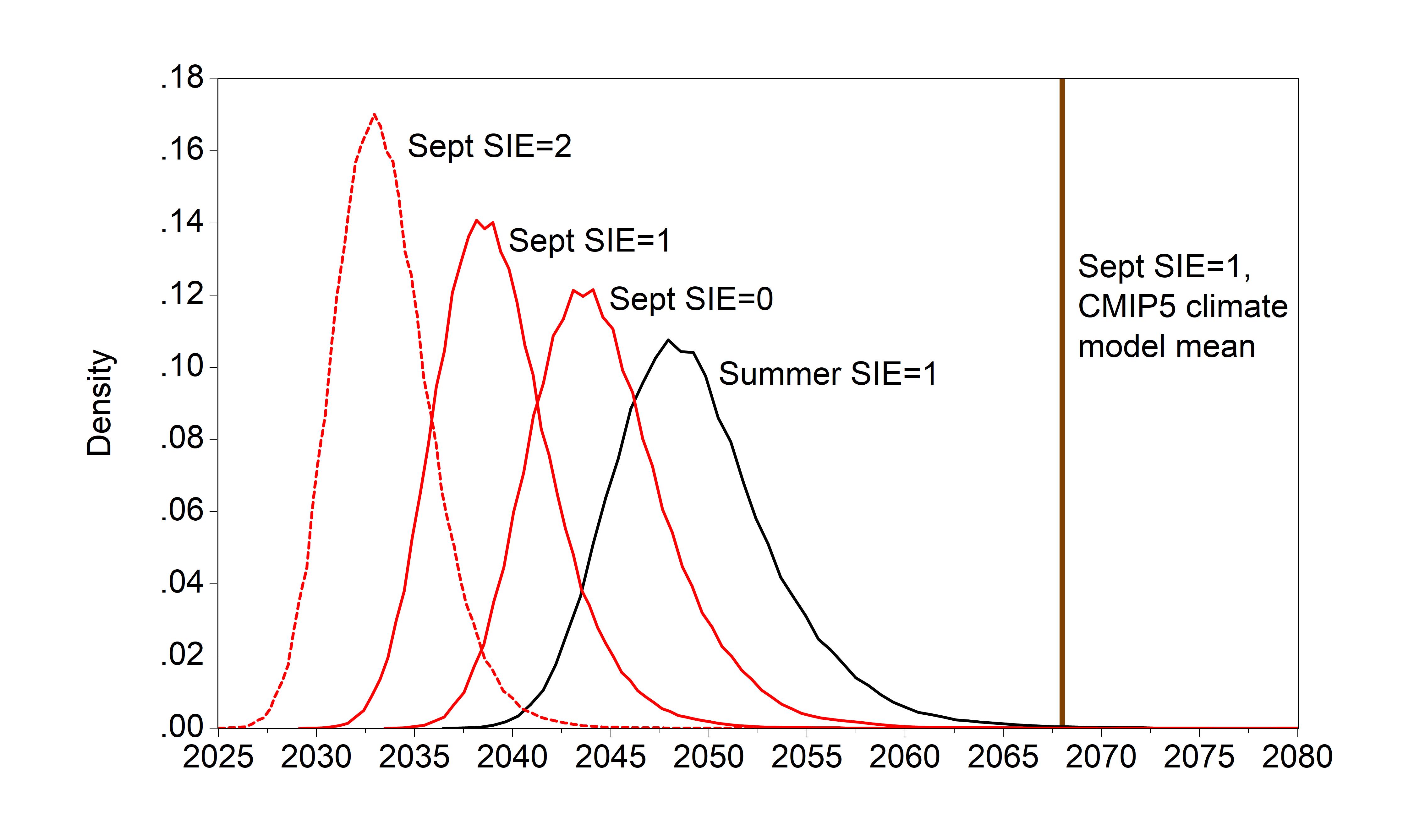
Figure 7: Probability Distributions of First Ice-Free September and First Ice-Free Summer

Notes: We display probability distributions from the simplified quadratic trend model for the date of the first effectively ice-free September (in red) and first ice-free summer (in black). The “ice-free” threshold is defined as $SIE=0$, 1, or 2 million km². The brown vertical line denotes the date that the mean CMIP5 climate model projection for RCP8.5 reaches $SIE\leq$ 1 million km².

An event that has attracted much attention in the literature is the initial occurrence of an ice-free or nearly ice-free September. We calculate the probability for each September with date $t_{0}$ so that $SIE_{t_{0}}{\leq}\gamma$ and $SIE_{t}{>}\gamma$ for all $t{<}t_{0}$. Specifically, for a given $\gamma$ and simulation $i$, we determine the year in which September $SIE_{t}$ first reaches $\gamma$, and then we cumulate across all simulations to build a distributional estimate. The red lines in Figure 7 provide the resulting probability distributions for an initial “ice-free” Arctic September for $\gamma{=}0$, $\gamma{=}1$, and $\gamma{=}2$, that is, for progressively more lenient definitions of “ice-free.” As noted above, the middle value of $\gamma$, which represents Arctic sea ice of less than $1$ million ${\rm km}^{2}$, is a popular benchmark in the literature (Wang and Overland, 2012). For that particular threshold, the statistical model produces a distribution centered at 2039. Of particular interest is the probability distribution of dates taking into account model parameter uncertainty and stochastic shock uncertainty, and this distribution shows about a 60 percent probability of an effectively ice-free September Arctic occurring in the 2030s.

The distribution with $\gamma{=}1$ is bracketed on either side by distributions that use the higher and lower thresholds. The $\gamma{=}0$ distribution has a median date of 2044 and a 95 percent range from 2039 to 2053. The $\gamma{=}2$ distribution has a median date of 2033 and an earlier and slightly narrower 95 percent range from 20230 to 2039. The climate modeling literature has pointed to several factors that underpin the uncertainty in the timing of an initial September ice-free Arctic including natural climate variability, emissions path uncertainty, and uncertain sea ice dynamics (Serreze and Meier, 2019). These factors are at least partially accounted for in our analysis.

The multi-model mean CMIP5 climate projections described above are well outside the above-described distributional ranges. For a threshold of 1 million km², the mean projections reach a nearly ice-free Arctic in 2068 and 2089 under the RCP8.5 and RCP6.0 scenarios, respectively. The former date is denoted by a vertical brown bar in Figure 7. The range of dates across individual models is also extremely wide, stretching well over a century (Jahn et al., 2016). To narrow this range, researchers have omitted models with poor performance using a variety of sea ice metrics. With such model selection procedures, the range of dates for a first nearly ice-free September is narrowed greatly to a 20-year span that runs from the 2040s to 2060s (Massonnet et al., 2012; Thackeray and Hall, 2019). Even such a carefully circumscribed span is roughly a decade later than the simplified quadratic trend model produces. Moreover, the climate model simulation exercises are not designed to yield formal error estimates or measures of uncertainty as the spread of climate model forecasts in an ensemble is insufficient to completely characterize forecast uncertainty.

Finally, we note the availability of density forecasts for a variety of richer joint scenarios of interest. As one example, Jahn et al. (2016) describe other definitions of “ice-free” that involve, for example, 5-year running means. Alternatively, “ice-free” may require no ice for several consecutive months, for example, to accommodate meaningful freight shipping, tourism, mining, and commercial fishing (Yevgeny et al., 2017). For example, the strong Autumn demand for international freight shipping to satisfy year-end Western holiday consumer demand could make a multi-month ice-free Arctic shipping lane of interest. In this case, the probability distribution of the initial occurrence of an “ice-free” summer – a joint ice-free August, September, and October – could be relevant. Figure 7 shows this distribution in black assuming an ice-free threshold of $\gamma{=}1$. This density is notably shifted right – and more right-skewed – compared to the September scenarios.

7 Concluding Remarks

A rapidly warming Arctic is an ominous sign of the broader climate change caused by human activity, but declining Arctic sea ice also has an important influence on the pace and intensity of future climate change. Using statistical models, we have provided probabilistic projections of 21st-century Arctic sea ice that account for both intrinsic uncertainty and parameter estimation uncertainty. These projections indicate that summertime Arctic sea ice will quickly diminish and disappear – with about a 60 percent probability of an effectively ice-free September Arctic occurring within two decades.

By contrast, the average projection from leading climate models implies an initial seasonal ice-free Arctic several decades later – even assuming a business-as-usual emissions path. The slow and decreasing pace at which large-scale climate models reach an ice-free Arctic may be a serious shortcoming, and such conservative projections of sea ice loss could be a misleading guide for global climate policy.

There are numerous examples, across many disciplines, showing that parsimonious statistical representations can provide forecasts that are at least as accurate as the ones from detailed structural models. However, rather than treat statistical models as just forecast competitors to structural climate models, there is likely to be scope to use them as complementary representations going forward. The mechanisms governing Arctic sea ice loss and connecting that loss to atmospheric, oceanic, and permafrost responses are not fully captured in climate models. Statistical models may be able to help assist in bridging such gaps until a more complete understanding is available (Parkinson, 2010).

In addition, statistical models may also be able to provide a benchmark for model performance that can be used for climate model evaluation, estimation/calibration, and selection. In particular, our statistical approach summarizes a key aspect of the data, namely its historical dynamics and the associated forecast path (call it $PATH_{D}$, where $D$ stands for “Data”). A climate model with calibrated parameters $\theta$ produces a corresponding summary for the model (call it $PATH_{M}(\theta)$, where $M$ stands for “Model”). So, at least conceptually, we can consider

1. evaluating a climate model by examining a measure of divergence, $||PATH_{D}{-}PATH_{M}(\theta)||$

2. estimating a climate model by finding $\hat{\theta}=argmin_{\theta}\,||PATH_{D}{-}PATH_{M}(\theta)||$ (this is precisely indirect inference (Gourieroux et al., 1993), using $PATH$ as the estimation window)

3. selecting a climate model by finding the model with smallest $||PATH_{D}{-}PATH_{M}(\hat{\theta})||$, adjusted for d.f.

In practice such formal procedures are infeasible for massive global climate models, which attempt to address all aspects of the high-dimensional climate state, of which sea ice is but one small part. Hence, for example, the “right” window for complete climate model estimation by indirect inference is much more complicated than just a sea ice path. Less formal procedures directly motivated by the above considerations can nevertheless be highly revealing, as in our key Figure 6.

Appendix A Detailed Regression Estimation Results

empty

Table A1: Regression Estimation Results, Quadratic Model with Restrictions

$SIE^{*}_{t}=\sum_{i=1}^{12}\delta_{i}D_{it}+\sum_{j=1}^{12}\gamma_{j}D_{jt}{\cdot}TIME_{t}+\sum_{k=1}^{12}\alpha_{k}D_{kt}{\cdot}TIME_{t}^{2}+\varepsilon_{t}$

$\varepsilon_{t}=\rho\varepsilon_{t-1}+v_{t}$

$v_{t}\sim iid(0,\sigma^{2})$

$SIE_{t}=\max(SIE^{*}_{t},0)$

	(1)	(2)	(3)	(4)	(5)	(6)
	NONE	Seq	NSeq	Seq+NSeq	ALLeq	ALL0
$\delta_{1}$	15.1121*	15.1372*	15.0865*	15.0922*	15.0373*	15.2274*
$\delta_{2}$	15.9436*	15.9570*	15.9404*	15.9457*	15.8894*	16.0804*
$\delta_{3}$	16.0792*	16.0820*	16.0049*	16.0100*	15.9524*	16.1446*
$\delta_{4}$	15.3521*	15.3443*	15.2278*	15.2326*	15.1741*	15.3674*
$\delta_{5}$	13.8027*	13.7832*	13.7604*	13.7650*	13.7056*	13.9001*
$\delta_{6}$	12.4776*	12.4443*	12.4352*	12.4397*	12.3796*	12.5749*
$\delta_{7}$	10.4243*	10.3733*	10.4804*	10.4849*	10.4243*	10.6202*
$\delta_{8}$	8.0945*	8.0202*	8.1441*	8.0754*	8.2547*	8.4508*
$\delta_{9}$	7.4698*	7.3645*	7.5179*	7.4201*	7.6022*	7.7976*
$\delta_{10}$	9.1633*	9.2520*	9.2146*	9.3080*	9.4932*	9.6870*
$\delta_{11}$	11.4307*	11.4872*	11.4928*	11.4997*	11.4488*	11.6374*
$\delta_{12}$	13.5642*	13.6042*	13.5673*	13.5735*	13.5205*	13.7097*

Estimation Results, Quadratic Model with Restrictions (Continued)

	(1)	(2)	(3)	(4)	(5)	(6)
	NONE	Seq	NSeq	Seq+NSeq	ALLeq	ALL0
$\gamma_{1}$	-0.0026	-0.0029*	-0.0023	-0.0024*	-0.0017	-0.0040*
$\gamma_{2}$	-0.0023	-0.0024	-0.0022*	-0.0023*	-0.0016	-0.0039*
$\gamma_{3}$	-0.0027	-0.0028	-0.0018*	-0.0019	-0.0012	-0.0035*
$\gamma_{4}$	-0.0031	-0.0030	-0.0016	-0.0016	-0.0009	-0.0033*
$\gamma_{5}$	-0.0019	-0.0016	-0.0014	-0.0014	-0.0007	-0.0031*
$\gamma_{6}$	-0.0028	-0.0024	-0.0023*	-0.0024*	-0.0016	-0.0040*
$\gamma_{7}$	-0.0034*	-0.0028*	-0.0041*	-0.0042*	-0.0034*	-0.0058*
$\gamma_{8}$	-0.0021	-0.0012	-0.0027	-0.0019	-0.0040*	-0.0064*
$\gamma_{9}$	-0.0030*	-0.0018	-0.0036*	-0.0024*	-0.0045*	-0.0069*
$\gamma_{10}$	-0.0006	-0.0016	-0.0012	-0.0023*	-0.0044*	-0.0068*
$\gamma_{11}$	-0.0021	-0.0028*	-0.0029*	-0.0030*	-0.0023*	-0.0046*
$\gamma_{12}$	-0.0023	-0.0028	-0.0024*	-0.0024*	-0.0017	-0.0041*
$\alpha_{1}$	-2.72E-06	-2.11E-06	-3.40E-06	-3.29E-06	-4.78E-06*	0
$\alpha_{2}$	-3.31E-06	-2.99E-06	-3.40E-06	-3.29E-06	-4.78E-06*	0
$\alpha_{3}$	-1.53E-06	-1.47E-06	-3.40E-06	-3.29E-06	-4.78E-06*	0
$\alpha_{4}$	-3.24E-07	-5.17E-06	-3.40E-06	-3.29E-06	-4.78E-06*	0
$\alpha_{5}$	-2.38E-06	-2.84E-06	-3.40E-06	-3.29E-06	-4.78E-06*	0
$\alpha_{6}$	-2.39E-06	-3.18E-06	-3.40E-06	-3.29E-06	-4.78E-06*	0
$\alpha_{7}$	-4.78E-06	-5.96E-06*	-3.40E-06	-3.29E-06	-4.78E-06*	0
$\alpha_{8}$	-8.57E-06*	-1.03E-05*	-7.35E-06*	-8.96E-06*	-4.78E-06*	0
$\alpha_{9}$	-7.89E-06*	-1.03E-05*	-6.69E-06*	-8.96E-06*	-4.78E-06*	0
$\alpha_{10}$	-1.24E-05*	-1.03E-05*	-1.11E-05*	-8.96E-06*	-4.78E-06*	0
$\alpha_{11}$	-4.99E-06*	-3.57E-06	-3.40E-06	-3.29E-06	-4.78E-06*	0
$\alpha_{12}$	-3.45E-06	-2.48E-06	-3.40E-06	-3.29E-06	-4.78E-06*	0
$\rho$	0.7302*	0.7284*	0.7298*	0.7270*	0.7288*	0.7461*
$\sigma^{2}$	0.0468*	0.0473*	0.0472*	0.0478*	0.0491*	0.0497*
$R^{2}$	0.996	0.995	0.995	0.995	0.995	0.995
$DW$	1.71	1.71	1.71	1.71	1.71	1.72
$Skew$	-0.17	-0.19	-0.16	-0.20	-0.18	-0.14
$Kurt$	3.77	3.75	3.70	3.70	3.93	3.95

Estimation Results, Quadratic Model with Restrictions (Continued)

Notes to table: We show maximum-likelihood estimates of the parameters of the general quadratic model (3), with various equality constraints imposed on the quadratic coefficients $\alpha_{1},...,\alpha_{12}$. “NONE” denotes no constraints, which corresponds to the general quadratic model (3). “Seq” (“Summer equal”) denotes August-October equal ($\alpha_{8}{=}\alpha_{9}{=}\alpha_{10}$). “NSeq” (“Non-Summer equal”) denotes November-July equal ($\alpha_{11}{=}\alpha_{12}{=}\alpha_{1}{=}...{=}\alpha_{7}$). “Seq+NSeq” denotes summer months equal and non-summer months (separately) equal, which corresponds to the simplified quadratic model. “ALLeq” denotes all months equal ($\alpha_{1}{=}...{=}\alpha_{12}$). “ALL0” denotes all months 0 ($\alpha_{1}{=}...{=}\alpha_{12}{=}0$), which corresponds to the linear model (1). In each column, we show constrained parameter estimates in boldface. “*” denotes significance at the ten percent level.

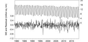
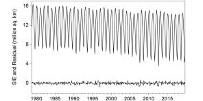
Figure A1: $SIE$, Actual and Residual

Notes: The left panel uses different scales (actual on the right, residual on the left), so the residual is greatly enlarged. The right panel uses a common scale, making clear that the residual is negligible.

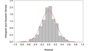
Figure A2: $SIE$ Residual Histogram and Best-Fitting Gaussian

Notes: We show the residual histogram, together with a Gaussian density fit to the residuals.

Appendix B Simulation Methods

We estimate scenario probability distributions using the simplified quadratic model (that is, the quadratic model (3) subject to the constraints $\alpha_{8}{=}\alpha_{9}{=}\alpha_{10}$ and $\alpha_{11}{=}\alpha_{12}{=}\alpha_{1}{=}...{=}\alpha_{7}$) and a simulation procedure that accounts for parameter estimation uncertainty and allows for potentially non-Gaussian serially correlated stochastic shocks. To describe this simulation procedure, it is useful to re-write the quadratic model (3) in a more concise notation:

$$SIE^{*}_{t}=x^{\prime}_{t}\beta+\varepsilon_{t}$$

$$\varepsilon_{t}=\rho\varepsilon_{t-1}+v_{t}$$

$$v_{t}\sim iid(0,\sigma^{2})$$

$$SIE_{t}=\max(SIE^{*}_{t},0),$$

where $x^{\prime}_{t}{=}(D_{1t},...,D_{12t},~{}D_{1t}{\cdot}TIME_{t},...,D_{12t}{\cdot}TIME_{t},~{}D_{1t}{\cdot}TIME_{t}^{2},...,D_{1t}{\cdot}TIME_{t}^{2})$ and

$\beta^{\prime}{=}(\delta_{1},...,\delta_{12},\gamma_{1},...,\gamma_{12},\alpha_{1},...,\alpha_{12})$. We estimate the model by maximum likelihood using the historical data sample $t=1,...,T$, as discussed earlier, and then we simulate $i=1,...,10,000$ future paths based on the estimated model. Simulation $i$ proceeds as follows:

1. Draw ${\beta}^{(i)}$ from the sampling distribution of the estimated parameter vector $\hat{\beta}$, and form $x^{\prime}_{t}{\beta}^{(i)}$, $t=T{+}1,...,2099M12$.

2. Draw $v_{t}^{(i)}$ by sampling with replacement from the observed $\hat{v}_{t}$’s (with equal weights $1/T$), $t=T{+}1,...,2099M12$.

3. Draw ${\rho}^{(i)}$ from the sampling distribution of $\hat{\rho}$, and form $\varepsilon_{t}^{(i)}={\rho}^{(i)}\varepsilon_{t-1}+v_{t}^{(i)}$, $t=T{+}1,...,2099M12$, using the last observed historical residual $\hat{\varepsilon}_{T}$ as the initial condition.

4. Form $SIE_{t}^{(i)}=x^{\prime}_{t}{\beta}^{(i)}+{\varepsilon}^{(i)}_{t}$, $t=T{+}1,...,2099M12$.

Finally, we estimate event probabilities of interest as the relative frequency of occurrence across the simulated paths.

References

- (1)
- Arthun et al. (2012) Arthun, M., T. Eldevik, L.H. Smedsrud, Ø. Skagseth, and R.B. Ingvaldsen (2012), “Quantifying the Influence of Atlantic Heat on Barents Sea Ice Variability and Retreat,” Journal of Climate, 25, 4736–4743.
- Bauer and Rudebusch (2016) Bauer, M.D. and G.D. Rudebusch (2016), “Monetary Policy Expectations at the Zero Lower Bound,” Journal of Money, Credit and Banking, 48, 1439–1465.
- Bekkers et al. (2016) Bekkers, E., J.F. Francois, and H. Rojas-Romagosa (2016), “Melting Ice Caps and the Economic Impact of Opening the Northern Sea Route,” Economic Journal, 128, 1095–1127.
- Cavalieri and Parkinson (2012) Cavalieri, D.J. and C.L. Parkinson (2012), “Arctic Sea Ice Variability and Trends, 1979-2010,” The Cryosphere, 6, 881–889.
- Christensen and Rudebusch (2014) Christensen, J.H.E. and G.D. Rudebusch (2014), “Estimating Shadow-Rate Term Structure Models with Near-Zero Yields,” Journal of Financial Econometrics, 13, 226–259.
- Diebold (2007) Diebold, F.X. (2007), Elements of Forecasting, fourth edition, South-Western.
- Diebold et al. (2020) Diebold, F.X., M. Göbel, P. Goulet Coulombe, G.D. Rudebusch, and B. Zhang (2020), “Optimal Combination of Arctic Sea Ice Extent Measures: A Dynamic Factor Modeling Approach,” International Journal of Forecasting, in press.
- Diebold and Shin (2019) Diebold, F.X. and M. Shin (2019), “Machine Learning for Regularized Survey Forecast Combination: Partially-Egalitarian Lasso and its Derivatives,” International Journal of Forecasting, 35, 1675–1691.
- Ebinger and Zambetakis (2009) Ebinger, C.K. and E. Zambetakis (2009), “The Geopolitics of Arctic Melt,” International Affairs, 85, 1215–1232.
- Fetterer et al. (2017) Fetterer, F., K. Knowles, W. Meier, M. Savoie, and A.K. Windnagel (2017), “Sea Ice Index, Version 3, Dataset ID G02135,” Boulder, Colorado, USA. NSIDC: National Snow and Ice Data Center. https://doi.org/10.7265/N5K072F8, updated daily, accessed October 2019.
- Goldstein et al. (2018) Goldstein, M.A., A.H. Lynch, A. Zsom, T. Arbetter, A. Chang, and F. Fetterer (2018), “The Step-Like Evolution of Arctic Open Water,” Scientific Reports, 8, 2045–2322.
- Gourieroux et al. (1993) Gourieroux, C., A. Monfort, and E. Renault (1993), “Indirect Inference,” Journal of Applied Econometrics, 8, S85–S118.
- Guarino et al. (2020) Guarino, M.V., L.C. Sime, D. Schroeder, I. Malmierca-Vallet, E. Rosenblum, M. Ringer, J. Ridley, D. Feltham, C. Bitz, E.J. Steig, and E. Wolff (2020), “Sea-Ice Free Arctic During the Last Interglacial Supports Fast Future Loss,” Nature Climate Change, 1–5.
- Guemas et al. (2016) Guemas, V., E. Blanchard-Wrigglesworth, M. Chevallier, J.J. Day, M. Déqué, F.J. Doblas-Reyes, N.S. Fučkar, A. Germe, E. Hawkins, S. Keeley, T. Koenigk, D. Salas y Mélia, and S. Tietsche (2016), “A Review on Arctic Sea-ice Predictability and Prediction on Seasonal to Decadal Time-scales,” Quarterly Journal of the Royal Meteorological Society, 142, 546–561.
- Hall et al. (2013) Hall, A.R., D.R. Osborn, and N. Sakkas (2013), “Inference on Structural Breaks Using Information Criteria,” The Manchester School, 81, 54–81.
- Hudson (2011) Hudson, S.R. (2011), “Estimating the Global Radiative Impact of the Sea Ice-Albedo Feedback in the Arctic,” Journal of Geophysical Research: Atmospheres, 116, D16102, doi:10.1029/2011JD015804.
- Ionita et al. (2019) Ionita, M., K. Grosfeld, P. Scholz, R. Treffeisen, and G. Lohmann (2019), “September Arctic Sea Ice Minimum Prediction – A Skillful New Statistical Approach,” Earth System Dynamics, 10, 189–203.
- Jahn et al. (2016) Jahn, A., J.E. Kay, M.M. Holland, and D.M. Hall (2016), “How Predictable is the Timing of a Summer Ice-Free Arctic?” Geophysical Research Letters, 43, 9113–9120.
- Johnston and DiNardo (1972) Johnston, J. and J. DiNardo (1972), Econometric Methods, New York.
- Kattsov et al. (2010) Kattsov, V.M., V.E. Ryabinin, J.E. Overland, M.C. Serreze, M. Visbeck, J.E. Walsh, W. Meier, and X. Zhang (2010), “Arctic Sea Ice Change: A Grand Challenge of Climate Science,” Journal of Glaciology, 56, 1115–1121.
- Liu and Fedorov (2019) Liu, W. and A.V. Fedorov (2019), “Global Impacts of Arctic Sea Ice Loss Mediated by the Atlantic Meridional Overturning Circulation,” Geophysical Research Letters, 46, 944–952.
- Massonnet et al. (2012) Massonnet, F., T. Fichefet, H. Goosse, C. Bitz, G. Philippon-Berthier, M. Holland, and P.Y. Barriat (2012), “Constraining Projections of Summer Arctic Sea Ice,” The Cryosphere, 6, 1383–1394.
- Nelson (1972) Nelson, C.R. (1972), “The Prediction Performance of the FRB-MIT-Penn Model of the U.S. Economy,” American Economic Review, 62, 902–917.
- Obryk et al. (2019) Obryk, M.K., P.T. Doran, and J.C. Priscu (2019), “Prediction of Ice-Free Conditions for a Perennially Ice-Covered Antarctic Lake,” Journal of Geophysical Research: Earth Surface, 124, 686–694.
- Ono et al. (2018) Ono, J., H. Tatebe, Y. Komuro, M. I. Nodzu, and M. Ishii (2018), “Mechanisms Influencing Seasonal to Inter-annual Prediction Skill of Sea Ice Extent in the Arctic Ocean in MIROC,” The Cryosphere, 12, 675–683.
- Osborne et al. (2018) Osborne, E., J. Richter-Menge, and M. Jeffries (2018), “Sea Ice,” https://www.arctic.noaa.gov/Report-Card, accessed: 2019-09-26.
- Parkinson (2010) Parkinson, C. L. (2010), Coming Climate Crisis?, Rowman and Littlefield, chapter 10.
- Peng et al. (2018) Peng, G., J.L. Matthews, and J.T. Yu (2018), “Sensitivity Analysis of Arctic Sea Ice Extent Trends and Statistical Projections Using Satellite Data,” Remote Sensing, 10, 230.
- Petoukhov and Semenov (2010) Petoukhov, V. and V.A. Semenov (2010), “A Link Between Reduced Barents-Kara Sea Ice and Cold Winter Extremes Over Northern Continents,” Journal of Geophysical Research: Atmospheres, 115, D21111, doi:10.1029/2009JD013568.
- Petrick et al. (2017) Petrick, S., K. Riemann-Campe, S. Hoog, C. Growitsch, H. Schwind, R. Gerdes, and K. Rehdanz (2017), “Climate Change, Future Arctic Sea Ice, and the Competitiveness of European Arctic Offshore Oil and Gas Production on World Markets,” Ambio, 46, 410–422.
- Petty et al. (2017) Petty, A.A., J.C. Stroeve, P.R. Holland, L.N. Boisvert, A.C. Bliss, N. Kimura, and W.N. Meier (2017), “The Arctic Sea Ice Cover of 2016: A Year of Record-Low Highs and Higher-Than-Expected Lows,” The Cryosphere, 12, 433–452.
- Portner et al. (2019) Portner, H.O., D.C. Roberts, V. Masson-Delmotte, P. Zhai, M. Tignor, E. Poloczanska, K. Mintenbeck, M. Nicolai, A. Okem, J. Petzold, B. Rama, and N. Weyer (2019), IPCC, 2019: IPCC Special Report on the Ocean and Cryosphere in a Changing Climate, https://www.ipcc.ch/srocc/cite-report/.
- Reidmiller et al. (2018) Reidmiller, D.R., C.W. Avery, D.R. Easterling, K.E. Kunkel, K.L.M. Lewis, T.K. Maycock, and B.C. Stewart (eds.) (2018), “USGCRP, 2018: Impacts, Risks, and Adaptation in the United States: Fourth National Climate Assessment, Volume II,” USGCRP, 2018: Impacts, Risks, and Adaptation in the United States: Fourth National Climate Assessment, Volume II, U.S. Global Change Research Program, Washington, DC, USA. doi: 10.7930/NCA4.2018, https://nca2018.globalchange.gov/chapter/front-matter-guide.
- Rocha and Cribari-Neto (2008) Rocha, A.V. and F. Cribari-Neto (2008), “Beta Autoregressive Moving Average Models,” TEST, 18, 529.
- Rosenblum and Eisenman (2017) Rosenblum, E. and I. Eisenman (2017), “Sea Ice Trends in Climate Models Only Accurate in Runs with Biased Global Warming,” Journal of Climate, 30, 6265–6278.
- Schlichtholz (2011) Schlichtholz, P. (2011), “Influence of Oceanic Heat Variability on Sea Ice Anomalies in the Nordic Seas,” Geophysical Research Letters, 38.
- Schroeder et al. (2014) Schroeder, D., D.L. Feltham, D. Flocco, and M. Tsamados (2014), “September Arctic Sea-Ice Minimum Predicted by Spring Melt-Pond Fraction,” Nature Climate Change, 4, 353–357.
- Selyuzhenok et al. (2020) Selyuzhenok, V., I. Bashmachnikov, R. Ricker, A. Vesman, and L. Bobylev (2020), “Sea Ice Volume Variability and Water Temperature in the Greenland Sea,” Cryosphere, 14.
- Serreze and Meier (2019) Serreze, M.C. and W.N. Meier (2019), “The Arctic’s Sea Ice Cover: Trends, Variability, Predictability, and Comparisons to the Antarctic,” Annals of the New York Academy of Sciences, 1436, 36–53.
- Snape and Forster (2014) Snape, T.J. and P.M. Forster (2014), “Decline of Arctic Sea Ice: Evaluation and Weighting of CMIP5 Projections,” Journal of Geophysical Research: Atmospheres, 119, 546–554.
- Stroeve et al. (2007) Stroeve, J., M.M. Holland, W. Meier, T. Scambos, and M. Serreze (2007), “Arctic Sea Ice Decline: Faster than Forecast,” Geophysical Research Letters, 34, L09501, doi: 10.1029/2007GL029703.
- Stroeve and Notz (2015) Stroeve, J. and D. Notz (2015), “Insights on Past and Future Sea-Ice Evolution from Combining Observations and Models,” Global and Planetary Change, 135, 119–132.
- Stroeve and Notz (2018) Stroeve, J. and D. Notz (2018), “Changing State of Arctic Sea Ice Across All Seasons,” Environmental Research Letters, 13.
- Stroeve et al. (2012a) Stroeve, J.C., V. Kattsov, A. Barrett, M. Serreze, T. Pavlova, M. Holland, and W.N. Meier (2012a), “Trends in Arctic Sea Ice Extent from CMIP5, CMIP3 and Observations,” Geophysical Research Letters, 39, L16502, doi:10.1029/2012GL052676.
- Stroeve et al. (2012b) Stroeve, J.C., M.C. Serreze, M.M. Holland, J.E. Kay, J. Malanik, and A.P. Barrett (2012b), “The Arctic’s Rapidly Shrinking Sea Ice Cover: A Research Synthesis,” Climatic Change, 110, 1005–1027.
- Tanski et al. (2019) Tanski, G., D. Wagner, C. Knoblauch, M. Fritz, T. Sachs, and H. Lantuit (2019), “Rapid CO2 Release from Eroding Permafrost in Seawater,” Geophysical Research Letters, 46, 11244–11252.
- Taylor et al. (2012) Taylor, K.E., R.J. Stouffer, and G.A. Meehl (2012), “An Overview of CMIP5 and the Experiment Design,” Bulletin of the American Meterological Society, 93, 485–498.
- Thackeray and Hall (2019) Thackeray, C.W. and A. Hall (2019), “An Emergent Constraint on Future Arctic Sea-Ice Albedo Feedback,” Nature Climate Change, 9, 972–978.
- Trusel et al. (2018) Trusel, L.D., S.B. Das, M.B. Osman, M.J. Evans, B.E. Smith, X. Fettweis, J.R. McConnell, B.P.Y. Noel, and M.R. Van den Broeke (2018), “Nonlinear Rise in Greenland Runoff in Response to Post-Industrial Arctic Warming,” Nature, 564, 104–108.
- Wallis (1987) Wallis, K.F. (1987), “Time Series Analysis of Bounded Economic Variables,” Journal of Time Series Analysis, 8, 115–123.
- Wang et al. (2016) Wang, L., X. Yuan, M. Ting, and C. Li (2016), “Predicting Summer Arctic Sea Ice Concentration Intraseasonal Variability Using a Vector Autoregressive Model,” Journal of Climate, 29, 1529–1543.
- Wang and Overland (2009) Wang, M. and J.E. Overland (2009), “A Sea Ice Free Summer Arctic Within 30 Years?” Geophysical Research Letters, 36, L07502, doi:10.1029/2009GL037820.
- Wang and Overland (2012) Wang, M. and J.E. Overland (2012), “A Sea Ice Free Summer Arctic Within 30 Years: An Update from CMIP5 Models,” Geophysical Research Letters, 39, L18501, doi:10.1029/2012GL052868.
- Yevgeny et al. (2017) Yevgeny, A., E.E. Popova, A. Yool, A.J.G. Nurser, T.D. Williams, Laurent B., and Jon B. (2017), “On the Future Navigability of Arctic Sea Routes: High-resolution Projections of the Arctic Ocean and Sea Ice”,” Marine Policy, 75, 300–317.