5D Light Field Synthesis from a Monocular Video

Abstract

Commercially available light field cameras have difficulty in capturing 5D (4D + time) light field videos. They can only capture still light filed images or are excessively expensive for normal users to capture the light field video. To tackle this problem, we propose a deep learning-based method for synthesizing a light field video from a monocular video. We propose a new synthetic light field video dataset that renders photorealistic scenes using UnrealCV rendering engine because no light field dataset is avaliable. The proposed deep learning framework synthesizes the light field video with a full set (9$\times$9) of sub-aperture images from a normal monocular video. The proposed network consists of three sub-networks, namely, feature extraction, 5D light field video synthesis, and temporal consistency refinement. Experimental results show that our model can successfully synthesize the light field video for synthetic and actual scenes and outperforms the previous frame-by-frame methods quantitatively and qualitatively. The synthesized light field can be used for conventional light field applications, namely, depth estimation, viewpoint change, and refocusing.

1 Introduction

The recent decade witnessed a rapid growth of light field technology which has received substantial interest in the fields of computer vision and graphics. Different from a conventional image, a light field image captures 4D light information of directional rays through the main lens of the camera instead of accumulating them. Direct applications, depth image estimation [23, 24, 33, 34], image refocusing [18], saliency detection [14], and view-point change are performed using only a single shot of light field image as a post-capturing process. Traditionally, light field images are captured using a plenoptic camera consisting of a microlens array or a multicamera array [32]. However, Lytro’s camera, which was commercially available for general users, is no longer avaliable in the market. The only available camera is Raytrix [1], which can capture light field videos. However, it is used for industrial and research purposes. Therefore, it is much expensive for general users for daily use. To overcome these limitations, various methods for synthesizing light field images from normal images, i.e. without using a light field camera, have been proposed [9, 11, 17, 26, 27, 35, 36, 42]. However, the goal is to synthesize light field still images, not videos. To the best of our knowledge, no previous work has synthesized a light field video from a normal monocular video.

(a)

(b)

(c)

Figure 1: Synthesized light field frames and their applications. The network is trained only with the synthetic dataset. (a) Synthesized light field images (center sub-aperture images and epipolar images) on synthetic and actual datasets. (b) Estimated depth. (c) Estimated appearance flow.

Conventional learning-based light field synthesis methods are inspired by depth estimation techniques [4, 5, 7, 37]. Most methods require a sparse set (4$\sim$9) of input images to synthesize a single light field image ($8\times 8\sim 10\times 10$). [27] synthesized a light field image from a single input image, but it is highly dependent on the quality of the estimated depth image. [9] also synthesized a light field image from a single input image with improved generality of object and robustness. Note that [27] and [9] can only generate a light field video using a frame-by-frame approach. Therefore, temporal consistency cannot be guaranteed.

A light field video capturing method was proposed by [28]. It uses a hybrid camera system combining a general DSLR camera and a light field camera (Lytro) and synthesizes the light field video. This method cannot be generalize to in-the-wild video capture and it is prone to error due to a viewpoint mismatch between two cameras.

Deep learning-based methods require a large-sized dataset to train the network. However, acquiring a dataset that exactly fits a specific purpose is not trivial. Especially for the light field, no video training dataset can be used for light field video processing. To overcome this limitation, similar to the approach used in [21, 40, 21, 22, 20], we use a graphics-generated photorealistic video simulated on a virtual environment. In our approach, we use UnrealCV [19] which is based on the Unreal4 game graphics engine to collect the synthetic light field video consisting of 9$\times$9 sub-aperture images (SAIs). Using synthetic light field data avoids the limitations of previous light field images, i.e. low spatial/angular resolution, and small baseline.

In this paper, we propose a novel framework for 5D light field video synthesis.We introduce a correlation layer to find correspondence between adjacent input frames and use it to estimate optical flow and appearance flow. Figure 1 shows the synthesized light field video frames and their applications for synthetic and actual scenes. As shown in Figure 1, although we trained our framework with a synthetic dataset, it performs well in synthesizing a light field video from an actual scene. The key contributions of this paper are summarized as follows:

• an end-to-end deep learning-based framework for 5D light field video synthesis.

• a new photorealistic synthetic dataset for light field video synthesis network training.

• capability of synthesizing light field video for actual images while the network is trained on the synthetic dataset.

2 Related Works

Light Field Synthesis

The light field image, first proposed by Lippmann et al. [15], was introduced in 2005 in the form of a plenoptic camera by Ng et al. [18], and its potential has since attracted attention. At the same time, an increasing demand to synthesize light field images of a large amount of SAI from a small number of images is observed. Wanner and Goldluecke [31] estimated the disparity maps using epipolar plane image (EPI) analysis of light field images and proposed super-resolution and view synthesis of light field images. Zhang et al. [41] proposed a method for synthesizing light field images using a disparity assisted phase-based light field synthesis based on the difference of stereo images with a small baseline.

A learning-based light field image synthesis method was first proposed by Kalantari et al. [11]. In this method, a network for estimating the disparity between each viewpoint and a network for correcting the color of the synthesized light field image are used to synthesize a 4D light field image using four input images located at the corners of the light field image. Wu et al. [36] synthesized the light field images from a minimum of nine and a maximum of 25 input images using an EPI super-resolution with a special blur kernel. Wang et al. [29] and Yeung et al. [35] used a 4D CNN for synthesizing light field images from a sparse set of input images.

A method for synthesizing light field image from a single image rather than multiple input images was first proposed by Srinivasan et al. [27]. In this method, a depth image corresponding to each SAI is initially estimated from an input image, and then a novel view is synthesized by warping the input image. Then, a light field image is synthesized in the angular domain through a color estimation network. However, the drawback is that the method depends heavily on the quality of the estimated depth and the color information of the image. Ivan and Park [9] synthesized the light field image using the appearance flow proposed by Zhou et al. [43] rather than the depth image. However, as with [27], the limitation is that it is unsuitable for synthesizing the light field video because it aims to synthesize the light field image of the static object.

A method for synthesizing a multiview image with a large baseline rather than a light field image has also been proposed. Huang et al. [8] proposed a method for synthesizing a horizontal light field image using multiple input images and camera pose information. Zhou et al. [42] proposed a method for synthesizing a horizontal light field image from a stereo image with a small baseline using a new scene representation called a multiplane image (MPI). However, these methods have limitations that require two or more input images or even camera parameters, which are difficult for a general user to provide. In et al. [26], [42] is extended, and a method for synthesizing light field images with a large baseline using MPI is proposed. Mildenhall et al. [17] proposed a method for synthesizing light field images with large baselines using MPI as well. Although [26] and  [17] proposed a method for synthesizing a light field image with a large baseline rather than a conventional light field image, the limitation is that a large amount of computation and two or more input images are required.

The method for synthesizing light field videos was proposed by Wang et al. [28] using a hybrid camera system consisting of a general DSLR camera and a light field camera. It acquires videos simultaneously with a light field camera (3fps) and a DSLR camera (30fps), and then the light field video is synthesized. However, this method requires not only a standard camera but also a light field camera. In addition, errors occur due to the viewpoint mismatch between the two cameras.

In this paper, we deal with the synthesis of light field images, especially the synthesis of light field videos. Different from conventional methods, no camera position information and no two or more input images are required to synthesize one light field image. We also propose a deep learning-based framework that synthesizes a light field video from a monocular video rather than a single image for static objects.

Video Temporal Consistency

Research has been conducted for a long time to solve the temporal inconsistency that occurs when an image processing method is applied to a video. Bonnel et al. [3] proposed a method that provides temporal consistency to a video over general image processing methods, rather than specific image processing methods. However, the limitation is that the corresponding method differs from the dense correspondence information used for each image processing method and depends heavily on the quality of that information. Lai et al. [12] proposed a temporal consistency scheme for learning-based methods. The method adds a long short term memory (LSTM) layer to various learning-based methods, such as colorization, enhancement, style transfer, and intrinsic decomposition of the image, to provide temporal consistency. In this paper, we propose a method that provides temporal consistency for light field videos, not monocular videos.

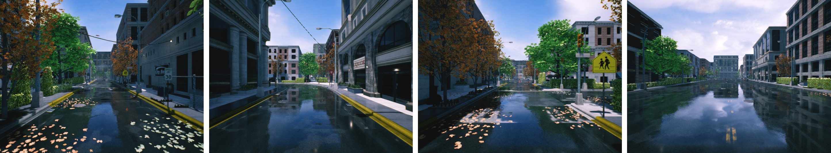
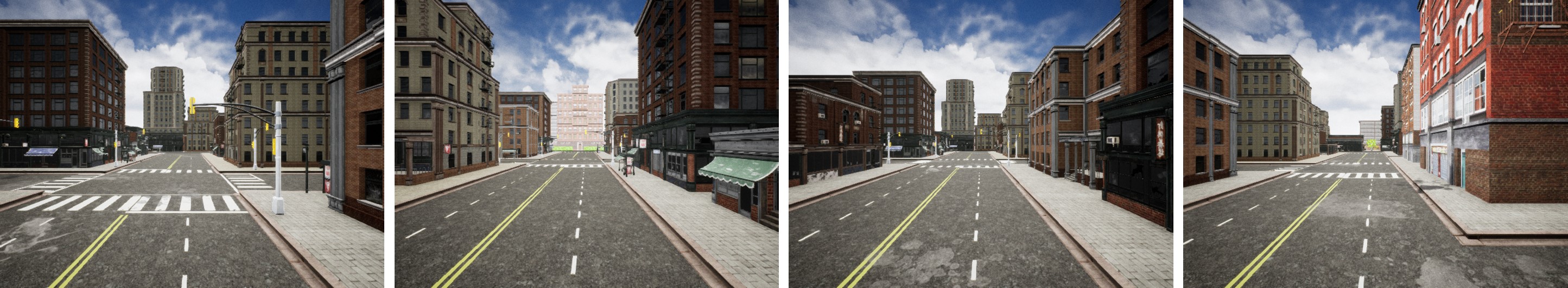
[5pt]  [5pt]  [5pt]

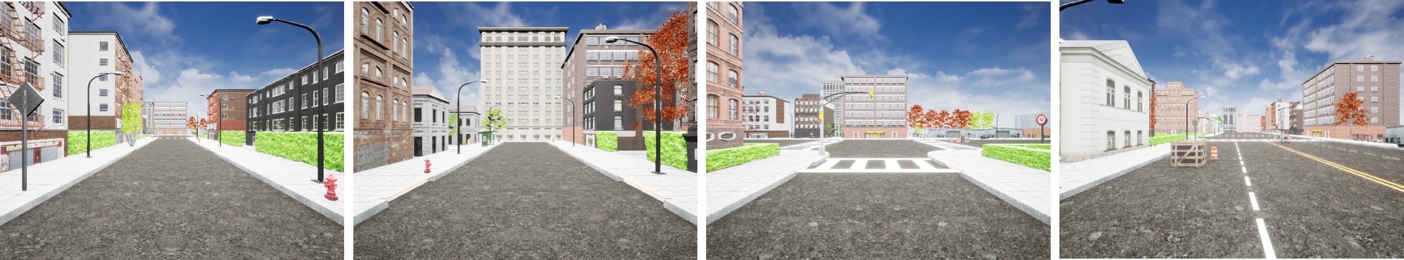
Figure 2: Examples of the synthetic dataset. The dataset consists of three different city environments, 24 scenes, and 3,333 frames.

Synthetic Dataset

In the field of computer vision, many deep learning-based methods have been proposed. However, deep learning networks for solving various computer vision problems require a large amount of dataset to train the network. Many methods require a large amount of image data and a label of each image to train the network, thus consuming substantial time and effort. To solve this problem, various methods that easily acquire data through synthetic environments have been proposed. Richter et al. [21] proposed a method that easily acquires 3D scenes and labels by intervening in the communication process between the video game Grand Theft Auto V and the GPU. Ros et al. [22] proposed a method for acquiring 3D scene data by constructing a stereo camera on a virtual car after constructing a virtual city. Zhang et al. [40] used OpenGL for acquiring synthetic data. However, these methods only acquire a single or stereo synthetic image, and the limitation is that a user’s arbitrary scene is difficult to create. Qiu et al. [19] proposed the UnrealCV, a module for acquiring user arbitrary scenes based on Unreal Engine 4, an open-source game engine that can easily construct user arbitrary scenes. In this paper, we use UnrealCV to construct a virtual city and a light field camera and then acquire synthetic light field data as shown in Figure 2.

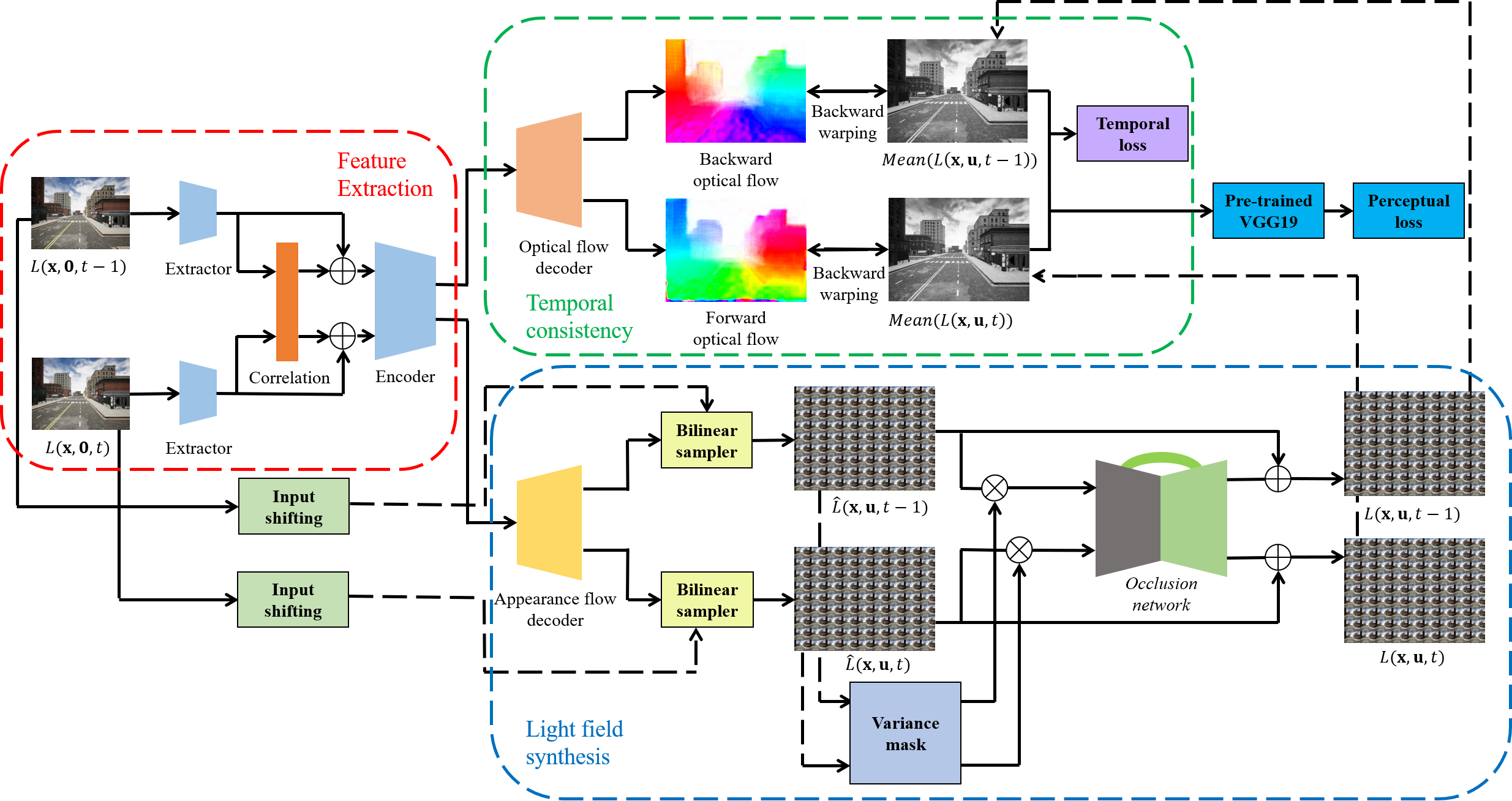
Figure 3: Proposed deep learning framework. The overall framework is divided into 3 parts, i.e. a feature extraction for extracting the features from each frame of the input video, 5D light field video synthesis, and temporal consistency refinement. After extracting the features by considering the correlation between adjacent frames, the light field video is synthesized by estimating both optical flow and appearance flow, and by refining using variance mask.

3 Proposed Method

In this paper, we propose a method for synthesizing 5D light field video ${L}(\textbf{x},\textbf{u},t)$ from a monocular video ${L}(\textbf{x},\textbf{0},t)$. We parameterize the light field video as ${L}(\textbf{x},\textbf{u},t)$ following [13]. x and u denote the coordinate vector in the spatial domain $(x,y)$ and the angular domain $(u,v)$ of the light field, respectively. We represent the light field video synthesis as an approximation function $f(\cdot)$ as follows:

$${L}(\textbf{x},\textbf{u},t)=f({L}(\textbf{x},\textbf{0},t)).$$ (1)

Figure 3 shows the proposed deep learning framework that synthesizes 5D light field video from the input monocular video. The overall framework is divided into three sections, namely, a feature extraction for extracting the features from each frame of the input video, 5D light field video synthesis, and temporal consistency refinement. Since the ground truth appearance flow and optical flow are computationally expensive and difficult, the proposed framework estimates the appearance flow and optical flow by training through an unsupervised approach.

3.1 Feature Extraction

${L}(\textbf{x},\textbf{0},t-1)$, and ${L}(\textbf{x},\textbf{0},t)$ are initially converted into the luminance images for memory efficiency to extract the feature from the input monocular video frame. The initial feature $\xi_{t}^{(l)}$ is extracted using an initial feature extraction encoder $\phi_{init}$, which consists of four convolution layers. The process of extracting the initial feature can be described as follows:

$$\xi_{t}^{(l)}=\phi_{init}^{(l)}({L}(\textbf{x},\textbf{0},t))$$ (2)

where $\phi_{init}^{(l)}(\cdot)$ represents feature activation in the $l_{\rm th}$ layer of the initial feature extraction encoder $\phi_{init}$. The extracted initial features are passed through the correlation layer in consideration of the correlation between two adjacent video frames, namely, ${L}(\textbf{x},\textbf{0},t-1)$ and ${L}(\textbf{x},\textbf{0},t)$. The encoder $\phi_{fin}$ extracts the final feature $\zeta_{t}$ and $\zeta_{t-1}$ by combining the obtained correlation information and the initial features. The process of extracting the final feature can be described as follows:

$$\zeta_{t}=\phi_{fin}(corr(\xi_{t}^{(4)},\xi_{t-1}^{(4)}),conv(\xi_{t}^{(4)}))$$ (3)

$$\zeta_{t-1}=\phi_{fin}(corr(\xi_{t-1}^{(4)},\xi_{t}^{(4)}),conv(\xi_{t-1}^{(4)}))$$ (4)

where $corr$ and $conv$ represent the correlation and convolution layers, respectively.

3.2 Light Field Synthesis

Appearance Flow Estimation

The appearance flow decoder $\varphi_{f}$, which takes the encoded feature map $\zeta_{t}$ obtained from Eq. (3), estimates the appearance flow ${L}_{f}(\textbf{x},\textbf{u},t)$ corresponding to each SAI at time $t$. Using estimated appearance flow, we synthesize the initial light field video frame $\hat{L}(\textbf{x},\textbf{u},t)$ by warping shifted input images ${L}_{s}(\textbf{x},\textbf{u},t)$ and estimated appearance flow for each angular coordinate. The initial light field synthesis can be written as follows:

$$\hat{L}(\textbf{x},\textbf{u},t) =B({L}_{s}(\textbf{x},\textbf{u},t),{L}_{f}(\textbf{x},\textbf{u},t))$$ (5)

$${L}_{f}(\textbf{x},\textbf{u},t) =\varphi_{f}(\zeta_{t})$$ (6)

$${L}_{s}(\textbf{x},\textbf{u},t) =S({L}(\textbf{x},\textbf{0},t),\nabla(\textbf{u}))$$

$$={L}(x-(\eta\times\Delta{u}),y-(\eta\times\Delta{v}))$$ (7)

where $B$ is the warping function for synthesizing the light field using shifted input image ${L}_{s}(\textbf{x},\textbf{u},t)$ and its corresponding appearance flow ${L}_{f}(\textbf{x},\textbf{u},t)$. The warping function uses the bilinear sampler module [10] for generating initial light field video frame $\hat{L}(\textbf{x},\textbf{u},t)$. $S$ is the input shifting technique, which shifts the central view to the position $\nabla(\textbf{u})$ of the novel view. The input shifting technique eases the difficulty of training the network by working as the bias initialization. $\eta$ is a shift constant based on the disparity between each SAI. We use the light field mean and variance losses $\ell_{local}$, $\ell_{global}$ proposed by [9] for training the appearance flow decoder.

Occlusion Network

The synthesized light field video frame obtained by Eq. (5) has a limitation, i.e., the synthesis result of the image boundary and occluded region is poor due to the nature of appearance flow. As shown in Figure 4, a 9$\times$9 variance mask $Mask(\hat{L})$ is formed using $\hat{L}(\textbf{x},\textbf{u},t)$’s variance image $Var(\hat{L})$ to overcome this limitation. The variance image of the light field represents a difference between each SAI, which is the occluded region of the scene. To improve the quality of the occluded, edged, and boundary regions of the synthesized light field video frame, we propose Occlusion Network, which improves the quality of the synthesized light field video frame by inputting the synthesized light field video frame and the variance mask. Figure 4 visualizes the variance image and mask. Different from the 2D image, the light field image has an angular dimension in addition to the spatial dimension. To handle both dimensions simultaneously, Occlusion Network is constructed using the 3D convolution layers instead of the 2D convolution layers. Occlusion Network has a 3D encoder-decoder structure with $\hat{L}(\textbf{x},\textbf{u},t)$ and $Var(\hat{L})$ as inputs. To preserve the information of the angular dimension, Occlusion Network maintains the size of the angular dimension while reducing the spatial resolution when it passes through the encoder layers. By contrast, the decoder layer increases the spatial resolution while maintaining the size of the angular dimension. The final light field video frame ${L}(\textbf{x},\textbf{u},t)$ is obtained by adding $\hat{L}(\textbf{x},\textbf{u},t)$ and the residual image $R(\textbf{x},\textbf{u},t)$ obtained at the last stage of the decoder layer, which can be described as follows:

$${L}(\textbf{x},\textbf{u},t)=O(\hat{L}(\textbf{x},\textbf{u},t),Var(\hat{L}))+\hat{L}(\textbf{x},\textbf{u},t)$$ (8)

where $O(\cdot)$ represents the Occlusion Network. We train the Occlusion Network by minimizing the simple L1 error as follows:

$$\ell_{occ}=||{L}(\textbf{x},\textbf{u},t)-{L_{GT}}(\textbf{x},\textbf{u},t)||_{1}.$$ (9)

The 3D convolution is performed with the filter size 3$\times$3$\times$3, and leaky Relu [38] activation function. The last layer uses tanh activation function to force the pixel values of the residual image to [-1, 1].

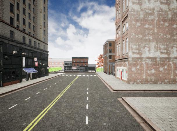
(a)

(b)

(c)

Figure 4: Light field variance mask. (a) Centerview. (b) Variance image of light field. (c) Variance mask.

Perceptual Loss

To improve the synthesized light field video frame’s quality, we use perceptual loss using the pre-trained VGG-19 network [25]. Perceptual loss has been used as a loss function in various deep learning-based methods; it has a similar tendency to human perception [39]. Computing perceptual loss for all SAIs of light field video frames is computationally heavy. Therefore, we calculate and optimize the perceptual loss for the mean image of the synthesized light field video frame. Perceptual loss can be described as follows:

$$\ell_{percep}=|| \phi_{VGG}^{(3)}(Mean(L(\textbf{x},\textbf{u},t)))-$$ (10)

$$\phi_{VGG}^{(3)}(Mean(L_{GT}(\textbf{x},\textbf{u},t)))||_{1}$$

where $\phi_{VGG}^{(n)}(\cdot)$ represents the $n_{\rm th}$ feature activation of the VGG-19 network. We use the third layer’s feature activation which contains low-level features to calculate the perceptual loss.

3.3 Temporal Consistency

In general, an optical flow between each frame is estimated and warped to a target frame to minimize the difference between the warped frame and target frame and provide temporal consistency to a video. However, estimating the optical flow for every 9$\times$9 SAIs in the light field video frame is difficult. Therefore, we do not estimate the optical flow for all 9$\times$9 SAIs, but we estimate the optical flow for the mean image of the light field video frame $Mean(\hat{L})$ and use it to maintain temporal consistency. To estimate the optical flow, we use the features extracted from $\phi_{init}$ and $\phi_{fin}$ and the loss function in [16]. To obtain the accurate optical flow for the light field image, we estimate the optical flow between the input video frames ${L}(\textbf{x},\textbf{0},t)$ and ${L}(\textbf{x},\textbf{0},t-1)$. After the network that synthesizes the initial light field image is trained to some level, the two synthesized initial light field video frames $\hat{L}(\textbf{x},\textbf{u},t)$ and $\hat{L}(\textbf{x},\textbf{u},t-1)$ are used instead of the two input video frames. Using the mean image of the light fields $\hat{L}(\textbf{x},\textbf{u},t)$ and $\hat{L}(\textbf{x},\textbf{u},t-1)$, we estimate and warp the optical flow to ${(t-1)\rightarrow t}$ and ${t\rightarrow(t-1)}$. The temporal consistency is obtained by minimizing the difference between the mean image of the warped image and the target light field image as follows:

$$\ell_{temp}=|| M(\omega(Mean({L}(\textbf{x},\textbf{u},t)),{O}_{t\rightarrow t-1}))-$$ (11)

$$M(Mean({L}(\textbf{x},\textbf{u},t-1)))||_{1}+$$

$$|| M(\omega(Mean({L}(\textbf{x},\textbf{u},t-1)),{O}_{t-1\rightarrow t}))-$$

$$M(Mean({L}(\textbf{x},\textbf{u},t)))||_{1}$$

where $M$ is the valid mask generated using forward and backward optical flow as proposed by [44]. The valid mask uses the assumption that the vectors must be in the same position when the vectors of the estimated optical flow is forwarded and then moved backward. If the pixel’s location satisfies the hypothesis, the pixel value is set to 1, and the other value is set to 0 to form a valid mask.

4 Experimental Results

We evaluate the proposed method qualitatively and quantitatively. The performance is compared with the state-of-the-art methods for single image light field synthesis [27] and [9] because no prior work was conducted on light field video synthesis. Moreover, no ground truth light field video dataset is avaliable. Thus, we use the synthetic light field video dataset for the quantitative evaluation. Test data consist of 162 frames that are unused in the training. The qualitative evaluation is performed on the KITTI [6] dataset, which is an actual scene dataset. The spatial resolution of the training light field video data used in this paper is 480$\times$640, and the resolution of the original KITTI data is 375$\times$1242. Therefore, the light field is synthesized by changing the input resolution to 480$\times$640 using the bicubic interpolation. The proposed framework is implemented with TensorFlow [2]. While training, we randomly crop the input light field spatial resolution into 224$\times$224.

We train our network end-to-end on NVIDIA Titan RTX D6 24GB GPU, 16GB RAM, and Intel Core i9-9900X CPU @3.50GHz CPU using the Adam optimizer with default parameter $\beta_{1}=0.9$, $\beta_{2}=0.999$ and learning rate $\alpha=0.0002$. The optical flow decoder and appearance flow decoder run for the first 50K iterations, and then every sub-networks run together. More technical details are described in the supplementary material.

Temporal Stability

To evaluate the temporal stability of the synthesized light field video, we calculate the temporal stability with optical flow-based warping error based on [12] as follows:

$$E_{temp}(L(\textbf{x},\textbf{u},t),L(\textbf{x},\textbf{u},t-1))$$ (12)

$$=\frac{1}{UV-1}\displaystyle\sum_{\textbf{u}=\textbf{-4}}^{\textbf{4}}\left[\frac{||\tilde{L}(\textbf{x},\textbf{u},t)-L(\textbf{x},\textbf{u},t-1)||_{1}}{\displaystyle\sum_{n=1}^{N}M^{(n)}}\right],\textbf{u}\neq\textbf{0}$$

where $U$, and $V$ denote the size of each angular dimension and $M^{(n)}$ denotes the $nth$ pixel that has a value of 1 in the valid mask among $N$ pixels. $\tilde{L}(\textbf{x},\textbf{u},t)$ denotes the frame warped $L(\textbf{x},\textbf{u},t)$ at time $t-1$.

4.1 Qualitative Evaluation

We perform the qualitative evaluation of the proposed method on the KITTI dataset. For comparison, after synthesizing the light field video from the input video, we estimate the depth using the synthesized light field video frames to evaluate the quality of synthesized light field video frame. We use CAE [34], which is the traditional light field depth estimation method. Figure 5 shows the qualitative evaluation on the KITTI dataset. As shown in Figure 5, the results from [27] show the insufficient degree of EPI slope and fail to estimate the accurate depth from the synthesized light field frame for some regions of the scene. [9] failed to synthesize the light field given that it failed to estimate the accurate appearance flow for some regions of the scene. In addition, [27] and [9] synthesized temporally inconsistent light field video given that the estimated depth of the light field frames are not temporally consistent. Note that, although it is trained with synthetic dataset, the proposed method synthesizes temporally consistent light field compared with other methods. Moreover, we show the refocusing effect of the synthesized light field video in Figure 6.

Dataset		Synthetic #1			Synthetic #2
Metric		PSNR	SSIM		PSNR	SSIM
[27]		22.56	0.696		24.99	0.735
[9]		23.52	0.708		26.76	0.804
Proposed		23.77	0.732		27.11	0.831

Table 1: Average PSNR (in dB) and SSIM for two synthetic test sets. Each test set consists of 162 frames.

4.2 Quantitative Evaluation

To evaluate the proposed method quantitatively, we use PSNR and SSIM [30]. The average PSNR and SSIM for each test set are listed in Table 1. We use synthetic test sets #1 and #2 to perform a quantitative comparison between the proposed method and the existing state-of-the-art methods. The test set #1 has a similar appearance to the first row of Figure 2, and test set #2 is similar to the second and third rows of Figure 2. The test set #1 is more challenging because it consists of specular reflection and high frequency components. As shown in Table 1, for the synthetic test set #1, the proposed method outperforms the existing state-of-the-art methods by 1.2 and 0.2 dB in terms of PSNR and 0.03 and 0.02 in terms of SSIM. For the synthetic test set #2, the proposed method outperforms the previous methods by 2 and 0.3 dB in PSNR and 0.09 and 0.02 in SSIM.

Input

(a)

(b)

(c)

(d)

(e)

(f)

(g)

(h)

(i)

[27]

(j)

(k)

(l)

(m)

(n)

(o)

(p)

(q)

(r)

[9]

(s)

(t)

(u)

(v)

(w)

(x)

(y)

(z)

(aa)

Proposed

(ab)

(ac)

(ad)

(ae)

(af)

(ag)

(ah)

(ai)

(aj)

Input

(ak)

(al)

(am)

(an)

(ao)

(ap)

(aq)

(ar)

(as)

[27]

(at)

(au)

(av)

(aw)

(ax)

(ay)

(az)

(ba)

(bb)

[9]

(bc)

(bd)

(be)

(bf)

(bg)

(bh)

(bi)

(bj)

(bk)

Proposed

(bl)

(bm)

(bn)

(bo)

(bp)

(bq)

(br)

(bs)

(bt)

Input

(bu)

(bv)

(bw)

(bx)

(by)

(bz)

(ca)

(cb)

(cc)

[27]

(cd)

(ce)

(cf)

(cg)

(ch)

(ci)

(cj)

(ck)

(cl)

[9]

(cm)

(cn)

(co)

(cp)

(cq)

(cr)

(cs)

(ct)

(cu)

Proposed

(cv)

(cw)

(cx)

(cy)

(cz)

(da)

(db)

(dc)

(dd)

Figure 5: Qualitative comparison on the KITTI dataset. We show the eight continuous input video frames, their estimated depth after being synthesized as a light field frame using each method, and EPIs.

Temporal Stability Evaluation

We use Eq. (12) to show that the synthesized light field video is temporally consistent. Eq. (12) warps an image at time ($t$) for each SAI to time ($t-1$) and calculates a warping error within a valid mask. We perform this computation on all SAIs except for the center view because it is the same as the input frame. Table 2 shows the numerical values obtained by performing this process for the entire video and then averaging the warping error over the entire video. As shown in Table 2, the proposed method can synthesize a light field video that is more stable in the temporal domain in comparison with existing methods.

Dataset		Synthetic #1		Synthetic #2
[27]		140.38		643.02
[9]		139.45		642.70
Proposed		138.72		635.57

Table 2: Temporal stability evaluation for each test set.

Figure 6: Video refocusing application. We show the four continuous frames focused on the white car on the left of the scene.

4.3 Ablation study

To determine the effect of each loss function, we evaluate the proposed network by excluding each loss function $\ell_{temp}$, $\ell_{percep}$, and $\ell_{occ}$ and train the proposed network. The ablation study for the loss functions $\ell_{global}$ and $\ell_{local}$ which are proposed by [9] is not performed. Table 3 shows the quantitative evaluation when excluding each loss function one by one.

Dataset		Synthetic #1			Synthetic #2
Metric		PSNR	SSIM		PSNR	SSIM
without $\ell_{temp}$		23.58	0.688		22.82	0.646
without $\ell_{percep}$		21.47	0.644		24.21	0.697
without $\ell_{occ}$		21.62	0.632		21.77	0.602
without $corr$		23.45	0.717		24.52	0.723
Proposed		23.77	0.732		27.11	0.831

Table 3: Quantitative evaluation of excluding each loss function’s effect on the networks.

Temporal Loss

For the test set #1, which has many non-Lambertian elements, when the temporal loss function $\ell_{temp}$ is excluded, the degradation is approximately 0.2 dB in PSNR and 0.04 in SSIM, respectively. By contrast, for the dataset #2 with a relatively simpler structure compared with dataset #1, the difference in PSNR and SSIM is approximately 4 dB and 0.19, respectively. This result indicates that the temporal consistency loss provides a considerable boost to the network performance for the simple scenes.

Perceptual Loss

Contrary to $\ell_{temp}$, for the dataset with multiple non-Lambertian elements, the effect of excluding perceptual loss is approximately 2 dB in PSNR and 0.9 in SSIM, respectively. For dataset # 2, the effect of perceptual loss is relatively smaller than that of temporal loss; the effect is approximately 3 dB in PSNR and 0.13 in SSIM. The perceptual loss works effectively on a scene that has many non-Lambertian elements rather than temporal loss.

Occlusion Loss

In the case of $\ell_{occ}$, which indicates the influence of Occlusion Network on the network, the effect is the greatest for datasets # 1 and #2, except for the PSNR value of the dataset #1. Excluding the network, the result shows that PSNR and SSIM values decrease to approximately 2 dB and 0.1 for dataset #1 and approximately 5 dB and 0.2 for dataset #2.

Correlation Layer

We also train our network without correlation layer. The effect of excluding the correlation layer is the least among the others. The PSNR and SSIM values decrease to approximately 0.2 dB and 0.01 for the dataset #1 and approximately 2.5 dB and 0.11 for dataset #2. It indicates that the correlation information from both frames works similar to temporal consistency loss. Even though the effect is the least, excluding only a single correlation layer affects the performance significantly for simple scenes, such as test set #2.

5 Conclusion

In this paper, we proposed a method for synthesizing 5D light field video with 9$\times$9 SAIs that is temporally consistent from a monocular video using synthetic light field datasets. The proposed method considered the correlation between adjacent frames of the input monocular video and estimated the appearance flow, forward and backward optical flow using the extracted features. The initial light field video was synthesized using the estimated appearance flow and provided temporal consistency to synthesized video using the estimated optical flow obtained using the mean image of the synthesized light field image. In addition, a binary mask was formed using a variance image of the initial light field video frame. It was used to improve the quality of occlusion and edge regions of the initial light field video frame using the proposed Occlusion NetworkṪhe experimental results showed that the method was superior to the existing state-of-the-art methods quantitatively and qualitatively. We analyzed the effects of each loss function through an ablation study and proposed an effective loss function were many non-Lambertian elements exist in the scene and when non. The experimental results showed that the network trained using synthetic light field datasets can be generalized effectively for the datasets comprising actual scenes in addition to 3D graphic scenes. We hope that our dataset and experimental results motivate researchers to solve the light field video synthesis problem.

References

- [1] Raytrix 3D light field camera. https://raytrix.de/products/. Accessed: 2019-11-08.
- [2] Martín Abadi, Paul Barham, Jianmin Chen, Zhifeng Chen, Andy Davis, Jeffrey Dean, Matthieu Devin, Sanjay Ghemawat, Geoffrey Irving, Michael Isard, et al. Tensorflow: A system for large-scale machine learning. In 12th Symposium on Operating Systems Design and Implementation (16), pages 265–283, 2016.
- [3] Nicolas Bonneel, James Tompkin, Kalyan Sunkavalli, Deqing Sun, Sylvain Paris, and Hanspeter Pfister. Blind video temporal consistency. ACM Trans. on Graphics, 34(6):196, 2015.
- [4] John Flynn, Ivan Neulander, James Philbin, and Noah Snavely. Deepstereo: Learning to predict new views from the world’s imagery. In Proc. of IEEE Conference on Computer Vision and Pattern Recognition, pages 5515–5524, 2016.
- [5] Ravi Garg, Vijay Kumar BG, Gustavo Carneiro, and Ian Reid. Unsupervised cnn for single view depth estimation: Geometry to the rescue. In Proc. of European Conference on Computer Vision, pages 740–756, 2016.
- [6] Andreas Geiger, Philip Lenz, and Raquel Urtasun. Are we ready for autonomous driving? the kitti vision benchmark suite. In Proc. of IEEE Conference on Computer Vision and Pattern Recognition, pages 3354–3361, 2012.
- [7] Clément Godard, Oisin Mac Aodha, and Gabriel J Brostow. Unsupervised monocular depth estimation with left-right consistency. In Proc. of IEEE Conference on Computer Vision and Pattern Recognition, pages 270–279, 2017.
- [8] Po-Han Huang, Kevin Matzen, Johannes Kopf, Narendra Ahuja, and Jia-Bin Huang. Deepmvs: Learning multi-view stereopsis. In Proc. of IEEE Conference on Computer Vision and Pattern Recognition, pages 2821–2830, 2018.
- [9] Andre Ivan and In Kyu Park. Synthesizing a 4d spatio-angular consistent light field from a single image. arXiv preprint arXiv:1903.12364, 2019.
- [10] Max Jaderberg, Karen Simonyan, and Andrew Zisserman. Spatial transformer networks. In Advances in Neural Information Processing Systems, pages 2017–2025, 2015.
- [11] Nima Khademi Kalantari, Ting-Chun Wang, and Ravi Ramamoorthi. Learning-based view synthesis for light field cameras. ACM Trans. on Graphics, 35(6):193, 2016.
- [12] Wei-Sheng Lai, Jia-Bin Huang, Oliver Wang, Eli Shechtman, Ersin Yumer, and Ming-Hsuan Yang. Learning blind video temporal consistency. In Proc. of European Conference on Computer Vision, pages 170–185, 2018.
- [13] Marc Levoy and Pat Hanrahan. Light field rendering. In Proc. of SIGGRAPH, pages 31–42, 1996.
- [14] Nianyi Li, Jinwei Ye, Yu Ji, Haibin Ling, and Jingyi Yu. Saliency detection on light field. In Proc. of IEEE Conference on Computer Vision and Pattern Recognition, pages 2806–2813, 2014.
- [15] Gabriel Lippmann. Epreuves reversibles donnant la sensation du relief. Journal of Theoretical and Applied Physics, 7(1):821–825, 1908.
- [16] Simon Meister, Junhwa Hur, and Stefan Roth. Unflow: Unsupervised learning of optical flow with a bidirectional census loss. In Proc. of AAAI Conference on Artificial Intelligence, pages 7251–7259, 2018.
- [17] Ben Mildenhall, Pratul P. Srinivasan, Rodrigo Ortiz-Cayon, Nima Khademi Kalantari, Ravi Ramamoorthi, Ren Ng, and Abhishek Kar. Local light field fusion: Practical view synthesis with prescriptive sampling guidelines. ACM Trans. on Graphics, 2019.
- [18] Ren Ng, Marc Levoy, Mathieu Brédif, Gene Duval, Mark Horowitz, Pat Hanrahan, et al. Light field photography with a hand-held plenoptic camera. Computer Science Technical Report CSTR, 2(11):1–11, 2005.
- [19] Weichao Qiu and Alan Yuille. Unrealcv: Connecting computer vision to unreal engine. In Proc. of European Conference on Computer Vision, pages 909–916, 2016.
- [20] Stephan R Richter, Zeeshan Hayder, and Vladlen Koltun. Playing for benchmarks. In Proc. of IEEE International Conference on Computer Vision, pages 2213–2222, 2017.
- [21] Stephan R Richter, Vibhav Vineet, Stefan Roth, and Vladlen Koltun. Playing for data: Ground truth from computer games. In Proc. of European Conference on Computer Vision, pages 102–118, 2016.
- [22] German Ros, Laura Sellart, Joanna Materzynska, David Vazquez, and Antonio M Lopez. The synthia dataset: A large collection of synthetic images for semantic segmentation of urban scenes. In Proc. of IEEE Conference on Computer Vision and Pattern Recognition, pages 3234–3243, 2016.
- [23] Hendrik Schilling, Maximilian Diebold, Carsten Rother, and Bernd Jähne. Trust your model: Light field depth estimation with inline occlusion handling. In Proc. of IEEE Conference on Computer Vision and Pattern Recognition, pages 4530–4538, 2018.
- [24] Changha Shin, Hae-Gon Jeon, Youngjin Yoon, In So Kweon, and Seon Joo Kim. Epinet: A fully-convolutional neural network using epipolar geometry for depth from light field images. In Proc. of IEEE Conference on Computer Vision and Pattern Recognition, pages 4748–4757, 2018.
- [25] Karen Simonyan and Andrew Zisserman. Very deep convolutional networks for large-scale image recognition. arXiv preprint arXiv:1409.1556, 2014.
- [26] Pratul P Srinivasan, Richard Tucker, Jonathan T Barron, Ravi Ramamoorthi, Ren Ng, and Noah Snavely. Pushing the boundaries of view extrapolation with multiplane images. In Proc. of IEEE Conference on Computer Vision and Pattern Recognition, pages 175–184, 2019.
- [27] Pratul P Srinivasan, Tongzhou Wang, Ashwin Sreelal, Ravi Ramamoorthi, and Ren Ng. Learning to synthesize a 4d rgbd light field from a single image. In Proc. of IEEE International Conference on Computer Vision, pages 2243–2251, 2017.
- [28] Ting-Chun Wang, Jun-Yan Zhu, Nima Khademi Kalantari, Alexei A Efros, and Ravi Ramamoorthi. Light field video capture using a learning-based hybrid imaging system. ACM Trans. on Graphics, 36(4):133, 2017.
- [29] Yunlong Wang, Fei Liu, Zilei Wang, Guangqi Hou, Zhenan Sun, and Tieniu Tan. End-to-end view synthesis for light field imaging with pseudo 4dcnn. In Proc. of European Conference on Computer Vision, pages 333–348, 2018.
- [30] Zhou Wang, Alan C Bovik, Hamid R Sheikh, Eero P Simoncelli, et al. Image quality assessment: from error visibility to structural similarity. IEEE Trans. on Image Processing, 13(4):600–612, 2004.
- [31] Sven Wanner and Bastian Goldluecke. Variational light field analysis for disparity estimation and super-resolution. IEEE Trans. on Pattern Analysis and Machine Intelligence, 36(3):606–619, 2013.
- [32] Bennett Wilburn, Neel Joshi, Vaibhav Vaish, Eino-Ville Talvala, Emilio Antunez, Adam Barth, Andrew Adams, Mark Horowitz, and Marc Levoy. High performance imaging using large camera arrays. ACM Trans. on Graphics, 24(3):765–776, 2005.
- [33] Williem and In Kyu Park. Robust light field depth estimation for noisy scene with occlusion. In Proc. of IEEE Conference on Computer Vision and Pattern Recognition, pages 4396–4404, 2016.
- [34] Williem, In Kyu Park, and Kyoung Mu Lee. Robust light field depth estimation using occlusion-noise aware data costs. IEEE Trans. on Pattern Analysis and Machine Intelligence, 40(10):2484–2497, 2017.
- [35] Henry Wing Fung Yeung, Junhui Hou, Jie Chen, Yuk Ying Chung, and Xiaoming Chen. Fast light field reconstruction with deep coarse-to-fine modeling of spatial-angular clues. In Proc. of European Conference on Computer Vision, pages 137–152, 2018.
- [36] Gaochang Wu, Mandan Zhao, Liangyong Wang, Qionghai Dai, Tianyou Chai, and Yebin Liu. Light field reconstruction using deep convolutional network on epi. In Proc. of IEEE Conference on Computer Vision and Pattern Recognition, pages 6319–6327, 2017.
- [37] Junyuan Xie, Ross Girshick, and Ali Farhadi. Deep3d: Fully automatic 2d-to-3d video conversion with deep convolutional neural networks. In Proc. of European Conference on Computer Vision, pages 842–857, 2016.
- [38] Bing Xu, Naiyan Wang, Tianqi Chen, and Mu Li. Empirical evaluation of rectified activations in convolutional network. arXiv preprint arXiv:1505.00853, 2015.
- [39] Richard Zhang, Phillip Isola, Alexei A Efros, Eli Shechtman, and Oliver Wang. The unreasonable effectiveness of deep features as a perceptual metric. In Proc. of IEEE Conference on Computer Vision and Pattern Recognition, pages 586–595, 2018.
- [40] Yinda Zhang, Shuran Song, Ersin Yumer, Manolis Savva, Joon-Young Lee, Hailin Jin, and Thomas Funkhouser. Physically-based rendering for indoor scene understanding using convolutional neural networks. In Proc. of IEEE Conference on Computer Vision and Pattern Recognition, pages 5287–5295, 2017.
- [41] Zhoutong Zhang, Yebin Liu, and Qionghai Dai. Light field from micro-baseline image pair. In Proc. of IEEE Conference on Computer Vision and Pattern Recognition, pages 3800–3809, 2015.
- [42] Tinghui Zhou, Richard Tucker, John Flynn, Graham Fyffe, and Noah Snavely. Stereo magnification: learning view synthesis using multiplane images. ACM Trans. on Graphics, 37(4):65, 2018.
- [43] Tinghui Zhou, Shubham Tulsiani, Weilun Sun, Jitendra Malik, and Alexei A Efros. View synthesis by appearance flow. In Proc. of European Conference on Computer Vision, pages 286–301, 2016.
- [44] Yuliang Zou, Zelun Luo, and Jia-Bin Huang. Df-net: Unsupervised joint learning of depth and flow using cross-task consistency. In Proc. of European Conference on Computer Vision, pages 36–53, 2018.