Matching for a family of infinite measure continued fraction transformations

Abstract.

As a natural counterpart to Nakada’s $\alpha$-continued fraction maps, we study a one-parameter family of continued fraction transformations with an indifferent fixed point. We prove that matching holds for Lebesgue almost every parameter in this family and that the exceptional set has Hausdorff dimension 1. Due to this matching property, we can construct a planar version of the natural extension for a large part of the parameter space. We use this to obtain an explicit expression for the density of the unique infinite $\sigma$-finite absolutely continuous invariant measure and to compute the Krengel entropy, return sequence and wandering rate of the corresponding maps.

1. Introduction

Over the past decades the dynamical phenomenon of matching, or synchronisation, has surfaced increasingly often in the study of the dynamics of interval maps, mostly due to the fact that systems with matching exhibit properties that resemble those of Markov maps. A map $T$ is said to have the matching property if for any discontinuity point $c$ of the map $T$ or its derivative $T^{\prime}$ the orbits of the left and right limits of $c$ eventually meet. That is, there exist non-negative integers $M$ and $N$, called matching exponents, such that

(1) $$T^{M}(c^{-})=T^{N}(c^{+}),$$

where

$$c^{-}=\lim_{x\uparrow c}T(x)\quad\text{and }\quad c^{+}=\lim_{x\downarrow c}T(x).$$

General results on the implications of matching are scarce. There are many results however on the consequences of matching for specific families of interval maps. In [KS12, BSORG13, BCK17, BCMP18, CM18, DK17] matching was considered for various families of piecewise linear maps in relation to expressions for the invariant densities, entropy and multiple tilings. Another type of transformation for which matching has proven to be convenient is for continued fraction maps, most notably for Nakada’s $\alpha$-continued fraction maps. This family was introduced in [Nak81] by defining for each $\alpha\in\big{[}\frac{1}{2},1\big{]}$ the map $S_{\alpha}:[\alpha-1,\alpha]\to[\alpha-1,\alpha]$ by $S_{\alpha}(0)=0$ and for $x\neq 0$,

(2) $$S_{\alpha}(x)=\Big{|}\frac{1}{x}\Big{|}-\Big{\lfloor}\Big{|}\frac{1}{x}\Big{|}+1-\alpha\Big{\rfloor}.$$

In [Nak81] Nakada constructed a planar natural extension of $S_{\alpha}$ and proved the existence of a unique absolutely continuous invariant probability measure. In [LM08] the family was extended to include the parameters $\alpha\in\big{[}0,\frac{1}{2}\big{)}$. On this part of the parameter space the planar natural extension strongly depends on the matching property, and it is much more complicated. This also affects the behaviour of the metric entropy as a function of $\alpha$, which is described in detail in [LM08, NN08, CMPT10, KSS12, CT13, Tio14]. In [DKS09, KU10, CIT18] matching was successfully considered for other families of continued fraction transformations.

The matching behaviour of these different families has some striking similarities. The parameter space usually breaks down into maximal intervals on which the exponents $M$ and $N$ from (1) are constant, called matching intervals. These matching intervals usually cover most of the space, leaving a Lebesgue null set. The set where matching fails, called the exceptional set, is often of positive Haussdorff dimension, see [CT12, KSS12, BCIT13, BCK17, DK17] for example.

So far, matching has been considered only for dynamical systems with a finite absolutely continuous invariant measure. In this article, we introduce and study the matching behaviour and its consequences for a one-parameter family of continued fraction transformations on the interval that have a unique absolutely continuous, $\sigma$-finite invariant measure that is infinite. This family of flipped $\alpha$-continued fraction transformations we introduce arises naturally as a counterpart to Nakada’s $\alpha$-continued fraction maps. Due to matching we obtain a nice planar natural extension on a large part of the parameter space, which allows us to explicitly compute dynamical features of the maps, such as the invariant density, Krengel entropy and wandering rate.

The family of maps $\{T_{\alpha}\}_{\alpha\in(0,1)}$ we consider is defined as follows. For each $\alpha\in(0,1)$ let

(3) $$D_{\alpha}=\bigcup_{n\geq 1}\Big{[}\frac{1}{n+\alpha},\frac{1}{n}\Big{]}\subseteq[0,1],$$

and $I_{\alpha}:=[\min\{\alpha,1-\alpha\},1]$, and define the map $T_{\alpha}:I_{\alpha}\to I_{\alpha}$ by

$$T_{\alpha}(x)=\left\{\begin{array}[]{l l}G(x)=\displaystyle\frac{1}{x}-\left\lfloor\frac{1}{x}\right\rfloor,&\text{if }x\in D_{\alpha}^{\mathsf{c}},\\[14.22636pt] 1-G(x)=\displaystyle-\frac{1}{x}+\left(1+\left\lfloor\frac{1}{x}\right\rfloor\right),&\text{if }x\in D_{\alpha},\end{array}\right.$$

where $G(x)=\frac{1}{x}\pmod{1}$ is the Gauss map and $D_{\alpha}^{\mathsf{c}}$ denotes the complement of $D_{\alpha}$ in $[0,1]$. Note that for $\alpha=0$ one recovers the Gauss map $G$, and $\alpha=1$ gives $1-G$, which is a shifted version of the Rényi map or backwards continued fraction map. Since these transformations have already been studied extensively, we omit them from our analysis. Figures 1(c) and 1(f) show the graphs of the maps $T_{\alpha}$ for a parameter $\alpha<\frac{1}{2}$ and a parameter $\alpha>\frac{1}{2}$, respectively. We could define $T_{\alpha}$ on the whole interval $[0,1]$, but since the dynamics of $T_{\alpha}$ is attracted to the interval $I_{\alpha}$ we just take that as the domain. Since $I_{\alpha}$ is bounded away from 0, any map $T_{\alpha}$ has only a finite number of branches. Note also that each map $T_{\alpha}$ has an indifferent fixed point at $1$.

We call these transformations flipped $\alpha$-continued fraction maps, due to their relation to the family of maps described in [MMY97]. The authors defined for each $\alpha\in[0,1]$ the folded $\alpha$-continued fraction map $\hat{S}_{\alpha}:[0,\max\{\alpha,1-\alpha\}]\to[0,\max\{\alpha,1-\alpha\}]$ by $\hat{S}_{\alpha}(0)=0$ and for $x\neq 0$,

$$\hat{S}_{\alpha}(x)=\Big{|}\frac{1}{x}-\Big{\lfloor}\frac{1}{x}+1-\alpha\Big{\rfloor}\Big{|}=\left\{\begin{array}[]{l l}G(x)=\displaystyle\frac{1}{x}-\left\lfloor\frac{1}{x}\right\rfloor,&\text{if }x\in D_{\alpha},\\[14.22636pt] 1-G(x)=\displaystyle-\frac{1}{x}+\left(1+\left\lfloor\frac{1}{x}\right\rfloor\right),&\text{if }x\in D_{\alpha}^{\mathsf{c}}.\end{array}\right.$$

The dynamical properties of the folded $\alpha$-continued fraction maps are essentially equal to those of Nakada’s $\alpha$-continued fraction maps. The name represents the idea that these maps ‘fold’ the interval $[\alpha-1,\alpha]$ onto $[0,\max\{\alpha,1-\alpha\}]$. As shown in Figure 1 the families $\{T_{\alpha}\}$ and $\{\hat{S}_{\alpha}\}$ are obtained by flipping the Gauss map on complementary parts of the unit interval and, as such, both families are particular instances of what are called $D$-continued fraction maps in [DHKM12]. Furthermore, for $\alpha=\frac{1}{2}$ the transformation $T_{\alpha}$ seems to be closely related, but not isomorphic, to the object of study of [DK00].

(a) $G$

(b) $\hat{S}_{\alpha}$

(c) $T_{\alpha}$

(d) $R=1-G$

(e) $\hat{S}_{\alpha}$

(f) $T_{\alpha}$

Figure 1. The Gauss map $G$ and the flipped map $R=1-G$ in (a) and (d). The folded $\alpha$-continued fraction map $\hat{S}_{\alpha}$ and the flipped $\alpha$-continued fraction map $T_{\alpha}$ for $\alpha<\frac{1}{2}$ in (b) and (c) and for $\alpha>\frac{1}{2}$ in (e) and (f).

The first main result of this article is on the matching behaviour of the family $T_{\alpha}$.

Theorem 1.1.

The set of parameters $\alpha\in(0,1)$ for which the transformation $T_{\alpha}$ does not have matching is a Lebesgue null set of full Hausdorff dimension.

We also give an explicit description of the matching intervals by relating them to the matching intervals of Nakada’s $\alpha$-continued fraction transformations. The matching behaviour allows us to construct a planar version of the natural extension for $\alpha\in(0,\frac{1}{2}\sqrt{2})$ leading to the following result.

Theorem 1.2.

Let $0\leq\alpha\leq\frac{1}{2}\sqrt{2}$, let $\mathcal{B}_{\alpha}$ be the Borel $\sigma$-algebra on $I_{\alpha}$ and let $g:=\frac{\sqrt{5}-1}{2}$. The absolutely continuous measure $\mu_{\alpha}$ on $(I_{\alpha},\mathcal{B}_{\alpha})$ with density

$$f_{\alpha}(x)=\left\{\begin{array}[]{l l}\frac{1}{x}\mathbf{1}_{[\alpha,\frac{\alpha}{1-\alpha}]}(x)+\frac{1}{1+x}\mathbf{1}_{[\frac{\alpha}{1-\alpha},1-\alpha]}(x)+\frac{2}{1-x^{2}}\mathbf{1}_{[1-\alpha,1]}(x),&\text{for }\alpha\in[0,\frac{1}{2}),\\ \frac{1}{1-x}\mathbf{1}_{[1-\alpha,\alpha]}(x)+\frac{1}{x(1-x)}\mathbf{1}_{[\alpha,\frac{1-\alpha}{\alpha}]}(x)+\frac{x^{2}+1}{x(1-x^{2})}\mathbf{1}_{[\frac{1-\alpha}{\alpha},1]}(x),&\text{for }\alpha\in[\frac{1}{2},g),\\ (\frac{1}{1-x}+\frac{1}{x+\frac{1}{g-1}})\mathbf{1}_{[1-\alpha,\frac{2\alpha-1}{\alpha}]}(x)+\frac{1}{1-x}\mathbf{1}_{[\frac{2\alpha-1}{\alpha},\alpha]}(x)+&\\ +(\frac{1}{1-x}+\frac{1}{x}-\frac{1}{x+\frac{1}{g}})\mathbf{1}_{[\alpha,\frac{2\alpha-1}{1-\alpha}]}(x)+\frac{x^{2}+1}{x(1-x^{2})}\mathbf{1}_{[\frac{2\alpha-1}{1-\alpha},1]}(x),&\text{for }\alpha\in[g,\frac{2}{3}),\\ (\frac{1}{1-x}+\frac{1}{x+\frac{1}{g-1}})\mathbf{1}_{[1-\alpha,\frac{2\alpha-1}{\alpha}]}(x)+\frac{1}{1-x}\mathbf{1}_{[\frac{2\alpha-1}{\alpha},\alpha]}(x)+&\\ +(\frac{1}{1-x}+\frac{1}{x}-\frac{1}{x+\frac{1}{g}})\mathbf{1}_{[\alpha,\frac{1-\alpha}{2\alpha-1}]}(x)+&\\ +(\frac{1}{1-x}+\frac{1}{x+1}-\frac{1}{x+\frac{1}{g}}+\frac{1}{x}-\frac{1}{x+\frac{1}{g+1}})\mathbf{1}_{[\frac{1-\alpha}{2\alpha-1},1]}(x),&\text{for }\alpha\in[\frac{2}{3},\frac{1}{2}\sqrt{2}),\\ \end{array}\right.$$

is the unique (up to scalar multiplication) $\sigma$-finite, infinite absolutely continuous invariant measure for $T_{\alpha}$. Furthermore, for $\alpha\in(0,g]$ the Krengel entropy equals $\frac{\pi^{2}}{6}$. For $\alpha\in(0,\frac{1}{2}\sqrt{2})$ the wandering rate is given by $w_{n}(T_{\alpha})\sim\log n$ and the return sequence by $a_{n}(T_{\alpha})\sim\frac{n}{\log n}$.

The paper is organised as follows. In the next section we give some preliminaries on continued fractions and explain how the maps $T_{\alpha}$ can be used to generate them for numbers in the interval $I_{\alpha}$. We also prove that the maps $T_{\alpha}$ fall into the family of what are called AFN-maps in [Zwe00]. In the third section we study the phenomenon of matching, leading to Theorem 1.1, and we give an explicit description of the matching intervals. The fourth section is devoted to defining a planar natural extension for the maps $T_{\alpha}$ for $\alpha<\frac{1}{2}\sqrt{2}$. This is then used to obtain the invariant densities appearing in Theorem 1.2. In the last section we compute the Krengel entropy, wandering rate and return sequence for $T_{\alpha}$, giving the last part of Theorem 1.2.

2. Preliminaries

2.1. Semi-regular continued fraction expansions

In 1913, Perron introduced the notion of semi-regular continued fraction expansions, which are finite or infinite expressions for real numbers of the following form:

$$x=d_{0}+\cfrac{\epsilon_{0}}{d_{1}+\cfrac{\epsilon_{1}}{d_{2}+\ddots+\cfrac{\epsilon_{n-1}}{d_{n}+\ddots}}},$$

where $d_{0}\in\mathbb{Z}$ and for each $n\geq 1$, $\epsilon_{n-1}\in\{-1,1\}$, $d_{n}\in\mathbb{N}$ and $d_{n}+\epsilon_{n}\geq 1$; see for example [Per57]. We denote the semi-regular continued fraction expansion of a number $x$ by

$$x=[d_{0};\epsilon_{0}/d_{1},\epsilon_{1}/d_{2},\epsilon_{2}/d_{3},\ldots].$$

The maps $T_{\alpha}$ generate semi-regular continued fraction expansions of real numbers by iteration. Define for any $\alpha\in(0,1)$ and any $x\in I_{\alpha}$ the partial quotients $d_{k}=d_{k}(x)=d_{1}(T^{k-1}_{\alpha}(x))$ and the signs $\epsilon_{k}=\epsilon_{k}(x)=\epsilon_{1}(T^{k-1}_{\alpha}(x))$ by setting

$$d_{1}(x):=\begin{cases}\lfloor\frac{1}{x}\rfloor,&\text{if }x\in D_{\alpha}^{\mathsf{c}},\\ \lfloor\frac{1}{x}\rfloor+1,&\text{otherwise};\end{cases}\quad\text{ and }\quad\epsilon_{1}(x):=\begin{cases}1,&\text{if }x\in D_{\alpha}^{\mathsf{c}},\\ -1,&\text{otherwise}.\end{cases}$$

With this notation the map $T_{\alpha}$ can be written as $T_{\alpha}(x)=\epsilon_{1}(x)\big{(}\frac{1}{x}-d_{1}(x)\big{)}$, implying

(4) $$x=\frac{1}{d_{1}+\epsilon_{1}T_{\alpha}(x)}=\cfrac{1}{d_{1}+\cfrac{\epsilon_{1}}{d_{2}+\ddots+\cfrac{\epsilon_{n-1}}{d_{n}+\epsilon_{n}T^{n}_{\alpha}(x)}}}.$$

Denote by $(p_{n}/q_{n})_{n\geq 1}$ the sequence of convergents of such an expansion, that is,

$$p_{n}/q_{n}=[0;1/d_{1},\epsilon_{1}/d_{2},\ldots,\epsilon_{n-1}/d_{n}].$$

Since we obtained $T_{\alpha}$ from the Gauss map, by flipping on the domain $D_{\alpha}$ from (3), it follows from [DHKM12, Theorem 1] that for any $x\in I_{\alpha}$ we have: $\displaystyle\lim_{n\rightarrow\infty}\frac{p_{n}}{q_{n}}=x$. Therefore, we can write

$$x=\cfrac{1}{d_{1}+\cfrac{\epsilon_{1}}{d_{2}+\ddots+\cfrac{\epsilon_{n-1}}{d_{n}+\ddots}}}=:[0;1/d_{1},\epsilon_{1}/d_{2},\epsilon_{2}/d_{3},\ldots]_{\alpha},$$

which we call the flipped $\alpha$-continued fraction expansion of $x$.

In case $\epsilon_{n}=1$ for all $n\geq 1$ the continued fraction expansion is called regular and we use the common notation $[a_{1},a_{2},a_{3},\ldots]$ for them. Regular continued fraction expansions are generated by the Gauss map $G:[0,1]\to[0,1]$ given by $G(0)=0$ and $G(x)=\frac{1}{x}\pmod{1}$ if $x\neq 0$. Therefore, $G$ acts as a shift on the regular continued fraction expansions:

$$x=[a_{1},a_{2},a_{3},\ldots]\quad\Rightarrow\quad G(x)=[a_{2},a_{3},a_{4},\ldots].$$

It is well known that the regular continued fraction expansion of a number $x$ is finite if and only if $x\in\mathbb{Q}$. For any $x\in[0,\frac{1}{2}\big{]}$ the following correspondence between the regular continued fraction expansions of $x$ and $1-x$ holds:

(5) $$x=[a_{1},a_{2},a_{3},\ldots]\quad\Leftrightarrow\quad 1-x=[1,a_{1}-1,a_{2},a_{3},\ldots].$$

We will need this property later.

On sequences of digits $(a_{n})_{n\geq 1}\in\mathbb{N}^{\mathbb{N}}$ the alternating ordering is defined by setting $(a_{n})_{n\geq 1}\prec(b_{n})_{n\geq 1}$ if and only if for the smallest index $m\geq 1$ such that $a_{m}\neq b_{m}$ it holds that $(-1)^{m}a_{m}<(-1)^{m}b_{m}$. The same definition holds for finite strings of digits of the same length. The Gauss map preserves the alternating ordering, i.e.,

$$(a_{n})_{n\geq 1}\prec(b_{n})_{n\geq 1}\quad\Leftrightarrow\quad[a_{1},a_{2},a_{3},\ldots]<[b_{1},b_{2},b_{3},\ldots].$$

The next proposition will be needed in the following section.

Proposition 2.1.

Let $\alpha\in(0,1)$ and $x\in I_{\alpha}$ be given. Then $x\in\mathbb{Q}$ if and only if there is an $N\geq 0$ such that $T_{\alpha}^{N}(x)=1$.

Proof.

If there is an $N\geq 0$ such that $T_{\alpha}^{N}(x)=1$, then it follows immediately from (4) that $x\in\mathbb{Q}$. Suppose $x\in\mathbb{Q}$. Note that $T_{\alpha}^{n}(x)\in\mathbb{Q}\cap I_{\alpha}$ for all $n\geq 0$ and write $T_{\alpha}^{n}(x)=\frac{s_{n}}{t_{n}}$ with $s_{n},t_{n}\in\mathbb{N}$ and $t_{n}$ as small as possible. Assume for a contradiction that $T_{\alpha}^{n}(x)\neq 1$ for all $n\geq 1$. Then $s_{n}<t_{n}$ and since either $T_{\alpha}^{n+1}(x)=\frac{t_{n}-ks_{n}}{s_{n}}$ or $T_{\alpha}^{n+1}(x)=\frac{(k+1)s_{n}-t_{n}}{s_{n}}$, we get $0<t_{n+1}<t_{n}$. This gives a contradiction. ∎

2.2. AFN-maps

We start our investigation into the dynamical properties of the maps $T_{\alpha}$ by showing that they fall into the category of AFN-maps considered in [Zwe00]. Let $\lambda$ denote the one-dimensional Lebesgue measure and let $X$ be a finite union of bounded intervals. A map $T:X\to X$ is called an AFN-map if there is a finite partition $\mathcal{P}$ of $X$ consisting of non-empty, open intervals $I_{i}$, such that the restriction $T\mid_{I_{i}}$ is continuous, strictly monotone and twice differentiable. Moreover, $T$ has to satisfy the following three properties:

• Adler’s condition: $\frac{T^{\prime\prime}}{(T^{\prime})^{2}}$ is bounded on $\cup_{i}I_{i}$;

• The finite image condition: $T(\mathcal{P}):=\{T(I_{i}):I_{i}\in\mathcal{P}\}$ is finite;

• The repelling indifferent fixed point condition: there exists a finite set $\mathcal{Z}\subseteq\mathcal{P}$, such that each $Z_{i}\in\mathcal{Z}$ has an indifferent fixed point $x_{Z_{i}}$, that is,

  $$\lim_{x\rightarrow x_{Z_{i}},x\in Z_{i}}T_{\alpha}(x)=x_{Z_{i}}\quad\text{ and }\quad\lim_{x\rightarrow x_{Z_{i}},x\in Z_{i}}T^{\prime}(x)=1,$$

  $T^{\prime}$ decreases on $(-\infty,x_{Z_{i}})\cap Z_{i}$ and increases on $(x_{Z_{i}},\infty)\cap Z_{i}$. Lastly, $T$ is assumed to be uniformly expanding on sets bounded away from $\{x_{Z_{i}}:Z_{i}\in\mathcal{Z}\}$.

For the maps $T_{\alpha}$ we can take $\mathcal{P}$ to be the collection of intervals of monotonicity (or cylinder sets) of $T_{\alpha}$, defined for each $\epsilon\in\{-1,1\}$ and $d\geq 1$ by

(6) $$\Delta(\epsilon,d)=int\{x\in I_{\alpha}\,:\,\epsilon_{1}(x)=\epsilon\text{ and }d_{1}(x)=d\},$$

where we use $int$ to denote the interior of the set.

Lemma 2.2.

For each $\alpha\in(0,1)$ the map $T_{\alpha}$ is an AFN-map.

Proof.

Let $\mathcal{P}=\{\Delta(\epsilon,d)\}$. Then $T_{\alpha}$ is continuous, strictly monotone and twice differentiable on each of the intervals in $\mathcal{P}$. We check the three other conditions. For (A) note that $T_{\alpha}^{\prime}(x)=\pm\frac{1}{x^{2}}$, so that $\frac{T_{\alpha}^{\prime\prime}(x)}{(T_{\alpha}^{\prime}(x))^{2}}=\pm\frac{2x^{4}}{x^{3}}=\pm 2x\leq 2$ for any $x$ for which $T_{\alpha}^{\prime}$ is defined. Also, for any $J\in\mathcal{P}$ we have

$$T_{\alpha}(J)\in\big{\{}(\alpha,1),(1-\alpha,1),(\alpha,T_{\alpha}(\alpha)),(1-\alpha,T_{\alpha}(1-\alpha)),(T_{\alpha}(\alpha),1),(T_{\alpha}(1-\alpha),1)\big{\}},$$

giving (F). Finally, $T_{\alpha}$ has only 1 as an indifferent fixed point. Since $T^{\prime}_{\alpha}(x)=1/x^{2}>1$ for any $x\in I_{\alpha}\setminus\{1\}$ where $T_{\alpha}^{\prime}(x)$ is defined, we see that $T^{\prime}_{\alpha}$ decreases near 1 and also (N) holds. ∎

Using [Zwe00, Theorem A] we then obtain the following result.

Proposition 2.3.

For each $\alpha\in\big{(}0,1)$ there exists a unique absolutely continuous, infinite, $\sigma$-finite $T_{\alpha}$-invariant measure $\mu_{\alpha}$ that is ergodic and conservative for $T_{\alpha}$.

Proof.

Since $T_{\alpha}$ is an AFN-map, [Zwe00, Theorem A] immediately implies that there are finitely many disjoint open sets $X_{1},\ldots,X_{N}\subseteq I_{\alpha}$, such that $T_{\alpha}(X_{i})=X_{i}\pmod{\lambda}$ and $T|_{X_{i}}$ is conservative and ergodic with respect to $\lambda$. Each $X_{i}$ is a finite union of open intervals and supports a unique (up to a constant factor) absolutely continuous $T_{\alpha}$-invariant measure. Moreover, this invariant measure is infinite if and only if $X_{i}$ contains an interval $(1-\delta,1)$ for some $\delta>0$. Since each open interval contains a rational point in its interior, Proposition 2.1 together with the forward invariance of the sets $X_{i}$ implies that there can only be one set $X_{i}$ and that this set contains an interval of the form $(1-\delta,1)$. Hence, there is a unique (up to a constant factor) absolutely continuous invariant measure $\mu_{\alpha}$ that is infinite, $\sigma$-finite, ergodic and conservative for $T_{\alpha}$. ∎

From Proposition 2.3 and [Zwe00, Theorem 1] it follows that each map $T_{\alpha}$ is pointwise dual-ergodic, i.e., there are positive constants $a_{n}(T_{\alpha})$, $n\geq 1$, such that for each $f\in L^{1}(I_{\alpha},\mathcal{B}_{\alpha},\mu_{\alpha})$, where $\mathcal{B}_{\alpha}$ is the Borel $\sigma-$algebra on $I_{\alpha}$,

(7) $$\lim_{n\to\infty}\frac{1}{a_{n}(T_{\alpha})}\sum_{k=0}^{n-1}\mathbf{P}_{\alpha}^{k}f=\int_{I_{\alpha}}f\,d\mu_{\alpha}\quad\mu_{\alpha}\text{-a.e.},$$

where $\mathbf{P}_{\alpha}$ denotes the transfer operator of the map $T_{\alpha}$, defined by

$$\int_{A}\mathbf{P}_{\alpha}f\,d\mu_{\alpha}=\int_{T_{\alpha}^{-1}(A)}f\,d\mu_{\alpha}\quad\text{ for all }f\in L^{1}(I_{\alpha},\mathcal{B}_{\alpha},\mu_{\alpha})\text{ and }A\in\mathcal{B}_{\alpha}.$$

The sequence $(a_{n}(T_{\alpha}))_{n\geq 1}$ is called the return sequence of $T_{\alpha}$ and will be given for $\alpha\in\big{(}0,\frac{1}{2}\sqrt{2}\big{)}$ in Section 5.

3. Matching almost everywhere

In this section we prove that matching holds for almost every $\alpha\in(0,1)$. The discontinuity points of the map $T_{\alpha}$ are of the form $\frac{1}{k+\alpha}$ for some positive integer $k$. For any such point,

$$c^{-}=\lim_{x\uparrow\frac{1}{k+\alpha}}T_{\alpha}(x)=\alpha\quad\text{and}\quad c^{+}=\lim_{x\downarrow\frac{1}{k+\alpha}}T_{\alpha}(x)=-(k+\alpha)+k+1=1-\alpha.$$

Recall the definition of matching from equation (1): matching for $T_{\alpha}$ holds if there exist non-negative integers $M,N$ such that

(8) $$T_{\alpha}^{M}(\alpha)=T_{\alpha}^{N}(1-\alpha).$$

Some authors also require the evaluation of the derivative of the iterates in the left and right limits of the critical points to coincide. In our case, we do not need this constraint, since we prove that matching is a local property.

In the next proposition we show that the first half of the parameter space consists of a single matching interval.

Proposition 3.1.

For $\alpha\in\big{(}0,\frac{1}{2}\big{)}$ it holds that $T_{\alpha}(\alpha)=T^{2}_{\alpha}(1-\alpha)$.

Proof.

Fix $\alpha=[a_{1},a_{2},\ldots]\in\big{(}0,\frac{1}{2}\big{)}$. First note that $\frac{1}{2}<1-\alpha<\frac{1}{1+\alpha}$, so that by (5) we obtain that

$$T_{\alpha}(1-\alpha)=G(1-\alpha)=\frac{\alpha}{1-\alpha}=[a_{1}-1,a_{2},a_{3},\ldots].$$

Hence

$$\frac{1}{a_{1}}<\alpha<\frac{1}{a_{1}-1+\alpha}\Leftrightarrow\frac{1}{a_{1}-1}<\frac{\alpha}{1-\alpha}<\frac{1}{a_{1}-2+\alpha},$$

which gives that either $\alpha$ and $T_{\alpha}(1-\alpha)$ are both in $D_{\alpha}$ or in $D_{\alpha}^{\mathsf{c}}$. In both cases,

$$T_{\alpha}(\alpha)=T_{\alpha}^{2}(1-\alpha).\qed$$

For $\alpha>\frac{1}{2}$ the situation is much more complicated. One explanation for this difference comes from two operations that convert one semi-regular continued fraction expansion of a number into another: singularisation and insertion. Both operations were introduced in [Per57] and later appeared in many other places in the literature, see e.g. [Kra91, DK00, HK02, Sch04, DHKM12]. Singularisation deletes one of the convergents $\frac{p_{n}}{q_{n}}$ from the sequence while altering the ones before and after; insertion inserts the mediant $\frac{p_{n}+p_{n+1}}{q_{n}+q_{n+1}}$ of $\frac{p_{n}}{q_{n}}$ and $\frac{p_{n+1}}{q_{n+1}}$ into the sequence. It follows from [DHKM12, Section 2.1] that for $\alpha<\frac{1}{2}$ the flipped $\alpha$-continued fraction expansions of numbers in $I_{\alpha}$ can be obtained from their regular continued fraction expansions by insertions only, while for $\alpha>\frac{1}{2}$ one needs singularisations as well.

Define the map $R:[0,1]\to[0,1]$ by $R(x)=1-G(x)$, see Figure 1(d). Before we prove that matching holds Lebesgue almost everywhere, we describe the effect of $R$ on the regular continued fraction expansions of numbers in $(0,1)$.

Lemma 3.2.

Let $x\in(0,1)$ have regular continued fraction expansion $x=[x_{1},x_{2},x_{3},\ldots]$. Then for each $j\geq 1$,

$$R^{x_{2}+x_{4}+\cdots+x_{2j}}(x)=[x_{2j+1}+1,x_{2j+2},x_{2j+3},\ldots]$$

and if $0<\ell<a_{2j}$, then

$$R^{x_{2}+x_{4}+\cdots+x_{2j-2}+\ell}(x)=[1,x_{2j}-\ell,x_{2j+1},x_{2j+2},\ldots].$$

Proof.

By (5) it holds that

$$R(x)=1-G(x)=1-[x_{2},x_{3},x_{4},\ldots]=\begin{cases}[x_{3}+1,x_{4},x_{5},\ldots]=R^{x_{2}}(x),&\text{if }x_{2}=1,\\ [1,x_{2}-1,x_{3},x_{4},\ldots],&\text{if }x_{2}>1.\end{cases}$$

The statement then easily follows by induction. ∎

Remark 3.3.

The previous lemma implies that $R$ preserves the parity of the regular continued fraction digits. More precisely, if $x\in(0,1)$, then (except for possibly the first two digits) the regular continued fraction expansion of $R(x)$ has regular continued fraction digits of $x$ with even indices in even positions and regular continued fraction digits with odd indices in odd positions.

The map $T_{\alpha}$ equals the map $R$ on $D_{\alpha}$ and $G$ on $D_{\alpha}^{\mathsf{c}}$. The next lemma specifies the times $n$ at which the orbit of $\alpha$ (or $1-\alpha$) can enter $D_{\alpha}^{\mathsf{c}}$ for the first time.

Lemma 3.4.

Let $\alpha=[1,a_{1},a_{2},a_{3},\ldots]\in\big{(}\frac{1}{2},1\big{)}$. If $m:=\min\{i\geq 0\,:\,T_{\alpha}^{i}(\alpha)\in D_{\alpha}^{\mathsf{c}}\}$ exists, then $m=a_{1}+a_{3}+\cdots+a_{2j+1}-1$ where $j$ is the unique integer such that

$$a_{1}+a_{3}+\cdots+a_{2j-1}-1<m\leq a_{1}+a_{3}+\cdots+a_{2j+1}-1.$$

Similarly, if $k:=\min\{i\geq 0\,:\,T_{\alpha}^{i}(1-\alpha)\in D_{\alpha}^{\mathsf{c}}\}$ exists, then $k=a_{2}+a_{4}+\cdots+a_{2j}-1$ where $j$ is the unique integer such that

$$a_{2}+a_{4}+\cdots+a_{2j-2}-1<k\leq a_{2}+a_{4}+\cdots+a_{2j}-1.$$

Proof.

For the first statement, by the definition of $m$ we know that $T^{i}_{\alpha}(\alpha)=R^{i}(\alpha)$ for all $i\leq m$. From Lemma 3.2 it then follows that if $m=a_{1}+a_{3}+\cdots+a_{2j-1}$, then

$$T_{\alpha}^{m}(\alpha)=[a_{2j}+1,a_{2j+1},a_{2j+2},\ldots],$$

and if $m=a_{1}+a_{3}+\cdots+a_{2j-1}+\ell$ for some $0<\ell\leq a_{2j+1}-1$, then

$$T_{\alpha}^{m}(\alpha)=[1,a_{2j+1}-\ell,a_{2j+2},a_{2j+3},\ldots].$$

Recall that $D_{\alpha}^{\mathsf{c}}=\bigcup_{d}\Delta(1,d)$. The right boundary point of any cylinder $\Delta(1,d)=(\frac{1}{d+1},\frac{1}{d+\alpha})$ has regular continued fraction expansion $[d,1,a_{1},a_{2},\ldots]$. Since the regular continued fraction expansion of the left boundary point also starts with the digits $d,1$, any $x\in D_{\alpha}^{\mathsf{c}}$ has a regular continued fraction expansion of the form $[x_{1},1,x_{3},\ldots]$. In particular this holds for $T_{\alpha}^{m}(\alpha)$, which implies that either $a_{2j+1}=1$ or $\ell=a_{2j+1}-1$. In both cases, $m=a_{1}+a_{3}+\cdots+a_{2j+1}-1$. For the second part of the lemma, recall from (5) that $1-\alpha=[a_{1}+1,a_{2},a_{3},\ldots]$. The proof of the second part then goes along the same lines as above. ∎

Recall from the introduction the definition of matching intervals as the maximal parameter intervals on which the matching exponents $M,N$ from (1) are constant. We can obtain a complete description of the matching intervals by relating them to the matching intervals of Nakada’s $\alpha$-continued fraction maps from (2). First we recall some notation and results on matching for the maps from (2). Any rational number $a\in\mathbb{Q}\cap(0,1)$ has two regular continued fraction expansions:

$$a=[a_{1},\ldots,a_{n}]=[a_{1},\ldots,a_{n}-1,1],\quad a_{n}\geq 2.$$

The quadratic interval $I_{a}$ associated to $a$ is the interval with endpoints

$$[\overline{a_{1},\ldots,a_{n}}]\quad\text{ and }\quad[\overline{a_{1},\ldots,a_{n}-1,1}].$$

The quadratic interval $I_{1}$ is defined separately by $I_{1}=(g,1)$, where $g=\frac{\sqrt{5}-1}{2}$. A quadratic interval $I_{a}$ is called maximal if it is not properly contained in any other quadratic interval. By [CT12, Theorem 1.3] maximal intervals correspond to matching intervals for Nakada’s $\alpha$-continued fraction maps.

Let $\mathcal{R}=\{a\in\mathbb{Q}\cap(0,1]\,:\,I_{a}\text{ is maximal}\}$ and $a=[a_{1},\ldots,a_{n}]\in\mathcal{R}$ with $a_{n}\geq 2$. The map $x\mapsto\frac{1}{1+x}$ is the inverse of the right most branch of the Gauss map. Therefore, $\frac{1}{1+a}=[1,a_{1},a_{2},\ldots,a_{n}-1,1]=[1,a_{1},a_{2},\ldots,a_{n}]$. Write

$$\begin{split}J_{a}^{L}=\ &\Big{(}[1,\overline{a_{1},a_{2},\ldots,a_{n}-1,1}],[1,a_{1},a_{2},\ldots,a_{n}-1,1]\Big{)},\\ J_{a}^{R}=\ &\Big{(}[1,a_{1},a_{2},\ldots,a_{n}],[1,\overline{a_{1},a_{2},\ldots,a_{n}}]\Big{)},\end{split}$$

if $n$ is odd and

$$\begin{split}J_{a}^{L}=\ &\Big{(}[1,\overline{a_{1},a_{2},\ldots,a_{n}}],[1,a_{1},a_{2},\ldots,a_{n}]\Big{)},\\ J_{a}^{R}=\ &\Big{(}[1,a_{1},a_{2},\ldots,a_{n}-1,1],[1,\overline{a_{1},a_{2},\ldots,a_{n}-1,1}]\Big{)},\end{split}$$

if $n$ is even, so that $\frac{1}{1+I_{a}}=J_{a}^{L}\cup J_{a}^{R}\cup\big{\{}\frac{1}{1+a}\big{\}}$. Finally, let

(9) $$M=a_{1}+a_{3}+\cdots+a_{n}\quad\text{ and }\quad N=a_{2}+a_{4}+\cdots+a_{n-1}+2$$

if $n$ is odd and

(10) $$M=a_{1}+a_{3}+\cdots+a_{n-1}+1\quad\text{ and }\quad N=a_{2}+a_{4}+\cdots+a_{n}+1$$

if $n$ is even. The next theorem states that the intervals $J_{a}^{L}$ and $J_{a}^{R}$ are matching intervals for the flipped $\alpha$-continued fraction maps with matching exponents that depend on $M$ and $N$.

Theorem 3.5.

Let $a\in\mathcal{R}$ and let $M$ and $N$ be as in (9) and (10). For each $\alpha\in J_{a}^{L}$ the map $T_{\alpha}$ satisfies $T_{\alpha}^{M}(\alpha)=T_{\alpha}^{N}(1-\alpha)$ and for each $\alpha\in J_{a}^{R}$ the map $T_{\alpha}$ satisfies $T_{\alpha}^{M+1}(\alpha)=T_{\alpha}^{N-1}(1-\alpha)$.

Proof.

First we consider the special maximal quadratic interval $I_{1}=(g,1)$ separately, since $J_{1}^{L}=\emptyset$ and $J_{1}^{R}=\big{(}\frac{1}{2},g\big{)}$. Let $\alpha\in J_{1}^{R}$. Then $\alpha=[1,1,a_{2},a_{3},\ldots]$ and $1-\alpha=[2,a_{2},a_{3},\ldots]$. Note that $M=1$ and $N=2$. From $\alpha<g$ it follows that $\alpha^{2}+\alpha-1<0$. This implies that $1-\alpha>\frac{1}{2+\alpha}$, so that $T^{N-1}_{\alpha}(1-\alpha)=T_{\alpha}(1-\alpha)=R(1-\alpha)$. It also implies that $\frac{1}{2}<\alpha<\frac{1}{1+\alpha}$ and that

$$T_{\alpha}(\alpha)=G(\alpha)=\frac{1}{\alpha}-1>\frac{1}{1+\alpha},$$

so that $T^{M+1}_{\alpha}(\alpha)=T^{2}_{\alpha}(\alpha)=R\circ G(\alpha)$, which by Lemma 3.2 equals $T^{N-1}_{\alpha}(1-\alpha)$.

Fix $a\in\mathcal{R}\setminus\{1\}$ and write $a=[a_{1},a_{2},\ldots,a_{n}]=[a_{1},a_{2},\ldots,a_{n}-1,1]$ for its regular continued fraction expansions. We only prove the statement for $J_{a}^{L}$, since the proof for $J_{a}^{R}$ is similar. Assume without loss of generality that $n$ is odd. The proof is analogous for $n$ even and the parity is fixed only to determine the endpoints of $J_{a}^{L}$. We start by proving that matching cannot occur for indices smaller than $M$ and $N$.

Write $\mathbf{a}=a_{1},a_{2},\ldots,a_{n-1},a_{n}-1,1\in\mathbb{N}^{n+1}$ and let $\alpha\in J_{a}^{L}=([1,\overline{\mathbf{a}}],[1,\mathbf{a}])$. Then there is some finite or infinite string of positive integers $\mathbf{w}=a_{n+2},a_{n+3},\ldots$, such that $\alpha=[1,\mathbf{a},\mathbf{w}]$. The assumption that $n$ is odd together with the fact that the Gauss map preserves the alternating ordering imply that

(11) $$\overline{\mathbf{a}}\succ\mathbf{w}.$$

Assume that $m=\min\{i\geq 0\,:\,T^{i}_{\alpha}(\alpha)\in D_{\alpha}^{\mathsf{c}}\}$ exists. By Lemma 3.4 there is a $j$, such that $m=a_{1}+a_{3}+\cdots+a_{2j-1}-1$. Assume that $2j-1<n$. Since $a\in\mathcal{R}$, the result from [CT12, Proposition 4.5.2] implies that for any two non-empty strings $\mathbf{u}$ and $\mathbf{v}$ such that $\mathbf{a}=\mathbf{u}\mathbf{v}$, the inequality

(12) $$\mathbf{v}\succ\mathbf{u}\mathbf{v}$$

holds. By the definition of $m$ it holds that $T^{m}_{\alpha}(\alpha)\in D_{\alpha}^{\mathsf{c}}$. So, using Lemma 3.2 we obtain that

$$[1,a_{2j},a_{2j+1},\ldots]=G(T^{m}_{\alpha}(\alpha))=T^{m+1}_{\alpha}(\alpha)>\alpha=[1,\mathbf{a},\mathbf{w}].$$

Thus, if we take $\mathbf{v}=a_{2j},a_{2j+1},\ldots,a_{n}-1,1$ and $\mathbf{u}=a_{1},a_{2},\ldots,a_{2j-1}$, then we find $\mathbf{v}\preceq\mathbf{u}\mathbf{v}$, which contradicts (12). Hence, if $m$ exists, then $m\geq M-1$. In a similar way we can deduce that if $k=\min\{i\geq 0\,:\,T^{i}_{\alpha}(1-\alpha)\in D_{\alpha}^{\mathsf{c}}\}$ exists, then $k\geq N-2$.

Now assume that there exist $\ell<M-1$ and $i<N-2$, such that

(13) $$T_{\alpha}^{\ell}(\alpha)=R^{\ell}(\alpha)=R^{i}(1-\alpha)=T_{\alpha}^{i}(1-\alpha).$$

Recall from Remark 3.3 that $R$ preserves the parity of the regular continued fraction digits. Since $\alpha=[1,a_{1},a_{2},\ldots]$ and $1-\alpha=[a_{1}+1,a_{2},a_{3},\ldots]$, the assumption (13) then implies the existence of an even index $2\leq j\leq n-1$ and an odd index $1\leq\ell<n$, such that

$$a_{j},a_{j+1},a_{j+2},\ldots=a_{\ell},a_{\ell+1},a_{\ell+2},\ldots.$$

This implies that $a$ has an ultimately periodic regular continued fraction expansion, which contradicts the fact that $a\in\mathbb{Q}$. Hence, matching cannot occur with indices $\ell<M-1$ and $i<N-2$.

Next consider $T^{M}_{\alpha}(\alpha)$ and $T^{N-2}_{\alpha}(1-\alpha)$. From Lemma 3.2 we get that

$$T^{M-1}_{\alpha}(\alpha)=R^{a_{1}+a_{3}+\cdots+a_{n}-1}(\alpha)=[2,\mathbf{w}].$$

From $\alpha=[1,\mathbf{a},\mathbf{w}]>g$, it follows that $G(\alpha)=[\mathbf{a},\mathbf{w}]<g$. Combining this with the fact that the property from (11) implies $\mathbf{w}\prec\mathbf{a}\mathbf{w}$ gives $\mathbf{w}\prec\mathbf{a}\mathbf{w}\prec 1\mathbf{a}\mathbf{w}$. Hence, $T^{M-1}_{\alpha}(\alpha)>[2,1,\mathbf{a},\mathbf{w}]=\frac{1}{2+\alpha}$. This implies that $T^{M}_{\alpha}(\alpha)=R(T^{M-1}_{\alpha}(\alpha))=R([2,\mathbf{w}])$. For $1-\alpha=[a_{1}+1,a_{2},a_{3},\ldots,a_{n-1},a_{n}-1,1,\mathbf{w}]$ we get from Lemma 3.2 that

$$T_{\alpha}^{N-2}(1-\alpha)=R^{N-2}(1-\alpha)=[a_{n},1,\mathbf{w}].$$

Again using that $\mathbf{w}\prec\mathbf{a}\mathbf{w}$ gives $T_{\alpha}^{N-2}(1-\alpha)\in\Delta(1,a_{n})=([a_{n},1],[a_{n},1,\mathbf{a},\mathbf{w}])$. Since $\alpha>g$, it follows that $T^{N}_{\alpha}(1-\alpha)=R\circ G(T_{\alpha}^{N-2}(1-\alpha))$. Then, again by using Lemma 3.2, we obtain

$$T^{N}_{\alpha}(1-\alpha)=R([1,\mathbf{w}])=R([2,\mathbf{w}])=T^{M}_{\alpha}(\alpha).$$

For $\alpha\in J_{a}^{R}$, one can show similarly that $T^{M-1}_{\alpha}(\alpha)=[1,1,\mathbf{w}]\in\Delta(1,1)$. Since $\alpha>g$, this gives $T^{M+1}_{\alpha}(\alpha)=R\circ G(T^{M-1}_{\alpha}(\alpha))=R([1,\mathbf{w}])$. On the other hand, $T^{N-2}_{\alpha}(1-\alpha)=R^{N-2}_{\alpha}(1-\alpha)=[a_{n}+1,\mathbf{w}]>\frac{1}{a_{n}+1+\alpha}$. So,

$$T^{N-1}_{\alpha}(1-\alpha)=R^{N-1}_{\alpha}(1-\alpha)=R([a_{n}+1,\mathbf{w}])=R([1,\mathbf{w}])=T^{M+1}_{\alpha}(\alpha).\qed$$

From this theorem we obtain the result from Theorem 1.1 on the size of the set of non-matching parameters. We use $\dim_{H}(A)$ to denote the Hausdorff dimension of a set $A$ and let $\mathcal{E}$ denote the non-matching set, that is,

$$\mathcal{E}=\{\alpha\in(0,1)\,:\,T_{\alpha}\text{ does not have the matching property}\}.$$

Proof of Theorem 1.1.

We use known results on the exceptional set $\mathcal{N}$ of non-matching parameters for Nakada’s $\alpha$-continued fraction maps from (2). It is proven in [CT12] and [KSS12] that $\lambda(\mathcal{N})=0$ and in [CT12, Theorem 1.2] that $\dim_{H}(\mathcal{N})=1$. Since the bi-Lipschitz map $x\mapsto\frac{1}{1+x}$ on $(0,1)$ preserves Lebesgue null sets and Hausdorff dimension, the same properties hold for the set $E:=\frac{1}{1+\mathcal{N}}$. Note that $T_{\alpha}$ has matching for all $\alpha\in E^{\mathsf{c}}$, since according to Theorem 3.5 either $\alpha$ is in a matching interval or it is of the form $\frac{1}{1+a}$ for some rational number $a$ and then both $\alpha$ and $1-\alpha$ eventually get mapped to 1. Hence, $\mathcal{E}\subseteq E$ and it follows that $\lambda(\mathcal{E})=0$.

Now consider $E\setminus\mathcal{E}$. Let $a\in\mathcal{N}$. By [KSS12, Section 4], this is equivalent to $G^{n}(a)\geq a$ for all $n\geq 1$. Let $\alpha:=\frac{1}{1+a}$ and write $[1,a_{1},a_{2},\ldots]$ for its regular continued fraction expansion. Suppose there exists a minimal $m\geq 0$ such that $T^{m}_{\alpha}(\alpha)\in D_{\alpha}^{\mathsf{c}}$. Then there exists a positive integer $d$ such that

$$\frac{1}{d+1}<T^{m}_{\alpha}(\alpha)<\frac{1}{d+\alpha}.$$

By Lemma 3.2 the inequality implies in particular that for some $j>2$

$$[a_{j},a_{j+1},\ldots]<[a_{1},a_{2},\ldots],$$

i.e., $G^{j-1}(a)<a$, which contradicts the assumption on $a$. Hence, $T^{k}_{\alpha}(\alpha)\not\in D_{\alpha}^{\mathsf{c}}$ for all $k\geq 0$. Since the regular continued fraction expansion of $1-\alpha$ is given by $1-\alpha=[a_{1}+1,a_{2},\ldots]$, the same conclusion holds for $1-\alpha$, that is, $T^{k}_{\alpha}(\alpha)\not\in D_{\alpha}^{\mathsf{c}}$ for all $k\geq 0$. Hence, $T^{k}_{\alpha}(\alpha)=R^{k}(\alpha)$ and $T^{k}_{\alpha}(1-\alpha)=R^{k}(1-\alpha)$ for all $k$. Assume that $\alpha\not\in\mathcal{E}$, so there are positive integers $M,N$ such that $T_{\alpha}^{M}(\alpha)=T_{\alpha}^{N}(1-\alpha)$. By Remark 3.3 there is an odd index $\ell\geq 1$ and an even index $k\geq 2$ such that

$$a_{\ell},a_{\ell+1},\ldots=a_{k},a_{k+1},\ldots.$$

Therefore $\alpha$ is ultimately periodic and thus a preimage of a quadratic irrational. This implies that $\dim_{H}(E\setminus\mathcal{E}\big{)}=0$ and hence $\dim_{H}(\mathcal{E})=1$. ∎

These matching results are the main reason for the existence of the nice geometric versions of the natural extensions that we investigate in the next section.

4. Natural extensions

For non-invertible dynamical systems, especially for continued fraction transformations, the natural extension is a very useful tool to obtain dynamical properties of the system. Roughly speaking, the natural extension of a system is the minimal invertible dynamical system that contains the original system as a subsystem. Canonical constructions of the natural extension were first studied by Rohlin in [Roh61]. Based on these results it was shown in [Sil88, ST91] that for infinite measure systems like $T_{\alpha}$ a natural extension always exists and that any two natural extensions of the same system are necessarily isomorphic. Moreover, many ergodic properties carry over from the natural extension to the original map. The amount of information on the original system that can be gained from the natural extension, depends to a large extent on the version of the natural extension one considers. For continued fraction maps, there is a canonical construction that has led to many useful observations; see for example [Nak81, Kra91, KSS12, AS13, Haa02]. It turns out that a similar construction also works for the family $\{T_{\alpha}\}_{\alpha\in(0,1)}$.

In this section we construct a natural extension for the system $(I_{\alpha},\mathcal{B}_{\alpha},\mu_{\alpha},T_{\alpha})$, where $\mathcal{B}_{\alpha}$ is the Borel $\sigma-$algebra on $I_{\alpha}$ and $\mu_{\alpha}$ is the measure from Proposition 2.3. This natural extension is given by the dynamical system $(\mathcal{D}_{\alpha},\mathcal{B}(\mathcal{D}_{\alpha}),\nu_{\alpha},\mathcal{T}_{\alpha})$, where $\mathcal{D}_{\alpha}$ is some domain in $\mathbb{R}^{2}$ that needs to be determined, $\mathcal{B}(\mathcal{D}_{\alpha})$ is the Borel $\sigma$-algebra on $\mathcal{D}_{\alpha}$, $\nu_{\alpha}$ is the measure defined by

(14) $$\nu_{\alpha}(A)=\iint_{A}\frac{1}{(1+xy)^{2}}\ d\lambda^{2}(x,y)\quad\text{ for any }A\in\mathcal{B}(\mathcal{D}_{\alpha}),$$

where $\lambda^{2}$ is the two-dimensional Lebesgue measure, and $\mathcal{T}_{\alpha}:\mathcal{D}_{\alpha}\to\mathcal{D}_{\alpha}$ is given by

$$\mathcal{T}_{\alpha}(x,y)=\bigg{(}T_{\alpha}(x),\frac{\epsilon_{1}(x)}{d_{1}(x)+y}\bigg{)}.$$

To prove that $(\mathcal{D}_{\alpha},\mathcal{B}(\mathcal{D}_{\alpha}),\nu_{\alpha},\mathcal{T}_{\alpha})$ is the natural extension of $(I_{\alpha},\mathcal{B}_{\alpha},\mu_{\alpha},T_{\alpha})$ we need to show that $\nu_{\alpha}$ is $\mathcal{T}_{\alpha}$-invariant and that all of the following properties hold $\nu_{\alpha}$-almost everywhere:

• $\mathcal{T}_{\alpha}$ is invertible;

• the projection map $\pi:\mathcal{D}_{\alpha}\to I_{\alpha}$ is measurable and surjective;

• $\pi\circ\mathcal{T}_{\alpha}=T_{\alpha}\circ\pi$, where $\pi$ is the projection onto the first coordinate;

• $\bigvee_{n=0}^{\infty}\mathcal{T}_{\alpha}^{n}\pi^{-1}(\mathcal{B}_{\alpha})=\mathcal{B}(\mathcal{D}_{\alpha})$, where $\bigvee_{n=0}^{\infty}\mathcal{T}_{\alpha}^{n}\pi^{-1}(\mathcal{B}_{\alpha})$ is the smallest $\sigma$-algebra containing the $\sigma$-algebras $\mathcal{T}_{\alpha}^{n}\pi^{-1}(\mathcal{B}_{\alpha})$ for all $n\geq 0$.

The shape of $\mathcal{D}_{\alpha}$ will depend on the orbits of $\alpha$ and $1-\alpha$ up to the moment of matching. As might be imagined in light of Proposition 3.1 and Theorem 3.5, the situation for $0<\alpha<\frac{1}{2}$ is simpler than for $\frac{1}{2}<\alpha<1$. We will provide a detailed description and proof for $0<\alpha<\frac{1}{2}$ and list some analytical and numerical results for $\frac{1}{2}<\alpha<1$.

4.1. Natural extension for $\mathbf{T_{\alpha}}$ for $\mathbf{\alpha<\frac{1}{2}}$

We claim that for $\alpha<\frac{1}{2}$ the domain of the natural extension is given by

$$\mathcal{D}_{\alpha}:=\bigg{[}\alpha,\frac{\alpha}{1-\alpha}\bigg{]}\times[0,\infty)\cup\bigg{(}\frac{\alpha}{1-\alpha},1-\alpha\bigg{]}\times[0,1]\cup\bigg{(}1-\alpha,1\bigg{]}\times[-1,1],$$

see Figure 2. Before we check (ne1)–(ne4), we introduce some notation. Partition $D_{\alpha}$ according to the cylinder sets of $T_{\alpha}$ described in (6). Let

$$\tilde{\Delta}(-1,2)=\Delta(-1,2)\times(-1,1),\quad\tilde{\Delta}(1,1)=\Big{(}\frac{1}{2},1-\alpha\Big{)}\times(0,1)\cup\Big{(}1-\alpha,\frac{1}{1+\alpha}\Big{)}\times(-1,1),$$

and for $(\epsilon,d)\notin\{(1,1),(-1,2)\}$,

$$\tilde{\Delta}(\epsilon,d)=\begin{cases}\Delta(\epsilon,d)\times(0,1),&\text{if }\Delta(\epsilon,d)\subseteq\big{[}\frac{\alpha}{1-\alpha},1-\alpha\big{]},\\ \Delta(\epsilon,d)\times(0,\infty),&\text{if }\Delta(\epsilon,d)\subseteq\big{[}\alpha,\frac{\alpha}{1-\alpha}\big{]},\end{cases}$$

and for the $\epsilon$ and $d$ such that $\frac{\alpha}{1-\alpha}\in\Delta(\epsilon,d)$,

$$\tilde{\Delta}_{L}(\epsilon,d)=\Big{(}\Delta(\epsilon,d)\cap\Big{[}\alpha,\frac{\alpha}{1-\alpha}\Big{]}\Big{)}\times(0,\infty),\quad\tilde{\Delta}_{R}(\epsilon,d)=\Big{(}\Delta(\epsilon,d)\cap\Big{[}\frac{\alpha}{1-\alpha},1\Big{]}\Big{)}\times(0,1).$$

Due to the matching property described in Proposition 3.1 we have, up to a Lebesgue measure zero set,

• $\mathcal{T}_{\alpha}(\tilde{\Delta}(1,1))=\big{(}\alpha,\frac{\alpha}{1-\alpha}\big{)}\times\big{(}\frac{1}{2},\infty\big{)}\cup\big{(}\frac{\alpha}{1-\alpha},1\big{)}\times\big{(}\frac{1}{2},1\big{)}$,

• $\bigcup_{d\geq 2}\mathcal{T}_{\alpha}(\tilde{\Delta}(-1,d))=(1-\alpha,1)\times(-1,0)$,

• $\bigcup_{d\geq 1}\mathcal{T}_{\alpha}(\tilde{\Delta}(1,d))=(\alpha,1)\times(0,1)$,

where we have included the sets $\tilde{\Delta}_{L}(\epsilon,d)$ and $\tilde{\Delta}_{R}(\epsilon,d)$ in the appropriate union. Hence, $\mathcal{T}_{\alpha}$ is Lebesgue almost everywhere invertible, which gives (ne1).

(a) $\mathcal{D}_{\alpha}$ (above) and $\mathcal{T}_{\alpha}(\mathcal{D}_{\alpha})$ (below)
for $\frac{1}{n+\alpha}<\alpha<\frac{1}{n}$, $n\geq 2$

(b) $\mathcal{D}_{\alpha}$ (above) and $\mathcal{T}_{\alpha}(\mathcal{D}_{\alpha})$ (below)
for $\frac{1}{n+1}<\alpha<\frac{1}{n+\alpha}$, $n\geq 2$

Figure 2. The transformation $\mathcal{T}_{\alpha}$ maps areas on the top to areas on the bottom with the same colours, respectively.

The properties (ne2) and (ne3) follow immediately. Left to prove are (ne4) and the fact that $\nu_{\alpha}$ is $\mathcal{T}_{\alpha}$-invariant. To prove that $\nu_{\alpha}$ is invariant for $\mathcal{T}_{\alpha}$, it suffices to check that $\nu_{\alpha}(A)=\nu_{\alpha}(\mathcal{T}^{-1}_{\alpha}(A))$ for any rectangle $A=[a,b]\times[c,d]\subseteq\mathcal{T}_{\alpha}(D)$ for any $D=\tilde{\Delta}(\epsilon,d)$, $D=\tilde{\Delta}_{L}(\epsilon,d)$ or $D=\tilde{\Delta}_{R}(\epsilon,d)$. This computation is very similar to the corresponding ones for natural extensions of other continued fraction maps that can be found in literature. We refer to [Nak81, Theorem 1] for an example of such a computation.

To prove that (ne4) holds, it is enough to show that $\bigvee_{n=0}^{\infty}\mathcal{T}_{\alpha}^{n}\pi^{-1}(\mathcal{B}_{\alpha})$ separates points, i.e., that for $\lambda^{2}$-almost all $(x,y),(x^{\prime},y^{\prime})\in\mathcal{D}_{\alpha}$ with $(x,y)\neq(x^{\prime},y^{\prime})$ there are disjoint sets $A,B\in\bigvee_{n=0}^{\infty}\mathcal{T}_{\alpha}^{n}\pi^{-1}(\mathcal{B}_{\alpha})$ with $(x,y)\in A$ and $(x^{\prime},y^{\prime})\in B$. Since $\mathcal{B}_{\alpha}$ is separating, the property is clear if $x\neq x^{\prime}$. Furthermore, note that for $\lambda$-almost all values of $y$ there is an $\varepsilon$ and a $d$, such that on a neighbourhood of $(x,y)$, the inverse of $\mathcal{T}_{\alpha}$ is given by

$$\mathcal{T}_{\alpha}^{-1}(x,y)=\left(\frac{1}{d+\varepsilon x},\frac{\varepsilon}{y}-d\right).$$

The map $\frac{\varepsilon}{y}-d$ is expanding and $\mathcal{T}_{\alpha}^{-1}$ maps horizontal strips to vertical strips. Hence, we can also separate points that agree on the $x$-coordinate, giving (ne4). Therefore, we have obtained the following result.

Theorem 4.1.

Let $\alpha\in\big{(}0,\frac{1}{2}\big{)}$. The dynamical system $(\mathcal{D}_{\alpha},\mathcal{B}(\mathcal{D}_{\alpha}),\nu_{\alpha},\mathcal{T}_{\alpha})$ is a version of the natural extension of the dynamical system $(I_{\alpha},\mathcal{B}_{\alpha},\mu_{\alpha},T_{\alpha})$ where $\mu_{\alpha}:=\nu_{\alpha}\circ\pi^{-1}$.

The measure $\mu_{\alpha}=\nu_{\alpha}\circ\pi^{-1}$ is the unique invariant measure for $T_{\alpha}$ that is absolutely continuous with respect to $\lambda$ from Proposition 2.3. Projecting on the first coordinate gives the following explicit expression for the density $f_{\alpha}$ of $\mu_{\alpha}$:

(15) $$\begin{split}f_{\alpha}(x)=\ &\frac{1}{x}\mathbf{1}_{[\alpha,\frac{\alpha}{1-\alpha}]}(x)+\frac{1}{1+x}\mathbf{1}_{[\frac{\alpha}{1-\alpha},1]}(x)+\frac{1}{1-x}\mathbf{1}_{[1-\alpha,1]}(x)\\ =\ &\frac{1}{x}\mathbf{1}_{[\alpha,\frac{\alpha}{1-\alpha}]}(x)+\frac{1}{1+x}\mathbf{1}_{[\frac{\alpha}{1-\alpha},1-\alpha]}(x)+\frac{2}{1-x^{2}}\mathbf{1}_{[1-\alpha,1]}(x).\end{split}$$

Here, by “unique”, we of course mean unique up to scalar multiples. We choose to work with the above expression, because it comes from projecting the canonical measure (14) for the natural extension, and is thus a natural choice.

4.2. Natural extension $\mathbf{T_{\alpha}}$ for $\mathbf{\alpha\geq\frac{1}{2}}$

As indicated by Theorem 3.5 the situation for $\alpha\geq\frac{1}{2}$ becomes increasingly complicated. Figure 3 shows the natural extension domain $\mathcal{D}_{\alpha}$ for $\alpha\in\big{[}\frac{1}{2},\frac{1}{2}\sqrt{2}\big{)}$ with the action of $\mathcal{T}_{\alpha}$ and Table 1 provides the corresponding densities. We do not provide further details as the proofs are exactly like the one for $0<\alpha<\frac{1}{2}$.

(a) $\alpha\in[\frac{1}{2},g)$

(b) $\alpha\in[g,\frac{2}{3})$

(c) $\alpha\in[\frac{2}{3},\frac{1}{2}\sqrt{2})$

Figure 3. The maps $\mathcal{T}_{\alpha}$ for various values of $\alpha$. Areas on the top are mapped to areas on the bottom with the same color.

$\alpha$	Density $f_{\alpha}$
$[\frac{1}{2},g)$	$\frac{1}{1-x}\mathbf{1}_{[1-\alpha,\alpha]}(x)+\frac{1}{x(1-x)}\mathbf{1}_{[\alpha,\frac{1-\alpha}{\alpha}]}(x)+\frac{x^{2}+1}{x(1-x^{2})}\mathbf{1}_{[\frac{1-\alpha}{\alpha},1]}(x)$
$[g,\frac{2}{3})$	$\big{(}\frac{1}{1-x}+\frac{1}{x+\frac{1}{g-1}}\big{)}\mathbf{1}_{[1-\alpha,\frac{2\alpha-1}{\alpha}]}(x)+\frac{1}{1-x}\mathbf{1}_{[\frac{2\alpha-1}{\alpha},\alpha]}(x)+$
	$+\big{(}\frac{1}{1-x}+\frac{1}{x}-\frac{1}{x+\frac{1}{g}}\big{)}\mathbf{1}_{[\alpha,\frac{2\alpha-1}{1-\alpha}]}(x)+\frac{x^{2}+1}{x(1-x^{2})}\mathbf{1}_{[\frac{2\alpha-1}{1-\alpha},1]}(x)$
$[\frac{2}{3},\frac{1}{2}\sqrt{2})$	$\big{(}\frac{1}{1-x}+\frac{1}{x+\frac{1}{g-1}}\big{)}\mathbf{1}_{[1-\alpha,\frac{2\alpha-1}{\alpha}]}(x)+\frac{1}{1-x}\mathbf{1}_{[\frac{2\alpha-1}{\alpha},\alpha]}(x)+\big{(}\frac{1}{1-x}+\frac{1}{x}-\frac{1}{x+\frac{1}{g}}\big{)}\mathbf{1}_{[\alpha,\frac{1-\alpha}{2\alpha-1}]}(x)+$
	$+\big{(}\frac{1}{1-x}+\frac{1}{x+1}-\frac{1}{x+\frac{1}{g}}+\frac{1}{x}-\frac{1}{x+\frac{1}{g+1}}\big{)}\mathbf{1}_{[\frac{1-\alpha}{2\alpha-1},1]}(x)$

Table 1. Invariant densities for $\alpha\in\big{[}\frac{1}{2},\frac{1}{2}\sqrt{2}\big{)}$.

As $\alpha$ increases even further, the domain $\mathcal{D}_{\alpha}$ starts to exhibit a fractal structure. Figure 4 shows numerical simulations for various values of $\alpha>\frac{1}{2}\sqrt{2}$.

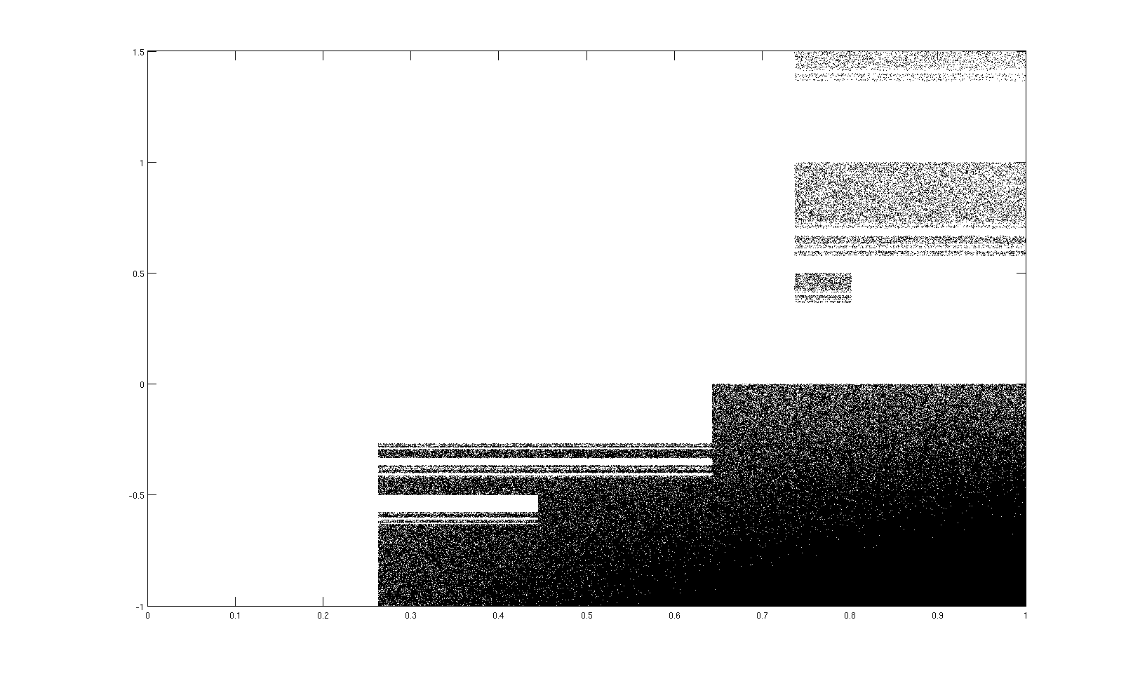
(a) $\alpha\approx 0.73694949$

(b) $\alpha\approx 0.79347519$

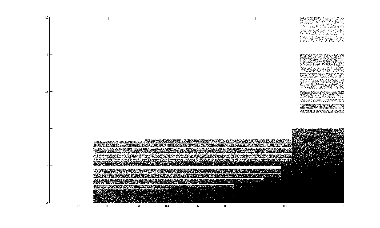
(c) $\alpha\approx 0.85019348$

(d) $\alpha\approx 0.89348572$

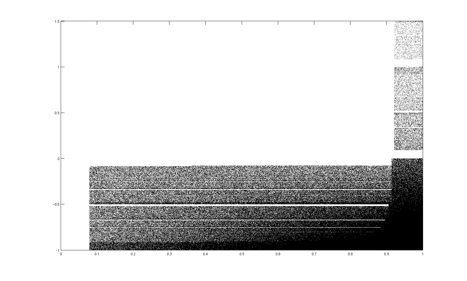
(e) $\alpha\approx 0.92087668$

(f) $\alpha\approx 0.95234649$

Figure 4. Numerical simulations of $\mathcal{D}_{\alpha}$ for $\alpha>\frac{1}{2}\sqrt{2}$.

5. Entropy, wandering rate and isomorphisms

With an explicit expression for the density of $\mu_{\alpha}$ at hand, we can compute several dynamical quantities associated to the systems $T_{\alpha}$. In this section we compute the Krengel entropy, return sequence and wandering rate of $T_{\alpha}$ for a large part of the parameter space $(0,1)$.

In [Kre67] Krengel extended the notion of metric entropy to infinite, measure preserving and conservative systems $(X,\mathcal{B},\mu,T)$ by considering the metric entropy on finite measure induced systems. More precisely, if $A$ is a sweep-out set for $T$ with $\mu(A)<\infty$, $T_{A}$ the induced transformation of $T$ on $A$ and $\mu_{A}$ the restriction of $\mu$ to $A$, then the Krengel entropy of $T$ is defined to be

$$h_{\text{Kr},\mu}(T)=h_{\mu_{A}}(T_{A},\mu_{A}),$$

where $h_{\mu_{A}}(T_{A},\mu_{A})$ is the metric entropy of the system $(A,\mathcal{B}\cap A,T_{A},\mu_{A})$. Krengel proved in [Kre67] that this quantity is independent of the choice of $A$. In [Zwe00, Theorem 6] it is shown that if $T$ is an AFN-map the Krengel entropy can be computed using Rohlin’s formula:

(16) $$h_{\text{Kr},\mu}(T)=\int_{X}\log(|T^{\prime}|)d\mu.$$

The following theorem follows from Lemma 2.2, (15) and Table 1.

Theorem 5.1.

For any $\alpha\in\big{(}0,g\big{]}$ the system $(I_{\alpha},\mathcal{B}_{\alpha},\mu_{\alpha},T_{\alpha})$ has $h_{\text{Kr},\mu_{\alpha}}(T_{\alpha})=\frac{\pi^{2}}{6}$.

Proof.

First fix $\alpha\in\big{(}0,\frac{1}{2}\big{)}$. By Lemma 2.2 we can use formula (16) to compute the Krengel entropy of $T_{\alpha}$. For this computation we use some properties of the dilogarithm function, which is defined by

$$\operatorname{Li}_{2}(x):=\sum_{n=1}^{\infty}\frac{x^{n}}{n^{2}}\quad\text{ for }|x|\leq 1,$$

and satisfies (see [Lew81] for more information)

• $\operatorname{Li}_{2}(0)=0$;

• $\operatorname{Li}_{2}(-1)=-\pi^{2}/12$;

• $\operatorname{Li}_{2}(x)+\operatorname{Li}_{2}(-\frac{x}{1-x})=-\frac{1}{2}\log^{2}(1-x)$.

Using the density from (15) and these three properties of $\operatorname{Li}_{2}$ we get

$$\int_{I_{\alpha}}\log(|T^{\prime}_{\alpha}|)d\mu_{\alpha} =-2\bigg{(}\int_{\alpha}^{\frac{\alpha}{1-\alpha}}\frac{\log x}{x}dx+\int_{\frac{\alpha}{1-\alpha}}^{1-\alpha}\frac{\log x}{1+x}dx+2\int_{1-\alpha}^{1}\frac{\log x}{1-x^{2}}dx\bigg{)}$$

$$=[-\log^{2}x]_{\alpha}^{\frac{\alpha}{1-\alpha}}-2[\operatorname{Li}_{2}(-x)+\log x\log(x+1)]_{\frac{\alpha}{1-\alpha}}^{1-\alpha}$$

$$\quad-2[\operatorname{Li}_{2}(1-x)+\operatorname{Li}_{2}(-x)+\log x\log(x+1)]_{1-\alpha}^{1}$$

$$=-\log^{2}\Big{(}\frac{\alpha}{1-\alpha}\Big{)}+\log^{2}(\alpha)+2\operatorname{Li}_{2}\Big{(}\frac{-\alpha}{1-\alpha}\Big{)}+2\log\Big{(}\frac{\alpha}{1-\alpha}\Big{)}\log\Big{(}\frac{1}{1-\alpha}\Big{)}$$

$$\quad-2\operatorname{Li}_{2}(-1)+2\operatorname{Li}_{2}(\alpha)$$

$$=\log^{2}(\alpha)-\log^{2}\big{(}\frac{\alpha}{1-\alpha}\big{)}-\log^{2}(1-\alpha)-2\log\big{(}\frac{\alpha}{1-\alpha}\big{)}\log(1-\alpha)+\frac{\pi^{2}}{6}$$

$$=\log^{2}(\alpha)-\log^{2}(\alpha)+2\log(\alpha)\log(1-\alpha)-2\log^{2}(1-\alpha)+$$

$$\quad-2\log(\alpha)\log(1-\alpha)+2\log^{2}(1-\alpha)+\frac{\pi^{2}}{6}$$

$$=\frac{\pi^{2}}{6}.$$

A similar computation yields $h_{\text{Kr},\mu_{\alpha}}(T_{\alpha})=\frac{\pi^{2}}{6}$ for $\alpha\in[\frac{1}{2},g]$. ∎

Remark 5.2.

Numerical evidence using the densities from Table 1 suggests that $h_{\text{Kr},\mu_{\alpha}}(T_{\alpha})=\frac{\pi^{2}}{6}$ for $\alpha\in(g,\frac{1}{2}\sqrt{2})$ as well. Even though we were not able to calculate the Krengel entropy for $\alpha\in(g,\frac{1}{2}\sqrt{2})$ explicitly, we conjecture that in fact $h_{\text{Kr},\mu_{\alpha}}(T_{\alpha})=\frac{\pi^{2}}{6}$ for all $\alpha\in(0,1)$. This claim is supported by the fact that the Krengel entropy for Nakada’s $\alpha$-continued fraction maps $S_{\alpha}$ from (2) is $\frac{\pi^{2}}{6}$ as well, see [KSS12, Theorem 2].

The return sequence of $T_{\alpha}$ is the sequence $(a_{n}(T_{\alpha}))_{n\geq 1}$ of positive real numbers satisfying (7). The pointwise dual ergodicity of each map $T_{\alpha}$ implies that such a sequence, which is unique up to asymptotic equivalence, exists. The asymptotic type of $T_{\alpha}$ corresponds to the family of all sequences asymptotically equivalent to some positive multiple of $(a_{n}(T_{\alpha}))_{n\geq 1}$. The return sequence of a system is related to its wandering rate, which quantifies how big the system is in relation to its subsets of finite measure. To be more precise, if $(X,\mathcal{B},\mu,T)$ is a conservative, ergodic, measure preserving system and $A\in\mathcal{B}$ a set of finite positive measure, then the wandering rate of $A$ with respect to $T$ is the sequence $(w_{n}(A))_{n\geq 1}$ given by

$$w_{n}(A):=\mu\bigg{(}\bigcup_{k=0}^{n-1}T^{-k}A\bigg{)}.$$

It follows from [Zwe00, Theorem 2] that for each of the maps $T_{\alpha}$ there exists a positive sequence $(w_{n}(T_{\alpha}))$ such that $w_{n}(T_{\alpha})\uparrow\infty$ and $w_{n}(T_{\alpha})\sim w_{n}(A)$ as $n\to\infty$ for all sets $A$ that have positive, finite measure and are bounded away from 1. The asymptotic equivalence class of $(w_{n}(T_{\alpha}))$ defines the wandering rate of $T_{\alpha}$. Using the machinery from [Zwe00] and the explicit formula of the density we compute both the return sequence and the wandering rate of the maps $T_{\alpha}$.

Proposition 5.3.

For all $\alpha\in(0,1)$ there is a constant $c_{\alpha}>0$ such that

$$w_{n}(T_{\alpha})\sim c_{\alpha}\log n\quad\textit{and}\quad a_{n}(T_{\alpha})\sim\frac{n}{c_{\alpha}\log n}.$$

If $\alpha\in(0,\frac{1}{2}\sqrt{2})$, then $c_{\alpha}=1$.

Proof.

Using the Taylor expansion of the maps $T_{\alpha}$, one sees that for $x\rightarrow 1$ we have $T_{\alpha}(x)=x-(x-1)^{2}+o((x-1)^{2})$. Hence, $T_{\alpha}$ admits what are called nice expansions in [Zwe00]. For $x\in\big{(}\frac{1}{1+\alpha},1\big{]}$ we can write $f_{\alpha}(x)=\frac{x-2}{x-1}H(x)$, where the function $x\mapsto\frac{x-2}{x-1}$ corresponds to the map called $G$ in [Zwe00, Theorem A]. It then follows by [Zwe00, Theorems 3 and 4] that the wandering rate is

(17) $$w_{n}(T_{\alpha})\sim c_{\alpha}\log n$$

and the return sequence is

(18) $$a_{n}(T_{\alpha})\sim\frac{n}{c_{\alpha}\log n},$$

for $c_{\alpha}=\lim_{x\uparrow 1}H(x)$. For $\alpha\in\big{(}0,\frac{1}{2}\sqrt{2}\big{)}$ the explicit formula for the densities from (15) and Table 1 gives $c_{\alpha}=1$. ∎

We have now established all parts of Theorem 1.2.

Proof of Theorem 1.2.

The densities are given by (15) and listed in Table 1. The entropy is given by Theorem 5.1 and the wandering rate and return sequence in Proposition 5.3. ∎

Remark 5.4.

(i) As in Remark 5.2 we suspect that in fact $c_{\alpha}=1$ for all $\alpha\in(0,1)$.

(ii) Since all the results from [Zwe00] apply to our family, we can use these to get an even more detailed description of the ergodic behaviour of the maps $T_{\alpha}$. We briefly mention a few more results for $\alpha\in(0,1/2\sqrt{2}]$. Since the return sequence $(a_{n}(T_{\alpha}))_{n\geq 1}$ is regularly varying with index $1$, by [Zwe00, Theorem 5] and [Aar97, Corollary 3.7.3], we have

(19) $$\frac{\log n}{n}\sum_{k=0}^{n-1}f\circ T_{\alpha}^{k}\xrightarrow{\mu_{\alpha}}\int_{I_{\alpha}}f\,d\mu_{\alpha},\quad\text{ for }f\in L^{1}(I_{\alpha},\mathcal{B}_{\alpha},\mu_{\alpha})\text{ and }\int_{I_{\alpha}}f\,d\mu_{\alpha}\neq 0.$$

In other words, a weak law of large numbers holds for $T_{\alpha}$.

In addition, we can obtain asymptotics for the excursion times to the interval $\big{[}\frac{1}{1+\alpha},1\big{]}$, corresponding to the rightmost branch of $T_{\alpha}$. Let $Y$ be a sweep-out set, $T_{Y}$ the induced map on $Y$ and $\varphi:x\mapsto\min\{n\geq 1:T^{n}(x)\in Y\}$ the first return map. Write $\varphi_{n}^{Y}:=\sum_{k=0}^{n-1}\varphi\circ T_{Y}^{k}$ and note that the asymptotic inverse of the sequence $(a_{n}(T_{\alpha}))_{n\geq 1}$ is $(n\log n)_{n\geq 1}$, so that the statement from (19) is equivalent to the following dual:

$$\frac{1}{n\log n}\varphi_{n}^{Y}\xrightarrow{\mu_{\alpha}}\frac{1}{\mu_{\alpha}(Y)}.$$

If we induce on $Y:=\big{[}\min\{\alpha,1-\alpha\},\frac{1}{1+\alpha}\big{]}$, then $\varphi_{n}^{Y}$ sums the lengths (increased by $n$) of the first $n$ blocks of consecutive digits $(\epsilon,d)=(-1,2)$, and we obtain

$$\frac{1}{n\log n}\varphi_{n}^{Y}-\frac{1}{\log n}\xrightarrow{\mu_{\alpha}}\frac{1}{\mu_{\alpha}(Y)}.$$

From Theorem 1.2, it follows that for $\alpha<\frac{1}{2}$, $\mu_{\alpha}(Y)=\log(2+\alpha)$. Note that for $\alpha$ decreasing the right hand side is increasing, meaning we spend on average more time in $\Delta(-1,2)$. Intuitively, for a smaller $\alpha$, every time we enter $\Delta(-1,2)$ we are closer to the indifferent fixed point, and it takes longer before we manage to escape from it.

Note that the Krengel entropy, return sequence and wandering rate we found do not display any dependence on $\alpha$. These quantities give isomorphism invariants for dynamical systems with infinite invariant measures. Two measure preserving dynamical systems $(X,\mathcal{B},\mu,T)$ and $(Y,\mathcal{C},\nu,S)$ on $\sigma$-finite measure spaces are called $c$-isomorphic for $c\in(0,\infty]$ if there are sets $N\in\mathcal{B}$, $M\in\mathcal{C}$ with $\mu(N)=0=\nu(M)$ and $T(X\setminus N)\subseteq X\setminus N$ and $S(Y\setminus M)\subseteq Y\setminus M$ and if there is a map $\phi:X\setminus N\to Y\setminus M$ that is invertible, bi-measurable and satisfies $\phi\circ T=S\circ\phi$ and $\mu\circ\phi^{-1}=c\cdot\nu$. Invariants for $c$-isomorphisms are the asymptotic proportionality classes of the return sequence (see [Aar97, Propositions 3.7.1 and 3.3.2] and [Zwe00, Remark 8]) and the normalised wandering rates, which combine the Krengel entropy with the wandering rates (see e.g. [Tha83, Zwe00]). It follows from Theorem 1.2 that all these quantities are equal for all $T_{\alpha}$, $\alpha\in(0,\frac{1}{2}\sqrt{2})$. Using the idea from [Kal14], however, we find many pairs $\alpha$ and $\alpha^{\prime}$ such that $T_{\alpha}$ and $T_{\alpha^{\prime}}$ are not $c$-isomorphic for any $c\in(0,\infty]$. Consider for example any $\alpha\in\big{(}\sqrt{2}-1,\frac{1}{2}\big{)}$, so that $\alpha\in\big{(}\frac{1}{2+\alpha},\frac{1}{2}\big{)}$, and any $\alpha^{\prime}\in\big{(}\frac{1}{3},\frac{3-\sqrt{5}}{2}\big{)}$, so that $T_{\alpha^{\prime}}(\alpha^{\prime})>1-\alpha^{\prime}$, see Figure 5. For a contradiction, suppose that there is a $c$-isomorphism $\phi:I_{\alpha}\to I_{\alpha^{\prime}}$ for some $c\in(0,\infty]$. Let $J=[\alpha,1-\alpha]$ and note that any $x\in J$ has precisely one pre-image under $T_{\alpha}$. Since $\phi\circ T_{\alpha}=T_{\alpha^{\prime}}\circ\phi$ and $\phi$ is invertible, any element of the set $\phi(J)$ must also have precisely one pre-image. Since $T_{\alpha^{\prime}}(\alpha^{\prime})>1-\alpha^{\prime}$, there are no such points, so $\mu_{\alpha^{\prime}}(\phi(J))=0$. On the other hand, since $J$ is bounded away from 1, it follows that $0<\mu_{\alpha}(J)<\infty$. Hence, there can be no $c$, such that $\mu_{\alpha^{\prime}}\circ\phi^{-1}=c\cdot\mu_{\alpha}$. Obviously a similar argument holds for many other combinations of $\alpha$ and $\alpha^{\prime}$, even for $\alpha>\frac{1}{2}$, and in case the argument does not work for $T_{\alpha}$ and $T_{\alpha^{\prime}}$, one can also consider iterates $T_{\alpha}^{n}$, $T_{\alpha^{\prime}}^{n}$. Hence, even though the above discussed isomorphism invariants are equal for all $\alpha\in\big{(}0,\frac{1}{2}\big{)}$, it is not generally the case that any two maps $T_{\alpha}$ are $c$-isomorphic. We conjecture that for almost all pairs $(\alpha,\alpha^{\prime})$, the maps $T_{\alpha}$ and $T_{\alpha^{\prime}}$ are not $c$-isomorphic.

(a) $\alpha\in\big{(}\sqrt{2}-1,\frac{1}{2}\big{)}$

(b) $\alpha^{\prime}\in\big{(}\frac{1}{3},\frac{3-\sqrt{5}}{2}\big{)}$

Figure 5. Maps $T_{\alpha}$ and $T_{\alpha^{\prime}}$ that are not $c$-isomorphic for any $c\in\mathbb{(}0,\infty]$.

6. Acknowledgment

The third author is supported by the NWO TOP-Grant No. 614.001.509.

References

- [Aar97] J. Aaronson. An introduction to infinite ergodic theory, volume 50 of Mathematical Surveys and Monographs. American Mathematical Society, Providence, RI, 1997.
- [AS13] P. Arnoux and T. A. Schmidt. Cross sections for geodesic flows and -continued fractions. Nonlinearity, 26(3):711–726, 2013.
- [BCIT13] C. Bonanno, C. Carminati, S. Isola, and G. Tiozzo. Dynamics of continued fractions and kneading sequences of unimodal maps. Discrete Contin. Dyn. Syst., 33(4):1313–1332, 2013.
- [BCK17] H. Bruin, C. Carminati, and C. Kalle. Matching for generalised -transformations. Indag. Math. (N.S.), 28(1):55–73, 2017.
- [BCMP18] H. Bruin, C. Carminati, S. Marmi, and A. Profeti. Matching in a family of piecewise affine maps. Nonlinearity, 32(1):172–208, 2018.
- [BSORG13] V. Botella-Soler, J. A. Oteo, J. Ros, and P. Glendinning. Lyapunov exponent and topological entropy plateaus in piecewise linear maps. J. Phys. A, 46(12):125101, 26, 2013.
- [CIT18] C. Carminati, S. Isola, and G. Tiozzo. Continued fractions with -branches: combinatorics and entropy. Trans. Amer. Math. Soc., 370(7):4927–4973, 2018.
- [CM18] D. Cosper and M. Misiurewicz. Entropy locking. Fund. Math., 241(1):83–96, 2018.
- [CMPT10] C. Carminati, S. Marmi, A. Profeti, and G. Tiozzo. The entropy of -continued fractions: numerical results. Nonlinearity, 23(10):2429–2456, 2010.
- [CT12] C. Carminati and G. Tiozzo. A canonical thickening of and the entropy of -continued fraction transformations. Ergodic Theory Dynam. Systems, 32(4):1249–1269, 2012.
- [CT13] C. Carminati and G. Tiozzo. Tuning and plateaux for the entropy of -continued fractions. Nonlinearity, 26(4):1049–1070, 2013.
- [DHKM12] K. Dajani, D. Hensley, C. Kraaikamp, and V. Masarotto. Arithmetic and ergodic properties of ‘flipped’ continued fraction algorithms. Acta Arith., 153(1):51–79, 2012.
- [DK00] K. Dajani and C. Kraaikamp. The mother of all continued fractions. Colloq. Math., 84/85(part 1):109–123, 2000. Dedicated to the memory of Anzelm Iwanik.
- [DK17] K. Dajani and C. Kalle. Invariant measures, matching and the frequency of 0 for signed binary expansions. arXiv: 1703.06335, 2017.
- [DKS09] K. Dajani, C. Kraaikamp, and W. Steiner. Metrical theory for -Rosen fractions. J. Eur. Math. Soc. (JEMS), 11(6):1259–1283, 2009.
- [Haa02] Andrew Haas. Invariant measures and natural extensions. Canad. Math. Bull., 45(1):97–108, 2002.
- [HK02] Y. Hartono and C. Kraaikamp. On continued fractions with odd partial quotients. Rev. Roumaine Math. Pures Appl., 47(1):43–62 (2003), 2002.
- [Kal14] C. Kalle. Isomorphisms between positive and negative -transformations. Ergodic Theory Dynam. Systems, 34(1):153–170, 2014.
- [Kra91] C. Kraaikamp. A new class of continued fraction expansions. Acta Arith., 57(1):1–39, 1991.
- [Kre67] U. Krengel. Entropy of conservative transformations. Z. Wahrscheinlichkeitstheorie und Verw. Gebiete, 7:161–181, 1967.
- [KS12] C. Kalle and W. Steiner. Beta-expansions, natural extensions and multiple tilings associated with Pisot units. Trans. Amer. Math. Soc., 364(5):2281–2318, 2012.
- [KSS12] C. Kraaikamp, T. Schmidt, and W. Steiner. Natural extensions and entropy of -continued fractions. Nonlinearity, 25(8):2207–2243, 2012.
- [KU10] S. Katok and I. Ugarcovici. Structure of attractors for -continued fraction transformations. J. Mod. Dyn., 4(4):637–691, 2010.
- [Lew81] L. Lewin. Polylogarithms and associated functions. North-Holland Publishing Co., New York-Amsterdam, 1981.
- [LM08] L. Luzzi and S. Marmi. On the entropy of Japanese continued fractions. Discrete Contin. Dyn. Syst., 20(3):673–711, 2008.
- [MMY97] S. Marmi, P. Moussa, and J.C. Yoccoz. The Brjuno functions and their regularity properties. Comm. Math. Phys., 186(2):265–293, 1997.
- [Nak81] H. Nakada. Metrical theory for a class of continued fraction transformations and their natural extensions. Tokyo J. Math., 4(2):399–426, 1981.
- [NN08] H. Nakada and R. Natsui. The non-monotonicity of the entropy of -continued fraction transformations. Nonlinearity, 21(6):1207–1225, 2008.
- [Per57] O. Perron. Die Lehre von den Kettenbrüchen. Dritte, verbesserte und erweiterte Aufl. Bd. II. Analytisch-funktionentheoretische Kettenbrüche. B. G. Teubner Verlagsgesellschaft, Stuttgart, 1957.
- [Roh61] V. A. Rohlin. Exact endomorphisms of a Lebesgue space. Izv. Akad. Nauk SSSR Ser. Mat., 25:499–530, 1961.
- [Sch04] B. Schratzberger. -expansions in dimension two. J. Théor. Nombres Bordeaux, 16(3):705–732, 2004.
- [Sil88] C. E. Silva. On -recurrent nonsingular endomorphisms. Israel J. Math., 61(1):1–13, 1988.
- [ST91] C. E. Silva and P. Thieullen. The subadditive ergodic theorem and recurrence properties of Markovian transformations. J. Math. Anal. Appl., 154(1):83–99, 1991.
- [Tha83] M. Thaler. Transformations on with infinite invariant measures. Israel J. Math., 46(1-2):67–96, 1983.
- [Tio14] G. Tiozzo. The entropy of Nakada’s -continued fractions: analytical results. Annali della Scuola Normale Superiore di Pisa, 13(4):1009–1037, 2014.
- [Zwe00] R. Zweimüller. Ergodic properties of infinite measure-preserving interval maps with indifferent fixed points. Ergodic Theory Dynam. Systems, 20(5):1519–1549, 2000.