Intelligent Reflecting Surface-Assisted Cognitive Radio System

Abstract

Cognitive radio (CR) is an effective solution to improve the spectral efficiency (SE) of wireless communications by allowing the secondary users (SUs) to share spectrum with primary users. Meanwhile, intelligent reflecting surface (IRS), also known as reconfigurable intelligent surface (RIS), has been recently proposed as a promising approach to enhance energy efficiency (EE) of wireless communication systems through intelligently reconfiguring the channel environment. To improve both SE and EE, in this paper, we introduce multiple IRSs to a downlink multiple-input single-output (MISO) CR system, in which a single SU coexists with a primary network with multiple primary user receivers (PU-RXs). Our design objective is to maximize the achievable rate of SU subject to a total transmit power constraint on the SU transmitter (SU-TX) and interference temperature constraints on the PU-RXs, by jointly optimizing the beamforming at SU-TX and the reflecting coefficients at each IRS. Both perfect and imperfect channel state information (CSI) cases are considered in the optimization. Numerical results demonstrate that the introduction of IRS can significantly improve the achievable rate of SU under both perfect and imperfect CSI cases.

I Introduction

By the year 2020, wireless communication is expected to serve approximately $50$ billion devices and each person will be surrounded by more than six devices on average [ericsson2011more]. This will lead to tremendous solicitation of radio resources including bandwidth and energy. Therefore, spectral efficiency (SE) and energy efficiency (EE) are becoming two essential criteria for designing future wireless networks [JoHoSu14JSAC].

Cognitive radio (CR) has been proposed as an effective technique to enhance the SE [mitola1999cognitive, haykin2005cognitive]. Specifically, a spectrum sharing-based CR network allows secondary users (SUs) to share the spectrum with primary users (PUs) while controlling the interference leakage to PU receivers (PU-RXs). One design strategy is to maximize the achievable rates of SUs, while sustaining the interference temperature (IT) at PU-RXs below a certain threshold [haykin2005cognitive]. The threshold in the IT constraint is evidently designed to ensure that the presence of SUs incurs an acceptable degradation in the quality-of-service (QoS) of the PUs. Under this circumstance, the beamforming technique is generally recognized as an effective means to support the optimal transmission scheme [cumanan2009sinr, yiu2008interference]. In practice, the CSI obtained by the SU-TX could be imperfect owing to inevitable practical issues, such as channel estimation errors, quantization errors, and outdated information due to feedback delay. To circumvent this issue, the robust beamforming design has been studied to explicitly take into account those errors [zheng2010robust, gong2013robust, suraweera2010capacity, kang2011optimal, rezki2012ergodic, xiong2015robust].

On the other hand, intelligent reflection surface (IRS), also known as reconfigurable intelligent surface (RIS), has recently attracted considerable attention from the research community of wireless communications for its ability to improve EE [nature18, cui2014coding, BaReRoDeAlZh19, huang2019reconfigurable, liang2019large]. The IRS is an artificial surface made of electromagnetic material that consists of a large number of passive and low-cost reflecting elements [nature18, cui2014coding, BaReRoDeAlZh19, liang2019large], which introduce phase shifts and amplitude variations of the incident signals. By doing so, the incident electromagnetic wave can be directed to the desired directions [BaReRoDeAlZh19, huang2019reconfigurable]. Similar to the cooperative relaying systems [ngo2014multipair, JoCh19], IRS can construct additional wireless links, yet it does not require active radio frequency components. Besides, owing to the passive structure, there is nearly no additional power consumption and added thermal noise during reflection. On the other hand, compared to backscatter communication [yang2017modulation, XiGuLi19, liang2019large], the IRS aims to assist the transmission of the intended wireless network without attempting its own information transmission.

Motivated by the inspiration of CR and IRS, in this paper, we propose an IRS-assisted downlink MISO CR network to enhance both SE and EE. As shown in Fig. 1, generalizing from a single IRS scenario [YuLiJoFeLa19], multiple IRSs are deployed to assist the CR network, in which a SU transmitter (SU-TX) with multiple antennas communicates with a single-antenna SU-RX and shares the same spectrum with several PUs. Our objective is to jointly optimize the beamforming vector at SU-TX and the reflecting coefficients at each IRS for the IRS-assisted CR system to maximize the achievable rate of SU subject to a total power constraint on SU-TX and IT constraints on PU-RXs. Both perfect CSI and imperfect CSI cases are considered. The main contributions of this paper are summarized as follows:

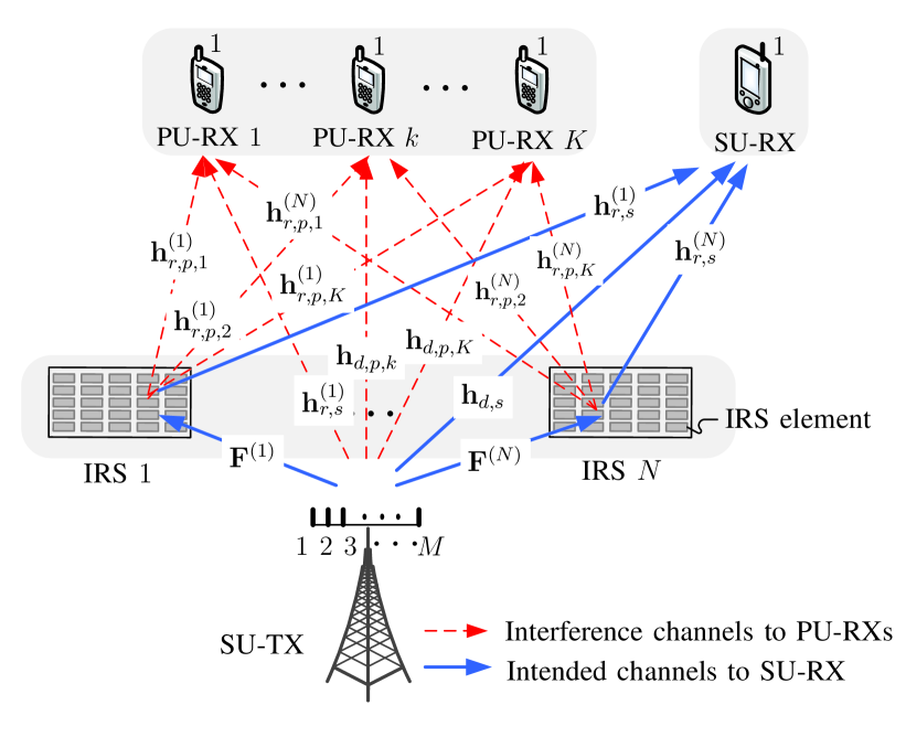
Figure 1: IRS-assisted downlink MISO CR network model with one pair of SU-TX and SU-RS, $N$ IRSs, and $K$ PU-RXs.

• We formulate a SU rate maximization problem by optimizing the transmit beamforming vector at the SU-TX and reflecting coefficients at each IRS. Both transmit power constraint at SU-TX and interference temperature constraints at PUs are considered.

• For perfect CSI case, an efficient iterative algorithm based on the block coordinate descent (BCD) method [wright2015coordinate] is proposed. In each iteration, first, the beamforming vector at the SU-TX is optimized by solving a second order cone programming (SOCP). Then, the reflecting coefficients are optimized by applying the semidefinite relaxation (SDR) technique to relax the rank-$1$ constraint on the reflecting coefficient matrices. Later, the Gaussian randomization scheme proposed in [992139] is used to recover the rank-$1$ variables.

• For imperfect CSI case, the worst case approach is used, in which the channel uncertainty is modelled by a given ellipsoid region [zheng2009robust, wang2009worst]. With that, the formulated problem is transformed to the worst-case robust optimization problem, i.e., a maxmin problem. The SDR technique is again used to relax the rank-$1$ constraints of the optimization problem. Then, we transform the maxmin problem to a maximization problem, and the variables are alternatively updated by decoupling the original problem into two subproblems. In each subproblem, using the $\mathcal{S}$-Procedure [beck2006strong], the equivalent IT and signal-to-noise ratio (SNR) constraints can be derived.

The remaining parts of this paper are organized as follows. Section II presents a brief overview of the related work. The system model of IRS-assisted CR system and the problem formulation are introduced in Section III. Section IV addresses the perfect CSI case and decouples the original problem into an SOCP subproblem and a semidefinite programming (SDP) subproblem. Section IV is devoted to the imperfect CSI case, in which we formulate the worst-case optimization problem and then propose an alternating optimization method to solve it. Numerical results to evaluate the performance of the proposed system are provided and discussed in Section LABEL:sec:simulations. Section LABEL:sec:conclusion concludes this paper.

Notations: The scalars, column vectors, and matrices are denoted by a lower case, boldface lower case, and boldface upper case letters, respectively, i.e., $a$, $\mathbf{a}$, and $\mathbf{A}$. For vector ${\bf a}$, ${\rm diag}({\bf a})$ gives a diagonal matrix whose diagonal elements correspond to ${\bf a}$ and $[{\bf a}]_{i}$ means the $i$th element of ${\bf a}$. For matrix $\mathbf{A}$, $\mathrm{tr}(\mathbf{A})$, $\|\mathbf{A}\|$, $\mathrm{rank}(\mathbf{A})$, $\mathbf{A}^{T}$, $\mathbf{A}^{\dagger}$, and $[\mathbf{A}]_{i,j}$ denote its trace, Frobenius norm, rank, transpose, complex conjugate transpose, and the $(i,j)$th element, respectively. $\mathbf{A}\succeq 0$ means that $\mathbf{A}$ is a positive semidefinite (PSD) matrix. $\mathbf{A}\otimes\mathbf{B}$ denotes the Kronecker product of $\mathbf{A}$ and $\mathbf{B}$. $\mathrm{vec}(\mathbf{A})$ is a column vector by stacking all the elements of $\mathbf{A}$. $\mathcal{CN}(\mu,\sigma^{2})$ denotes the distribution of a circularly symmetric complex Gaussian random variable with mean $\mu$ and variance $\sigma^{2}$. $\mathbf{0}_{N}$ and $\mathbf{I}_{N}$ denote the $N$-dimensional zero and identity matrices, respectively.

II Related Work

In this section, we conduct a brief survey for the related work in three aspects, which includes CR beamforming, robust beamforming, and IRS-assisted wireless communication system.

II-1 CR Beamforming

So far, a lot of CR beamforming techniques have been designed by assuming that the CSI is perfectly known at SU-TX [zhang2008exploiting, cumanan2009sinr, tajer2009beamforming, islam2008joint, yiu2008interference]. Specifically, in [zhang2008exploiting], a single SU is considered for spectrum sharing by restricting the interference leakages to each PU. For multiple SUs, beamforming techniques are proposed to maximize the minimum signal-to-interference-plus-noise ratio (SINR) and the minimum rate of SUs in [cumanan2009sinr] and [tajer2009beamforming], respectively. In [islam2008joint], centralized joint beamforming and power control methods are studied for multiple SUs with multiple antennas. The beamforming designed in [yiu2008interference] maximizes the ratio between the received signal power at SUs and the interference leakage to PUs.

II-2 Robust Beamforming

Robust beamforming techniques that tackle the channel uncertainty have been addressed in many studies, and the main techniques fall into two categories. One is the stochastic approach, in which the CSI errors are modeled as Gaussian random variables and the parametric constraints are modeled by the probability constraints [zheng2010robust, gong2013robust, suraweera2010capacity, kang2011optimal, rezki2012ergodic, xiong2015robust]. The other one is the worst-case approach, in which the CSI errors are assumed to be within a given uncertainty set and the optimization is performed under the worst-case channel condition [zhang2009robust, zhang2012distributed, cumanan2008robust, wang2014robust, pei2011secure]. Specifically, in [zhang2009robust, zhang2012distributed], only the CSI uncertainty in primary link is considered for multiple-input single-output (MISO) and multiple-input multiple-output (MIMO) CR network. Considering the CSI uncertainty in both primary and secondary links, the worst-case robust design is used to minimize the total transmit power in [cumanan2008robust], maximize the robust EE in [wang2014robust], and maximize the achievable secrecy-rate in [pei2011secure].

II-3 IRS-assisted Wireless Communication System

Owing to the promising features of IRS, IRS-assisted wireless communication systems have been vigorously studied recently [yang2019irs, li2019reconfigurable, chen2019intelligent, yu2019enabling, mishra2019channel, yang2019intelligent, wu2019intelligent, guo2019weighted, NaKaChDeAl19, huang2018energy, huang2019reconfigurable, han2019large]. Specifically, the achievable rate maximization problem is studied in [yang2019irs] for orthogonal frequency division multiplexing (OFDM) systems. The unmanned aerial vehicle (UAV) trajectory is designed for IRS-assisted UAV system to maximize the average achievable rate [li2019reconfigurable]. The physical layer security problem is considered in [chen2019intelligent] and [yu2019enabling]. The minimum-secrecy-rate maximization problem is studied in [chen2019intelligent] which considers both continuous and discrete reflecting coefficients. The IRS-assisted transmit beamforming is designed in [mishra2019channel] to support wireless power transfer. The IRS-assisted non-orthogonal-multiple access system is considered in [yang2019intelligent], in which a base station (BS) transmits superimposed downlink signals to multiple users. For multiuser MISO communication systems, the IRS is exploited to enhance the weighted sum-rate in [wu2019intelligent], [guo2019weighted], or maximize the minimum SINR in [NaKaChDeAl19]. EE is improved by using transmit power allocation and designing the reflecting coefficients of the IRS aided by precoding [huang2018energy, huang2019reconfigurable]. The impact of phase shift on the ergodic SE is investigated in [han2019large] by exploiting the statistical CSI.

However, there is no related work that introduces multiple IRSs into CR networks while considering both perfect and imperfect CSI cases.

III System Model

As shown in Fig. 1, we consider an IRS-assisted CR downlink network with $N(N\geq 1)$ IRSs, $K$ ($K\geq 1$) PU-RXs, and a pair of SU-TX and SU-RX. The SU-TX has $M$ transmit antennas, while each RX has a single receive antenna. We assume that the SU uses the same frequency band as the PUs, and each IRS is composed of $L$ ($L>1$) passive reflecting elements, through which the impinging electromagnetic wave is directed to a desired direction.

III-A Channel Model

We denote the baseband equivalent direct-link channel responses from the SU-TX to PU-RXs and SU-RX by $\mathbf{h}_{d,p,k}\in\mathbb{C}^{M\times 1}$ for $k\in\mathcal{K}=\{1,\ldots,K\}$ and $\mathbf{h}_{d,s}\in\mathbb{C}^{M\times 1}$, respectively, where each element of $\mathbf{h}_{d,p,k}$ and $\mathbf{h}_{d,s}$ is an independent and identically distributed (i.i.d.) complex Gaussian random variable with a zero mean and unit variance, namely, $\mathbf{h}_{d,p,k}\sim\mathcal{CN}({\bf 0}_{M},{\bf I}_{M})$ and $\mathbf{h}_{d,s}\sim\mathcal{CN}({\bf 0}_{M},{\bf I}_{M})$, respectively. The baseband equivalent channel responses from the SU-TX to the $n$th IRS is denoted by $\mathbf{F}^{(n)}\in\mathbb{C}^{L\times M}$ for $n\in\mathcal{N}=\{1,\ldots,N\}$. In reality, the IRSs are envisioned to be deployed on the facade of a building close to the BS and users; therefore, we can assume that a line of sight (LoS) path exists in the reflect-link. Therefore, the channel $\mathbf{F}^{(n)}$ can be modeled as a Rician fading channel as follows:

$$\mathbf{F}^{(n)}=\sqrt{\frac{\kappa_{1}}{\kappa_{1}+1}}\mathbf{F}^{{(n)},\rm LoS}+\sqrt{\frac{1}{\kappa_{1}+1}}\mathbf{F}^{{(n)},\rm NLoS},$$ (1)

where $\kappa_{1}$ is the Rician factor and $\mathbf{F}^{{(n)},\rm LoS}\in\mathbb{C}^{L\times M}$ represents the fixed channel related to the LoS component, while $\mathbf{F}^{{(n)},\rm NLoS}\in\mathbb{C}^{L\times M}$ represents the NLoS channel matrix, whose elements are i.i.d. that conform to the complex Gaussian distribution with a zero mean and unit variance.

In (1), ${\bf F}^{{(n)},\rm LoS}$ is precisely modeled as

$$\mathbf{F}^{{(n)},\rm LoS}=\mathbf{a}_{L}\left(\beta^{(n)}_{\mathrm{AoA}}\right)\left(\mathbf{a}_{M}\left(\beta^{(n)}_{\mathrm{AoD}}\right)\right)^{\dagger},$$ (2)

where $\beta^{(n)}_{\mathrm{AoA}}$ and $\beta^{(n)}_{\mathrm{AoD}}$ denote the angle of arrival (AoA) and angle of departure (AoD) of IRS $n$, respectively. Here, $\mathbf{a}_{q}(\beta)\in\mathbb{C}^{q\times 1}$ is a $q$-dimension uniform linear array response vector given as follows:

$$\mathbf{a}_{q}(\beta)=\left[1,e^{j\frac{2{\pi}d}{\lambda}\sin(\beta)},e^{j\frac{4{\pi}d}{\lambda}\sin(\beta)},\ldots,e^{j\frac{2(q-1){\pi}d}{\lambda}\sin(\beta)}\right]^{T},$$ (3)

where $\beta$ is the angle, $d$ is the distance between adjacent IRS elements, and $\lambda$ denotes the wavelength of the carrier. To remove the ambiguity in AoA estimation within the AoA interval, we set $d/\lambda$ to be $1/2$.

Likewise, the channels of reflect-link from IRS $n$ to PU-RX $k$ and SU-RX are denoted by $\mathbf{h}^{(n)}_{r,p,k}\in\mathbb{C}^{L\times 1}$ and $\mathbf{h}^{(n)}_{r,s}\in\mathbb{C}^{L\times 1}$, respectively, and they can be modeled as follows:

$$\mathbf{h}^{(n)}_{r,p,k} \;=\; \sqrt{\frac{\kappa_{2}}{k_{2}+1}}\mathbf{h}_{r,p,k}^{(n),\rm LoS}+\sqrt{\frac{1}{\kappa_{2}+1}}\mathbf{h}_{r,p,k}^{(n),\rm NLoS}\!\!\!\!\!\!\!,$$ (4)

$$\mathbf{h}^{(n)}_{r,s} = \sqrt{\frac{\kappa_{3}}{\kappa_{3}+1}}\mathbf{h}_{r,s}^{(n),\rm LoS}+\sqrt{\frac{1}{\kappa_{3}+1}}\mathbf{h}_{r,s}^{(n),\rm NLoS},$$ (5)

where $\kappa_{2}$ and $\kappa_{3}$ are the Rician factors of $\mathbf{h}^{(n)}_{r,p,k}$ and $\mathbf{h}^{(n)}_{r,s}$, respectively; $\mathbf{h}_{r,p,k}^{(n),\rm LoS}=\mathbf{a}_{M}\left(\beta^{(n)}_{r,p,k}\right)\in\mathbb{C}^{L\times 1}$ and $\mathbf{h}_{r,s}^{(n),\rm LoS}=\mathbf{a}_{M}\left(\beta^{(n)}_{r,s}\right)\in\mathbb{C}^{L\times 1}$ are the fixed LoS channels; $\beta^{(n)}_{r,p,k}$ represents the AoD from the $n$th IRS to the $k$th PU; and $\beta^{(n)}_{r,s}$ represents the AoD from the $n$th IRS to SU. Here, $\mathbf{h}_{r,p,k}^{(n),\rm NLoS}\in\mathcal{C}^{L\times 1}$ and $\mathbf{h}_{r,s}^{(n),\rm NLoS}\in\mathcal{C}^{L\times 1}$ are the NLoS channel vectors, whose elements are i.i.d. and conform to the complex Gaussian distribution.

Before leaving this subsection, we define the primary and secondary compositive channel matrices for SU-RX and PU-RX $k$, respectively, as

$$\mathbf{H}_{s} \;\triangleq\; \begin{bmatrix}&\varphi{\rm diag}(\mathbf{h}_{r,s}^{(1),{\dagger}})\mathbf{F}^{(1)}\\ &\varphi{\rm diag}(\mathbf{h}_{r,s}^{(2),{\dagger}})\mathbf{F}^{(2)}\\ &\vdots\\ &\varphi{\rm diag}(\mathbf{h}_{r,s}^{(N),{\dagger}})\mathbf{F}^{(N)}\\ &\varphi\mathbf{h}_{d,s}^{\dagger}\end{bmatrix}\in\mathbb{C}^{(NL+1)\times{M}},$$ (6a)

$$\mathbf{H}_{p,k} \;\triangleq\; \begin{bmatrix}&\varphi{\rm diag}(\mathbf{h}_{r,p,k}^{(1),{\dagger}})\mathbf{F}^{(1)}\\ &\varphi{\rm diag}(\mathbf{h}_{r,p,k}^{(2),{\dagger}})\mathbf{F}^{(2)}\\ &\vdots\\ &\varphi{\rm diag}(\mathbf{h}_{r,p,k}^{(N),{\dagger}})\mathbf{F}^{(N)}\\ &\mathbf{h}_{d,p}^{\dagger}\end{bmatrix}\in\mathbb{C}^{(NL+1)\times{M}}.$$ (7a)

To avoid clutter in derivation later, we have used $\varphi\ll 1$ to denote the relative channel gain between the direct-link and reflect-link channels, which is caused by the “double-fading” effect of the reflect-link channels [guo2019weighted].

III-B Signal Model

The signals received at the SU-RX and PU-RX $k$, denoted by $y_{s}$ and ${y}_{p,k}$, respectively, can be written as follows:

$${y}_{s} = \left(\mathbf{h}_{d,s}^{\dagger}+\varphi\sum_{n=1}^{N,{\dagger}}\mathbf{h}^{(n),{\dagger}}_{r,s}\bm{\Phi}^{(n)}{\mathbf{F}^{(n)}}\right)\mathbf{x}_{s}+{u}_{s},$$ (8a)

$${y}_{p,k} = \left(\mathbf{h}_{d,p,k}^{\dagger}\!+\varphi\sum_{n=1}^{N}\!\mathbf{h}^{(n),{\dagger}}_{r,p,k}\bm{\Phi}^{(n)}{\mathbf{F}^{(n)}}\right)\mathbf{x}_{s}\!+\!{u}_{p,k},~{}~{}~{}~{}~{}$$ (9a)

where $\bm{\Phi}^{(n)}={\rm diag}(\bm{\theta}^{(n)})$ and $\bm{\theta}^{(n)}=\left[\alpha^{(n)}_{1}e^{j\theta_{1}^{(n)}},\ldots,\alpha^{(n)}_{L}e^{j\theta^{(n)}_{L}}\right]$ for $n\in\mathcal{N}$ represents the reflecting coefficients of the $n$th IRS. Here, $\theta^{(n)}_{l}\in[0,2\pi]$ and $\alpha^{(n)}_{l}\in[0,1]$ denote the phase shifts and amplitude gain induced by the $l$th element of the $n$th IRS, respectively; $\mathbf{x}_{s}\in\mathbb{C}^{M\times{1}}$ denotes the complex baseband signal transmitted by the SU-TX; ${u}_{s}\sim\mathcal{CN}(0,\sigma_{s}^{2})$ and ${u}_{p,k}\sim\mathcal{CN}(0,\sigma_{p,k}^{2})$ are the additive white Gaussian noise (AWGN) vectors at the SU-RX and PU-RX $k$, respectively; and ${\bf x}_{s}={\bf w}s$ and $\mathbf{w}\in\mathcal{C}^{M\times{1}}$ represents the fixed transmit beamforming vector for the information symbol $s\sim\mathcal{CN}(0,1)$. By using (6a), the received signals at SU-RX and PU-RX $k$ in (8a) are rewritten as follows:

$${y}_{s} \;=\; {\bm{\theta}}^{\dagger}\mathbf{H}_{s}\mathbf{x}_{s}+{u}_{s},$$ (10a)

$${y}_{p,k} = {\bm{\theta}}^{\dagger}\mathbf{H}_{p,k}\mathbf{x}_{s}+{u}_{p,k},$$ (11a)

where ${\bm{\theta}}\triangleq[\bm{\theta}^{(1)},\bm{\theta}^{(2)},\ldots,\bm{\theta}^{(n)},1]^{\dagger}\in\mathbb{C}^{(NL+1)\times{1}}$.

From (10a), the instantaneous received SNR at the SU-RX can be rewritten as

$$\begin{split}\mathsf{SNR}_{s}=\frac{{\rm E}\left[\left|{\bm{\theta}}^{\dagger}\mathbf{H}_{s}\mathbf{x}_{s}\right|^{2}\right]}{{\rm E}\left[{u}_{s}^{2}\right]}=\frac{|{\bm{\theta}}^{\dagger}\mathbf{H}_{s}\mathbf{w}|^{2}}{\sigma_{s}^{2}}.\end{split}$$ (12)

Similarly, from (11a), we can derive the interference power at the $k$th PU-RX caused by SU-TX, which is known as IT in CR networks, as

$$\begin{split}\mathsf{IT}_{p,k}={\rm E}\left[\left|{\bm{\theta}}^{\dagger}\mathbf{H}_{p,k}\mathbf{x}_{s}\right|^{2}\right]=\left|{\bm{\theta}}^{\dagger}\mathbf{H}_{p,k}\mathbf{w}\right|^{2}.\end{split}$$ (13)

III-C Discussion on Channel Estimation

Generally, channel estimation is necessary to jointly optimize the reflecting coefficients and the beamforming vector. Considering the passive nature of the IRS, we adopt the time division duplex protocol and use the received uplink pilot signals from the SU-RX and PU-RXs to estimate the downlink channels, which exploits the channel reciprocity. Moreover, following the channel estimation protocol in [mishra2019channel], the SU-TX only needs to estimate the compositive channel matrices $\mathbf{H}_{s}$ and $\{\mathbf{H}_{p,k}\}$ instead of estimating $\mathbf{h}_{d,s}$, $\mathbf{h}_{d,p,k}$, $\mathbf{h}_{r,s}^{(n)}$, $\mathbf{h}_{r,p,k}^{(n)}$, and $\mathbf{F}^{(n)}$, respectively.

To estimate the secondary compositive channel matrices $\mathbf{H}_{s}$, totally $NL+1$ orthogonal pilot signals need to be transmitted by the SU-RX in $NL+1$ time slots. During the first time slot, all elements of each IRS are turned off and the SU-TX estimates the $(N\times L+1)$th column of $\mathbf{H}_{s}^{\dagger}$, i.e., the direct channel $\mathbf{h}_{d,s}$. During the $(i+1)$th time slot ($1\leq i\leq NL$), the $(i+1)$th column of the $\mathbf{H}_{s}^{\dagger}$ can be estimated by turning on the $(i+1)$th element of the IRS while keeping all the other elements turned off. The estimates are computed by minimizing the mean square error. Similarly, the primary compositive channel matrices $\{\mathbf{H}_{p,k}\}$ can be estimated by using this protocol, whose details have been omitted for brevity.

IV Joint Beamforming and Reflecting Coefficient Design for Perfect CSI Case

In this section, the perfect CSI case is considered to jointly design the beamforming and reflecting coefficients. Such design will serve as a stepping stone toward developing a more realistic robust design for the case with imperfect CSI. We first formulate the optimization problem and propose an iterative algorithm by applying the BCD method, in which each iteration consists of two subproblems. The first subproblem is equivalently reformulated as an SOCP. The second subproblem is transformed to an SDP by relaxing the rank-1 constraint. Finally, we analyze the convergence and computational complexity of the proposed algorithm.

IV-A Problem Formulation and Relaxation

We focus on maximizing the achievable rate of SU-RX, i.e., $\log(1+{\sf SNR}_{s})$, by jointly optimizing the reflecting coefficient vector of IRSs and the transmit beamforming vector of SU-TX, namely ${\bm{\theta}}$ and $\mathbf{w}$, respectively. Additionally, we limit the IT, i.e., ${\sf IT}_{p,k}$, on PU-RXs and the transmit power of SU-TX. The optimization problem is formulated as follows:

$$(\mathsf{P1})\quad ~{}\underset{{\bm{\theta}},\mathbf{w}}{\max}~{} \log\left(1+\frac{|{\bm{\theta}}^{\dagger}\mathbf{H}_{s}\mathbf{w}|^{2}}{\sigma_{s}^{2}}\right)$$ (14a)

$${\rm s.t.} \left|{\bm{\theta}}^{\dagger}\mathbf{H}_{p,k}\mathbf{w}\right|^{2}\leq\Gamma_{k},~{}\forall k\in\mathcal{K},$$ (17a)

$$|[{\bm{\theta}}]_{l}|\leq 1,\forall l\in\mathcal{L},$$

$$\|\mathbf{w}\|^{2}\leq P,$$

where $\mathcal{L}=\{1,\ldots,NL+1\}$. In this problem, (14a) maximizes the achievable rate of SU-RX; (17a) is the IT constraint with the interference threshold $\Gamma_{k}$ for PU-RX $k$; (17a) is the passive IRS-gain constraint; and (17a) is the transmit power constraint with the maximum transmit power $P$ in the SU-TX. In (17a), note that $\|{\bf w}\|^{2}$ is the transmit power of PU-TX, i.e., ${\rm E}\left[\|\mathbf{x}_{s}\|^{2}\right]=\|\mathbf{w}\|^{2}$. Because $\log(x)$ is a monotonically increasing function of $x$, the objective function in (14a) is equivalent to the received signal power of PU-RX, i.e., $|{\bm{\theta}}^{\dagger}\mathbf{H}_{s}\mathbf{w}|^{2}$, in the optimization. It is worth noting that the optimization problem is non-convex because the objective function is non-concave over the coupled $\mathbf{w}$ and ${\bm{\theta}}$, which cannot be easily solved by using a typical convex optimization method. Therefore, to solve (${\sf P1}$), a BCD method is exploited in the next subsection.

IV-B Alternating Optimization Algorithm Based on BCD

The original problem (${\sf P1}$) can be decoupled into two subproblems, namely (${\sf P1.1}$) and (${\sf P1.2}$), which are described as follows.

IV-B1 Transmit Beamforming Optimization

For a given $\bm{\theta}$, the optimal beamforming vector can be obtained by solving the problem below:

$$(\mathsf{P1.1})\quad ~{}\underset{\mathbf{w}}{\max}~{} \left|{\bm{\theta}}^{\dagger}\mathbf{H}_{s}\mathbf{w}\right|^{2}$$ (18a)

$${\rm s.t.}~{} \eqref{1it},\eqref{condW}.$$ (19a)

It should be noted that problem (${\sf P1.1}$) is nonconvex because the objective function is a nonconcave function of $\mathbf{w}$. This problem however has been widely studied in traditional CR systems. Following [zhang2008exploiting], if $\mathbf{w}$ is a feasible solution of problem (${\sf P1.1}$), then $e^{j\theta}\mathbf{w}$ for arbitrary $\theta$ is also a feasible solution which maintains the same objective value. Thus, problem (${\sf P1.1}$) can be rewritten as an SOCP as follows:

$$(\mathsf{P1.1^{\prime}})\quad ~{}\underset{\mathbf{w}}{\max}~{} \mathrm{Re}\left({\bm{\theta}}^{\dagger}\mathbf{H}_{s}\mathbf{w}\right)$$ (20a)

$${\rm s.t.} \mathrm{Im}\left({\bm{\theta}}^{\dagger}\mathbf{H}_{s}\mathbf{w}\right)=0,$$ (21a)

$$\eqref{1it},\eqref{condW}.$$

Subproblem (${\sf P1.1^{\prime}}$) is convex and can be solved by using existing optimization softwares, such as CVX solvers.

IV-B2 Reflecting Coefficients Optimization

For a given $\mathbf{w}$, by introducing a new variable ${\bm{\Theta}}\triangleq{\bm{\theta}}{\bm{\theta}}^{\dagger}$, which belongs to rank-$1$ symmetric PSD matrix, problem (${\sf P1}$) can be equivalently rewritten as follows:

$$(\mathsf{P1.2})\quad ~{}\underset{\bm{\Theta}}{\max}~{} \mathrm{tr}\left({\bm{\Theta}}\mathbf{H}_{s}\mathbf{w}\mathbf{w}^{\dagger}\mathbf{H}_{s}^{\dagger}\right)$$ (22a)

$${\rm s.t.} \mathrm{tr}\left({\bm{\Theta}}\mathbf{H}_{p,k}\mathbf{w}\mathbf{w}^{\dagger}\mathbf{H}_{p,k}^{\dagger}\right)\leq\Gamma_{k},~{}\forall k\in\mathcal{K},~{}~{}~{}~{}~{}~{}$$ (26a)

$$\left[{\bm{\Theta}}\right]_{l,l}\leq 1,~{}\forall l\in\mathcal{L},$$

$${\bm{\Theta}}\succeq 0,$$

$${\rm rank}({\bm{\Theta}})=1.$$

Note that the objective function in (22a) and constraints (26a) and (26a) are linear, and the symmetric PSD matrix in (26a) belongs to a convex set. The rank-$1$ constraint in (26a), however, is non-convex; therefore, we apply the SDR technique to relax this constraint. Consequently, problem ($\sf{P1.2}$) can be compactly rewritten as follows:

$$(\mathsf{P1.2^{\prime}})\quad ~{}\underset{\bm{\Theta}}{\max}~{} \mathrm{tr}\left({\bm{\Theta}}\mathbf{H}_{s}^{\dagger}\mathbf{w}\mathbf{w}^{\dagger}\mathbf{H}_{s}\right)$$

$${\rm s.t.} \eqref{1it41},\eqref{1it42},\eqref{1it43}.$$

The variable $\bm{\Theta}$ can be obtained by solving subproblem (${\sf P1.2^{\prime}}$), which is a standard convex SDP problem. Hence, this problem can be efficiently solved by using, e.g., the interior-point method [grant2014cvx, MOSEK] via CVX and MOSEK solvers.

IV-B3 Gaussian Randomization for Rank-1 Condition

Due to the relaxation of rank-$1$ constraints in (${\sf P1.2^{\prime}}$), the optimal ${\bm{\Theta}}$ could be infeasible for the original problem (${\sf P1.2}$). To guarantee the feasibility of the converged solutions, i.e., to construct a rank-$1$ solution, we employ a Gaussian randomization scheme [992139]. Using the converged solution of ${\bm{\Theta}}$ and random vector ${\bf z}\sim\mathcal{CN}({\bf 0}_{NL},{\bf I}_{NL})$, we generate rank-$1$ candidate solution as follows:

$$\widetilde{{\bm{\theta}}} \;=\; \mathbf{U}\sqrt{\mathbf{\Sigma}}\begin{bmatrix}{\bf z}/\|{\bf z}\|\\ 1\end{bmatrix}\in\mathbb{C}^{(NL+1)\times 1},$$ (28)

where $\mathbf{U}$ is the left singular matrix of ${\bm{\Theta}}$ and $\mathbf{\Sigma}$ is its corresponding singular matrix, whose diagonal elements contain the singular values The randomized solution, $\widetilde{\bm{\theta}}$, is tested with (LABEL:1it11)–(LABEL:1it44) to evaluate the feasibility. After generating and testing $G$ randomized solutions, repeatedly, the optimal randomized solution which is feasible and provides the largest objective value in (LABEL:1it00), equivalently $|\widetilde{\bm{\theta}}^{\dagger}\mathbf{H}_{s}\widetilde{\mathbf{w}}|$, is determined and denoted by $\widetilde{\bm{\theta}}^{*}$. Finally, the reflecting coefficient design for the $n$th IRS is obtained by $\widetilde{\bm{\theta}}^{(n),*}=\widetilde{\bm{\theta}}^{*}[(n-1)L+1:nL-1]=\left[\widetilde{\alpha}^{(n)}_{1}e^{j\widetilde{\theta}_{1}^{(n)}},\ldots,\widetilde{\alpha}^{(n)}_{L}e^{j\widetilde{\theta}^{(n)}_{L}}\right]$.

In practice, since the reflecting elements shift the phase $\widetilde{\theta}^{(n)}_{l}$ within the discrete values due to the hardware limitation, a uniform quantization of the phase $\psi\in\mathcal{Q}=\left\{0,2\pi\frac{1}{Q},2\pi\frac{2}{Q},\ldots,2\pi\frac{Q-1}{Q}\right\}$ with $Q$ levels, i.e., a $\log_{2}(Q)$-bit uniform quantizer, is considered as follows:

$$\overline{\theta}^{(n)}_{l}=\arg\underset{\psi\in\mathcal{Q}}{\min}\left|{\widetilde{\theta}^{(n)}_{l}}-\psi\right|,~{}\forall l\in\mathcal{L}.$$ (29)

Using (29), the reflecting coefficient vector of IRS $n$ is modeled as follows:

$$\overline{\bm{\theta}}^{(n),*}=\left[\widetilde{\alpha}^{(n)}_{1}e^{j\overline{\theta}_{1}^{(n)}},\ldots,\widetilde{\alpha}^{(n)}_{L}e^{j\overline{\theta}^{(n)}_{L}}\right].$$ (30)

IV-B4 Overall Algorithm

The variables $\mathbf{w}$ and ${\bm{\theta}}$ are optimized by alternately solving (${\sf P1.1^{\prime}}$) and (${\sf P1.2^{\prime}}$) while keeping the other block of variables fixed, i.e., the BCD method. Here, the obtained solution in each iteration is used as the input for the next iteration. After the iterative algorithm converges, we get the converged solution of (${\sf P1}$), denoted by $\widetilde{\mathbf{w}}^{*}$ and $\widetilde{\bm{\theta}}^{*}$. Later, the discrete phase shift values $\overline{\bm{\theta}}^{(n),*}$ for $n\in\mathcal{N}$ are obtained through quantization process. Algorithm 1 is the summary of the BCD and Gaussian randomization algorithm to achieve $\widetilde{\bf w}^{*}$ and $\overline{\bm{\theta}}^{(n),*}$ for a given tolerance factor and a number of random realizations, which are denoted by $\epsilon$ and $G$, respectively.

1 Input: $\mathbf{H}_{s}$ and $\{\mathbf{H}_{p,k}\}$

2 Output: $\widetilde{\mathbf{w}}^{*}$ and ${\overline{\bm{\theta}}^{(n),*}}$ for $n\in\mathcal{N}$

3 Initialize $\bm{\theta}$ by an all-one matrix, $\eta_{a}=0$, $\eta_{0}=\epsilon$, $\delta=\epsilon+1$, and $i=0$.

4 BCD-based optimization

5 while $\delta>\epsilon$ do

6       Obtain $\widetilde{\mathbf{w}}_{i+1}$ by solving SOCP (${\sf P1.1^{\prime}}$) in (20a) for given $\widetilde{\bm{\theta}}^{*}_{i}$.

7       Obtain ${\bm{\Theta}}_{i+1}$ by solving SDR-SDP (${\sf P1.2^{\prime}}$) in (IV-B2) for given $\widetilde{\mathbf{w}}_{i+1}$.

8       Gaussian randomization

9       ${\bm{\Theta}}_{i+1}\overset{svd}{=}\mathbf{U}_{i+1}\mathbf{\Sigma}_{i+1}\mathbf{V}^{H}_{i+1}$

10       for $g=1$ to $G$ do

11             Generate a random vector ${\bf z}\in\mathbb{C}^{(NL+1)\times 1}$.

12             Obtain $\widetilde{{\bm{\theta}}}_{i+1}$ from (28) with ${\bf z}$ and ${\bm{\Theta}}_{i+1}$.

13             if $\widetilde{{\bm{\theta}}}_{i+1}$ fulfills (26a)–(26a), i.e., feasible, then

14                   Compute $\eta_{b}=\left|\widetilde{\bm{\theta}}_{i+1}^{\dagger}\mathbf{H}_{s}\widetilde{\mathbf{w}}_{i}\right|^{2}$.

15                   if $\eta_{b}\geq\eta_{a}$ then

16                         Update $\widetilde{\bm{\theta}}^{*}_{i+1}=\widetilde{{\bm{\theta}}}_{i+1}$ and $\eta_{a}=\eta_{b}$.

17                  

18            

19      Compute $\eta_{i+1}=\left|\widetilde{\bm{\theta}}^{*,{\dagger}}_{i+1}\mathbf{H}_{s}\widetilde{\mathbf{w}}_{i}\right|^{2}$ and $\delta=\left|\eta_{i+1}-\eta_{i}\right|/\eta_{i}$.

20       Update $i\leftarrow i+1$

21Set $\widetilde{\mathbf{w}}^{*}=\widetilde{\mathbf{w}}_{i}$, $\widetilde{\bm{\theta}}^{*}=\widetilde{\bm{\theta}}^{*}_{i}$, and $\widetilde{\bm{\theta}}^{(n),*}=\widetilde{\bm{\theta}}^{*}[(n-1)L+1:nL-1]$ for $n\in\mathcal{N}$.

Obtain ${\overline{\bm{\theta}}^{(n),*}}$ from a uniform quantization of phase as shown in (29) and (30).

Algorithm 1 BCD Algorithm with Perfect CSI

The convergence of the whole algorithm is discussed in the following property.

Property 1

Algorithm 1 is guaranteed to converge if the variables obtained by solving (20a) and (IV-B2) in the $i$th iteration satisfy

$$\mathrm{SNR_{s}}\left({\bm{\Theta}}_{i+1},\mathbf{w}_{i}\right) \;\geq\; \mathrm{SNR_{s}}\left({\bm{\Theta}}_{i},\mathbf{w}_{i}\right)$$ (31)

$$\geq \mathrm{SNR_{s}}({\bm{\Theta}}_{i},\mathbf{w}_{i-1}),$$ (32)

which means that

$$\eta_{i+1}\geq\eta_{i}.$$ (33)

Proof:

It can be verified that the objective function is monotonically nondecreasing after each iteration when (33) is satisfied. Therefore, Algorithm 1 is guaranteed to converge. ∎