Simulating collective neutrinos oscillations on the Intel Many Integrated Core (MIC) architecture

Abstract

We evaluate the second-generation Intel Xeon Phi coprocessor based on the Intel Many Integrated Core (MIC) architecture, aka the Knights Landing or KNL, for simulating neutrino oscillations in (core-collapse) supernovae. For this purpose we have developed a numerical code XFLAT which is optimized for the MIC architecture and which can run on both the homogeneous HPC platform with CPUs or Xeon Phis only and the hybrid platform with both CPUs and Xeon Phis. To efficiently utilize the SIMD (vector) units of the MIC architecture we implemented a design of Structure of Array (SoA) in the low-level module of the code. We benchmarked the code on the NERSC Cori supercomputer which is equipped with dual 68-core 7250 Xeon Phis. We find that compare to the first generation of the Xeon Phi (Knights Corner a.k.a KNC) the performance improves by many folds. Some of the problems that we encountered in this work may be solved with the advent of the new supernova model for neutrino oscillations and the next-generation Xeon Phi.

1 Introduction

At the end of its life, the core of a massive star collapses under its own gravity to a neutron star or black hole, and the rest of the star explodes as a (core-collapse) supernova (see, e.g., Ref. [1] for a review). Supernovae are essential to the chemical evolution of the universe. They enrich the interstellar medium with heavy elements which are synthesized during the stellar evolution and explosion. It is in the ashes of numerous supernovae that our solar system was born.

A gigantic amount of the gravitational binding energy ($\sim 3\times 10^{46}\,$J) of the stellar core is released during the collapse. Because the nascent neutron star formed at the center of the supernova is so dense ($\gtrsim 10^{14}\,\text{g}\,\text{cm}^{-3}$) that almost all particles including photons are trapped within it. The vast majority of the energy ($\sim 99\%$) is carried away by a group of nimble particles called neutrinos ($\nu$) which have no electric charge and interact very weakly with ordinary matter. Neutrinos have three species or “flavors”: electron ($e$), muon ($\mu$) and tau ($\tau$) flavors (which are named after their weak-interaction partners). One of the recent major breakthroughs in particle physics is the discovery that neutrinos of different flavors can transform or “oscillate” into each other while they propagate in space, a quantum phenomenon known as neutrino oscillations (see, e.g., Ref. [2] for a review). The knowledge of exactly how neutrinos oscillate in the supernova environment is an important and yet missing piece in the puzzle of how supernovae explode and what elements are produced in such environment. This knowledge is also essential to the correct interpretation of the neutrino signals from future galactic supernovae [3].

Although the supernova envelope is essentially transparent to neutrinos, the refractive indices of the neutrinos in matter are flavor dependent and are also different from those in vacuum. In addition, there are $\sim 10^{58}$ neutrinos emitted from the neutron star (of radius $10-60\,\text{km}$) in just tens of seconds. These neutrinos form a dense neutrino medium surrounding the neutron star which can potentially oscillate collectively as a whole (see, e.g., Ref. [4] for a review). The full information of the flavor oscillations of this neutrino medium can be achieved by solving a seven-dimensional quantum kinetic equation (with one temporal dimension, three spatial dimensions and three momentum dimensions) which is such a challenging task that this equation itself was obtained only recently [5]. Almost all the existing work on supernova neutrino oscillations is based on a much simplified model known as the (neutrino) bulb model with only one spatial dimension and two momentum dimensions [6]. Neutrino oscillations in the bulb model are described by millions of coupled nonlinear equations which can be solved numerically on a computer cluster. Because each additional dimension can easily increase the computation load by a few magnitudes, solving the full seven-dimensional model demands computation resources which are available only on next-generation supercomputers.

Some of the next-generation supercomputers are expected to employ the Intel Many Integrated Core (MIC) architecture. The MIC architecture can significantly boost parallel computation with its many simple x86-like cores and wide (512-byte) SIMD (i.e. same instruction, multiple data) vector units. The first generation Intel Xeon Phi coprocessor based on MIC known as the Knights Corners or KNC can achieve a peak performance of more than 1 teraFLOPS for double precision calculations. Because MIC supports both standard programming languages (C, C++ and Fortran) and standard parallel programming interfaces (such as OpenMP and MPI), it is possible to maintain the same code base for both MIC and CPU based supercomputers or even the hybrid supercomputers with both CPUs and MIC-based coprocessors.

In this work we evaluate the MIC for simulating neutrino oscillations in supernovae. In Section 2 we describe the physics of the bulb model used for the simulation. In Section 3 we outline the numerical implementation of the bulb model and highlight the major optimization of XFLAT for the MIC architecture. In Section 4 we present the performance benchmarks of XFLAT on the Stampede supercomputer at the Texas Advanced Computing Center (TACC) with various configurations. In Section 5 we discuss the advantages and issues with the (current-generation) Xeon Phi and conclude this work.

2 Neutrino oscillations in the extended bulb model

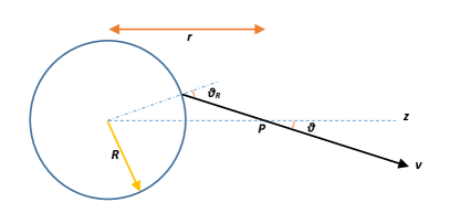
Figure 1: Geometry of the (neutrino) bulb model. Because of the spherical symmetry around the center of the supernova and the axial symmetry around the radial ($z$) direction, a neutrino beam is uniquely determined by its emission angle $\vartheta_{R}$ on the surface of the neutron star (of radius $R$). The polar angle $\vartheta(r)$ which the neutrino beam makes with the $z$ direction at point $P$ depends on the distance $r$ of $P$ from the center of the supernova. The azimuthal angle $\varphi$ around the $z$ axis (not shown) is also needed to describe the direction of the neutrino beam in the extended bulb model which does not have the axial symmetry around the $z$ axis.

In the bulb model it is assumed that both the neutrino emission and the supernova environment are stationary because the evolution timescale of the supernova is much longer than that of neutrino oscillations. It is further assumed that the supernova is spherically symmetric around its center so that only radius $r$ or the distance from the center of the supernova is needed to describe the spatial coordinate the neutrino. All the neutrinos are emitted from the surface of the spherical neutron star of radius $R$ and stream through the supernova envelope with the speed of light $c$ without hindering. The neutrino emission in the bulb model is assumed to be axially symmetric around the radial direction. Therefore, the propagation direction of a neutrino beam is uniquely determined by its emission angle $\vartheta_{R}=\vartheta(R)$ on the surface of the neutron star or, equivalent, by the polar angle $\vartheta(r)$ between the propagation direction of the neutrino and the radial direction (see Fig. 1).

The flavor quantum state of a neutrino or antineutrino (i.e. the antiparticle of the neutrino) in the bulb model is described by a multi-component complex wavefunction

$$\psi_{\nu_{\alpha}}(E,\bm{\hat{\mathbf{v}}};r)=\begin{pmatrix}a\\ b\end{pmatrix}\qquad\text{or}\qquad\psi_{\bar{\nu}_{\alpha}}(E,\bm{\hat{\mathbf{v}}};r)=\begin{pmatrix}\bar{a}\\ \bar{b}\end{pmatrix},$$ (1)

where $\alpha$ is the initial flavor of the neutrino at radius $R$, $E$ is the energy of the neutrino, and $\bm{\hat{\mathbf{v}}}$ is the unit vector along the propagation direction of the neutrino. As in Ref. [6] we assume a flavor mixing between two flavors $e$ and $x$ only, where $\nu_{x}$ is a linear combination of $\nu_{\mu}$ and $\nu_{\tau}$. Generalization to the three-flavor mixing can also be done [7, 8]. In Eq. (1) $a$ and $b$ are the amplitudes of the neutrino to be in the $e$ and $x$ flavors, respectively, and, therefore, $|a|^{2}$ and $|b|^{2}$ give the probabilities for the neutrino to be detected in the corresponding flavors.

The flavor content of the neutrino medium can solved from the Schrödinger equation

$$\mathrm{i}\cos\vartheta\,\partial_{r}\psi_{\nu_{\alpha}}(E,\bm{\hat{\mathbf{v}}};r) =\mathsf{H}\,\psi_{\nu_{\alpha}}(E,\bm{\hat{\mathbf{v}}};r)=[\mathsf{H}_{\text{vac}}(E)+\mathsf{H}_{\text{mat}}(r)+\mathsf{H}_{\nu\nu}(\bm{\hat{\mathbf{v}}};r)]\,\psi_{\nu_{\alpha}}(E,\bm{\hat{\mathbf{v}}};r),$$ (2a)

$$\mathrm{i}\cos\vartheta\,\partial_{r}\psi_{\bar{\nu}_{\alpha}}(E,\bm{\hat{\mathbf{v}}};r) =\bar{\mathsf{H}}\,\psi_{\bar{\nu}_{\alpha}}(E,\bm{\hat{\mathbf{v}}};r)=[\mathsf{H}_{\text{vac}}(E)-\mathsf{H}_{\text{mat}}(r)-\mathsf{H}_{\nu\nu}^{*}(\bm{\hat{\mathbf{v}}};r)]\,\psi_{\bar{\nu}_{\alpha}}(E,\bm{\hat{\mathbf{v}}};r),$$ (2b)

where $\partial_{r}$ is the partial differentiation with respect to $r$, $\mathsf{H}_{\text{vac}}$ is the standard vacuum Hamiltonian, and $\mathsf{H}_{\text{mat}}$ and $\mathsf{H}_{\nu\nu}$ are the matter and neutrino potentials, respectively. Here we have adopted the natural units with both the (reduced) Planck constant $\hbar$ and the speed of light $c$ equal to 1. In the two-flavor mixing scenario the vacuum Hamiltonian

$$\mathsf{H}_{\text{vac}}(E)=\frac{\Delta m^{2}}{4E}\,\begin{pmatrix}-\cos 2\theta_{\text{v}}&\sin 2\theta_{\text{v}}\\ \sin 2\theta_{\text{v}}&\cos 2\theta_{\text{v}}\end{pmatrix}$$ (3)

depends on the neutrino energy $E$ and two key parameters of neutrino mixing: the mass-squared difference $\Delta m^{2}$ and the vacuum mixing angle $\theta_{\text{v}}$ [2]. The matter potential is

$$\mathsf{H}_{\text{mat}}(r)=\sqrt{2}G_{\text{F}}n_{e}(r)\,\begin{pmatrix}1&0\\ 0&0\end{pmatrix},$$ (4)

where $G_{\text{F}}\approx 1.166\times 10^{-5}\,\text{GeV}^{-2}$ is the Fermi coupling constant for the weak interaction, and $n_{e}(r)$ is the electron number density at radius $r$. The difficulty of solving Eq. (2) stems from the neutrino potential

$$\mathsf{H}_{\nu\nu}(\bm{\hat{\mathbf{v}}};r)=\frac{\sqrt{2}G_{\text{F}}}{2\pi R^{2}}\sum_{\alpha^{\prime}}\int_{0}^{1}\mathrm{d}(\cos\vartheta^{\prime})\int_{0}^{\infty}\mathrm{d}E^{\prime}\,(1-\bm{\hat{\mathbf{v}}}\cdot\bm{\hat{\mathbf{v}}}^{\prime})\,\mathsf{F}_{\alpha^{\prime}}(E^{\prime};\bm{\hat{\mathbf{v}}}^{\prime};r),$$ (5)

which couples the flavor evolution of all the neutrinos and antineutrinos. In the above equation

$$1-\bm{\hat{\mathbf{v}}}\cdot\bm{\hat{\mathbf{v}}}^{\prime}=1-\cos\vartheta\cos\vartheta^{\prime},$$ (6)

and

$$\mathsf{F}_{\alpha}(E,\bm{\hat{\mathbf{v}}};r)=\frac{L_{\nu_{\alpha}}}{\langle E_{\nu_{\alpha}}\rangle}\,f_{\nu_{\alpha}}(E)\,[\psi_{\nu_{\alpha}}(E,\bm{\hat{\mathbf{v}}};r)\,\psi_{\nu_{\alpha}}^{\dagger}(E,\bm{\hat{\mathbf{v}}};r)]-\frac{L_{\bar{\nu}_{\alpha}}}{\langle E_{\bar{\nu}_{\alpha}}\rangle}\,f_{\bar{\nu}_{\alpha}}(E)\,[\psi_{\bar{\nu}_{\alpha}}(E,\bm{\hat{\mathbf{v}}};r)\,\psi_{\bar{\nu}_{\alpha}}^{\dagger}(E,\bm{\hat{\mathbf{v}}};r)]^{*},$$ (7)

where $L$, $\langle E\rangle$ and $f(E)$ are the energy luminosities, average energies and normalized energy distribution functions of the correspond neutrinos and antineutrinos on the surface of the neutron star.

It has been shown recently that the axial symmetry of the neutrino flavor wavefunction around the radial direction can be broken spontaneously by collective neutrino oscillations [9, 10]. In this case it seems natural to generalize the bulb model to the extended bulb model in which $\bm{\hat{\mathbf{v}}}$ is determined by both the azimuthal angle $\varphi$ around the radial direction and the polar angle $\vartheta$. Correspondingly, one should make the replacements

$$1-\bm{\hat{\mathbf{v}}}\cdot\bm{\hat{\mathbf{v}}}^{\prime} \longrightarrow 1-[\cos\vartheta\cos\vartheta^{\prime}+\sin\vartheta\sin\vartheta^{\prime}(\cos\varphi\cos\varphi^{\prime}+\sin\varphi\sin\varphi^{\prime})],$$ (8)

$$\int_{0}^{1}\mathrm{d}(\cos\vartheta^{\prime}) \longrightarrow\frac{1}{2\pi}\int_{0}^{2\pi}\mathrm{d}\varphi^{\prime}\int_{0}^{1}\mathrm{d}(\cos\vartheta^{\prime})$$ (9)

in Eq. (5). However, we note that the extended bulb model is not a self-consistent model because it is not possible to maintain the (spatial) spherical symmetry about the center of the neutron star without the (directional) axial symmetry around the radial direction. Nevertheless, because of the lack of a better model, we will use the extended bulb in our evaluation of the MIC architecture.

We note that the neutrino potential $\mathsf{H}_{\nu\nu}(\bm{\hat{\mathbf{v}}};r)$ in Eq. (5) is the same for all the neutrinos with the same propagation direction $\bm{\hat{\mathbf{v}}}$ and does not depend on the energy $E$ of the neutrino. Further, in the extended bulb model the same few weighted integrals are needed in computing $\mathsf{H}_{\nu\nu}(\bm{\hat{\mathbf{v}}};r)$ for all neutrino beams:

$$\Phi_{1}(r) =\sum_{\alpha}\int_{0}^{1}\mathrm{d}(\cos\vartheta)\int_{0}^{2\pi}\mathrm{d}\varphi\int_{0}^{\infty}\mathrm{d}E\,\mathsf{F}_{\alpha}(E,\bm{\hat{\mathbf{v}}};r),$$ (10a)

$$\Phi_{\mathrm{c}}(r) =\sum_{\alpha}\int_{0}^{1}\mathrm{d}(\cos\vartheta)\,\cos\vartheta\int_{0}^{2\pi}\mathrm{d}\varphi\int_{0}^{\infty}\mathrm{d}E\,\mathsf{F}_{\alpha}(E,\bm{\hat{\mathbf{v}}};r),$$ (10b)

$$\Phi_{\mathrm{sc}}(r) =\sum_{\alpha}\int_{0}^{1}\mathrm{d}(\cos\vartheta)\,\sin\vartheta\int_{0}^{2\pi}\mathrm{d}\varphi\,\cos\varphi\int_{0}^{\infty}\mathrm{d}E\,\mathsf{F}_{\alpha}(E,\bm{\hat{\mathbf{v}}};r),$$ (10c)

$$\Phi_{\mathrm{ss}}(r) =\sum_{\alpha}\int_{0}^{1}\mathrm{d}(\cos\vartheta)\,\sin\vartheta\int_{0}^{2\pi}\mathrm{d}\varphi\,\sin\varphi\int_{0}^{\infty}\mathrm{d}E\,\mathsf{F}_{\alpha}(E,\bm{\hat{\mathbf{v}}};r).$$ (10d)

This observation simplifies the numerical implementation greatly.

3 Numerical implementation

We developed a C++ code XFLAT largely based on the algorithm explained in Ref. [11]. Here we highlight the modifications and optimization for the MIC architecture [12].

3.1 Utilization of Xeon Phi

The first generation Xeon Phi KNC is in the form of coprocessor or accelerator packaged as a PCIe card. The second generation Xeon Phi is or will be in both forms of processor and coprocessor. Even though KNC works as an add-on accelerator, it supports the native mode in which it runs its own OS and can function as an independent MPI node. In implementing XFLAT we decided to take advantage of the similarities of the x86 and MIC architectures and created a single code base which can be compiled and run on both architectures. When MPI is enabled, a separate MPI task is run on each CPU and Xeon Phi accelerator which we now loosely refer to a “computing unit”. In each MPI task OpenMP threads employed to exploit the multi-processing power of each computing unit.

3.2 Discretization and data structure

In XFLAT a group or “beam” of neutrinos with the same propagation direction $\bm{\hat{\mathbf{v}}}$ and initial particle identity (i.e. $\nu_{e}$, $\nu_{x}$, $\bar{\nu}_{e}$ or $\bar{\nu}_{x}$) is described by an NBeam object. For the two-flavor mixing scenario an NBeam object consists of 4 floating point arrays, ar[E_CNT], ai[E_CNT], br[E_CNT] and bi[E_CNT], which are the real and imaginary components of the neutrino wavefunctions of the neutrinos in the beam [see Eq. (1)]. For simplicity we have discretized the continuous energy distributions or energy spectra of the neutrino into energy bins of equal energy intervals, and E_CNT is the total number of energy bins.

The flavor quantum state $\{\psi_{\nu_{\alpha}}(E,\bm{\hat{\mathbf{v}}};r),\psi_{\bar{\nu}_{\alpha}}(E,\bm{\hat{\mathbf{v}}};r)\}$ of the neutrino medium at radius $r$ is represented by a three dimensional object array NBeam[THETA_CNT][PHI_CNT][PARTICLE_CNT], where THETA_CNT, PHI_CNT and PARTICLE_CNT are the numbers of polar angle ($\vartheta$) bins, azimuthal angle ($\varphi$) bins and initial particle identities, respectively. The continuous neutrino flux distribution in the polar angle $\vartheta$ and azimuthal angle $\varphi$ is discretized as equal-sized bins of $u=\sin^{2}\vartheta_{R}$ and $\varphi$ within ranges $u\in[0,1]$ and $\varphi\in[0,2\pi)$, respectively. We chose this discretization scheme because, if the overall neutrino flux is uniform in terms of the differential solid angle $\mathrm{d}(\cos\vartheta)\,\mathrm{d}\varphi$, it will also be (almost) uniform in terms of $\mathrm{d}u\,\mathrm{d}\varphi$ at $r\gg R$.

In XFLAT the first dimension (in polar angle $\vartheta$) of the NBeam array is actually divided into several sections each of which is located in the memory of a separate compute device (i.e., a CPU or Xeon Phi accelerator). The number of polar angle bins, THETA_CNT_LOCAL, on each device depends on its relative computing capability.

3.3 SoA data structure and SIMD parallelization

The NBeam object in XFLATuses a Structure-of-Arrays (SoA) arrangement. In contrast Ref. [11] defines the NBeam object as an Array of Structures (AoS). In the AoS arrangement an NBeam object consists of an array PSI[E_CNT]. Each element of this array is an object PSI which represents the wavefunction of a single neutrino and consists of 4 floating point numbers, ar, ai, br and bi.

The Intel Xeon Phi accelerator is capable of performing same instructions on multiple data (SIMD) simultaneously. The SoA implementation of the NBeamobject in XFLAT facilitates the SIMD parallelization provided by the MIC architecture.

3.4 Numerical algorithm and parallelization

XFLAT solves Eq. (2) as an initial condition problem with initial conditions

$$\psi_{\nu_{e}}(E,\bm{\hat{\mathbf{v}}};r=R) =\psi_{\bar{\nu}_{e}}(E,\bm{\hat{\mathbf{v}}};r=R)=\begin{pmatrix}1\\ 0\end{pmatrix}, \psi_{\nu_{x}}(E,\bm{\hat{\mathbf{v}}};r=R) =\psi_{\bar{\nu}_{x}}(E,\bm{\hat{\mathbf{v}}};r=R)=\begin{pmatrix}0\\ 1\end{pmatrix}.$$ (11)

The basic algorithm that evolves the neutrino wave function over a small radial step $\delta r$ is [6]

$$\psi_{\nu}(E,\bm{\hat{\mathbf{v}}};r+\delta r) =\exp(-\mathrm{i}\mathsf{H}\,\delta l)\,\psi_{\nu}(E,\bm{\hat{\mathbf{v}}};r)$$ (12a)

$$=\frac{1}{\lambda}\begin{pmatrix}\lambda\cos(\lambda\delta l)-\mathrm{i}h_{11}\sin(\lambda\delta l)&-\mathrm{i}h_{12}\sin(\lambda\delta l)\\ -\mathrm{i}h_{12}^{*}\sin(\lambda\delta l)&\lambda\cos(\lambda\delta l)+\mathrm{i}h_{11}\sin(\lambda\delta l)\end{pmatrix}\psi_{\nu}(E,\bm{\hat{\mathbf{v}}};r),$$ (12b)

where $\delta l=\delta r/\cos\vartheta$, $h_{11}$ and $h_{12}$ are the diagonal and off-diagonal elements of the total Hamiltonian $\mathsf{H}$, respectively, and $\lambda=\sqrt{h_{11}^{2}+|h_{12}|^{2}}$. On top of this algorithm XFLAT uses a modified mid-point integration solver with adaptive step-size control [11].

XFLAT implements a parallel version of the above algorithm which utilizes all three levels of parallelism provided by the MIC architecture, i.e., SIMD within an thread, OpenMP threads within a compute device and MPI among different compute devices (see Fig. 2).

In computing the neutrino potential $\mathsf{H}_{\nu\nu}$ [see Eqs. (5) and (9)] the innermost integral over the neutrino energy in Eq. (10) is performed by a for loop with the OpenMP SIMD directive.

is computed by the summation or integration of the contributions from all neutrino beams [see Eqs. (5) and (9)]. This summation is carried out by using all three levels of parallelism provided by the MIC architecture. At the top level the whole range of the polar angle $\vartheta$ is broken down into several sections, and the At the lowest level the summation over neutrino energy bins is performed inside each OpenMP thread by using the OpenMP SIMD directive. This corresponds to the innermost integral over the neutrino energy in (10). in Eqs. (5), (10) and (12).

However, this Array-of-Structure (AoS) design does not work well with the SIMD units on MIC or the modern CPUs (see, e.g., [13]). Instead, we adopt a Structure-of-Array (SoA) design and define four arrays in each NBeam object: ar$[E]$, ai$[E]$, br$[E]$ and bi$[E]$, which represent the real and imaginary parts of the upper and lower components of the wavefunction in Eq. (1). The omp simd pragma is then used to instruct the compiler to vectorize the code so that the procedure in Eq. (12) can be applied to multiple neutrino wavefunctions (8 for KNC and 4 for the E5-2869 Xeon CPU) simultaneously through the SIMD units (see Fig. LABEL:fig:simd).

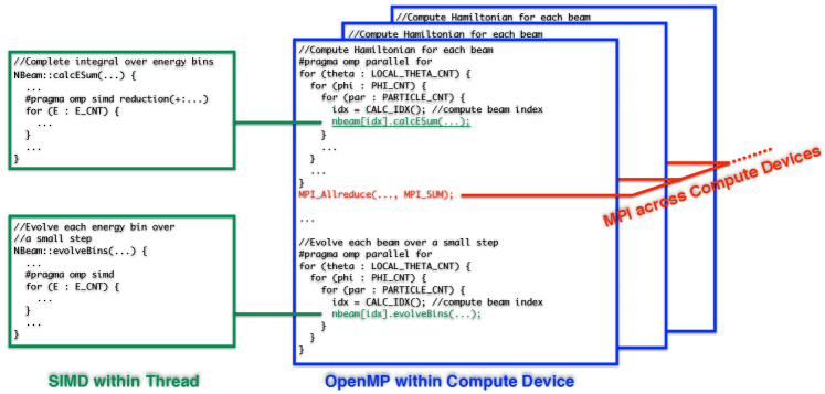
Figure 2: The evolveBins method of the NBeam object which evolves the wavefunctions in the neutrino beam for a small radial step by using the procedure described in Eq. (12). The omp simd pragma instructs the compiler to generate a vectorized code which utilizes the SIMD units on MIC.

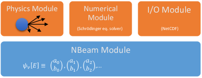
Figure 3: The dual-layer design of XFLAT. The NBeam module on the lower-level implements an array of the wavefunctions of the neutrinos with the same initial flavor and propagation direction. It adopts the SoA (Structure of Array) data structure to utilize efficiently the SIMD units on MIC. The upper-level modules implement the physics and geometry of the supernova model, the numerical algorithm for solving the Schrödinger equation and the data I/O, respectively. They adopt the AoS (Array of Structure) data structure and are designed to be flexible.

XFLAT adopts a dual-layer modular design (see Fig. 3). The lower-level module defines the NBeam object. On top this module are three modules which operate closely with each other and carry out different tasks:

• The Physics Module describes the physics and geometry of the supernova model and provides the methods for computing the matter potential $\mathsf{H}_{\text{mat}}$ and the neutrino potential $\mathsf{H}_{\nu\nu}$.

• The Numerical Module implements a modified midpoint method described in Ref. [11] to solve the differential equation (2).

• The I/O Module performs data input and output by using the netCDF library [14].

Unlike the NBeam Module which is optimized for the SIMD units by with the SoA data structure, the three upper-level modules use the AoS design to take advantage of the Object-Oriented Programming (OOP) paradigm of C++. For example, the Physics Module defines the NBGroup object which include all the neutrino beams and is essentially an array of NBeam objects.

As in Ref. [11] each of the four modules of XFLAT is carefully crafted to be independent of the internal details of other modules. For example, we have implemented the Physics Modules for both the bulb model and the extended bulb model. One can use XFLAT to carry out the calculations for either model by choosing the appropriate Physics Module without modifying the rest of the code.

XFLAT uses all the three levels of parallelism provided by MIC. At the top level the MPI is used to divide the full NBeam array of the NBGroup object into subarrays and assign them to different MPI processes or ranks on the available compute devices (CPUs and/or Xeon Phis). XFLAT utilizes the native mode of the Xeon Phi coprocessor such that each Xeon Phi runs an independent MPI process and is treated as an “ordinary” CPU compute node except with more cores and wider SIMD units. At the middle level the operations on the subarray of NBeam objects is carried out in parallel on the many cores (and hyperthreads) on the CPU or Xeon Phi via OpenMP. At the bottom level the operations on the individual neutrino wavefunctions inside each NBeam object are performed in parallel on the SIMD units using the omp simd pragma. For example, the integration over energy $E$ in Eq. (10) is carried out within each thread using the SIMD units with the omp simd reduction pragma, and the integration over angles $\vartheta$ and $\varphi$ is performed first inside each MPI process using OpenMP with the omp parallel for reduction pragma and then across the MPI processes with the MPI_Allreduce function call.

We validate XFLAT by comparing its results for the bulb model and the extended bulb model for the scenarios where the axial symmetry around the radial direction is not broken. We also compare its results for the bulb model with those in the literature [12]. In Fig. 4 we show the results of the bulb model computed using XFLAT using the same neutrino mixing parameters and the so-called “single-split spectra” in Ref. [15]. The results produced by XFLAT agree very well with those in Ref. [15] which are based on a numerical code developed independently at the Northwestern University [16].

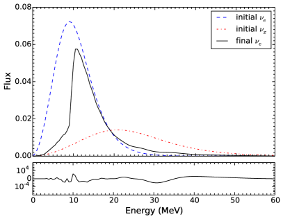
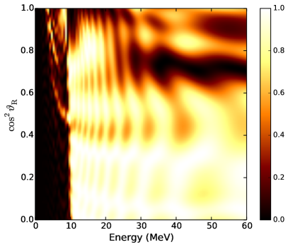
Figure 4: Top left: The initial number fluxes of the neutrino in the electron ($\nu_{e}$, dashed curve) and the other flavor ($\nu_{x}$, dotted curve) in some arbitrary units on the surface of the neutron star and the $\nu_{e}$ flux at $r=250\,\text{km}$ as functions of neutrino energy $E$ in the bulb model as computed by XFLAT. Bottom left: The absolute difference between the $\nu_{e}$ fluxes at $r=250\,\text{km}$ between the XFLAT result and that of the “SS spectra” case in Ref. [15]. Right: Neutrino survival probability $P_{ee}=|a_{e}|^{2}$ (represented by the color scale) at $r=250\,\text{km}$ in the bulb model computed by XFLAT as a function of the neutrino energy $E$ and emission angle $\vartheta_{R}$ on the surface of the neutron star.

4 Performance analysis

We analyze the performance of XFLAT on the KNL nodes of the Cori supercomputer at NERSC (see Table LABEL:tab:nersc for its hardware specifications). Double precision was used exclusively in all floating point calculations. For all the benchmarks reported here XFLAT was compiled with the Intel C++ compiler (v18.0.3) with flags -O3 -openmp -xMIC-AVX512. One XFLAT process was run on each KNL. Each process was run with 272 OpenMP threads to fully utilize its hyperthreading capability. For MPI-enabled benchmarks the Intel MPI library 2018 was used. Unless stated otherwise, all the calculations are for a “standard problem”

Table 1: The hardware specifications of the compute nodes of the Cori supercomputer [17].

Component	Specifications
CPU	$1\times$ Knights Landing 7250 (68 cores, 272 threads) @1.4GHz
Memory	96GB ($6\times$ 16GB) DDR4 @2400MHz
MCDRAM	16GB on-package, high-bandwidth memory

4.1 Single-node performance

We first benchmarked the raw performance of KNL on a single compute node for double precision multiply/add floating point operations (left panel in Fig. 5). Since, XFLAT extensively employs transcendental functions, we also benchmarked the performance of KNL for sin/cos, and exponent, respectively (right panel in Fig. 5). In the innermost loop of the benchmark kernels simple floating point operations are performed on an array or vector of double-precision (DP) floating-point numbers. The widths of the vectors are chosen to be a multiple of that of the SIMD registers of the computing component (512 bits or 8 DP for the Xeon Phi). We changed the length of the most inner loop from 8 (2³) to 1024 (2¹⁰). The same vector operations are repeated 10 million times in the middle loop to maintain data locality in the processor’s cache. In the outermost loop all of the hardware threads are utilized to achieve the best performance.

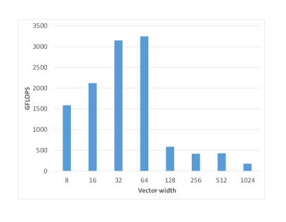
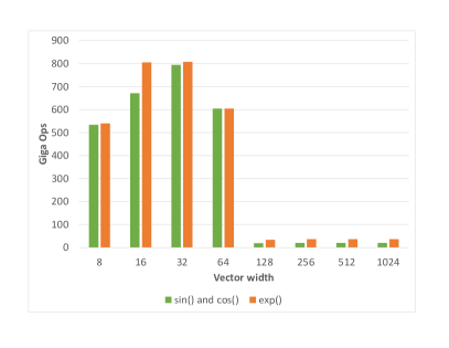
Figure 5: The performance of KNL on a single compute node of Cori. Left: The floating point operations for computing a multiply and an add operations as functions of the length of the innermost vectorized loop. Right: The performance of the chip for a sine and cosine operations per iteration, and one exponent operation per each loop iteration.

As it is noticeable, the performance improved by increasing the vector width in the beginning, however, it dropped sharply by going beyond 64 in both plots. Part of the reason might be due to the internal caching mechanism that works well up to the size of 512 bytes. Similar results has been reported on KNC[DBLP:journals/corr/NoormofidiAD15].

Next, we benchmarked XFLAT on a single KNL using two different memory mode. The MCDRAM on KNL can work on three different configurations: Cache mode, Flat mode, and Hybrid mode. In Cache mode MCDRAM acts as a cache layer between the processor’s internal last level cache and DRAM. In Flat mode the MCDRAM acts as a software regular memory residing in the same address space as DRAM. In the Hybrid mode MCDRAM is the combination of the former two modes (part cache and part memory).

As shown in right panel of Fig. 6 the run times of these tests scale approximately linearly with problem size. Also the performance of Flat mode is slightly better, however, it requires that the application explicitly allocates memory on the second NUMA domain, since in the Flat mode the MCDRAM memory is shown as the second NUMA domain. In addition, the last two data points show that the memory footprint of XFLAT was too high (>16 GB) to fit into MCDRAM in the Flat mode.

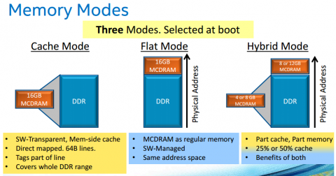
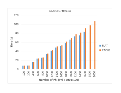
Figure 6: Left: The KNL memory modes (image courtesy of NERSC). Right: The timing of XFLAT (calculating 100 radial steps) for the Flat and the Cache memory mode.

4.2 Multi-node performance

We benchmarked XFLAT on multiple compute nodes. For the multi-node benchmarks we fixed the number of azimuth bins to 10 and number of energy bins to 100, then increased the number of polar angle bins in the “standard problem” from $10,000$ to $30,000$. The number of nodes were also varied from 2 to more than 32 nodes. In each of the tests we ran XFLAT without any disk I/O for approximately 100 seconds and computed the number of calculated steps per second. All the benchmarks were performed with MCDRAM configured in Cache mode. In the left panel of Fig. 7 the performance of XFLAT is shown as a function of number of compute nodes. The benchmarks were repeated for $10,000$, $20,000$, and $30,000$ polar angles. These benchmarks show that the performance of XFLAT scales well and if there are enough jobs (i.e. polar angle bins), the scalibility is almost linear. The reason for the step pattern in the plot is due to having a load imbalance among threads/cores on KNL, as discussed in [DBLP:journals/corr/NoormofidiAD15]. So the reason for the poor scaling behavior is because the 272 hardware threads of the Xeon Phi cannot not be fully utilized for the studied problem size when many compute nodes are used. For example, in the test with $10,000$ polar angles on 18 compute nodes each Xeon Phi process received almost $555(\approx 10,000/18)$ polar angle bins, which is just a few more than twice the 272 threads available on the Xeon Phi. As a result, the OpenMP parallel for loop iterated three times in each step with most of the threads idle in the last iteration. When 20 compute nodes were used, however, each Xeon Phi process received 500 polar angle bins, and the computation for these angle bins was completed in two iterations by employing most of the threads. For low amount of load the performance of XFLAT does not increase much when more compute nodes are used because there is not enough load on each Xeon Phi (and consequently on each thread).

In the right panel of Fig. 7 the performance of XFLAT is shown as a function of load (i.e. polar angle bins) on various multi-node configurations. As one may notice again, distributing the load on many number of nodes will result in load imbalance on KNL’s threads.

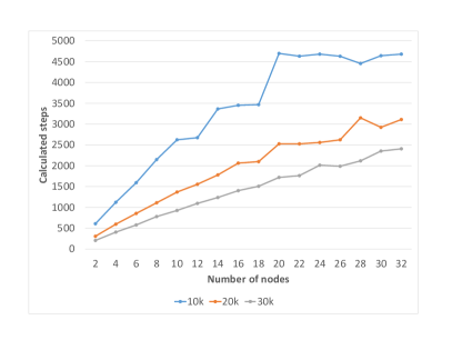
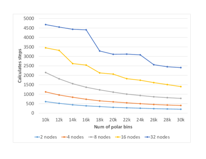
Figure 7: Left: The number of calculated radial steps on computing 10k, 20k, and 30k angle bins in about 100 seconds. Right: The XFLAT performance on 2, 4, 8, 16, and 32 nodes with various number of polar bins (number of calculated radial steps per 100s).

Fig. 8 shows the scalibility and saturation point of XFLAT. In the left panel, one can see the scalibility of the application for three different polar angle loads on up to 256 compute nodes. It is noticeable that by going to more compute nodes, the performance peaks and then drops, since there is not enough load (low number of polar bins). Adding each compute node result in increase the communications overhead to the system, however, individual threads do not have enough compute load to process. In the right panel, the number of nodes is fixed to between 48 and 256, but the load (number of polar bins) varies from 10k to 30k. For each node configuration, the performance is steady until reaching a critical point, then drops to the next level. This behavior is also due to the load imbalance on each KNL’s threads which is caused by the change in the number of polar bins. The performance drop points for the run with 128 and 256 nodes only happen by going beyond 30k polar angle bins (not shown here).

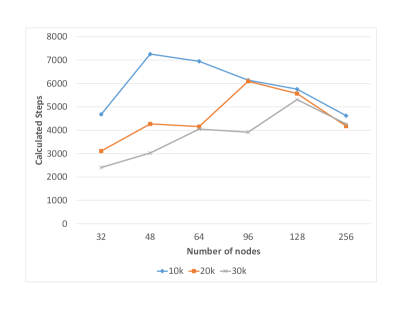
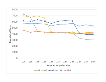
Figure 8: Left: Scalibility of XFLAT on various number of nodes (2 to 256) for three different loads: 10k, 20k, and 30k polar bins. Right: XFLAT’s performance when the number of nodes is fixed at 48, 64, 96, 128, or 256.

Fig. 9 depicts the full range of our benchmarks starting from $10,000$ polar bins to $30,000$ with $2,000$ incremental steps. It can be concluded that for a low amount of load, increasing the number of nodes does not result in performance improvement, since each hardware thread may not receive enough bins to keep the hardware fully loaded. For example, for the run with 10k polar bins, by going beyond 20 nodes the performance does not improve due to the same reason. On the contrary, the benchmark with 30k polar bins scale well even beyond 30 nodes. As a result, it is very important to choose the right number of compute node so that the load can distribute on all hardware thread evenly.

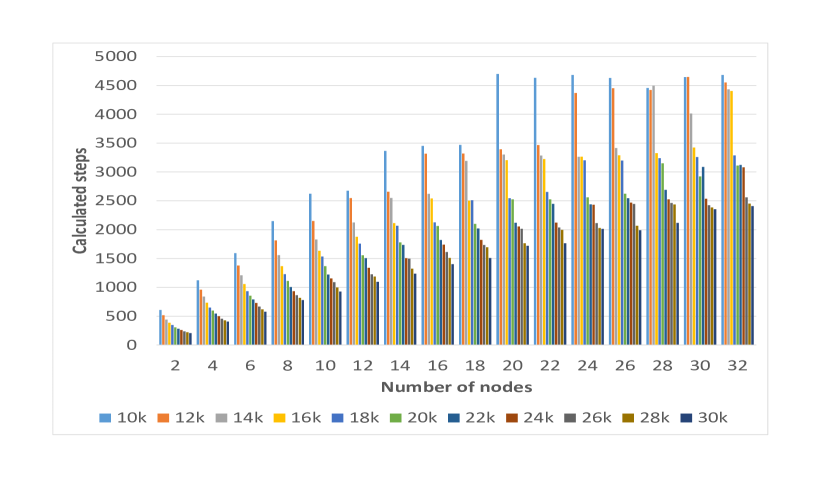
Figure 9: The overall performance of XFLAT over various number of nodes and number of polar bins (calculated steps for 100s).

5 Discussion and summary

In this work we explore the Intel MIC architecture by developing and benchmarking an astrophysical simulation code, XFLAT, which compute neutrino oscillations in supernovae. Our study is based on the extended (supernova neutrino) bulb model and the algorithm outlined in Ref. [11]. To fully utilize the SIMD units on the MIC architecture we have changed the low-level module, i.e. the NBeam module describing the neutrino beam, from the AoS layout to the SoA layout. This approach boosts the performance on both the MIC and CPU alike because modern CPUs also have SIMD units albeit with smaller widths than those on the MIC. We have applied three levels of parallelization in XFLAT: MPI for the inter-CPU/MIC parallelization, OpenMP for intra-CPU/MIC parallelization, and SIMD for the most fine-grained parallelization within each core.

We benchmarked XFLAT on the Stampede supercomputer which is equipped with the first-generation Xeon Phi or KNC. Our tests show that XFLAT achieves a speedup of $2.5$–$2.9$ on a single Xeon Phi relative to a single 8-core E5 Xeon CPU, although the Xeon Phi on the Stampede has a peak performance approximate 6 times that of the CPU. We note that, however, the performance of the floating point operations on the Xeon Phi depends on both the size of the omp for simd loop and the nature of the operations. For example, the performance of the double-precision exp function on the KNC is approximately 4 times of that on the CPU [19]. The Xeon CPU has large caches per core than the KNC which may have also play a role in our performance tests.

In Fig. 10 we compare the speedup of XFLAT on Stampede due the Xeon Phis with those in applications for the critical Ising model (CIM [20]), quantum chemistry (QC1 [21] and QC2 [22]), thermo-hydrodynamics (TH [23]), experimental high-energy physics (HEP [24]), molecular visualization (MV [25]), molecular dynamics (MD [26]), dynamics of astrophysical objects (DAO [27]), protein database search (PDS [28]), synthetic aperture radar (SAR [29]) and microscopic image analysis (MIA [30]). In presenting this comparison we plot the speedups because of the Xeon Phi versus the peak performance ratio between the Xeon Phi and CPU or

$$\xi=\frac{P_{\text{MIC}}}{P_{\text{CPU}}},$$ (13)

where

$$P_{\text{device}}=(\text{width of the SIMD unit per core})\times(\text{number of cores per device})\times(\text{device clock rate}).$$ (14)

It seems that most of the applications achieve a speed up of $\xi/2$ or less.

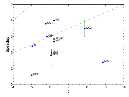
Figure 10: The speedups because of the Xeon Phi coprocessor in various applications which were run on computer with various MIC-CPU peak performance ratios ($\xi$). The error bars represented the reported the ranges of the speedups. The two dotted lines correspond to the scenarios with the speedup equal $\xi$ and $\xi/2$, respectively.

We have adopted the native mode of the Xeon Phi hoping that the same code can run on both the CPU and the MIC. However, because the I/O performance of the KNC is very poor compared to the CPU, we have to implement different I/O modules for the MIC and the CPU so that the CPU writes the data on behalf the Xeon Phi to the disk.

In multi-node tests we found that it was more difficult to fully utilize the computing capability of the Xeon Phi than that of the CPU because the Xeon Phi has many more but less powerful cores than the CPU. Further, it can also be a challenge to maintain the load balance in a heterogeneous environment where both the CPU and Xeon Phi are employed. There can be a significant drop in the performance of the Xeon Phi when the number of jobs on the device is slightly more than a multiple of the number of its hardware threads ($\sim 240$).

It has recently been shown that the spherical symmetry and stationary assumption employed in the extended bulb model could be broken spontaneously by neutrino oscillations [31, 32]. As a result, simulations in full 7-dimensional supernova models (with 1 temporal, 3 spatial and 3 momentum dimensions) must be performed in order to study the real impacts of neutrino oscillations on supernova physics. This paradigm shift implies a dramatic increase of several orders of magnitude in computational intensity which can be a good fit for the next-generation MIC supercomputers.

References

References

- [1] S. Woosley, T. Janka, The physics of core-collapse supernovae, Nat. Phys. 1 (2005) 147.
- [2] K. A. Olive, et al., Review of particle physics, Chin. Phys. C38 (2014) 090001.
- [3] A. Mirizzi, I. Tamborra, H.-T. Janka, N. Saviano, K. Scholberg, R. Bollig, L. Hudepohl, S. Chakraborty, Supernova Neutrinos: Production, Oscillations and DetectionarXiv:1508.00785.
- [4] H. Duan, G. M. Fuller, Y.-Z. Qian, Collective neutrino oscillations, Ann. Rev. Nucl. Part. Sci. 60 (2010) 569. arXiv:1001.2799.
- [5] A. Vlasenko, G. M. Fuller, V. Cirigliano, Neutrino Quantum Kinetics, Phys. Rev. D89 (10) (2014) 105004. arXiv:1309.2628, doi:10.1103/PhysRevD.89.105004.
- [6] H. Duan, G. M. Fuller, J. Carlson, Y.-Z. Qian, Simulation of coherent non-linear neutrino flavor transformation in the supernova environment: Correlated neutrino trajectories, Phys. Rev. D74 (2006) 105014. arXiv:astro-ph/0606616.
- [7] H. Duan, G. M. Fuller, J. Carlson, Y.-Z. Qian, Flavor Evolution of the Neutronization Neutrino Burst from an O-Ne-Mg Core-Collapse Supernova, Phys. Rev. Lett. 100 (2008) 021101. arXiv:0710.1271, doi:10.1103/PhysRevLett.100.021101.
- [8] J. F. Cherry, G. M. Fuller, J. Carlson, H. Duan, Y.-Z. Qian, Multi-Angle Simulation of Flavor Evolution in the Neutrino Neutronization Burst From an O-Ne-Mg Core-Collapse Supernova, Phys. Rev. D82 (2010) 085025. arXiv:1006.2175, doi:10.1103/PhysRevD.82.085025.
- [9] G. Raffelt, S. Sarikas, D. d. S. Seixas, Axial symmetry breaking in self-induced flavor conversion of supernova neutrino fluxes, Phys. Rev. Lett. 111 (2013) 091101. arXiv:1305.7140, doi:10.1103/PhysRevLett.111.091101.
- [10] A. Mirizzi, Multi-azimuthal-angle effects in self-induced supernova neutrino flavor conversions without axial symmetry, Phys. Rev. D 88 (7) (2013) 073004. arXiv:1308.1402.
- [11] H. Duan, G. M. Fuller, J. Carlson, Simulating nonlinear neutrino flavor evolution, Comput. Sci. Disc. 1 (2008) 015007. arXiv:0803.3650, doi:10.1088/1749-4699/1/1/015007.
- [12] V. Noormofidi, Simulating nonlinear neutrino oscillations on next-generation many-core architectures, Ph.D. thesis, University of New Mexico (2015).
- [13] J. Jeffers, J. Reinders, Intel Xeon Phi Coprocessor High-Performance Programming, Morgan Kaufmann, San Diego, CA, 2013.
-
[14]
Unidata, netCDF version 4.4.0
[software] (2016).
URL http://doi.org/10.5065/D6H70CW6 - [15] H. Duan, S. Shalgar, Multipole expansion method for supernova neutrino oscillations, JCAP 1410 (10) (2014) 084. arXiv:1407.7861, doi:10.1088/1475-7516/2014/10/084.
- [16] S. Shalgar, Transition magnetic moment and collective neutrino oscillations, Ph.D. thesis, Northwestern University (2013).
-
[17]
Cori
Xeon Phi nodes (2019 (accessed January 10, 2019)).
URL http://www.nersc.gov/users/computational-systems/cori/configuration/cori-intel-xeon-phi-nodes/ -
[18]
R. Rajachandrasekar, S. Potluri, A. Venkatesh, K. Hamidouche, M. Wasi-ur
Rahman, D. K. D. Panda,
Mic-check: A distributed
check pointing framework for the intel many integrated cores architecture,
in: Proceedings of the 23rd International Symposium on High-performance
Parallel and Distributed Computing, HPDC ’14, ACM, New York, NY, USA, 2014,
pp. 121–124.
doi:10.1145/2600212.2600713.
URL http://doi.acm.org/10.1145/2600212.2600713 - [19] V. Noormofidi, S. R. Atlas, H. Duan, Performance Analysis of an Astrophysical Simulation Code on the Intel Xeon Phi ArchitecturearXiv:1510.02163.
-
[20]
F. Wende, T. Steinke,
Swendsen-Wang
Multi-cluster Algorithm for the 2D/3D Ising Model on Xeon Phi and GPU, in:
Proceedings of the International Conference on High Performance Computing,
Networking, Storage and Analysis, SC ’13, ACM, New York, NY, USA, 2013, pp.
83:1–83:12.
doi:10.1145/2503210.2503254.
URL http://doi.acm.org/10.1145/2503210.2503254 -
[21]
E. Aprà, M. Klemm, K. Kowalski,
Efficient implementation of
many-body quantum chemical methods on the intel® xeon phi™
coprocessor, in: Proceedings of the International Conference for High
Performance Computing, Networking, Storage and Analysis, SC ’14, IEEE Press,
Piscataway, NJ, USA, 2014, pp. 674–684.
doi:10.1109/SC.2014.60.
URL http://dx.doi.org/10.1109/SC.2014.60 - [22] S. S. Leang, A. P. Rendell, M. S. Gordon, Quantum chemical calculations using accelerators: Migrating matrix operations to the nvidia kepler gpu and the intel xeon phi, Journal of Chemical Theory and Computation 10 (3) (2014) 908–912.
-
[23]
G. Crimi, F. Mantovani, M. Pivanti, S. Schifano, R. Tripiccione”,
Early
Experience on Porting and Running a Lattice Boltzmann Code on the Xeon-phi
Co-Processor, Procedia Computer Science 18 (0) (2013) 551 – 560, 2013
International Conference on Computational Science.
doi:http://dx.doi.org/10.1016/j.procs.2013.05.219.
URL http://www.sciencedirect.com/science/article/pii/S1877050913003621 -
[24]
V. Halyo, P. LeGresley, P. Lujan, V. Karpusenko, A. Vladimirov,
First evaluation of
the cpu, gpgpu and mic architectures for real time particle tracking based on
hough transform at the lhc, Journal of Instrumentation 9 (04) (2014) P04005.
URL http://stacks.iop.org/1748-0221/9/i=04/a=P04005 -
[25]
A. Knoll, I. Wald, P. A. Navrátil, M. E. Papka, K. P. Gaither,
Ray tracing and volume
rendering large molecular data on multi-core and many-core architectures,
in: Proceedings of the 8th International Workshop on Ultrascale
Visualization, UltraVis ’13, ACM, New York, NY, USA, 2013, pp. 5:1–5:8.
doi:10.1145/2535571.2535594.
URL http://doi.acm.org/10.1145/2535571.2535594 - [26] S. J. Pennycook, C. J. Hughes, M. Smelyanskiy, S. A. Jarvis, Exploring SIMD for Molecular Dynamics, Using Intel® Xeon® Processors and Intel® Xeon Phi Coprocessors, in: Parallel & Distributed Processing (IPDPS), 2013 IEEE 27th International Symposium on, IEEE, 2013, pp. 1085–1097.
-
[27]
I. Kulikov, I. Chernykh, A. Snytnikov, B. Glinskiy, A. Tutukov,
”astrophi:
A code for complex simulation of the dynamics of astrophysical objects using
hybrid supercomputers”, Computer Physics Communications 186 (2015) 71 – 80.
doi:http://dx.doi.org/10.1016/j.cpc.2014.09.004.
URL http://www.sciencedirect.com/science/article/pii/S0010465514003099 - [28] Y. Liu, B. Schmidt, SWAPHI: Smith-waterman protein database search on Xeon Phi coprocessors, in: Application-specific Systems, Architectures and Processors (ASAP), 2014 IEEE 25th International Conference on, IEEE, 2014, pp. 184–185.
- [29] J. Park, P. T. P. Tang, M. Smelyanskiy, D. Kim, T. Benson, Efficient backprojection-based synthetic aperture radar computation with many-core processors, Scientific Programming 21 (3-4) (2013) 165–179.
- [30] G. Teodoro, T. Kurc, J. Kong, L. Cooper, J. Saltz, Comparative Performance Analysis of Intel (R) Xeon Phi (TM), GPU, and CPU: A Case Study from Microscopy Image Analysis, in: Parallel and Distributed Processing Symposium, 2014 IEEE 28th International, IEEE, 2014, pp. 1063–1072.
- [31] H. Duan, S. Shalgar, Flavor instabilities in the neutrino line model, Phys. Lett. B747 (2015) 139–143. arXiv:1412.7097, doi:10.1016/j.physletb.2015.05.057.
- [32] S. Abbar, H. Duan, Neutrino flavor instabilities in a time-dependent supernova model, Phys. Lett. B751 (2015) 43–47. arXiv:1509.01538, doi:10.1016/j.physletb.2015.10.019.