Glauber dynamics on the Erdős-Rényi random graph

Abstract.

We investigate the effect of disorder on the Curie-Weiss model with Glauber dynamics. In particular, we study metastability for spin-flip dynamics on the Erdős-Rényi random graph $\mathrm{ER}_{n}(p)$ with $n$ vertices and with edge retention probability $p\in(0,1)$. Each vertex carries an Ising spin that can take the values $-1$ or $+1$. Single spins interact with an external magnetic field $h\in(0,\infty)$, while pairs of spins at vertices connected by an edge interact with each other with ferromagnetic interaction strength $1/n$. Spins flip according to a Metropolis dynamics at inverse temperature $\beta$. The standard Curie-Weiss model corresponds to the case $p=1$, because $\mathrm{ER}_{n}(1)=K_{n}$ is the complete graph on $n$ vertices. For $\beta>\beta_{c}$ and $h\in(0,p\chi(\beta p))$ the system exhibits metastable behaviour in the limit as $n\to\infty$, where $\beta_{c}=1/p$ is the critical inverse temperature and $\chi$ is a certain threshold function satisfying $\lim_{\lambda\to\infty}\chi(\lambda)=1$ and $\lim_{\lambda\downarrow 1}\chi(\lambda)=0$. We compute the average crossover time from the metastable set (with magnetization corresponding to the ‘minus-phase’) to the stable set (with magnetization corresponding to the ‘plus-phase’). We show that the average crossover time grows exponentially fast with $n$, with an exponent that is the same as for the Curie-Weiss model with external magnetic field $h$ and with ferromagnetic interaction strength $p/n$. We show that the correction term to the exponential asymptotics is a multiplicative error term that is at most polynomial in $n$. For the complete graph $K_{n}$ the correction term is known to be a multiplicative constant. Thus, apparently, $\mathrm{ER}_{n}(p)$ is so homogeneous for large $n$ that the effect of the fluctuations in the disorder is small, in the sense that the metastable behaviour is controlled by the average of the disorder. Our model is the first example of a metastable dynamics on a random graph where the correction term is estimated to high precision.

1. Introduction and main results

In Section 1.1 we provide some background on metastability. In Section 1.2 we define our model: spin-flip dynamics on the Erdős-Rényi random graph $\mathrm{ER}_{n}(p)$. In Section 1.3 we identify the metastable pair for the dynamics, corresponding to the ‘minus-phase’ and the ‘plus-phase’, respectively. In Section 1.4 we recall the definition of spin-flip dynamics on the complete graph $K_{n}$, which serves as a comparison object, and recall what is known about the average metastable crossover time for spin-flip dynamics on $K_{n}$ (Theorem 1.3 below). In Section 1.5 we transfer the sharp asymptotics for $K_{n}$ to a somewhat rougher asymptotics for $\mathrm{ER}_{n}(p)$ (Theorem 1.4 below). In Section 1.6 we close by placing our results in the proper context and giving an outline of the rest of the paper.

1.1. Background

Interacting particle systems, evolving according to a Metropolis dynamics associated with an energy functional called the Hamiltonian, may end up being trapped for a long time near a state that is a local minimum but not a global minimum. The deepest local minima are called metastable states, the global minimum is called the stable state. The transition from a metastable state to the stable state marks the relaxation of the system to equilibrium. To describe this relaxation, it is of interest to compute the crossover time and to identify the set of critical configurations the system has to visit in order to achieve the transition. The critical configurations represent the saddle points in the energy landscape: the set of mini-max configurations that must be hit by any path that achieves the crossover.

Metastability for interacting particle systems on lattices has been studied intensively in the past three decades. Various different approaches have been proposed, which are summarised in the monographs by Olivieri and Vares [13], Bovier and den Hollander [4]. Recently, there has been interest in metastability for interacting particle systems on random graphs, which is much more challenging because the crossover time typically depends in a delicate manner on the realisation of the graph.

In the present paper we are interested in metastability for spin-flip dynamics on the Erdős-Rényi random graph. Our main result is an estimate of the average crossover time from the ‘minus-phase’ to the ‘plus-phase’ when the spins feel an external magnetic field at the vertices in the graph as well as a ferromagnetic interaction along the edges in the graph. Our paper is part of a larger enterprise in which the goal is to understand metastability on graphs. Jovanovski [12] analysed the case of the hypercube, Dommers [6] the case of the random regular graph, Dommers, den Hollander, Jovanovski and Nardi [9] the case of the configuration model, and den Hollander and Jovanovski [11] the case of the hierarchical lattice. Each case requires carrying out a detailed combinatorial analysis that is model-specific, even though the metastable behaviour is ultimately universal. For lattices like the hypercube and the hierarchical lattice a full identification of the relevant quantities is possible, while for random graphs like the random regular graph and the configuration model so far only the communication height is well understood, while the set of critical configurations and the prefactor remain somewhat elusive.

The equilibrium behaviour of the Ising model on random graphs is well understood. See e.g. Dommers, Giardinà and van der Hofstad [7], [8].

1.2. Spin-flip dynamics on $\mathrm{ER}_{n}(p)$

Let $\mathrm{ER}_{n}(p)=\left(V,E\right)$ be a realisation of the Erdős-Rényi random graph on $\left|V\right|=n\in\mathbb{N}$ vertices with edge retention probability $p\in(0,1)$, i.e., each edge in the complete graph $K_{n}$ is present with probability $p$ and absent with probability $1-p$, independently of other edges (see Fig. 1). We write $\mathbb{P}_{\mathrm{ER}_{n}(p)}$ to denote the law of $\mathrm{ER}_{n}(p)$. For typical properties of $\mathrm{ER}_{n}(p)$, see van der Hofstad [10, Chapters 4–5].

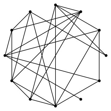
Figure 1. A realization of the Erdős-Rényi random graph with $n=12$ and $p=\tfrac{1}{3}$.

Each vertex carries an Ising spin that can take the values $-1$ or $+1$. Let $S_{n}=\left\{-1,+1\right\}^{V}$ denote the set of spin configurations on $V$, and let $H_{n}$ be the Hamiltonian on $S_{n}$ defined by

(1.1) $$H_{n}\left(\sigma\right)=-\frac{1}{n}\sum_{\left(v,w\right)\in E}\sigma(v)\sigma(w)-h\sum_{v\in V}\sigma(v),\quad\sigma\in S_{n}.$$

In other words, single spins interact with an external magnetic field $h\in(0,\infty)$, while pairs of neighbouring spins interact with each other with a ferromagnetic coupling strength $1/n$.

Let $\boxminus=\left\{-1\right\}^{V}$ and $\boxplus=\left\{+1\right\}^{V}$ denote the configuration where all spins are $-1$, respectively, $+1$. Since

(1.2) $$H_{n}\left(\boxminus\right)=-\frac{\left|E\right|}{n}+hn,$$

we have the geometric representation

(1.3) $$H_{n}\left(\sigma\right)=H_{n}\left(\boxminus\right)+\frac{2}{n}\left|\partial_{E}\sigma\right|-2h\left|\sigma\right|,\quad\sigma\in S_{n},$$

where

(1.4) $$\partial_{E}\sigma=\left\{\left(v,w\right)\in E\colon\sigma(v)=-\sigma(w)=+1\right\}$$

is the edge-boundary of $\sigma$ and

(1.5) $$\left|\sigma\right|=\left\{v\in\mathrm{ER}_{n}(p)\colon\,\sigma(v)=+1\right\}$$

is the vertex-volume of $\sigma$.

In the present paper we consider a spin-flip dynamics on $S_{n}$ commonly referred to as Glauber dynamics, defined as the continuous-time Markov process with transition rates

(1.6) $$r\left(\sigma,\sigma\right)=\begin{cases}e^{-\beta[H_{n}(\sigma^{\prime})-H_{n}(\sigma)]_{+}},&\mbox{if }\left\|\sigma-\sigma^{\prime}\right\|=2,\\ 0,&\mbox{if }\left\|\sigma-\sigma^{\prime}\right\|>2,\end{cases}\quad\sigma,\sigma^{\prime}\in S_{n},$$

where $\|\cdot\|$ is the $\ell_{1}$-norm on $S_{n}$. This dynamics has as reversible stationary distribution the Gibbs measure

(1.7) $$\mu_{n}\left(\sigma\right)=\frac{1}{Z_{n}}e^{-\beta H_{n}(\sigma)},\quad\sigma\in S_{n},$$

where $\beta\in(0,\infty)$ is the inverse temperature and $Z_{n}$ is the normalizing partition sum. We write

(1.8) $$\left\{\xi_{t}\right\}_{t\geq 0}$$

to denote the path of the random dynamics and $\mathbb{P}_{\xi}$ to denote its law given $\xi_{0}=\xi$. For $\chi\subset S_{n}$, we write

(1.9) $$\tau_{\chi}=\inf\{t\geq 0\colon\,\xi_{t}\in\chi,\,\xi_{t-}\notin\chi\}.$$

to denote the first hitting/return time of $\chi$.

We define the magnetization of $\sigma$ by

(1.10) $$m\left(\sigma\right)=\frac{1}{n}\sum_{v\in V}\sigma(v),$$

and observe the relation

(1.11) $$m\left(\sigma\right)=\frac{2\left|\sigma\right|}{n}-1,\quad\sigma\in S_{n}.$$

We will frequently switch between working with volume and working with magnetization. Equation (1.11) ensures that these are in one-to-one correspondence. Accordingly, we will frequently look at the dynamics from the perspective of the induced volume process and magnetization process,

(1.12) $$\left\{\left|\xi_{t}\right|\right\}_{t\geq 0},\quad\left\{m(\xi_{t})\right\}_{t\geq 0},$$

which are not Markov.

1.3. Metastable pair

For fixed $n$, the Hamiltonian in (1.1) achieves a global minimum at $\boxplus$ and a local minimum at $\boxminus$. In fact, $\boxminus$ is the deepest local minimum not equal to $\boxplus$ (at least for $h$ small enough). However, in the limit as $n\to\infty$, these do not form a metastable pair of configurations because entropy comes into play.

Definition 1.1 (Metastable regime).

The parameters $\beta,h$ are said to be in the metastable regime when

(1.13) $$\beta\in(1/p,\infty),\qquad h\in\big{(}0,p\chi(\beta p)\big{)}$$

with (see Fig. 2)

(1.14) $$\chi(\lambda)=\sqrt{1-\tfrac{1}{\lambda}}-\tfrac{1}{2\lambda}\log\left[\lambda\left(1+\sqrt{1-\tfrac{1}{\lambda}}\,\right)^{2}\right],\qquad\lambda\geq 1.$$

Figure 2. Plot of $\lambda\mapsto\chi(\lambda)$.

We have $\lim_{\lambda\to\infty}\chi(\lambda)=1$ and $\lim_{\lambda\downarrow 1}\chi(\lambda)=0$ (with slope $\tfrac{1}{2}$). Hence, for $\beta\to\infty$ any $h\in(0,p)$ is metastable, while for $\beta\downarrow 1/p$ or $p\downarrow 0$ no $h\in(0,\infty)$ is metastable. The latter explains why we do not consider the non-dense Erdős-Rényi random graph with $p=p_{n}\downarrow 0$ as $n\to\infty$. $\blacksquare$

The threshold $\beta_{c}=1/p$ is the critical temperature: the static model has a phase transition at $h=0$ when $\beta>\beta_{c}$ and no phase transition when $\beta\leq\beta_{c}$ (see e.g. Dommers, Giardinà and van der Hofstad [8]).

To define the proper metastable pair of configurations, we need the following definitions. Let

(1.15) $$\Gamma_{n}=\{-1,-1+\tfrac{2}{n},\ldots,1-\tfrac{2}{n},1\},\quad I_{n}(a)=-\frac{1}{n}\log\binom{n}{\tfrac{1+a}{2}n},\quad J_{n}(a)=2\beta(pa+h)-2I^{\prime}_{n}(a).$$

Define

(1.16) $$\mathbf{m}_{n} =\min\left\{a\in\Gamma_{n}\colon\,J_{n}(a)\leq 0\right\},$$

$$\mathbf{t}_{n} =\min\left\{a\in\Gamma_{n}\colon\,a>\mathbf{m}_{n},\,J_{n}(a)\geq 0\right\},$$

$$\mathbf{s}_{n} =\min\left\{a\in\Gamma_{n}\colon\,a>\mathbf{t}_{n},\,J_{n}(a)\leq 0\right\}.$$

The numbers in the left-hand side of (1.16) play the role of magnetizations; it will be made clear below that when in the metastable regime, these quantities are well defined. Further define

(1.17) $$\mathbf{M}_{n}=\frac{n}{2}(\mathbf{m}_{n}+1),\quad\mathbf{T}_{n}=\frac{n}{2}(\mathbf{t}_{n}+1),\quad\mathbf{S}_{n}=\frac{n}{2}(\mathbf{s}_{n}+1),$$

which are the volumes corresponding to (1.16), and

(1.18) $$A_{k}=\left\{\sigma\in S_{n}\colon\,\left|\sigma\right|=k\right\},\qquad k\in\{0,1,\ldots,n-1,n\},$$

the set of configurations with volume $k$. Define

(1.19) $$R_{n}(a)=-\frac{1}{2}pa^{2}-ha+\frac{1}{\beta}I_{n}(a)$$

and note that

(1.20) $$R^{\prime}_{n}(a)=-pa-h+\frac{1}{\beta}I^{\prime}_{n}(a)=-\frac{1}{2\beta}J_{n}(a).$$

The motivation behind the definitions in (1.15), (1.16) and (1.19) will become clear in Section 2. Via Stirling’s formula it follows that

(1.21) $$J_{n}(a)=2\beta(pa+h)+\log\left(\frac{1-a+\frac{1}{n}}{1+a+\frac{1}{n}}\right)+O(n^{-2}),\quad a\in\Gamma_{n}.$$

We will see that, in the limit as $n\to\infty$ when $(\beta,h)$ is in the metastable regime defined by (1.13), the numbers in (1.16) are well-defined: $A_{\mathbf{M}_{n}}$ is the metastable set, $A_{\mathbf{S}_{n}}$ is the stable set, $A_{\mathbf{T}_{n}}$ is the top set, i.e., the set of saddle points that lie in between $A_{\mathbf{M}_{n}}$ and $A_{\mathbf{S}_{n}}$. Our key object of interest will be the crossover time from $A_{\mathbf{M}_{n}}$ to $A_{\mathbf{S}_{n}}$ via $A_{\mathbf{T}_{n}}$.

Note that

(1.22) $$\Gamma_{n}\to[-1,1],\quad I_{n}(a)\to I(a),\quad J_{n}(a)\to J_{p,\beta,h}(a),\qquad n\to\infty,$$

with

(1.23) $$J_{p,\beta,h}(a)=2\beta(pa+h)+\log\left(\frac{1-a}{1+a}\right)$$

and

(1.24) $$I(a)=\frac{1-a}{2}\log\left(\frac{1-a}{2}\right)+\frac{1+a}{2}\log\left(\frac{1+a}{2}\right).$$

Accordingly,

(1.25) $$\mathbf{m}_{n}\to\mathbf{m},\quad\mathbf{t}_{n}\to\mathbf{t},\quad\mathbf{s}_{n}\to\mathbf{s},\qquad n\to\infty,$$

with $\mathbf{m}$, $\mathbf{t}$, $\mathbf{s}$ the three successive zeroes of $J$ (see Fig. 4 and recall (1.16)). Define

(1.26) $$R_{p,\beta,h}(a)=-\frac{1}{2}pa^{2}-ha+\frac{1}{\beta}I(a)$$

Note that $R_{p,\beta,h}(a)$ plays the role of free energy: $-\frac{1}{2}pa^{2}-ha$ and $\frac{1}{\beta}I(a)$ represent the energy, respectively, entropy at magnetisation $a$. Note that $I(a)$ equals the relative entropy of the probability measure $\tfrac{1}{2}(1+a)\delta_{+1}+\tfrac{1}{2}(1-a)\delta_{-1}$ with respect to the counting measure $\delta_{+1}+\delta_{-1}$. Also note that

(1.27) $$R^{\prime}_{p,\beta,h}(a)=-pa-h+\frac{1}{\beta}I^{\prime}(a)=-\frac{1}{2\beta}J_{p,\beta,h}(a).$$

Remark 1.2.

As shown in Corollary 3.6 below, if $h\in(p,\infty)$, then (1.6) leads to non-metastable behaviour where the dynamics ‘drifts’ through a sequence of configurations with volume growing from $\mathbf{M}$ to $\mathbf{S}$ within time $O(1)$. $\blacksquare$

1.4. Metastability on $K_{n}$

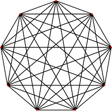
Figure 3. The complete graph with $n=9$.

Let $K_{n}$ be the complete graph on $n$ vertices (see Fig. 3). Spin-flip dynamics on $K_{n}$, commonly referred to as Glauber dynamics for the Curie-Weiss model, is defined as in Section 1.2 but with the Curie-Weiss Hamiltonian

(1.28) $$H_{n}(\sigma)=-\frac{1}{2n}\sum_{1\leq i,j\leq n}\sigma(i)\sigma(j)-h\sum_{1\leq i\leq n}\sigma(i),\quad\sigma\in S_{n}.$$

This is the special case of (1.1) when $p=1$, except for the diagonal term $-\frac{1}{2n}\sum_{1\leq i\leq n}\sigma(i)\sigma(i)=-\tfrac{1}{2}$, which shifts $H_{n}$ by a constant and has no effect on the dynamics. The advantage of (1.28) is that we may write

(1.29) $$H_{n}(\sigma)=n\big{[}-\tfrac{1}{2}m(\sigma)^{2}-hm(\sigma)\big{]},$$

which shows that the energy is a function of the magnetization only, i.e., the Curie-Weiss model is a mean-field model. Clearly, this property fails on $\mathrm{ER}_{n}(p)$.

For the Curie-Weiss model it is known that there is a critical inverse temperature $\beta_{c}=1$ such that, for $\beta>\beta_{c}$, $h$ small enough and in the limit as $n\to\infty$, the stationary distribution $\mu_{n}$ given by (1.7) and (1.28) has two phases: the ‘minus-phase’, where the majority of the spins are $-1$, and the ‘plus-phase’, where the majority of the spins are $+1$. These two phases are the metastable state, respectively, the stable state for the dynamics. In the limit as $n\to\infty$, the dynamics of the magnetization introduced in (1.12) (which is Markov) converges to a Brownian motion on $[-1,+1]$ in the double-well potential $a\mapsto R_{1,\beta,h}(a)$ (see Fig. 4).

Figure 4. Plot of $R_{p,\beta,h}(a)$ as a function of the magnetization $a$. The metastable set $A_{\mathbf{M}}$ has magnetization $\mathbf{m}<0$, the stable set $A_{\mathbf{S}}$ has magnetization $\mathbf{s}>0$, the top set has magnetization $\mathbf{t}<0$. Note that $R_{p,\beta,h}(-1)=-\tfrac{1}{2}p+h$, $R_{p,\beta,h}(0)=-\beta^{-1}\log 2$, $R_{p,\beta,h}(+1)=-\tfrac{1}{2}p-h$ and $R_{p,\beta,h}^{\prime}(-1)=-\infty$, $R_{p,\beta,h}^{\prime}(0)=-h$, $R_{p,\beta,h}^{\prime}(+1)=\infty$.

The following theorem can be found in Bovier and den Hollander [4, Chapter 13]. For $p=1$, the metastable regime in (1.13) becomes

(1.30) $$\beta\in(1,\infty),\qquad h\in\big{(}0,\chi(\beta)\big{)}.$$

Theorem 1.3 (Average crossover time on $K_{n}$).

Subject to (1.30), as $n\to\infty$, uniformly in $\xi\in A_{\mathbf{M}_{n}}$,

(1.31) $$\mathbb{E}_{\xi}\left[\tau_{A_{\mathbf{S}_{n}}}\right]=[1+o_{n}(1)]\,\frac{\pi}{1+\mathbf{t}}\sqrt{\frac{1-\mathbf{t}^{2}}{1-\mathbf{m}^{2}}}\frac{1}{\beta\sqrt{R_{1,\beta,h}^{\prime\prime}(\mathbf{m})[-R_{1,\beta,h}^{\prime\prime}(\mathbf{t})]}}\,e^{\beta n[R_{1,\beta,h}(\mathbf{t})-R_{1,\beta,h}(\mathbf{m})]}.$$

Fig. 4 illustrates the setting: the average crossover time from $A_{\mathbf{M}_{n}}$ to $A_{\mathbf{S}_{n}}$ depends on the energy barrier $R_{1,\beta,h}(\mathbf{t})-R_{1,\beta,h}(\mathbf{m})$ and on the curvature of $R_{1,\beta,h}$ at $\mathbf{m}$ and $\mathbf{t}$. Note that $\mathbf{m},\mathbf{s},\mathbf{t}$ in Fig. 4 are the limits as $n\to\infty$ of $\mathbf{m}_{n},\mathbf{s}_{n},\mathbf{t}_{n}$ defined in (1.16) for $p=1$.

1.5. Metastability on $\mathrm{ER}_{n}(p)$

Unlike for the spin-flip dynamics on $K_{n}$, the induced processes defined in (1.12) are not Markovian. This is due to the random geometry of $\mathrm{ER}_{n}(p)$. However, we will see that they are almost Markovian, a fact that we will exploit by comparing the dynamics on $\mathrm{ER}_{n}(p)$ with that on $K_{n}$, but with a ferromagnetic coupling strength $p/n$ rather than $1/n$ and with an external magnetic field that is a small perturbation of $h$.

As shown in Lemma 2.2 below, in the metastable regime the function $a\mapsto R_{p}(a)$ has a double-well structure just like in Fig. 4, so that the metastable state $A_{\mathbf{M}}$ and the stable state $A_{\mathbf{S}}$ are separated by an energy barrier represented by $A_{\mathbf{T}}$.

We are finally in a position to state our main theorem.

Theorem 1.4 (Average crossover time on $\mathrm{ER}_{n}(p)$).

Subject to (1.30), with $\mathbb{P}_{\mathrm{ER}_{n}(p)}$-probability tending to $1$ as $n\to\infty$, and uniformly in $\xi\in A_{\mathbf{M}_{n}}$,

(1.32) $$\mathbb{E}_{\xi}\left[\tau_{A_{\mathbf{S}_{n}}}\right]=n^{E_{n}}\,e^{\beta n[R_{p,\beta,h}(\mathbf{t})-R_{p,\beta,h}(\mathbf{m})]}$$

where the random exponent $E_{n}$ satisfies

(1.33) $$\lim_{n\to\infty}\mathbb{P}_{\mathrm{ER}_{n}(p)}\big{(}|E_{n}|\leq\beta(\mathbf{t}-\mathbf{m})\tfrac{11}{6}\big{)}=1.$$

Thus, apart from a polynomial error term, the average crossover time is the same as on the complete graph with ferromagnetic interaction strength $p/n$ instead of $1/n$.

1.6. Discussion and outline

We discuss the significance of our main theorem.

1. Theorem 1.4 provides an estimate on the average crossover time from $A_{\mathbf{M}_{n}}$ to $A_{\mathbf{S}_{n}}$ on $\mathrm{ER}_{n}(p)$ (recall Fig. 4). The estimate is uniform in the starting configuration. The exponential term in the estimate is the same as on $K_{n}$, but with a ferromagnetic interaction strength $p/n$ rather than $1/n$. The multiplicative error term is at most polynomial in $n$. Such an error term is not present on $K_{n}$, for which the prefactor is known to be a constant up to a multiplicative factor $1+o(1)$ (as shown in Theorem 1.3). The randomness of $\mathrm{ER}_{n}(p)$ manifests itself through a more complicated prefactor, which we do not know how to identify. What is interesting is that, apparently, $\mathrm{ER}_{n}(p)$ is so homogeneous for large $n$ that the prefactor is at most polynomial. We expect the prefactor to be random under the law $\mathbb{P}_{\mathrm{ER}_{n}(p)}$.

2. It is known that on $K_{n}$ the crossover time divided by it average has an exponential distribution in the limit as $n\to\infty$, as is typical for metastable behaviour. The same is true on $\mathrm{ER}_{n}(p)$. A proof of this fact can be obtained in a straightforward manner from the comparison properties underlying the proof of Theorem 1.4. These comparison properties, which are based on coupling of trajectories, also allow us to identify the typical set of trajectories followed by the spin-flip dynamics prior to the crossover. We will not spell out the details.

3. The proof of Theorem 1.4 is based on estimates of transition probabilities and transition times between pairs of configurations with different volume, in combination with a coupling argument. Thus we are following the path-wise approach to metastabuilty (see [4] for background). Careful estimates are needed because on $\mathrm{ER}_{n}(p)$ the processes introduced in (1.12) are not Markovian, unlike on $K_{n}$.

4. Bovier, Marello and Pulvirenti [5] use capacity estimates and concentration of measure estimates to show that the prefactors form a tight family of random variables under the law $\mathbb{P}_{\mathrm{ER}_{n}(p)}$ as $n\to\infty$, which constitutes a considerable sharpening of (1.32). The result is valid for $\beta>\beta_{c}$ and $h$ small enough. The starting configuration is not arbitrary, but is drawn according to the last-exit-biased distribution for the transition from $A_{\mathbf{M}_{n}}$ to $A_{\mathbf{S}_{n}}$, as is common in the potential-theoretic approach to metastability. The exponential limit law is therefore not immediate.

5. Another interesting model is where the randomness sits in the vertices rather than in the edges, namely, Glauber spin-flip dynamics with Hamiltonian

(1.34) $$H_{n}(\sigma)=-\frac{1}{n}\sum_{1\leq i,j\leq n}\sigma(i)\sigma(j)-\sum_{1\leq i\leq n}h_{i}\sigma(i),$$

where $h_{i}$, $1\leq i\leq n$, are i.i.d. random variables drawn from a common probability distribution $\nu$ on $\mathbb{R}$. The metastable behaviour of this model was analysed in Bovier et al. [3] (discrete $\nu$) and Bianchi et al. [1] (continuous $\nu$). In particular, the prefactor was computed up to a multiplicative factor $1+o(1)$, and turns out to be rather involved (see [4, Chapters 14–15]). Our model is even harder because the interaction between the spins runs along the edges of $\mathrm{ER}_{n}(p)$, which has an intricate spatial structure. Consequently, the so-called lumping technnique (employed in [3] and [1] to monitor the magnetization on the level sets of the magnetic field) can no longer be used. For the dynamics under (1.34) the exponential law was proved in Bianchi et al. [2].

Outline. The remainder of the paper is organized as follows. In Section 2 we define the perturbed spin-flip dynamics on $K_{n}$ (Definition 2.1 below) and explain why Definition 1.1 identifies the metastable regime (Lemma 2.2 below). In Section 3 we collect a few basic facts about the geometry of $\mathrm{ER}_{n}(p)$ and the spin-flip dynamics on $\mathrm{ER}_{n}(p)$. In Section 4 we derive rough capacity estimates for the spin-flip dynamics on $\mathrm{ER}_{n}(p)$. In Section 5 we derive refined capacity estimates. In Section 6 we show that two copies of the spin-flip dynamics starting near the metastable state can be coupled in a short time. In Section 7, finally, we prove Theorem 1.4.

2. Preparations

In Section 2.1 we define the perturbed spin-flip dynamics on $K_{n}$ that will be used as comparison object. In Section 2.2 we do a rough metastability analysis of the perturbed model. In Section 2.3 we show that $R_{p,\beta,h}$ has a double-well structure if and only if $(\beta,h)$ is in the metastable regime, in the sense of Definition 1.1 (Lemma 2.2 below).

Define

(2.1) $$J^{*}_{n}(a)=2\beta\left(p\left(a+\tfrac{2}{n}\right)+h\right)+\log\left(\frac{1-a}{1+a+\frac{2}{n}}\right),\quad a\in\Gamma_{n}.$$

We see from (1.21) that $J_{n}(a)=J^{*}_{n}(a)+O(n^{-2})$ when $\beta p=\frac{1}{1-a^{2}}$. This will be useful for the analysis of the ‘free energy landscape’.

2.1. Perturbed Curie-Weiss

We will compare the dynamics on $\mathrm{ER}_{n}(p)$ with that on $K_{n}$, but with a ferromagnetic coupling strength $p/n$ rather than $1/n$, and with an external magnetic field field that is a small perturbation of $h$.

Definition 2.1 (Perturbed Curie-Weiss).

(1) Let

(2.2) $$H_{n}^{u}\left(\sigma\right) = -\tfrac{p}{2n}\sum_{1\leq i,j\leq n}\sigma(i)\sigma(j)-h_{n}^{u}\sum_{1\leq i\leq n}\sigma(i),\quad\sigma\in S_{n},$$

(2.3) $$H_{n}^{l}\left(\sigma\right) = -\tfrac{p}{2n}\sum_{1\leq i,j\leq n}\sigma(i)\sigma(j)-h_{n}^{l}\sum_{1\leq i\leq n}\sigma(i),\quad\,\sigma\in S_{n},$$

be the Hamiltonians on $S_{n}$ corresponding to the Curie-Weiss model on $n$ vertices with ferromagnetic coupling strength $p/n$, and with external magnetic fields $h_{n}^{u}$ and $h_{n}^{l}$ given by

(2.4) $$h_{n}^{u}=h+\tfrac{\left(1+\epsilon\right)\log(n^{11/6})}{n},\qquad h_{n}^{l}=h-\tfrac{\left(1+\epsilon\right)\log(n^{11/6})}{n},$$

where $\epsilon>0$ is arbitrary. The indices $u$ and $l$ stand for upper and lower, and the choice of exponent $\tfrac{11}{6}$ will become clear in Section 4.
(2) The equilibrium measures on $S_{n}$ corresponding to (2.2) and (2.3) are denoted by $\mu_{n}^{u}$ and $\mu_{n}^{l}$, respectively (recall (1.7)).
(3) The Glauber dynamics based on (2.2) and (2.3) are denoted by

(2.5) $$\left\{\xi_{t}^{u}\right\}_{t\geq 0},\qquad\left\{\xi_{t}^{l}\right\}_{t\geq 0},$$

respectively.
(4) The analogues of (1.16) and (1.17) are denoted by $\mathbf{m}^{u}_{n},\mathbf{t}^{u}_{n},\mathbf{s}^{u}_{n}$, $\mathbf{M}^{u}_{n},\mathbf{T}^{u}_{n},\mathbf{S}^{u}_{n}$ and $\mathbf{m}^{l}_{n},\mathbf{t}^{l}_{n},\mathbf{s}^{l}_{n}$, $\mathbf{M}^{l}_{n},\mathbf{T}^{l}_{n},\mathbf{S}^{l}_{n}$, respectively. $\blacksquare$

In what follows we will suppress the $n$-dependence from most of the notation. Almost all of the analysis in Sections 2–7 pertains to the dynamics on $\mathrm{ER}_{n}(p)$.

2.2. Metastability for perturbed Curie-Weiss

Recall that $\{\xi_{t}^{u}\}_{t\geq 0}$ and $\{\xi_{t}^{l}\}_{t\geq 0}$ denote the Glauber dynamics for the Curie-Weiss model driven by (2.2) and (2.3), respectively. An important feature is that their magnetization processes

(2.6) $$\ \left\{\theta_{t}^{u}\right\}_{t\geq 0} =\{m(\xi_{\tau_{s}^{l}}^{l})\}_{t\geq 0}$$

$$\left\{\theta_{t}^{l}\right\}_{t\geq 0} =\{m(\xi_{\tau_{s}^{u}}^{u})\}_{t\geq 0}$$

are continuous-time Markov processes themselves (see e.g. Bovier and den Hollander [4, Chaper 13]). The state space of these two processes is $\Gamma_{n}=\left\{-1,-1+\frac{2}{n},\ldots,1-\frac{2}{n},1\right\}$, and the transition rates are

(2.7) $$q^{u}\left(a,a^{\prime}\right)=\begin{cases}\frac{n}{2}\left(1-a\right)e^{-\beta[p(-2a-\frac{2}{n})-2h^{u}]_{+}},&\mbox{if }a^{\prime}=a+\frac{2}{n},\\ \frac{n}{2}\left(1+a\right)e^{-\beta[p(2a+\frac{2}{n})+2h^{u}]_{+}},&\mbox{if }a^{\prime}=a-\frac{2}{n},\\ 0,&\mbox{otherwise},\end{cases}$$

(2.8) $$q^{l}\left(a,a^{\prime}\right)=\begin{cases}\frac{n}{2}\left(1-a\right)e^{-\beta[p(-2a-\frac{2}{n})-2h^{l}]_{+}},&\mbox{if }a^{\prime}=a+\frac{2}{n},\\ \frac{n}{2}\left(1+a\right)e^{-\beta[p(2a+\frac{2}{n})+2h^{l}]_{+}},&\mbox{if }a^{\prime}=a-\frac{2}{n},\\ 0,&\mbox{otherwise},\end{cases}$$

respectively. The processes in (2.6) are reversible with respect to the Gibbs measures

(2.9) $$\nu^{u}\left(a\right) = \frac{1}{z^{u}}e^{\beta n(\tfrac{1}{2}pa^{2}+h^{u}a)}{n\choose\frac{1+a}{2}n},\quad a\in\Gamma_{n},$$

(2.10) $$\nu^{l}\left(a\right) = \frac{1}{z^{l}}e^{\beta n(\tfrac{1}{2}pa^{2}+h^{l}a)}{n\choose\frac{1+a}{2}n},\quad a\in\Gamma_{n},$$

respectively.

Define

(2.11) $$\Psi^{u}\left(a\right) = -\tfrac{1}{2}pa^{2}-h^{u}a,\quad a\in\Gamma_{n},$$

(2.12) $$\Psi^{l}(a) = -\tfrac{1}{2}pa^{2}-h^{l}a,\quad a\in\Gamma_{n}.$$

Note that (2.7) and (2.9) can be written as

$$q^{u}\left(a,a+\tfrac{2}{n}\right) = \tfrac{n}{2}\left(1-a\right)e^{-\beta n[\Psi^{u}(a+\tfrac{2}{n})-\Psi^{u}(a)]_{+}},$$

(2.13) $$\nu^{u}\left(a\right) = \frac{1}{z^{u}}e^{-\beta n\Psi^{u}(a)}{n\choose\frac{n}{2}\left(1+a\right)},$$

and similar formulas hold for (2.8) and (2.10). The properties of the function $\nu^{u}\colon\Gamma_{n}\to\left[0,1\right]$ can be analysed by looking at the ratio of adjacent values:

(2.14) $$\frac{\nu^{u}\left(a+\tfrac{2}{n}\right)}{\nu^{u}\left(a\right)}=\exp\left(2\beta\left(p\left(a+\tfrac{2}{n}\right)+h^{u}\right)+\log\Big{(}\tfrac{1-a}{1+a+\tfrac{2}{n}}\Big{)}\right),$$

which suggests that ‘local free energy wells’ in $\nu^{u}$ can be found by looking at where the sign of

(2.15) $$2\beta\left(p\left(a+\tfrac{2}{n}\right)+h^{u}\right)+\log\left(\tfrac{1-a}{1+a+\frac{2}{n}}\right)$$

changes from negative to positive. To that end note that, in the limit $n\to\infty$, the second term is positive for $a<0$, tends to $\infty$ as $a\to-1$, is negative for $a\geq 0$, tends to $-\infty$ as $a\to 1$, and tends to $0$ as $a\to 0$. The first term is linear in $a$, and for appropriate choices of $p$, $\beta$ and $h^{u}$ (see Definition 1.1) is negative near $a=-1$ and becomes positive at some value $a<0$. This implies that, for appropriate choices of $p$, $\beta$ and $h^{u}$, the sum of the two terms in (2.15) can change sign $+\to-\to+$ on the interval $\left[-1,0\right]$, and can change sign $+\to-$ on $\left[0,1\right]$. Assuming that our choice of $p$, $\beta$ and $h^{u}$ corresponds to this change-of-signs sequence, we define $\mathbf{m}^{u}$, $\mathbf{t}^{u}$ and $\mathbf{s}^{u}$ as in (1.16) with $h$ replaced by $h^{u}$. This observation makes it clear that the sets in the right-hand side of (1.16) indeed are non-empty.

The interval $\left[\mathbf{m}^{u},\mathbf{t}^{u}\right]$ poses a barrier for the process $\{\theta_{t}^{u}\}_{t\geq 0}$ due to a negative drift, which delays the initiation of the convergence to equilibrium while the process passes through the interval $\left[\mathbf{t}^{u},\mathbf{s}^{u}\right]$. The same is true for the process $\{\xi_{t}^{u}\}_{t\geq 0}$. Similar observations hold for $\{\theta_{t}^{l}\}_{t\geq 0}$ and $\{\xi_{t}^{l}\}_{t\geq 0}$. Recall Fig. 4.

2.3. Double-well structure

Lemma 2.2 (Metastable regime).

The potential $R_{p,\beta,h}$ defined in (1.26) has a double-well structure if and only if $\beta p>1$ and $0<h<p\chi(\beta p)$, with $\chi$ defined in (1.14).

Proof.

In order for $R_{p,\beta,h}$ to have a double-well structure, the measure $\nu$ must have two distinct maxima on the interval $\left(-1,1\right)$. From (1.22), (1.27) and (2.14) it follows that

(2.16) $$J_{p,\beta,h}(a)=2\lambda\left(a+\tfrac{h}{p}\right)+\log\left(\tfrac{1-a}{1+a}\right),\qquad\lambda=\beta p,$$

must have one local minimum and two zeroes in $\left(-1,1\right)$. Since

(2.17) $$J_{p,\beta,h}^{\prime}(a)=2\left(\lambda-\tfrac{1}{1-a^{2}}\right),\qquad a\in[-1,1],$$

it must therefore be that $\lambda>1$. The local minimum is attained when

(2.18) $$\lambda=\tfrac{1}{1-a^{2}},$$

i.e., when $a=a_{\lambda}=-\sqrt{1-\frac{1}{\lambda}}$ ($a_{\lambda}$ must be negative because it lies in $(\mathbf{m},\mathbf{t})$; recall Fig. 4). Since

(2.19) $$0>J_{p,\beta,h}(a_{\lambda})=2\lambda\left(a_{\lambda}+\tfrac{h}{p}\right)+\log\left(\tfrac{1-a_{\lambda}}{1+a_{\lambda}}\right),$$

it must therefore be that

(2.20) $$\tfrac{h}{p}<\chi(\lambda)$$

with $\chi(\lambda)$ given by (1.14). ∎

3. Basic facts

In this section we collect a few facts that will be needed in Section 4 to derive capacity estimates for the dynamics on $\mathrm{ER}_{n}(p)$. In Section 3.1 we derive a large deviation bound for the degree of typical vertices $\mathrm{ER}_{n}(p)$ (Lemma 3.2 below). In Section 3.2 we do the same for the edge-boundary of typical configurations (Lemma 3.3 below). In Section 3.3 we derive upper and lower bounds for the jump rates of the volume process (Lemmas 3.4–3.5 and Corollary 3.6 below), and show that the return times to the metastable set conditional on not hitting the top set are small (Lemma 3.7 below). In Section 3.4 we use the various bounds to show that the probability for the volume process to grow by $n^{1/3}$ is almost uniform in the starting configuration (Lemma 3.8 and Corollary 3.9 below).

Definition 3.1 (Notation).

For a vertex $v\in V$, we will write $v\in\sigma$ to mean $\sigma(v)=+1$ and $v\notin\sigma$ to mean $\sigma(v)=-1$. Similarly, we will denote by $\overline{\sigma}$ the configuration obtained from $\sigma$ by flipping the spin at every vertex, i.e., $\sigma(v)=+1$ if and only if $\overline{\sigma}(v)=-1$. For two configurations $\sigma,\sigma^{\prime}$ we will say that $\sigma\subseteq\sigma^{\prime}$ if and only if $v\in\sigma\implies v\in\sigma^{\prime}$. By $\sigma\cup\sigma^{\prime}$ we denote the configuration satisfying $v\in\sigma\cup\sigma^{\prime}$ if and only if $v\in\sigma$ or $v\in\sigma^{\prime}$. A similar definition applies to $\sigma\cap\sigma^{\prime}$. We will also write $\sigma\sim\sigma^{\prime}$ when there is a $v\in V$ such that $\sigma=\sigma^{\prime}\cup\left\{v\right\}$ or $\sigma^{\prime}=\sigma\cup\left\{v\right\}$. We will say that $\sigma$ and $\sigma^{\prime}$ are neighbours. We write $\deg(v)$ for the degree of $v\in V$. $\blacksquare$

3.1. Concentration bounds for $\mathrm{ER}_{n}(p)$

Recall that $\mathbb{P}_{\mathrm{ER}_{n}(p)}$ denotes the law $\mathrm{ER}_{n}(p)$.

Lemma 3.2 (Concentration of degrees and energies).

With $\mathbb{P}_{\mathrm{ER}_{n}(p)}$-probability tending to $1$ as $n\to\infty$ the following is true. For any $\epsilon>0$ and any $c>\sqrt{\frac{1}{8}\log 2}$,

(3.1) $$pn-(1+\epsilon)\sqrt{n\log n}<\deg(v)<pn+(1+\epsilon)\sqrt{n\log n}\qquad\forall\,v\in V,$$

(3.2) $$\frac{1}{n}\left(2p|\xi|(n-|\xi|)-cn^{3/2}\right)-2h|\xi|\leq H_{n}(\xi)-H_{n}(\boxminus)$$

$$\qquad\qquad\qquad\leq\frac{1}{n}\left(2p|\xi|(n-|\xi|)+cn^{3/2}\right)-2h|\xi|\qquad\forall\,\xi\in S_{n}.$$

Proof.

These bounds are immediate from Hoeffding’s inequality and a union bound. ∎

3.2. Edge boundaries of $\mathrm{ER}_{n}(p)$

We partition the configuration space as

(3.3) $$S_{n}=\bigcup_{k=0}^{n}A_{k},$$

where $A_{k}$ is defined in (1.18). For $0\leq k\leq n$ and $-pk\left(n-k\right)\leq i\leq\left(1-p\right)k\left(n-k\right)$, define

(3.4) $$\phi_{i}^{k}=\left|\left\{\sigma\in A_{k}\colon\,\left|\partial_{E}\sigma\right|=pk\left(n-k\right)+i\right\}\right|,$$

i.e., $\phi_{i}^{k}$ counts the configurations $\sigma$ with volume $k$ whose edge-boundary size $\left|\partial_{E}\sigma\right|$ deviates by $i$ from its mean, which is equal to $pk\left(n-k\right)$. For $0\leq k\leq n$, let $\mathbb{P}_{k}$ denote the uniform distribution on $A_{k}$.

Lemma 3.3 (Upper bound on edge-boundary sizes).

With $\mathbb{P}_{\mathrm{ER}_{n}(p)}$-probability tending to $1$ as $n\to\infty$ the following are true. For $-pk(n-k)\leq j\leq(1-p)k(n-k)$ and $\varrho\colon\,\mathbb{N}\to\mathbb{R}_{+}$,

(3.5) $$\mathbb{P}_{k}\left[\phi_{j}^{k}\geq\varrho\left(n\right){n\choose k}p^{pk(n-k)+j}(1-p)^{(1-p)k(n-k)-j}{k(n-k)\choose pk(n-k)+j}\right]\leq\frac{1}{\varrho(n)}$$

and

(3.6) $$\mathbb{P}_{k}\left[\sum_{j\geq i}\phi_{j}^{k}\geq\varrho\left(n\right){n\choose k}e^{-\tfrac{2i^{2}}{k(n-k)}}\right] \leq\frac{1}{\varrho\left(n\right)},$$

$$\mathbb{P}_{k}\left[\sum_{j\leq-i}\phi_{j}^{k}\geq\varrho\left(n\right){n\choose k}e^{-\tfrac{2i^{2}}{k(n-k)}}\right] \leq\frac{1}{\varrho\left(n\right)}.$$

Proof.

Write $\simeq$ to denote equality in distribution. Note that if $\sigma\simeq\mathbb{P}_{k}$, then $\left|\partial_{E}\sigma\right|\simeq\mathrm{Bin}\left(k\left(n-k\right),p\right)$, and hence

(3.7) $$\mathbb{P}_{k}\left[\left|\partial_{E}\sigma\right|=i\right]=p^{i}\left(1-p\right)^{k\left(n-k\right)-i}{k\left(n-k\right)\choose i}.$$

In particular,

(3.8) $$\mathbb{E}_{k}\left[\phi_{j}^{k}\right]=\mathbb{E}_{k}\left[\sum_{\sigma\in A_{k}}\mathbbm{1}_{\left\{\left|\partial_{E}\sigma\right|=pk(n-k)+j\right\}}\right]={n\choose k}p^{pk(n-k)+j}(1-p)^{(1-p)k(n-k)-j}{k\left(n-k\right)\choose pk(n-k)+j}.$$

Hence, by Markov’s inequality, the claim in (3.5) follows. Moreover,

(3.9) $$\mathbb{E}_{k}\Bigg{[}\sum_{j\geq i}\phi_{j}^{k}\Bigg{]}=\mathbb{E}_{k}\left[\sum_{\sigma\in A_{k}}\mathbbm{1}_{\left\{\left|\partial_{E}\sigma\right|\geq pk(n-k)+i\right\}}\right]\\ \leq{n\choose k}e^{-2\tfrac{i^{2}}{k(n-k)}},$$

where we again use Hoeffding’s inequality. Hence, by Markov’s inequality, we get the first line in (3.6). The proof of the second line is similar. ∎

3.3. Jump rates for the volume process

The following lemma establishes bounds on the rate at which configurations in $A_{k}$ jump forward to $A_{k+1}$ and backward to $A_{k-1}$. In Appendix A we will sharpen the error in the prefactors in (3.10)–(3.11) from $2n^{2/3}$ to $O(1)$ and the error in the exponents in (3.10)–(3.11) from $3n^{-1/3}$ to $O(n^{-1/2})$. The formulas in (3.13) and (3.14) show that for small and large magnetization the rate forward, respectively, backward are maximal.

Lemma 3.4 (Bounds on forward jump rates).

With $\mathbb{P}_{\mathrm{ER}_{n}(p)}$-probability tending to $1$ as $n\to\infty$ the following are true.
(a) For $2n^{1/3}\leq k\leq n-2n^{1/3}$,

(3.10) $$\big{(}n-k-2n^{2/3}\big{)}e^{-2\beta[\vartheta_{k}+3n^{-1/3}]_{+}}$$

$$\qquad\leq\sum_{\xi\in A_{k+1}}r\left(\sigma,\xi\right)\leq\big{(}n-k-2n^{2/3}\big{)}e^{-2\beta[\vartheta_{k}-3n^{-1/3}]_{+}}+2n^{2/3},\qquad\sigma\in A_{k},$$

and

(3.11) $$\big{(}k-2n^{2/3}\big{)}e^{-2\beta[-\vartheta_{k}+3n^{-1/3}]_{+}}$$

$$\qquad\leq\sum_{\xi\in A_{k-1}}r\left(\sigma,\xi\right)\leq\big{(}k-2n^{2/3}\big{)}e^{-2\beta[-\vartheta_{k}-3n^{-1/3}]_{+}}+2n^{2/3},\qquad\sigma\in A_{k},$$

where

(3.12) $$\vartheta_{k}=p\left(1-\tfrac{2k}{n}\right)-h.$$

(b) For $n-\tfrac{n}{3}(p+h)\leq k<n$,

(3.13) $$\sum_{\xi\in A_{k+1}}r\left(\sigma,\xi\right)=n-k,\qquad\sigma\in A_{k}.$$

(c) For $0<k\leq\tfrac{n}{3}(p-h)$,

(3.14) $$\sum_{\xi\in A_{k-1}}r\left(\sigma,\xi\right)=k,\qquad\sigma\in A_{k}.$$

Proof.

The proof is via probabilistic counting.

(a) Write $\mathbb{P}$ for the law under which $\sigma\in S_{n}$ is a uniformly random configuration and $v\in\overline{\sigma}$ is a uniformly random vertex. By Hoeffding’s inequality, the probability that $v$ has more than $p\left|\sigma\right|+n^{2/3}$ neighbours in $\sigma$ (i.e., $w\in V$ such that $\left(v,w\right)\in E$ and $\sigma\left(w\right)=+1$) is bounded by

(3.15) $$\mathbb{P}\left[\left|E(v,\sigma)\right|\geq p\left|\overline{\sigma}\right|+n^{2/3}\right]\leq e^{-2n^{1/3}}.$$

where

(3.16) $$E(v,\sigma)=\left\{w\in\sigma\colon\,\left(v,w\right)\in E\right\}.$$

Define the event

(3.17) $$R^{+}\left(\sigma\right)=\left\{\exists\,\zeta\subseteq\overline{\sigma},\,\zeta\in A_{2n^{2/3}}\colon\,\left|E(v,\sigma)\right|\geq p\left|\sigma\right|+n^{2/3}\,\,\forall\,v\in\zeta,\right\},$$

i.e., the configuration $\overline{\sigma}$ has at least $2n^{2/3}$ vertices like $v$, each with at least $p\left|\sigma\right|+n^{2/3}$ neighbours in $\sigma$. Then, for $0\leq k\leq n-2n^{2/3}$,

(3.18) $$\mathbb{P}\left[R^{+}\left(\sigma\right)\right]\leq{\left|\overline{\sigma}\right|\choose 2n^{2/3}}\left(e^{-2n^{1/3}}\right)^{2n^{2/3}}\leq 2^{n}e^{-4n}.$$

Hence the probability that some configuration $\sigma\in S_{n}$ satisfies condition $R^{+}(\sigma)$ is bounded by

(3.19) $$\mathbb{P}\left[\bigcup_{\sigma\in S_{n}}R^{+}\left(\sigma\right)\right]\leq 4^{n}e^{-4n}\leq e^{-2n}.$$

Thus, with $\mathbb{P}_{\mathrm{ER}_{n}(p)}$-probability tending to $1$ as $n\to\infty$ there are no configurations $\sigma\in S_{n}$ satisfying condition $R^{+}(\sigma)$. The same holds for the event

(3.20) $$R^{-}\left(\sigma\right)=\left\{\exists\,\zeta\subseteq\overline{\sigma},\,\zeta\in A_{2n^{2/3}}\colon\,\left|E(v,\sigma)\right|\leq p\left|\sigma\right|-n^{2/3}\,\,\forall\,v\in\zeta\right\},$$

for which

(3.21) $$\mathbb{P}\left[\,\bigcup_{\sigma\in S_{n}}R^{-}\left(\sigma\right)\right]\leq e^{-2n}.$$

Now let $\sigma\in A_{k}$, and observe that $\sigma$ has $n-k$ neighbours in $A_{k+1}$ and $k$ neighbours in $A_{k-1}$. But if $\xi=\sigma\cup\left\{v\right\}\in A_{k+1}$, then by (1.3),

$$H_{n}\left(\xi\right)-H_{n}\left(\sigma\right) = \tfrac{2}{n}\Big{(}\left|E(v,\overline{\sigma})\right|-\left|E(v,\sigma)\right|\Big{)}-2h$$

$$= \tfrac{2}{n}\big{(}\deg\left(v\right)-2\left|E(v,\sigma)\right|\big{)}-2h$$

$$\leq \tfrac{2}{n}\big{(}pn+n^{1/2}\log n-2\left|E(v,\sigma)\right|\big{)}-2h,$$

where the last inequality uses (3.1) with $\varrho(n)=\log n$. Similarly,

(3.23) $$H_{n}\left(\xi\right)-H_{n}\left(\sigma\right) \geq \tfrac{2}{n}\left(pn-n^{1/2}\log n-2\left|E(v,\sigma)\right|\right)-2h.$$

The events $R^{+}(\sigma)$ in (3.17) and $R^{-}(\sigma)$ in (3.20) guarantee that for any configuration $\sigma$ at most $2n^{2/3}$ vertices in the configuration $\overline{\sigma}$ can have more than $n^{2/3}$ neighbours in $\sigma$. In other words, the configuration $\sigma$ has at most $2n^{2/3}$ neighbouring configurations in $A_{k+1}$ that differ in energy by more than $6n^{-1/3}-2h$. Since on the complement of $R^{+}(\sigma)$ with $\sigma\in A_{k}$ we have $|\{w\in\sigma\colon\,(v,w)\in E\}|\leq 2pk+2n^{1/3}$ (because $n^{1/2}\log n\leq n^{2/3}$ for $n$ large enough), from (3.19) and (3.21) we get that, with $\mathbb{P}_{\mathrm{ER}_{n}(p)}$-probability at least $1-e^{-2n}$,

(3.24) $$\left|\left\{\xi\in A_{k+1}\colon\,\xi\sim\sigma,\,H_{n}\left(\xi\right)-H_{n}\left(\sigma\right)\geq\tfrac{2}{n}\left(pn-2pk+3n^{2/3}\right)-2h\right\}\right|\leq 2n^{2/3},$$

$$\left|\left\{\xi\in A_{k+1}\colon\,\xi\sim\sigma,\,H_{n}\left(\xi\right)-H_{n}\left(\sigma\right)\leq\tfrac{2}{n}\left(pn-2pk-3n^{2/3}\right)-2h\right\}\right|\leq 2n^{2/3},$$

and hence, by (1.6), the rate at which the Markov chain starting at $\sigma\in A_{k}$ jumps to $A_{k+1}$ satisfies

(3.25) $$\sum_{\xi\in A_{k+1}}r\left(\sigma,\xi\right)\geq\big{(}n-k-2n^{2/3}\big{)}e^{-2\beta[\theta_{k}+3n^{-1/3}]_{+}},$$

(3.26) $$\sum_{\xi\in A_{k+1}}r\left(\sigma,\xi\right)\leq\big{(}n-k-2n^{2/3}\big{)}e^{-2\beta[\theta_{k}-3n^{-1/3}]_{+}}+2n^{2/3}.$$

Here the term $n-k-2n^{2/3}$ comes from exclusion of the at most $2n^{2/3}$ neighbours in configurations that differ from $\sigma$ in energy by more than $6n^{-1/3}-2h$. Similarly, with $\mathbb{P}_{\mathrm{ER}_{n}(p)}$-probability at least $1-e^{-2n}$,

(3.27) $$\left|\left\{\xi\in A_{k-1}\colon\,\xi\sim\sigma,\,H_{n}\left(\xi\right)-H_{n}\left(\sigma\right)\geq\tfrac{2}{n}\left(-pn+2pk+3n^{2/3}\right)+2h\right\}\right|\leq 2n^{2/3},$$

$$\left|\left\{\xi\in A_{k-1}\colon\,\xi\sim\sigma,\,H_{n}\left(\xi\right)-H_{n}\left(\sigma\right)\leq\tfrac{2}{n}\left(-pn+2pk-3n^{2/3}\right)+2h\right\}\right|\leq 2n^{2/3},$$

and hence, by (1.6), the rate at which the Markov chain starting at $\sigma\in A_{k}$ jumps to $A_{k-1}$ satisfies

(3.28) $$\sum_{\xi\in A_{k-1}}r\left(\sigma,\xi\right)\leq\big{(}k-2n^{2/3}\big{)}e^{-2\beta[-\theta_{k}-3n^{-1/3}]_{+}}+2n^{2/3},$$

(3.29) $$\sum_{\xi\in A_{k-1}}r\left(\sigma,\xi\right)\geq\big{(}k-2n^{2/3}\big{)}e^{-2\beta[-\theta_{k}+3n^{-1/3}]_{+}}.$$

This proves (3.10) and (3.11).

(b) To get (3.13), note that for $\xi=\sigma\cup\{v\}$ with $v\notin\sigma$,

$$H_{n}\left(\xi\right)-H_{n}\left(\sigma\right) = \tfrac{2}{n}\Big{(}\left|E(v,\overline{\sigma})\right|-\left|E(v,\sigma)\right|\Big{)}-2h$$

$$= \tfrac{2}{n}\Big{(}2\left|E(v,\sigma)\right|-\deg\left(v\right)\Big{)}-2h$$

$$\leq 2\left(2(n-k)-p+n^{-1/2}\log n-h\right)$$

for $n$ large enough, which is $\leq 0$ when $n-k\leq\tfrac{n}{3}(p+h)$, so that $r\left(\sigma,\xi\right)=1$ by (1.6).

(c) To get (3.14), note that for $\xi=\sigma\setminus\{v\}$ with $v\notin\sigma$,

$$H_{n}\left(\xi\right)-H_{n}\left(\sigma\right) = \tfrac{2}{n}\Big{(}\left|E(v,\sigma)\right|-\left|E(v,\overline{\sigma})\right|\Big{)}+2h$$

$$= \tfrac{2}{n}\Big{(}2\left|E(v,\sigma)\right|-\deg\left(v\right)\Big{)}+2h$$

$$\leq 2\left(2k-p+n^{-1/2}\log n+h\right)$$

for $n$ large enough, which is $\leq 0$ when $k\leq\tfrac{n}{3}(p-h)$, so that $r\left(\sigma,\xi\right)=1$ by (1.6). ∎

The following lemma is technical and merely serves to show that near $A_{\mathbf{M}}$ transitions involving a flip from $-1$ to $+1$ typically occur at rate 1.

Lemma 3.5 (Attraction towards the metastable state).

Suppose that $\left|\xi\right|=[1+o_{n}(1)]\,\mathbf{M}$. Then $r\left(\xi,\xi^{v}\right)=1$ for all but $O(n^{2/3})$ many $v\in\xi$.

Proof.

We want to show that

(3.32) $$H_{n}\left(\xi^{v}\right)<H_{n}\left(\xi\right)$$

for all but $O(n^{2/3})$ many $v\in\xi$. Note that by (3.20) and (3.21) there are at most $2n^{2/3}$ many $v\in\xi$ such that $|E(v,\overline{\xi})|\leq p(n-|\xi|)-n^{2/3}$, and at most $2n^{2/3}$ many $v\in\xi$ such that $|E(v,\xi)|\geq p|\xi|+n^{2/3}$. Hence, by (1.3), for all but at most $4n^{2/3}$ many $v\in\xi$ we have that

$$H_{n}\left(\xi^{v}\right) = H_{n}\left(\xi\right)+\tfrac{2}{n}\left(\left|E\left(v,\xi\right)\right|-\left|E\left(v,\overline{\xi}\,\right)\right|\right)+2h$$

$$= H_{n}\left(\xi\right)+\tfrac{2p}{n}\left(2\left|\xi\right|-n\right)+2h+o_{n}(1)$$

$$= H_{n}\left(\xi\right)+\tfrac{2p}{n}\left(2\mathbf{M}-n\right)+2h+o_{n}(1)$$

$$= H_{n}\left(\xi\right)+2p\mathbf{m}+2h+o_{n}(1),$$

where we use (1.17). From the definition of $\mathbf{m}$ in (1.16) it follows that $2p\mathbf{m}+2h+o_{n}(1)<0$, where we recall from the discussion near the end of Section 2.2 that $\mathbf{m}<0$ and hence $\log(\frac{1-\mathbf{m}}{1+\mathbf{m}})>0$. Hence (3.32) follows. ∎

We can now prove the claim made in Remark 1.2, namely, there is no metastable behaviour outside the regime in (1.13). Recall the definition of $\mathbf{S}_{n}$ in (1.17), which requires the function $J$ in (1.23) to have two zeroes. If it has only one zero, then denote that zero by $a^{\prime}$ and define $\mathbf{S}_{n}=\frac{n}{2}(a^{\prime}+1)$. Let $A_{\mathbf{S}_{n}+O(n^{2/3})}$ be the union of all $A_{k}$ with $|k-\mathbf{S}_{n}|=O(n^{2/3})$.

Corollary 3.6 (Non-metastable regime).

Suppose that $\beta\in(1/p,\infty)$ and $h\in(p,\infty)$. Then $\{\xi_{t}\}_{t\geq 0}$ has a drift towards $A_{\mathbf{S}_{n}+O(n^{2/3})}$. Consequently, $\mathbb{E}_{\xi_{0}}[\tau_{\mathbf{s}}]=O(1)$ for any initial configuration $\xi_{0}\in S_{n}$.

Proof.

If $\beta\in(1/p,\infty)$ and $h\in(p,\infty)$, then the function $a\mapsto J_{p,\beta,h}(a)=2\beta(pa+h)+\log(\frac{1-a}{1+a})$ has a unique root in the interval $(0,1)$. Indeed, $J_{p,\beta,h}(a)>0$ for $a\in[-1,0]$, $J_{p,\beta,h}^{\prime}(0)=2(\beta p-1)>0$, while $a\mapsto\log(\frac{1-a}{1+a})$ is concave and tends to $-\infty$ as $a\uparrow 1$. We claim that the process $\{\xi_{t}\}_{t\geq 0}$ drifts towards that root, i.e., if we denote the root by $a^{\prime}$, then the process drifts towards the set $A_{\frac{n}{2}(a^{\prime}+1)}$, which by convention we identify with $A_{S_{n}}$. Note that if $h\in(p,\infty)$, then $\vartheta_{k}=p(1-\frac{2k}{n})-h<0$ for all $0\leq k\leq n$ and so, by Lemma 3.4,

(3.34) $$\sum_{\xi\in A_{k+1}}r\left(\sigma,\xi\right) \geq n-k-2n^{2/3},$$

$$\sum_{\xi\in A_{k-1}}r\left(\sigma,\xi\right) \leq \big{(}k-2n^{2/3}\big{)}e^{-2\beta[-\vartheta_{k}-3n^{-1/3}]}+2n^{2/3}.$$

Thus, for $k\leq\frac{n}{2}-4n^{2/3}$, $\sum_{\xi\in A_{k+1}}r(\sigma,\xi)>\sum_{\xi\in A_{k-1}}r(\sigma,\xi)$. Similarly, for $k\geq\frac{n}{2}+4n^{2/3}$, the opposite inequality holds. Therefore there is a drift towards $A_{\mathbf{S}_{n}+O(n^{2/3})}$. ∎

We close this section with a lemma stating that the average return time to $A_{\mathbf{M}_{n}}$ conditional on not hitting $A_{\mathbf{T}_{n}}$ is of order $1$ and has an exponential tail. This will be needed to control the time between successive attempts to go from $A_{\mathbf{M}_{n}}$ to $A_{\mathbf{T}_{n}}$, until the dynamics crosses $A_{\mathbf{T}_{n}}$ and moves to $A_{\mathbf{S}_{n}}$ (recall Fig. 4).

Lemma 3.7 (Conditional return time to the metastable set).

There exist a $C>0$ such that, with $\mathbb{P}_{\mathrm{ER}_{n}(p)}$-probability tending to $1$ as $n\to\infty$, uniformly in $\xi\in A_{\mathbf{M}_{n}}$,

(3.35) $$\mathbb{P}_{\xi}\left[\tau_{A_{\mathbf{M}_{n}}}\geq k\mid\tau_{A_{\mathbf{M}_{n}}}<\tau_{A_{\mathbf{T}_{n}}}\right]\leq e^{-Ck},\qquad\forall\,k.$$

Proof.

The proof is given in Appendix A. ∎

3.4. Uniformity in the starting configuration

The following lemma shows that the probability of the event $\{\tau_{A_{k+o(n^{1/3})}}<\tau_{A_{k}}\}$ is almost uniform as a function of the starting configuration in $A_{k}$.

Lemma 3.8 (Uniformity of hitting probability of volume level sets).

With $\mathbb{P}_{\mathrm{ER}_{n}(p)}$-probability tending to $1$ as $n\to\infty$, the following is true. For every $0\leq k<m\leq n$,

(3.36) $$\frac{\max_{\sigma\in A_{k}}\mathbb{P}_{\sigma}\left[\tau_{A_{m}}<\tau_{A_{k}}\right]}{\min_{\sigma\in A_{k}}\mathbb{P}_{\sigma}\left[\tau_{A_{m}}<\tau_{A_{k}}\right]}\leq\left[1+o_{n}(1)\right]e^{K(m-k)n^{-1/3}}$$

with $K=K(\beta,h,p)\in(0,\infty)$.

Proof.

The proof proceeds by estimating the probability of trajectories from $A_{k}$ to $A_{m}$. Observe that

(3.37) $$e^{-2\beta[\vartheta_{k}+3n^{-1/3}]_{+}} \geq e^{-2\beta[\vartheta_{k}]_{+}}\left(1-6\beta n^{-1/3}\right),\quad\forall\,n,$$

$$e^{-2\beta[\vartheta_{k}-3n^{-1/3}]_{+}} \leq e^{-2\beta[\vartheta_{k}]_{+}}\left(1+7\beta n^{-1/3}\right),\quad n\text{ large enough},$$

and that similar estimates hold for $e^{-2\beta[-\vartheta_{k}+3n^{-1/3}]_{+}}$ and $e^{-2\beta[-\vartheta_{k}-3n^{-1/3}]_{+}}$. We will bound the ratio in the left-hand side of (3.36) by looking at two random processes on $\left\{0,\ldots,n\right\}$, one of which bounds $\max_{\sigma\in A_{k}}\mathbb{P}_{\sigma}\left[\tau_{A_{m}}<\tau_{A_{k}}\right]$ from above and the other of which bounds $\min_{\sigma\in A_{k}}\mathbb{P}_{\sigma}\left[\tau_{A_{m}}<\tau_{A_{k}}\right]$ from below. The proof comes in 3 Steps.

1. We begin with the following observation. Suppose that $\{X_{t}^{+}\}_{t\geq 0}$ and $\{X_{t}^{-}\}_{t\geq 0}$ are two continuous-time Markov chains taking unit steps in $\left\{0,\ldots,n\right\}$ at rates $r^{-}(k,k\pm 1)$ and $r^{+}(k,k\pm 1)$, respectively. Furthermore, suppose that for every $0\leq k\leq n-1$,

(3.38) $$r^{-}\left(k,k+1\right)\leq\min_{\sigma\in A_{k}}\sum_{\xi\in A_{k+1}}r\left(\sigma,\xi\right)\leq\max_{\sigma\in A_{k}}\sum_{\xi\in A_{k+1}}r\left(\sigma,\xi\right)\leq r^{+}\left(k,k+1\right),$$

and for every $1\leq k\leq n$,

(3.39) $$r^{-}\left(k,k-1\right)\geq\max_{\sigma\in A_{k}}\sum_{\xi\in A_{k-1}}r\left(\sigma,\xi\right)\geq\min_{\sigma\in A_{k}}\sum_{\xi\in A_{k-1}}r\left(\sigma,\xi\right)\geq r^{+}\left(k,k-1\right).$$

Then

(3.40) $$\frac{\max_{\sigma\in A_{k}}\mathbb{P}_{\sigma}\left[\tau_{A_{m}}<\tau_{A_{k}}\right]}{\min_{\sigma\in A_{k}}\mathbb{P}_{\sigma}\left[\tau_{A_{m}}<\tau_{A_{k}}\right]}\leq\frac{\mathbb{P}_{k}^{X^{+}}\left[\tau_{m}<\tau_{k}\right]}{\mathbb{P}_{k}^{X^{-}}\left[\tau_{m}<\tau_{k}\right]}.$$

Indeed, from (3.38) and (3.39) it follows that we can couple the three Markov chains $\{X_{t}^{+}\}_{t\geq 0}$, $\{X_{t}^{-}\}_{t\geq 0}$ and $\{\xi_{t}\}_{t\geq 0}$ in such a way that, for any $0\leq k\leq n$ and any $\sigma_{0}\in A_{k}$, if $X_{0}^{-}=X_{0}^{+}=|\sigma_{0}|=k$, then

(3.41) $$X_{t}^{-}\leq\left|\sigma_{t}\right|\leq X_{t}^{+},\qquad t\geq 0.$$

This immediately guarantees that, for any $0\leq k\leq m\leq n$,

(3.42) $$\mathbb{P}_{k}^{X^{-}}\left[\tau_{m}<\tau_{k}\right]\leq\min_{\sigma\in A_{k}}\mathbb{P}_{\sigma}\left[\tau_{A_{m}}<\tau_{A_{k}}\right]\leq\max_{\sigma\in A_{k}}\mathbb{P}_{\sigma}\left[\tau_{A_{m}}<\tau_{A_{k}}\right]\leq\mathbb{P}_{k}^{X^{+}}\left[\tau_{m}<\tau_{k}\right],$$

which proves the claim in (3.40). To get (3.38) and (3.39), we pick $r^{-}\left(i,j\right)$ and $r^{+}\left(i,j\right)$ such that

(3.43) $$r^{-}\left(i,j\right)=\begin{cases}\left(n-i-\left(2+6\beta\right)n^{2/3}\right)e^{-2\beta[\vartheta_{i}]_{+}}+\left(2+6\beta\right)n^{2/3}\mathbbm{1}_{\left\{i\geq n\left(1-\frac{1}{3}\left(p+h\right)\right)\right\}},&j=i+1,\\ \min\left\{i,\,\left(i+\left(-2+7\beta\right)n^{2/3}\right)e^{-2\beta[-\vartheta_{i}]_{+}}+2n^{2/3}\right\},&j=i-1,\\ 0,&\mbox{otherwise},\end{cases}$$

and

(3.44) $$r^{+}\left(i,j\right)=\begin{cases}\min\left\{n-i,\,\left(n-i+\left(-2+7\beta\right)n^{2/3}\right)e^{-2\beta[\vartheta_{i}]_{+}}+2n^{2/3}\right\},&j=i+1,\\ \left(i-\left(2+6\beta\right)n^{2/3}\right)e^{-2\beta[-\vartheta_{i}]_{+}},&j=i-1,\\ 0,&\mbox{otherwise},\end{cases}$$

and note that, by Lemma 3.4 and (3.37), (3.38)–(3.39) are indeed satisfied.

2. We continue from (3.40). Our task is to estimate the right-hand side of (3.40). Let $\mathcal{G}$ be the set of all unit-step paths from $k$ to $m$ that only hit $m$ after their final step:

(3.45) $$\mathcal{G}=\bigcup_{M\in\mathbb{N}}\left\{\left\{\gamma_{i}\right\}_{i=0}^{M-1}\colon\,\gamma_{0}=k,\,\gamma_{M}=m,\,\gamma_{i}\in\left\{0,\ldots,m-1\right\}\text{ and }\left|\gamma_{i+1}-\gamma_{i}\right|=1\mbox{ for }0\leq i<M\right\}.$$

We will show that

(3.46) $$\frac{\mathbb{P}_{k}^{X^{+}}\left[X_{t}^{+}\mbox{ follows trajectory }\gamma\right]}{\mathbb{P}_{k}^{X^{-}}\left[X_{t}^{-}\mbox{ follows trajectory }\gamma\right]}\leq\exp\left(\left[24\beta+4e^{2\beta(p+h+1)}\right]\left(m-k\right)n^{-1/3}\right)\quad\forall\,\,\gamma\in\mathcal{G},$$

which will settle the claim. (Note that the paths realising $\{\tau_{m}<\tau_{k}\}$ form a subset of $\mathcal{G}$.) To that end, let $\gamma^{\star}\in\mathcal{G}$ be the path $\gamma^{\star}=\left\{k,k+1,\ldots,m\right\}$. We claim that

(3.47) $$\sup_{\gamma\in\mathcal{G}}\frac{\mathbb{P}_{k}^{X^{+}}\left[X_{t}^{+}\mbox{ follows trajectory }\gamma\right]}{\mathbb{P}_{k}^{X^{-}}\left[X_{t}^{-}\mbox{ follows trajectory }\gamma\right]}\leq\frac{\mathbb{P}_{k}^{X^{+}}\left[X_{t}^{+}\mbox{ follows trajectory }\gamma^{\star}\right]}{\mathbb{P}_{k}^{X^{-}}\left[X_{t}^{-}\mbox{ follows trajectory }\gamma^{\star}\right]}.$$

Indeed, if $\gamma=\left(\gamma_{1},\ldots,\gamma_{M}\right)\in\mathcal{G}$, then by the Markov property we have that

(3.48) $$\mathbb{P}_{k}^{X^{+}}\left[X_{t}^{+}\mbox{ follows trajectory }\gamma\right]=\prod_{i=0}^{M-1}\mathbb{P}_{\gamma_{i}}^{X^{+}}\left[\tau_{\gamma_{i+1}}<\tau_{\gamma_{i}}\right],$$

with a similar expression for $\mathbb{P}_{k}^{X^{-}}[X_{t}^{-}\mbox{ follows trajectory }\gamma]$. Therefore, noting that $\gamma_{i}-1=2\gamma_{i}-\gamma_{i+1}$ when $\gamma_{i+1}=\gamma_{i}+1$ and $\gamma_{i}+1=2\gamma_{i}-\gamma_{i+1}$ when $\gamma_{i+1}=\gamma_{i}-1$, we have

(3.49) $$\frac{\mathbb{P}_{k}^{X^{+}}\left[X_{t}^{+}\mbox{ follows trajectory }\gamma\right]}{\mathbb{P}_{k}^{X^{-}}\left[X_{t}^{-}\mbox{ follows trajectory }\gamma\right]}=\prod_{i=0}^{M-1}\frac{\mathbb{P}_{\gamma_{i}}^{X^{+}}\left[\tau_{\gamma_{i+1}}<\tau_{\gamma_{i}}\right]}{\mathbb{P}_{\gamma_{i}}^{X^{-}}\left[\tau_{\gamma_{i+1}}<\tau_{\gamma_{i}}\right]}$$

$$\qquad=\prod_{i=1}^{M}\left(\frac{r^{+}\left(\gamma_{i},\gamma_{i+1}\right)}{r^{+}\left(\gamma_{i},\gamma_{i+1}\right)+r^{+}\left(\gamma_{i},2\gamma_{i}-\gamma_{i+1}\right)}\right)\left(\frac{r^{-}\left(\gamma_{i},\gamma_{i+1}\right)}{r^{-}\left(\gamma_{i},\gamma_{i+1}\right)+r^{-}\left(\gamma_{i},2\gamma_{i}-\gamma_{i+1}\right)}\right)^{-1}.$$

Since, whenever $\gamma_{i+1}=\gamma_{i}-1$,

$$\frac{r^{-}\left(\gamma_{i},\gamma_{i+1}\right)}{r^{-}\left(\gamma_{i},\gamma_{i+1}\right)+r^{-}\left(\gamma_{i},2\gamma_{i}-\gamma_{i+1}\right)} = \frac{r^{-}\left(\gamma_{i},\gamma_{i}-1\right)}{r^{-}\left(\gamma_{i},\gamma_{i}-1\right)+r^{-}\left(\gamma_{i},\gamma_{i}+1\right)}$$

$$\geq \frac{r^{+}\left(\gamma_{i},\gamma_{i}-1\right)}{r^{+}\left(\gamma_{i},\gamma_{i}-1\right)+r^{+}\left(\gamma_{i},\gamma_{i}+1\right)}$$

$$= \frac{r^{+}\left(\gamma_{i},\gamma_{i+1}\right)}{r^{+}\left(\gamma_{i},\gamma_{i+1}\right)+r^{+}\left(\gamma_{i},2\gamma_{i}-\gamma_{i+1}\right)},$$

we get

(3.51) $$\prod_{i=0}^{M-1}\left(\frac{r^{+}\left(\gamma_{i},\gamma_{i+1}\right)}{r^{+}\left(\gamma_{i},\gamma_{i+1}\right)+r^{+}\left(\gamma_{i},2\gamma_{i}-\gamma_{i+1}\right)}\right)\left(\frac{r^{-}\left(\gamma_{i},\gamma_{i+1}\right)}{r^{-}\left(\gamma_{i},\gamma_{i+1}\right)+r^{-}\left(\gamma_{i},2\gamma_{i}-\gamma_{i+1}\right)}\right)^{-1}$$

$$\qquad\leq\prod_{i=k}^{m-1}\left(\frac{r^{+}\left(i,i+1\right)}{r^{+}\left(i,i+1\right)+r^{+}\left(i,i-1\right)}\right)\left(\frac{r^{-}\left(i,i+1\right)}{r^{-}\left(i,i+1\right)+r^{-}\left(i,i-1\right)}\right)^{-1}$$

$$\qquad=\frac{\mathbb{P}_{k}^{X^{+}}\left[X_{t}^{+}\mbox{ follows trajectory }\gamma^{\star}\right]}{\mathbb{P}_{k}^{X^{-}}\left[X_{t}^{-}\mbox{ follows trajectory }\gamma^{\star}\right]}.$$

This proves the claim in (3.47).

3. Next, consider the ratio

(3.52) $$\frac{r^{-}\left(i,i+1\right)+r^{-}\left(i,i-1\right)}{r^{+}\left(i,i+1\right)+r^{+}\left(i,i-1\right)}=\frac{A}{B}$$

with

(3.53) $$A =\left(n-i-\left(2+6\beta\right)n^{2/3}\right)e^{-2\beta[\vartheta_{i}]_{+}}+\left(2+6\beta\right)n^{2/3}\mathbbm{1}_{\left\{i\geq n\left(1-\frac{1}{3}\left(p+h\right)\right)\right\}}$$

$$\qquad+\left(i+\left(-2+7\beta\right)n^{2/3}\right)e^{-2\beta[-\vartheta_{i}]_{+}}+2n^{2/3},$$

$$B =\left(n-i+\left(-2+7\beta\right)n^{2/3}\right)e^{-2\beta[\vartheta_{i}]_{+}}+2n^{2/3}$$

$$\qquad+\left(i-\left(2+6\beta\right)n^{2/3}\right)e^{-2\beta[-\vartheta_{i}]_{+}},$$

and the ratio

(3.54) $$\frac{r^{+}\left(i,i+1\right)}{r^{-}\left(i,i+1\right)}=\frac{C}{D}$$

with

(3.55) $$C =\left(n-i+\left(-2+7\beta\right)n^{2/3}\right)e^{-2\beta[\vartheta_{i}]_{+}}+2n^{2/3},$$

$$D =\left(n-i-\left(2+6\beta\right)n^{2/3}\right)e^{-2\beta[\vartheta_{i}]_{+}}+\left(2+6\beta\right)n^{2/3}\mathbbm{1}_{\left\{i\geq n\left(1-\frac{1}{3}\left(p+h\right)\right)\right\}}.$$

Note from (3.52) that for $\vartheta_{i}\geq 0$ (i.e., $i\leq\frac{n}{2}(1-p^{-1}h)$, in which case also $i<n(1-\frac{1}{3}\left(p+h\right)))$,

(3.56) $$\frac{r^{-}\left(i,i+1\right)+r^{-}\left(i,i-1\right)}{r^{+}\left(i,i+1\right)+r^{+}\left(i,i-1\right)}\leq 1+\frac{13\beta e^{2\beta(p-h)}}{n^{1/3}},$$

and from (3.54) it follows that in this case

(3.57) $$\frac{r^{+}\left(i,i+1\right)}{r^{-}\left(i,i+1\right)} \leq 1+\frac{3\left(3+13\beta\right)e^{2\beta(p-h)}}{n^{1/3}\left(p+h\right)}.$$

Similarly, for $\vartheta_{i}<0$ we have that

(3.58) $$\frac{r^{-}\left(i,i+1\right)+r^{-}\left(i,i-1\right)}{r^{+}\left(i,i+1\right)+r^{+}\left(i,i-1\right)} \leq 1+\frac{2e^{2\beta(p+h)}}{n^{1/3}}$$

and

(3.59) $$\frac{r^{+}\left(i,i+1\right)}{r^{-}\left(i,i+1\right)} \leq 1+\frac{6\left(2+6\beta\right)}{n^{1/3}\left(p+h\right)}.$$

Combining (3.56)–(3.59), we get that, for all $1\leq i\leq n-1$,

(3.60) $$\frac{r^{-}\left(i,i+1\right)+r^{-}\left(i,i-1\right)}{r^{+}\left(i,i+1\right)+r^{+}\left(i,i-1\right)}\times\frac{r^{+}\left(i,i+1\right)}{r^{-}\left(i,i+1\right)}\leq 1+Kn^{-1/3},$$

where

(3.61) $$K=\max\left\{e^{2\beta(p-h)}\left(\tfrac{9+39\beta}{p+h}+13\beta\right),\,2e^{2\beta(p+h)}+\tfrac{12+36\beta}{p+h}\right\}.$$

Therefore

(3.62) $$\frac{\mathbb{P}_{k}^{X^{+}}\left[X_{t}^{+}\mbox{ follows trajectory }\gamma^{\star}\right]}{\mathbb{P}_{k}^{X^{-}}\left[X_{t}^{-}\mbox{ follows trajectory }\gamma^{\star}\right]}\leq\prod_{i=k}^{m-1}\left(1+\tfrac{K}{n^{1/3}}\right)\leq e^{Kn^{-1/3}(m-k)}.$$

∎

An application of the path-comparison methods used in Step 2 of the proof of Lemma 3.8 yields the following.

Corollary 3.9.

With $\mathbb{P}_{\mathrm{ER}_{n}(p)}$-probability tending to $1$ as $n\to\infty$ the following is true. For every $0\leq k<m\leq n$,

(3.63) $$\frac{\max_{\sigma\in A_{k}}\mathbb{E}_{\sigma}\left[\tau_{A_{m}}<\tau_{A_{k}}\right]}{\min_{\sigma\in A_{k}}\mathbb{E}_{\sigma}\left[\tau_{A_{m}}<\tau_{A_{k}}\right]}\leq\left[1+o_{n}(1)\right]e^{K(m-k)n^{-1/3}}$$

with $K=K(\beta,h,p)\in(0,\infty)$.

4. Capacity bounds

The goal of this section is to derive various capacity bounds that will be needed to prove Theorem 1.4 in Sections 6–7. In Section 4.1 we derive capacity bounds for the processes $\{\xi_{t}^{l}\}_{t\geq 0}$ and $\{\xi_{t}^{u}\}_{t\geq 0}$ on $K_{n}$ introduced in (2.6) (Lemma 4.1 below). In Section 4.2 we do the same for the process $\{\xi_{t}\}_{t\geq 0}$ on $\mathrm{ER}_{n}(p)$ (Lemma 4.2 below). In Section 4.3 we use the bounds to rank-order the mean return times to $A_{\mathbf{M^{l}}}$, $A_{\mathbf{M}}$ and $A_{\mathbf{M^{u}}}$, respectively (Lemma 4.3 below). This ordering will be needed in the construction of a coupling in Section 6.

Define the Dirichlet form for $\{\xi_{t}\}_{t\geq 0}$ by

(4.1) $$\mathscr{E}\left(f,f\right)=\tfrac{1}{2}\sum_{\sigma,\sigma^{\prime}\in S_{n}}\mu\left(\sigma\right)r\left(\sigma,\sigma^{\prime}\right)\left[f\left(\sigma\right)-f\left(\sigma^{\prime}\right)\right]^{2},\qquad f\colon\,S_{n}\to\left[0,1\right],$$

and for $\{\theta_{t}^{u}\}_{t\geq 0}$ and $\{\theta_{t}^{l}\}_{t\geq 0}$ by

(4.2) $$\mathscr{E}^{u}\left(f,f\right) = \tfrac{1}{2}\sum_{a,a^{\prime}\in\Gamma_{n}}\nu^{u}\left(a\right)q^{u}\left(a,a^{\prime}\right)\left[f\left(a\right)-f\left(a^{\prime}\right)\right]^{2},$$

$$\mathscr{E}^{l}\left(f,f\right) = \tfrac{1}{2}\sum_{a,a^{\prime}\in\Gamma_{n}}\nu^{l}\left(a\right)q^{l}\left(a,a^{\prime}\right)\left[f\left(a\right)-f\left(a^{\prime}\right)\right]^{2},\qquad f\colon\,\Gamma_{n}\to\left[0,1\right].$$

For $A,B\subseteq S_{n}$, define the capacity between $A$ and $B$ for $\{\xi_{t}\}_{t\geq 0}$ by

(4.3) $$\mathrm{cap}\left(A,B\right)=\min_{f\in Q\left(A,B\right)}\mathscr{E}\left(f,f\right),$$

where

(4.4) $$Q\left(A,B\right)=\left\{f\colon\,S_{n}\to\left[0,1\right],\,f_{|A}\equiv 1,\,f_{|B}\equiv 0\right\},$$

and similarly for $\mathrm{cap}^{u}\left(A,B\right)$ and $\mathrm{cap}^{l}\left(A,B\right)$.

4.1. Capacity bounds on $K_{n}$

First we derive capacity bounds for $\{\xi^{l}_{t}\}_{t\geq 0}$ and $\{\xi^{u}_{t}\}_{t\geq 0}$ on $K_{n}$. A useful reformulation of (4.3) is given by

(4.5) $$\mathrm{cap}\left(A,B\right)=\sum_{\sigma\in A}\sum_{\sigma^{\prime}\in S_{n}}\mu\left(\sigma\right)r\left(\sigma,\sigma^{\prime}\right)\mathbb{P}_{\sigma}\left(\tau_{B}<\tau_{A}\right).$$

Lemma 4.1 (Capacity bounds for $\{\xi^{u}_{t}\}_{t\geq 0}$ and $\{\xi^{l}_{t}\}_{t\geq 0}$).

For $a,b\in\left[\mathbf{m}^{u},\mathbf{s}^{u}\right]$ with $a<b$,

(4.6) $$\frac{\left(1-b+\frac{2}{n}\right)}{2n\left(b-a\right)^{2}}\leq\frac{\mathrm{cap}^{u}\left(a,b\right)}{C^{\star}\left(b\right)}\leq\frac{n\left(1-b\right)}{2}$$

with

(4.7) $$C^{\star}\left(b\right)=\frac{1}{z^{u}}e^{-\beta n\Psi^{u}(b)}{n\choose\frac{n}{2}\left(1+\min\left(b,\mathbf{t}^{u}\right)\right)}.$$

For $a,b\in\left[\mathbf{m}^{l},\mathbf{s}^{l}\right]$ with $a<b$, analogous bounds hold for $\mathrm{cap}^{l}\left(a,b\right)$.

Proof.

We will prove the upper and lower bounds only for $\mathrm{cap}^{u}\left(a,b\right)$, the proof for $\mathrm{cap}^{l}\left(a,b\right)$ being identical. Note from the definition in (4.3) that

(4.8) $$\mathrm{cap}^{u}\left(a,b\right)$$

$$=\min_{f\in Q(a,b)}\sum_{i=0}^{\frac{n}{2}\left(b-a\right)-1}\nu^{u}\left(a+\tfrac{2i}{n}\right)q^{u}\left(a+\tfrac{2i}{n},a+\tfrac{2\left(i+1\right)}{n}\right)\left[f\left(a+\tfrac{2i}{n}\right)-f\left(a+\tfrac{2\left(i+1\right)}{n}\right)\right]^{2},$$

where it is easy to see that the set $Q\left(a,b\right)$ in (4.4) may be reduced to

(4.9) $$Q\left(a,b\right)=\Big{\{}f\colon\Gamma_{n}\to\left[0,1\right],\,f\left(x\right)=1\mbox{ for }x\leq a,\,f\left(x\right)=0\mbox{ for }x\geq b\Big{\}}.$$

Note that for every $f\in Q(a,b)$ there is some $0\leq i\leq\frac{n}{2}\left(b-a\right)-1$ such that

(4.10) $$\left|f\left(a+\tfrac{2i}{n}\right)-f\left(a+\tfrac{2\left(i+1\right)}{n}\right)\right|\geq\left(\tfrac{n}{2}\left(b-a\right)\right)^{-1}.$$

Also note that, by (2.13),

(4.11) $$\nu^{u}\left(a+\tfrac{2i}{n}\right)q^{u}\left(a+\tfrac{2i}{n},a+\tfrac{2\left(i+1\right)}{n}\right)$$

$$=\frac{1}{z^{u}}\frac{n}{2}\left(1-a-\tfrac{2i}{n}\right)e^{-\beta n\max\big{\{}\Psi^{u}\big{(}a+\tfrac{2i}{n}\big{)},\Psi^{u}\big{(}a+\tfrac{2(i+1)}{n}\big{)}\big{\}}}{n\choose\tfrac{n}{2}\left(1+a\right)+i},$$

and that, for any $\delta\in\mathbb{R}$,

(4.12) $$\Psi^{u}\left(a+\delta\right)-\Psi^{u}\left(a\right)=-\delta\left(pa+h^{u}+\tfrac{p}{2}\delta\right),$$

so that

(4.13) $$\max\left\{\Psi^{u}\left(a+\tfrac{2i}{n}\right),\Psi^{u}\left(a+\tfrac{2\left(i+1\right)}{n}\right)\right\}\leq\tfrac{2}{n}\left(pa+h+\tfrac{p}{n}\right)+\Psi^{u}\left(a+\tfrac{2i}{n}\right).$$

Combining, (4.9)–(4.13) with $\delta=\frac{2}{n}$, we get

(4.14) $$\mathrm{cap}^{u}\left(a,b\right)$$

$$\qquad\geq\min_{0\leq i\leq\frac{n}{2}\left(b-a\right)-1}\frac{2\left(1-b+\tfrac{2}{n}\right)e^{-2\beta(p+h^{u})}}{nz^{u}\left(b-a\right)^{2}}e^{-\beta n\Psi^{u}\big{(}a+\tfrac{2i}{n}\big{)}}{n\choose\frac{n}{2}\left(1+a\right)+i}$$

$$\qquad=\frac{2\left(1-b+\frac{2}{n}\right)e^{-2\beta(p+h^{u}+\frac{p}{n})}}{nz^{u}\left(b-a\right)^{2}}e^{-\beta n\Psi^{u}\left(\min(b,\mathbf{t}^{u})\right)}{n\choose\frac{n}{2}\left(1+\min(b,\mathbf{t}^{u})\right)},$$

where we use (4.12) that, by the definition of $\mathbf{m}^{u}$, $\mathbf{t}^{u}$, $\mathbf{s}^{u}$, for $a,b\in\left[\mathbf{m}^{u},\mathbf{s}^{u}\right]$ with $a<b$, the function $i\mapsto e^{-\beta n\Psi^{u}\left(a+\tfrac{2i}{n}\right)}{n\choose\frac{n}{2}(1+a)+i}$ is decreasing on $[\mathbf{m}^{u},\mathbf{t}^{u}]$ and increasing on $[\mathbf{t}^{u},\mathbf{s}^{u}]$. This settles the lower bound in (4.6).

Arguments similar to the ones above give

(4.15) $$\mathrm{cap}^{u}\left(a,b\right) \leq \nu^{u}\left(\min(b,\mathbf{t}^{u})-\tfrac{2}{n}\right)q^{u}\left(\min(b,\mathbf{t}^{u})-\tfrac{2}{n},\min(b,\mathbf{t}^{u})\right)$$

$$\leq \frac{n\left(1-b\right)e^{2\beta\left(p+h^{u}\right)}}{2z^{u}}e^{-\beta n\Psi^{u}\left(\min(b,\mathbf{t}^{u})\right)}{n\choose\frac{n}{2}\left(1+\min(b,\mathbf{t}^{u})\right)},$$

where for the first equality we use the test function $f\equiv 1$ on $\left[-1,\min(b,\mathbf{t}^{u})-\frac{2}{n}\right]$ and $f\equiv 0$ on $\left[\min(b,\mathbf{t}^{u}),1\right]$ in (4.9). ∎

4.2. Capacity bounds on $\mathrm{ER}_{n}(p)$

Next we derive capacity bounds for $\{\xi_{t}\}_{t\geq 0}$ on $\mathrm{ER}_{n}(p)$. The proof is analogous to what was done in Lemma 4.1 for $\{\theta_{t}^{u}\}_{t\geq 0}$ and $\{\theta_{t}^{l}\}_{t\geq 0}$ on $K_{n}$.

Define the set of direct paths between $A\subseteq S_{n}$ and $B\subseteq S_{n}$ by

(4.16) $$\mathcal{L}_{A,B}=\left\{\gamma=(\gamma_{0},\ldots,\gamma_{|\gamma|}\colon A\to B:\,\left|\gamma_{i+1}\right|=\left|\gamma_{i}\right|+1\mbox{ for all }\gamma_{i}\in\gamma\right\},$$

which may be empty. Abbreviate $\theta_{k}=p(1-\frac{k}{n})-h$.

Lemma 4.2 (Capacity bounds for $\{\xi_{t}\}_{t\geq 0}$).

With $\mathbb{P}_{\mathrm{ER}_{n}(p)}$-probability tending to $1$ as $n\to\infty$ the following is true. For every $0\leq k<k^{\prime}\leq n$ and every $\varrho\colon\mathbb{N}\to\mathbb{R}_{+}$ satisfying $\lim_{n\to\infty}\varrho\left(n\right)=\infty$,

(4.17) $$\mathrm{cap}\left(A_{k},A_{k^{\prime}}\right) \leq \frac{1}{Z}\,e^{-\beta H_{n}\left(\boxminus\right)}\,O\big{(}\varrho(n)n^{11/6}\big{)}{n\choose k_{m}}\,e^{-\beta\,2k_{m}\theta_{k_{m}}},$$

$$\mathrm{cap}\left(A_{k},A_{k^{\prime}}\right) \geq \frac{1}{Z}\,e^{-\beta H_{n}\left(\boxminus\right)}\,\Omega\left(n^{-1}e^{-\left(\beta+\tfrac{1}{\sqrt{3}}\right)\sqrt{\log n}}\right){n\choose k_{m}}\,e^{-\beta\,2k_{m}\theta_{k_{m}}},$$

where

(4.18) $$k_{m}=\mathrm{argmin}_{\begin{subarray}{c}k\leq j\leq k^{\prime}\end{subarray}}{n\choose j}e^{-\beta\,2j\theta_{j}}.$$

Proof.

Recall from (4.1) and (4.3) that

(4.19) $$\mathrm{cap}\left(A_{k},A_{k^{\prime}}\right)=\min_{f\in Q}\mathscr{E}\left(f,f\right)=\min_{f\in Q}\,\,\tfrac{1}{2}\sum_{\sigma,\xi\in S_{n}}\mu\left(\sigma\right)r\left(\sigma,\xi\right)\left[f\left(\sigma\right)-f\left(\xi\right)\right]^{2},$$

where

(4.20) $$Q(A_{k},A_{k^{\prime}})=\left\{f\colon\,S_{n}\to\left[0,1\right]\colon\,f|_{A_{k}}\equiv 1,\,f|_{A_{k^{\prime}}}\equiv 0\right\}.$$

The proof comes in 3 Steps.

1. We first prove the upper bound in (4.17). Let $B=\bigcup_{j=k}^{k_{m}-1}A_{j}$, and note that, by (1.7),

(4.21) $$\mathrm{cap}\left(A_{k},A_{k^{\prime}}\right) \leq \tfrac{1}{2}\sum_{\sigma,\xi\in S_{n}}\mu\left(\sigma\right)r\left(\sigma,\xi\right)\left[\mathbbm{1}_{B}\left(\sigma\right)-\mathbbm{1}_{B}\left(\xi\right)\right]^{2}=\sum_{\sigma\in A_{k_{m}-1}}\sum_{\xi\in A_{k_{m}}}\mu\left(\sigma\right)r\left(\sigma,\xi\right)$$

$$= \frac{1}{Z}\sum_{\sigma\in A_{k_{m}-1}}\sum_{\xi\in A_{k_{m}},\xi\sim\sigma}e^{-\beta\max\left\{H_{n}\left(\xi\right),H_{n}\left(\sigma\right)\right\}}$$

$$= \frac{1}{Z}\left(\sum_{\sigma\in A_{k_{m}-1}}\sum_{\begin{subarray}{c}\xi\in A_{k_{m}},\xi\sim\sigma\\ H_{n}\left(\sigma\right)\geq H_{n}\left(\xi\right)\end{subarray}}e^{-\beta H_{n}\left(\sigma\right)}+\sum_{\sigma\in A_{k_{m}-1}}\sum_{\begin{subarray}{c}\xi\in A_{k_{m}},\xi\sim\sigma\\ H_{n}\left(\sigma\right)<H_{n}\left(\xi\right)\end{subarray}}e^{-\beta H_{n}\left(\xi\right)}\right)$$

$$\leq \frac{1}{Z}\,\max\left\{k_{m},n-k_{m}\right\}\,\left(\sum_{\sigma\in A_{k_{m}-1}}e^{-\beta H_{n}\left(\sigma\right)}+\sum_{\xi\in A_{k_{m}}}e^{-\beta H_{n}\left(\xi\right)}\right).$$

Recall from (3.4) that $\phi_{i}^{k}$ denotes the cardinality of the set of all $\sigma\in A_{k}$ with $\left|\partial_{E}\sigma\right|=pk\left(n-k\right)+i$. Note from (1.3) that for any $\xi\in A_{k_{m}}$ such that $\left|\partial_{E}\xi\right|=pk_{m}\left(n-k_{m}\right)+i$,

(4.22) $$e^{-\beta H_{n}\left(\xi\right)}=e^{-\beta H_{n}\left(\boxminus\right)}e^{-\beta\,(2k_{m}\theta_{k_{m}}+\tfrac{2i}{n})}.$$

There are ${n\choose k_{m}}$ terms in the sum, and therefore we get

$$\sum_{\xi\in A_{k_{m}}}e^{-\beta H_{n}\left(\xi\right)} = e^{-\beta H_{n}\left(\boxminus\right)}\sum_{i=-pk_{m}\left(n-k_{m}\right)}^{\left(1-p\right)k_{m}\left(n-k_{m}\right)}\phi_{i}^{k_{m}}e^{-\beta\left(2k_{m}\theta_{k_{m}}+\tfrac{2i}{n}\right)}$$

$$= e^{-\beta H_{n}\left(\boxminus\right)}\left(\sum_{i<-Y}\phi_{i}^{k_{m}}e^{-\beta\left(2k_{m}\theta_{k_{m}}+\tfrac{2i}{n}\right)}+\sum_{i\geq-Y}e^{-\beta\left(2k_{m}\theta_{k_{m}}+\tfrac{2i}{n}\right)}\right)$$

$$\leq e^{-\beta H_{n}\left(\boxminus\right)}\left({n\choose k_{m}}e^{-\beta(2k_{m}\theta_{k_{m}}-\tfrac{2Y}{n})}+\sum_{i<-Y}\phi_{i}^{k_{m}}e^{-\beta\left(2k_{m}\theta_{k_{m}}+\tfrac{2i}{n}\right)}\right)$$

with $Y=\sqrt{\log(\varrho(n)^{2}n^{5/6})k_{m}(n-k_{m})}$. The choice of $Y$ will become clear shortly. The summand in the right-hand side can be bounded as follows. By (3.2) in Lemma 3.2, the sum over $i<-Y$ can be restricted to $-cn^{3/2}\leq i<-Y$, since with high probability no configuration has a boundary size that deviates by more than $cn^{3/2}$ from the mean. But, using Lemma 3.3, we can also bound from above the number of configurations that deviate by at most $Y$ from the mean, i.e., we can bound $\phi_{i}^{k_{m}}$ for $-cn^{3/2}\leq i<-Y$. Taking a union bound over $0\leq k\leq n$ and $-cn^{3/2}\leq i<-Y$, we get

(4.24) $$\mathbb{P}\left[\bigcup_{k=0}^{n}\,\,\bigcup_{i=-cn^{3/2}}^{-Y}\left\{\phi_{i}^{k_{m}}\geq\varrho\left(n\right)n^{5/2}{n\choose k_{m}}e^{-\frac{2i^{2}}{k_{m}\left(n-k_{m}\right)}}\right\}\right]\leq\frac{1}{\varrho\left(n\right)}.$$

Thus, with $\mathbb{P}_{\mathrm{ER}_{n}(p)}$-probability at least $\geq 1-\frac{1}{\varrho\left(n\right)}$,

$$\sum_{i<-Y}\phi_{i}^{k_{m}}e^{-\beta\left(2k_{m}\,\theta_{k_{m}}+\tfrac{2i}{n}\right)} \leq\sum_{i>Y}\varrho\left(n\right)n^{5/2}{n\choose k_{m}}e^{-2i\left(\tfrac{i}{k_{m}\left(n-k_{m}\right)}-\tfrac{\beta}{n}\right)}e^{-\beta\,2k_{m}\,\theta_{k_{m}}}$$

$$\leq\varrho\left(n\right)n^{5/2}{n\choose k_{m}}e^{-\beta\,2k_{m}\,\theta_{k_{m}}}e^{-2\log(\varrho(n)n^{5/6})}$$

$$\leq\frac{n^{5/6}}{\varrho\left(n\right)}{n\choose k_{m}}e^{-\beta\,2k_{m}\,\theta_{k_{m}}},$$

where we use that, for $i>Y$ and $n$ sufficiently large,

(4.26) $$\tfrac{i}{k_{m}\left(n-k_{m}\right)}-\tfrac{\beta}{n}\geq\sqrt{\tfrac{\log(\varrho\left(n\right)^{2}n^{5/6})}{k_{m}\left(n-k_{m}\right)}}-\tfrac{\beta}{n}\geq\sqrt{\tfrac{\log(\varrho\left(n\right)n^{5/6})}{k_{m}\left(n-k_{m}\right)}}.$$

The above inequality also clarifies our choice of $Y$. Substituting this into (4.2), we see that

$$\sum_{\xi\in A_{k_{m}}}e^{-\beta H_{n}\left(\xi\right)} \leq [1+o_{n}\left(1\right)]\,e^{-\beta H_{n}\left(\boxminus\right)}e^{\tfrac{2\beta Y}{n}}e^{-\beta\,2k_{m}\,\theta_{k_{m}}}{n\choose k_{m}}$$

$$= O\big{(}\varrho(n)n^{5/6}\big{)}\,e^{-\beta H_{n}\left(\boxminus\right)}e^{-\beta\,2k_{m}\theta_{k_{m}}}{n\choose k_{m}}.$$

A similar bound holds for $\sum_{\xi\in A_{k_{m}-1}}e^{-\beta H_{n}\left(\xi\right)}$. A union bound over $1\leq k_{m}\leq n$ increases the exponent $\frac{5}{6}$ to $\frac{11}{6}$. Together with (4.21), this proves the upper bound in (4.17).

2. We next derive a combinatorial bound that will be used later for the proof of the lower bound in (4.17). Note that if $f\in Q(A_{k},A_{k^{\prime}})$ and $\gamma\in\mathcal{L}_{A_{k},A_{k^{\prime}}}$ (recall (4.16)), then there must be some $1\leq i\leq k^{\prime}-k$ such that

(4.28) $$\left|f\left(\gamma_{i}\right)-f\left(\gamma_{i+1}\right)\right|\geq\left(k^{\prime}-k\right)^{-1}.$$

A simple counting argument shows that

(4.29) $$\left|\mathcal{L}_{A_{k},A_{k^{\prime}}}\right|={n\choose k}\,\frac{\left(n-k\right)!}{\left(n-k^{\prime}\right)!},$$

since for each $\sigma\in A_{k}$ there are $\left(n-k\right)\times\left(n-k-1\right)\times\cdots\times\left(n-k^{\prime}+1\right)$ paths in $\mathcal{L}_{A_{k},A_{k^{\prime}}}$ from $\sigma$ to $A_{k^{\prime}}$. Let

(4.30) $$b_{i}=\left|\left\{\left(\sigma,\xi\right)\in A_{k+i-1}\times A_{k+i}\colon\,\left|f\left(\sigma\right)-f\left(\xi\right)\right|\geq\left(k^{\prime}-k\right)^{-1},\,\sigma\sim\xi\right\}\right|,\quad 1\leq i\leq k^{\prime}-k.$$

We claim that

(4.31) $$\exists\,1\leq i_{\blacklozenge}\leq k^{\prime}-k\colon\qquad b_{i_{\blacklozenge}}\geq\frac{k}{k^{\prime}-k}{n\choose k+i_{\blacklozenge}}.$$

Indeed, the number of paths in $\mathcal{L}_{A_{k},A_{k^{\prime}}}$ that pass through $\sigma\in A_{k+i_{\blacklozenge}-1}$ followed by a move to $\xi\in A_{k+i_{\blacklozenge}}$ equals

(4.32) $$z_{i_{\blacklozenge}}=\frac{\left(k+i_{\blacklozenge}-1\right)!}{k!}\times\frac{\left(n-k-i_{\blacklozenge}\right)!}{\left(n-k^{\prime}\right)!},$$

where the first term in the product counts the number of paths from $\sigma\in A_{k+i_{\blacklozenge}+1}$ to $A_{k}$, while the second term counts the number of paths from $\xi\in A_{k+i_{\blacklozenge}}$ to $A_{k^{\prime}}$. Thus, if (4.31) fails, then

(4.33) $$\sum_{i=1}^{k^{\prime}-k}b_{i}z_{i}<\frac{k}{k^{\prime}-k}\sum_{i=1}^{k-k^{\prime}}\frac{1}{k+i}\frac{n!}{k!\left(n-k^{\prime}\right)!}\leq\frac{n!}{k!\left(n-k^{\prime}\right)!}=\left|\mathcal{L}_{A_{k},A_{k^{\prime}}}\right|,$$

which in turn implies that (4.28) does not hold for some $\gamma\in\mathcal{L}_{A_{k},A_{k^{\prime}}}$ (use that $b_{i}z_{i}$ counts the paths that satisfy condition (4.28)), which is a contradiction. Hence the claim in (4.31) holds.

3. In this part we prove the lower bound in (4.17). By Lemma 3.3 we have that, with $\mathbb{P}_{\mathrm{ER}_{n}(p)}$-probability at least $1-\frac{1}{\varrho(n)}$, for any $Y\geq 0$,

(4.34) $$\sum_{j\geq\sqrt{Y\left(k+i_{\blacklozenge}\right)\left(n-k-i_{\blacklozenge}\right)}}\phi_{j}^{k+i_{\blacklozenge}}\leq\varrho\left(n\right){n\choose k+i_{\blacklozenge}}e^{-2Y}.$$

Picking $Y=\log(\varrho\left(n\right)k^{-1}2n^{3/2})$, we get that

(4.35) $$\sum_{j\geq\sqrt{Y\left(k+i_{\blacklozenge}\right)\left(n-k-i_{\blacklozenge}\right)}}\phi_{j}^{k+i_{\blacklozenge}}\leq\frac{1}{4}\frac{k^{2}\varrho(n)}{\varrho(n)^{2}n^{3}}{n\choose k+i_{\blacklozenge}}\leq\frac{1}{2}\frac{k}{n\left(k^{\prime}-k\right)}{n\choose k+i_{\blacklozenge}},$$

and so at least half of the configurations contributing to $b_{i_{\blacklozenge}}$ have an edge-boundary of size at most

(4.36) $$p\left(k+i_{\blacklozenge}\right)\left(n-k-i_{\blacklozenge}\right)+\sqrt{Y\left(k+i_{\blacklozenge}\right)\left(n-k-i_{\blacklozenge}\right)}.$$

If $\xi\in A_{k+i_{\blacklozenge}}$ is such a configuration, then by Lemma 3.2 the same is true for any $\sigma\sim\xi$ (i.e., configurations differing at only one vertex), since

(4.37) $$\left|\partial_{E}\sigma\right|\leq\left|\partial_{E}\xi\right|+\max_{v\in\sigma\triangle\xi}\deg\left(v\right)\leq\left|\partial_{E}\xi\right|+pn+o\left(\rho(n)\sqrt{n\log n}\,\right).$$

This implies

(4.38) $$\mathscr{E}\left(f,f\right) = \tfrac{1}{2}\sum_{\sigma,\xi\in S_{n}}\mu\left(\sigma\right)r\left(\sigma,\xi\right)\left[f\left(\sigma\right)-f\left(\xi\right)\right]^{2}$$

$$\geq\frac{1}{Zn^{2/3}}\sum_{\xi\in A_{k+i_{\blacklozenge}}}\sum_{\sigma\in A_{k+i_{\blacklozenge}-1}}e^{-\beta\max\left\{H_{n}\left(\sigma\right),H_{n}\left(\xi\right)\right\}}$$

$$\geq e^{-\beta H_{n}\left(\boxminus\right)}\frac{k}{2Zn^{2}}{n\choose k+i_{\blacklozenge}}\exp\left(-\beta\left(2(k+i_{\blacklozenge})\theta_{k+i_{\blacklozenge}}+2\tfrac{\sqrt{Y\left(k+i_{\blacklozenge}\right)\left(n-k-i_{\blacklozenge}\right)}}{n}\right)\right).$$

Therefore

$$\mathscr{E}\left(f,f\right) \geq e^{-\beta H_{n}\left(\boxminus\right)}e^{-\beta\sqrt{Y}}\min_{1\leq i\leq k^{\prime}-k}\frac{k}{2Zn^{2}}{n\choose k+i}e^{-\beta\left(2\left(k+i\right)\theta_{k+i}\right)}$$

$$= e^{-\beta H_{n}\left(\boxminus\right)}e^{-\beta\sqrt{Y}}\frac{k}{2Zn^{2}}{n\choose k_{m}}e^{-\beta\left(2\left(k+i\right)\theta_{k-{m}}\right)}.$$

Since (4.2) is true for any $f\in Q(A_{k},A_{k^{\prime}})$, the lower bound in (4.17) follows, with $k_{m}$ defined in (4.2). ∎

4.3. Hitting probabilities on $\mathrm{ER}_{n}(p)$

Let $\mu_{A_{\mathbf{M}}}$ be the equilibrium distribution $\mu$ conditioned to the set $A_{\mathbf{M}}$. Write $\mathbb{P}^{l}$ and $\mathbb{P}^{u}$ denote the laws of the processes $\{\xi_{t}^{l}\}_{t\geq 0}$ and $\{\xi_{t}^{u}\}_{t\geq 0}$, respectively. The following lemma is the crucial sandwich for comparing the crossover times of the dynamics on $\mathrm{ER}_{n}(p)$ and the perturbed dynamics on $K_{n}$.

Lemma 4.3 (Rank ordering of hitting probabilities).

With $\mathbb{P}_{\mathrm{ER}_{n}(p)}$-probability tending to $1$ as $n\to\infty$,

(4.40) $$\max_{\xi\in A_{\mathbf{M}^{l}}}\mathbb{P}_{\xi}^{l}\left[\tau_{\mathbf{S}^{l}}<\tau_{\mathbf{M}^{l}}\right]\leq\mathbb{P}_{\mu_{A_{\mathbf{M}}}}\left[\tau_{\mathbf{S}}<\tau_{\mathbf{M}}\right]\leq\min_{\sigma\in A_{\mathbf{M}^{u}}}\mathbb{P}^{u}_{\sigma}\left[\tau_{\mathbf{S}^{u}}<\tau_{\mathbf{M}^{u}}\right].$$

Proof.

The proof comes in 3 Steps.

1. Recall from (1.10) that the magnetization of $\sigma\in A_{k}$ is $m\left(\sigma\right)=2\frac{k}{n}-1$. We first observe that the maximum and the minimum in (4.40) are redundant, because by symmetry

(4.41) $$\max_{\xi\in A_{k}}\mathbb{P}_{\xi}^{l}\left[\tau_{A_{k^{\prime}}}<\tau_{A_{k}}\right] =\min_{\xi\in A_{k}}\mathbb{P}_{\xi}^{l}\left[\tau_{A_{k^{\prime}}}<\tau_{A_{k}}\right],$$

$$\min_{\xi\in A_{k}}\mathbb{P}_{\xi}^{u}\left[\tau_{A_{k^{\prime}}}<\tau_{A_{k}}\right] =\max_{\xi\in A_{k}}\mathbb{P}_{\xi}^{u}\left[\tau_{A_{k^{\prime}}}<\tau_{A_{k}}\right].$$

Recall that $\{\xi_{t}^{l}\}_{t\geq 0}$ is the Markov process on $S_{n}$ governed by the Hamiltonian $H_{n}^{l}$ in (2.3), and that the associated magnetization process $\{\theta_{t}^{l}\}_{t\geq 0}=\{m(\xi_{t}^{l})\}_{t\geq 0}$ is a Markov process on the set $\Gamma_{n}$ in (1.15) with transition rates given by $q^{l}$ in (2.8). Denoting by $\hat{\mathbb{P}}^{l}$ the law of $\{\theta_{t}^{l}\}_{t\geq 0}$, we get from (4.5) that for any $0\leq k\leq k^{\prime}<n$, and with $a=\frac{2k}{n}-1$ and $b=\frac{2k^{\prime}}{n}-1$,

$$cap^{l}\left(a,b\right) = \sum_{u\in\Gamma_{n}}\nu^{l}\left(a\right)q^{l}\left(a,u\right)\hat{\mathbb{P}}_{a}^{l}\left[\tau_{b}<\tau_{a}\right]$$

$$= \nu^{l}\left(a\right)\left[q^{l}\left(a,a+\tfrac{2}{n}\right)+q^{l}\left(a,a-\tfrac{2}{n}\right)\right]\hat{\mathbb{P}}_{a}^{l}\left[\tau_{b}<\tau_{a}\right],$$

and therefore

(4.43) $$\max_{\xi\in A_{k}}\mathbb{P}_{\xi}^{l}\left[\tau_{A_{k^{\prime}}}<\tau_{A_{k}}\right]=\hat{\mathbb{P}}_{a}^{l}\left[\tau_{b}<\tau_{a}\right]=\left[\nu^{l}\left(a\right)\left(q^{l}\left(a,a+\tfrac{2}{n}\right)+q^{l}\left(a,a-\tfrac{2}{n}\right)\right)\right]^{-1}\mathrm{cap}^{l}\left(a,b\right).$$

By (2.13), using the abbreviations

(4.44) $$\Psi_{1}=\max\left\{\Psi^{l}\left(a\right),\Psi^{l}\left(a+\tfrac{2}{n}\right)\right\},\qquad\Psi_{2}=\max\left\{\Psi^{l}\left(a\right),\Psi^{l}\left(a-\tfrac{2}{n}\right)\right\},$$

we have, with the help of (4.12),

$$\nu^{l}\left(a\right)\left(q^{l}\left(a,a+\tfrac{2}{n}\right)+q^{l}\left(a,a-\tfrac{2}{n}\right)\right) = \frac{1}{z^{l}}\frac{n}{2}{n\choose\frac{n}{2}\left(1+a\right)}\Big{(}\left(1-a\right)e^{-\beta n\Psi_{1}}+\left(1+a\right)e^{-\beta n\Psi_{2}}\Big{)}$$

$$\geq \frac{1}{z^{l}}ne^{-2\beta\left(p\left|a\right|+h^{l}+\tfrac{p}{n}\right)}e^{-\beta n\Psi^{l}\left(a\right)}{n\choose\frac{n}{2}\left(1+a\right)}.$$

From Lemma 4.1 we have that

(4.46) $$\mathrm{cap}^{l}\left(a,b\right)\leq\tfrac{n\left(1-a\right)}{2z^{l}}e^{-\beta n\Psi^{l}\left(b\right)}{n\choose\frac{n}{2}\left(1+b\right)}.$$

Putting (4.43), (4.3) and (4.46) together, we get

(4.47) $$\max_{\xi\in A_{k}}\mathbb{P}_{\xi}^{l}\left[\tau_{A_{k^{\prime}}}<\tau_{A_{k}}\right]\leq\tfrac{\left(1-a\right)}{2}e^{2\beta\left(p\left|a\right|+h^{l}+\tfrac{p}{n}\right)}e^{-\beta n\left[\Psi^{l}\left(b\right)-\Psi^{l}\left(a\right)\right]}{n\choose\frac{n}{2}\left(1+b\right)}{n\choose\frac{n}{2}\left(1+a\right)}^{-1}.$$

Similarly, denoting by $\hat{\mathbb{P}}^{u}$ the law of $\{\theta_{t}^{u}\}_{t\geq 0}$, we have

$$\min_{\xi\in A_{k}}\mathbb{P}_{\xi}^{u}\left[\tau_{A_{k^{\prime}}}<\tau_{A_{k}}\right] = \hat{\mathbb{P}}_{a}^{u}\left[\tau_{b}<\tau_{a}\right]$$

$$= \left[\nu^{u}\left(a\right)\left(q^{u}\left(a,a+\tfrac{2}{n}\right)+q^{u}\left(a,a-\tfrac{2}{n}\right)\right)\right]^{-1}\mathrm{cap}^{u}\left(a,b\right),$$

where

(4.49) $$\left[\nu^{u}\left(a\right)\left(q^{u}\left(a,a+\tfrac{2}{n}\right)+q^{u}\left(a,a-\tfrac{2}{n}\right)\right)\right]^{-1}\geq\left[\frac{n}{z^{u}}e^{2\beta\left(p\left|a\right|+h^{l}+\tfrac{p}{n}\right)}e^{-\beta n\Psi^{u}\left(a\right)}{n\choose\frac{n}{2}\left(1+a\right)}\right]^{-1},$$

and, Lemma 4.1,

(4.50) $$\mathrm{cap}^{u}\left(a,b\right)\geq\frac{1}{2nz^{u}}e^{-\beta n\Psi^{u}\left(b\right)}{n\choose\frac{n}{2}\left(1+b\right)}.$$

Putting (4.3)–(4.50) together, we get

(4.51) $$\min_{\xi\in A_{k}}\mathbb{P}_{\xi}^{u}\left[\tau_{A_{k^{\prime}}}<\tau_{A_{k}}\right]\geq\frac{1}{n}e^{-\beta n\left[\Psi^{l}\left(b\right)-\Psi^{l}\left(a\right)\right]}{n\choose\frac{n}{2}\left(1+b\right)}{n\choose\frac{n}{2}\left(1+a\right)}^{-1}.$$

2. Recall from (4.5) that

(4.52) $$\mathrm{cap}\left(A_{k},A_{k^{\prime}}\right)=\sum_{\sigma\in A_{k}}\sum_{\xi\in S_{n}}\mu(\sigma)r(\sigma,\xi)\mathbb{P}_{\sigma}\left[\tau_{A_{k^{\prime}}}<\tau_{A_{k}}\right].$$

Split

(4.53) $$\sum_{\sigma\in A_{k}}\sum_{\xi\in S_{n}}\mu(\sigma)r(\sigma,\xi)=\sum_{\sigma\in A_{k}}\sum_{\xi\in A_{k+1}}\mu(\sigma)r(\sigma,\xi)+\sum_{\sigma\in A_{k}}\sum_{\xi\in A_{k-1}}\mu(\sigma)r(\sigma,\xi)$$

$$=\frac{1}{Z}\sum_{\sigma\in A_{k}}\sum_{\xi\in A_{k+1}}e^{-\beta\max\left\{H_{n}\left(\sigma\right),H_{n}\left(\xi\right)\right\}}+\frac{1}{Z}\sum_{\xi\in A_{k}}\sum_{\xi^{\prime}A_{k-1}}e^{-\beta\max\left\{H_{n}\left(\sigma\right),H_{n}\left(\xi\right)\right\}}.$$

By Lemma 3.3 and a reasoning similar to that leading to (4.38),

$$\sum_{\xi\in A_{k}}e^{-\beta H_{n}\left(\xi\right)} =e^{-\beta H_{n}\left(\boxminus\right)}\sum_{i=-pk\left(n-k\right)}^{\left(1-p\right)k\left(n-k\right)}\phi_{i}^{k}e^{-\beta\left(2k\theta_{k}+2\tfrac{i}{n}\right)}$$

$$\geq\tfrac{1}{2}{n\choose k}e^{-\beta H_{n}\left(\boxminus\right)}e^{-\beta\left(2k\theta_{k}+2\tfrac{\sqrt{Yk(n-k)}}{n}\right)}$$

$$\geq\tfrac{1}{2}{n\choose k}e^{-\beta H_{n}(\boxminus)}e^{-\beta\sqrt{\log(\sqrt{2\varrho(n)})}}e^{-\beta\,2k\theta_{k}}$$

with $Y=\log(\sqrt{2\varrho(n)})$. Indeed, by (3.6) fewer than $\frac{1}{2}{n\choose k}$ configurations in $A_{k}$ have an edge-boundary of size $\geq pk\left(n-k\right)+\sqrt{k\left(n-k\right)Y}$. Moreover, if $\xi\sim\xi^{\prime}$, then, by Lemma 3.2,

(4.55) $$e^{\beta[H_{n}(\xi^{\prime})-H_{n}(\xi)]}\leq[1+o(1)]\,e^{\beta\left(p+h\right)},$$

and since we may absorb this constant inside the error term $\varrho\left(n\right)$, we get that

(4.56) $$\sum_{\sigma\in A_{k}}\sum_{\xi\in A_{k+1}}e^{-\beta\max\left\{H_{n}(\sigma),H_{n}(\xi)\right\}}\geq e^{-\beta H_{n}(\boxminus)}\tfrac{1}{2}\left(n-k\right){n\choose k}e^{-\tfrac{\beta}{2}\sqrt{\log\sqrt{2\varrho(n)}}}e^{-\beta\,2k\,\theta_{k}},$$

(4.57) $$\sum_{\sigma\in A_{k}}\sum_{\xi\in A_{k-1}}e^{-\beta\max\left\{H_{n}(\sigma),H_{n}(\xi)\right\}}\geq e^{-\beta H_{n}(\boxminus)}\tfrac{1}{2}k{n\choose k}e^{-\tfrac{\beta}{2}\sqrt{\log\sqrt{2\varrho(n)}}}e^{-\beta\,2k\,\theta_{k}},$$

and hence

(4.58) $$\sum_{\sigma\in A_{k}}\sum_{\xi\in S_{n}}\mu(\sigma)r(\sigma,\xi)\geq e^{-\beta H_{n}(\boxminus)}\frac{1}{2Z}{n\choose k}e^{-\tfrac{\beta}{2}\sqrt{\log\sqrt{2\varrho(n)}}}e^{-\beta\,2k\,\theta_{k}}.$$

3. Similar bounds can be derived for $\mathbb{P}_{\mu_{A_{k}}}\left[\tau_{A_{k^{\prime}}}<\tau_{A_{k}}\right]$. Indeed, note that, by Lemma (3.5), $r\left(\sigma,\xi\right)=1$ for all $\sigma\in A_{k}$ and all but $O(n^{2/3})$ many configurations $\xi\in S_{n}$. Therefore

$$\mathrm{cap}(A_{k},A_{k^{\prime}}) = n\,[1+o(1)]\sum_{\sigma\in A_{k}}\mu(\sigma)\mathbb{P}_{\sigma}\left[\tau_{A_{k^{\prime}}}<\tau_{A_{k}}\right]$$

$$= n\,[1+o(1)]\,\mu(A_{k})\,\mathbb{P}_{\mu_{A_{k}}}\left[\tau_{A_{k^{\prime}}}<\tau_{A_{k}}\right]$$

and hence

(4.60) $$\mathbb{P}_{\mu_{A_{k}}}\left[\tau_{A_{k^{\prime}}}<\tau_{A_{k}}\right]=[1+o(1)]\,\frac{\mathrm{cap}(A_{k},A_{k^{\prime}})}{n\mu(A_{k})}.$$

Note that

(4.61) $$\mu(A_{k})=\frac{1}{Z}\sum_{\sigma\in A_{k}}\,e^{-\beta H_{n}(\sigma)},$$

and we have already produced bounds for a sum like (4.61) in Lemma 4.2. Referring to (4.2), we see that

(4.62) $$\mathbb{P}_{\mu_{A_{k}}}\left[\tau_{A_{k^{\prime}}}<\tau_{A_{k}}\right] \leq [1+o(1)]\,\frac{\mathrm{cap}(A_{k},A_{k^{\prime}})}{\frac{1}{Z}\,e^{-(\beta+\frac{1}{\sqrt{3}})\sqrt{\log n}}{n\choose k}e^{-\beta 2k\theta_{k}}},$$

(4.63) $$\mathbb{P}_{\mu_{A_{k}}}\left[\tau_{A_{k^{\prime}}}<\tau_{A_{k}}\right] \geq [1+o(1)]\,\frac{\mathrm{cap}(A_{k},A_{k^{\prime}}}{\frac{1}{Z}\,n^{17/6}e^{-(\beta+\frac{1}{\sqrt{3}})\sqrt{\log n}}{n\choose k}e^{-\beta 2k\theta_{k}}}.$$

Finally, we note that if we let $\Delta_{h}=h-h^{u}$, then

(4.64) $$\frac{e^{-\beta n[\Psi^{u}(\mathbf{s}^{u})-\Psi^{u}(\mathbf{m}^{u})]}}{e^{-\beta n[\Psi(\mathbf{s})-\Psi(\mathbf{m})]}}=e^{\beta nC_{\beta,h,p}\Delta_{h}},$$

where $C_{\beta,h,p}$ is a constant that depends on the parameters $\beta$, $p$ and $h$. A similar expression follows for the ratio

(4.65) $${n\choose\frac{n}{2}(1+\mathbf{s}^{u})}{n\choose\frac{n}{2}(1+\mathbf{m}^{u})}^{-1}\left[{n\choose\frac{n}{2}(1+\mathbf{s})}{n\choose\frac{n}{2}(1+\mathbf{m}}^{-1}\right]^{-1}.$$

From this the statement of the lemma follows. ∎

5. Invariance under initial states and refined capacity estimates

In this section we use Lemma 4.3 to control the time it takes $\{m(\xi_{t})\}_{t\geq 0}$ to cross the interval $[\mathbf{t}^{u},\mathbf{s}^{u}]\cap[\mathbf{t}^{l},\mathbf{s}^{l}]$, which will be a good indicator of the time it takes $\{\xi_{t}\}_{t\geq 0}$ to reach the basin of the stable state $\mathbf{s}$. In particular, our aim is to control this time by comparing it with the time it takes $\{\theta_{t}^{u}\}_{t\geq 0}$ and $\{\theta_{t}^{l}\}_{t\geq 0}$ defined in (2.6) to do the same for $\mathbf{s}^{u}$ and $\mathbf{s}^{l}$. In Section 5.1 we derive bounds on the probability of certain rare events for  the dynamics on $\mathrm{ER}_{n}(p)$ (Lemmas 5.1–5.4 below). In Section 5.2 we use these bounds to prove that hitting times are close to being uniform in the starting configuration.

5.1. Estimates for rare events

In this section we prove four lemmas that serve as a preparation for the coupling in Section 6. Lemma 5.1 shows that the dynamics starting anywhere in $A_{\mathbf{M}}$ is unlikely to stray away from $A_{\mathbf{M}}$ by much during a time window that is comparatively small. Lemma 5.2 bounds the total variation distance between two exponential random variable whose means are close. Lemma 5.3 bounds the tail of the distribution of the first time when all the vertices have been updated. Lemma 5.4 bounds the number of returns to $A_{\mathbf{M}}$ before $A_{\mathbf{S}}$ is hit.

We begin by deriving upper and lower bounds on the number of jumps $N_{\xi}\left(t\right)$ taken by the process $\{\xi_{t}\}_{t\geq 0}$ up to time $t$. By Lemma 3.4, the jump rate from any $\sigma\in S_{n}$ is bounded by

(5.1) $$n\,e^{-2\beta\left(p+h\right)}\leq\sum_{\sigma^{\prime}\in S_{n}}r\left(\sigma,\sigma^{\prime}\right)\leq n.$$

Hence $N_{\xi}\left(t\right)$ can be stochastically bounded from above by a Poisson random variable with parameter $tn$, and from below by a Poisson random variable with parameter $tne^{(-2\beta(p+h)}$. It therefore follows that, for any $M\geq 0$,

(5.2) $$\mathbb{P}\left[N_{\xi}\left(t\right)\geq M\right] \leq\chi_{M}(nt),$$

$$\mathbb{P}\left[N_{\xi}\left(t\right)<M\right] \leq 1-\chi_{M}\big{(}nt\,e^{-2\beta(p+h)}\big{)},$$

where we abbreviate $\chi_{M}(u)=e^{-u}\sum_{k\geq M}u^{k}/k!$, $u\in\mathbb{R}$, $M\in\mathbb{N}$.

5.1.1. Localisation

The purpose of the next lemma is to show that the probability of $\{\xi_{t}\}_{t\geq 0}$ straying too far from $A_{\mathbf{M}}$ within its first $n^{2}\log n$ jumps is very small. The seemingly arbitrary choice of $n^{2}\log n$ is in fact related to the Coupon Collector’s problem.

Lemma 5.1 (Localisation).

Let $\xi_{0}\in A_{\mathbf{M}}$, $T=\inf\left\{t\geq 0\colon N_{\xi}\left(t\right)\geq n^{2}\log n\right\}$, and let $C_{1}\in\mathbb{R}$ be a sufficiently large constant, possibly dependent on $p$ and $h$ (but not on $n$). Then

(5.3) $$\mathbb{P}_{\xi_{0}}\left[\xi_{t}\in A_{\mathbf{M}+C_{1}n^{5/6}}\mbox{ for some }0\leq t\leq T\right]\leq e^{-n^{2/3}}.$$

Proof.

The idea of the proof is to show that $\{\xi_{t}\}_{t\geq 0}$ returns many times to $A_{\mathbf{M}}$ before reaching $A_{\mathbf{M}+C_{1}n^{5/6}}$. The proof comes in 3 Steps.

1. We begin by showing that $T\leq n^{2}\log n$ with probability $\geq 1-e^{-n^{3}}$ (in other words, it takes less than $n^{2}\log(n)$ time to make $n^{2}\log(n)$ steps). Indeed, by the second line of (5.2),

(5.4) $$\mathbb{P}\left[T>n^{2}\log n\right]$$

$$\qquad=\mathbb{P}\left[N_{\xi}\left(n^{2}\log n\right)<n^{2}\log n\right]$$

$$\qquad\leq 1-\chi_{n^{2}\log n}\Big{(}(n^{3}\log n)\,e^{-2\beta\left(p+h\right)}\Big{)}$$

$$\qquad\leq\sum_{k=0}^{n^{2}\log n}\exp\left(-(n^{3}\log n)\,e^{-2\beta\left(p+h\right)}+k\log\left(\tfrac{e\,n^{3}\log n}{k}\right)\right)$$

$$\qquad\leq(n^{2}\log n)\exp\left(-(n^{3}\log n)\,e^{-2\beta\left(p+h\right)}+n^{5/2}\right)$$

$$\qquad\leq e^{-n^{3}},$$

where for the second inequality we use that $k!\geq(\frac{k}{e})^{k}$, $k\in\mathbb{N}$, and for the third inequality that, for $n$ sufficiently large,

(5.5) $$k\log\left(\tfrac{en^{3}\log n}{k}\right)\leq(n^{2}\log n)\log\left(e\,n^{3}\log n\right)\leq n^{5/2}.$$

Next, observe that

(5.6) $$\mathbb{P}_{\xi_{0}}\left[\xi_{t}\in A_{\mathbf{M}+C_{1}n^{5/6}}\mbox{ for some }0\leq t\leq T\right]$$

$$=\mathbb{P}_{\xi_{0}}\left[\xi_{t}\in A_{\mathbf{M}+C_{1}n^{5/6}}\mbox{ for some }0\leq t\leq T,\,T\leq n^{2}\log n\right]$$

$$\quad+\,\mathbb{P}_{\xi_{0}}\left[\xi_{t}\in A_{\mathbf{M}+C_{1}n^{5/6}}\mbox{ for some }0\leq t\leq T,\,T>n^{2}\log n\right]$$

$$\leq(n^{2}\log n)\max_{\sigma\in A_{\mathbf{M}}}\mathbb{P}_{\sigma}\left[\tau_{A_{\mathbf{M}+C_{1}n^{5/6}}}<\tau_{A_{\mathbf{M}}}\right]+e^{-n^{3}}.$$

Here, the inequality follows from (5.4) and the observation that the event $\xi_{t}\in A_{\mathbf{M}+C_{1}n^{5/6}}\mbox{ for some }0\leq t\leq T$ with $T\leq n^{2}\log n$ is contained in the event that $A_{\mathbf{M}+C_{1}n^{5/6}}$ is visited before the $(n^{2}\log n)$-th return to $A_{\mathbf{M}}$. From Lemma 4.3 and (4.47) it follows that

(5.7) $$\max_{\sigma\in A_{\mathbf{M}}}\mathbb{P}_{\sigma}\left[\tau_{A_{\mathbf{m}+C_{1}n^{5/6}}}<\tau_{A_{\mathbf{M}}}\right]\leq\tfrac{\left(1-a\right)}{2}e^{2\beta\left(p\left|a\right|+h^{l}+\tfrac{p}{n}\right)}e^{-\beta n[\Psi\left(b\right)-\Psi\left(a\right)]}{n\choose\frac{n}{2}\left(1+b\right)}{n\choose\frac{n}{2}\left(1+a\right)}^{-1}$$

with $a=\mathbf{m}/n$ and $b=\left(\mathbf{m}+C_{1}n^{5/6}\right)/n$.

2. Our assumption on the parameters $\beta$, $p$ and $h$ is that $2\beta(p(a+\frac{2}{n})+h)+\log(\frac{1-a}{1+a+\frac{2}{n}})$ is negative in two disjoint regions. Recall that the first region lies between $a_{1}=\frac{2\mathbf{M}}{n}-1$ and $a_{2}=\frac{2\mathbf{T}}{n}-1$. This, in particular, implies that the derivative of $2\beta(p(a+\frac{2}{n})+h)+\log(\frac{1-a}{1+a+\frac{2}{n}})$ at $a=a_{1}$ is

(5.8) $$2\beta p-\tfrac{1}{1-a_{1}}-\tfrac{1}{1+a_{1}}=-\delta_{1}<0$$

for some $\delta_{1}>0$. Recall that $\Psi(a)=-\frac{p}{2}a^{2}-ha$, so that $\Psi(b)-\Psi(a)=(a-b)(\tfrac{p}{2}(a+b)+h)$, which gives

(5.9) $$e^{-\beta n\left[\Psi\left(b\right)-\Psi\left(a\right)\right]}{n\choose\frac{n}{2}\left(1+b\right)}{n\choose\frac{n}{2}\left(1+a\right)}^{-1}$$

$$=\exp\left(\beta n\left(b-a\right)\left(pa+h\right)+\beta n\left(b-a\right)^{2}\tfrac{p}{2}+\tfrac{n}{2}\log\left(\tfrac{\left(1+a\right)^{\left(1+a\right)}\left(1-a\right)^{\left(1-a\right)}}{\left(1+b\right)^{\left(1+b\right)}\left(1-b\right)^{\left(1-b\right)}}\right)+O(\log n)\right),$$

where we use Stirling’s approximation in the last line. Since $b=a+C_{1}n^{-1/6}$, we have

(5.10) $$\text{r.h.s. }\eqref{diff1}=\exp\left(\beta C_{1}n^{5/6}\left(pa+h\right)+\tfrac{p}{2}\beta C_{1}^{2}n^{2/3}+\tfrac{n}{2}\log F\right)$$

with

(5.11) $$F=\left(1-U_{n}(a)\right)^{1+a}\left(1+V_{n}(a)\right)^{1-a}\left(W_{n}(a)\right)^{C_{1}n^{-1/6}},$$

where

(5.12) $$U_{n}(a)=\tfrac{C_{1}n^{-1/6}}{1+a+C_{1}n^{-1/6}},\qquad V_{n}(a)=\tfrac{C_{1}n^{-1/6}}{1-a-C_{1}n^{-1/6}}.$$

From the Taylor series expansion of $\log\left(1+x\right)$ for $0\leq\left|x\right|<1$, we obtain

(5.13) $$\tfrac{n}{2}\left(1+a\right)\log\left(1-U_{n}(a)\right)\leq\tfrac{n}{2}\left(1+a\right)\left(-U_{n}(a)-\tfrac{1}{2}\left(U_{n}(a)\right)^{2}\right),$$

$$\tfrac{n}{2}\left(1-a\right)\log\left(1+V_{n}(a)\right)\leq\tfrac{n}{2}\left(1-a\right)\left(V_{n}(a)-\tfrac{1}{2}\left(V_{n}(a)\right)^{2}+O(n^{-1/2})\right),$$

and

$$\tfrac{1}{2}C_{1}n^{5/6}\log\left(\frac{U_{n}(a)}{V_{n}(a)}\right) = \tfrac{1}{2}C_{1}n^{5/6}\log\left(\tfrac{1-a}{1+a}\tfrac{1-a-C_{1}n^{-1/6}}{1-a}\tfrac{1+a}{1+a+C_{1}n^{-1/6}}\right)$$

$$\leq \tfrac{1}{2}C_{1}n^{5/6}\left(\log\left(\tfrac{1-a}{1+a}\right)-\tfrac{C_{1}n^{-1/6}}{1-a}-U_{n}(a)-O(n^{-2/3})\right).$$

By the definition of $\mathbf{m}$, we have

(5.15) $$C_{1}n^{5/6}\left(\beta\left(pa+h\right)+\log\left(\tfrac{1-a}{1+a}\right)\right)\leq 0.$$

Hence we get

(5.16) $$\beta C_{1}n^{5/6}\left(pa+h\right)+\tfrac{p}{2}\beta n^{2/3}C_{1}^{2}+\tfrac{n}{2}\log F$$

$$\leq\tfrac{p}{2}\beta n^{2/3}C_{1}^{2}-\tfrac{\tfrac{1}{2}C_{1}\left(1+a\right)n^{5/6}}{1+a+C_{1}n^{-1/6}}+\tfrac{\tfrac{1}{2}C_{1}\left(1-a\right)n^{5/6}}{1-a-C_{1}n^{-1/6}}-\tfrac{1}{2}C_{1}^{2}n^{2/3}\,G$$

with

(5.17) $$G=\tfrac{1}{1-a}+\tfrac{1}{1+a+C_{1}n^{-1/6}}+\left(\tfrac{1-a}{2}\right)\left(\tfrac{1}{1-a-C_{1}n^{-1/6}}\right)^{2}+\left(\tfrac{1+a}{2}\right)\left(\tfrac{1}{1+a+C_{1}n^{-1/6}}\right)^{2}.$$

Hence

$$\text{r.h.s. }\eqref{diff2*} \leq \tfrac{p}{2}\beta n^{2/3}C_{1}^{2}+\tfrac{1}{2}C_{1}^{2}n^{2/3}\left(\tfrac{1}{1-a-cn^{-1/6}}+\tfrac{1}{1+a+C_{1}n^{-1/6}}\right)-\tfrac{1}{2}C_{1}^{2}n^{1/6}\,G$$

$$\leq n^{2/3}\tfrac{1}{2}C_{1}^{2}\left(p\beta-\tfrac{1}{2}\tfrac{1}{1-a-C_{1}n^{-1/6}}-\tfrac{1}{2}\tfrac{1}{1+a+C_{1}n^{-1/6}}+O(n^{-1/6})\right)$$

$$= n^{2/3}\tfrac{1}{2}C_{1}^{2}\left(p\beta-\tfrac{1}{2}\tfrac{1}{1-a}-\tfrac{1}{2}\tfrac{1}{1+a}+O(n^{-1/3})\right)\leq-\tfrac{1}{4}C_{1}^{2}\delta_{1}n^{2/3}.$$

3. Combine (5.7), (5.9) and (5.16), and pick $C_{1}$ large enough, to get the claim in (5.3). ∎

5.1.2. Update times

The following two lemmas give useful bounds for the coupling scheme. The symbol $\simeq$ stands for equality in distribution.

Lemma 5.2 (Total variation between exponential distributions).

Let $X\simeq\mathrm{Exp}\left(\lambda\right)$ and $Y\simeq\mathrm{Exp}\left(\lambda+\delta\right)$. Then the total variation distance between the distributions of $X$ and $Y$ is bounded by

(5.19) $$d_{TV}\left(X,Y\right)\leq\frac{2\delta}{\lambda+\delta}.$$

Proof.

Elementary. ∎

Lemma 5.3 (Update times).

Let $T_{update}^{\xi}$ be the first time $\{\xi_{t}\}_{t\geq 0}$ has experienced an update at every site:

(5.20) $$T_{update}^{\xi}=\inf\left\{t\geq 0\colon\,\forall\,v\in V\,\exists\,0\leq s\leq t\colon\,\xi_{s}\left(v\right)=-\xi_{0}\left(v\right)\right\}.$$

Then, for any $y>0$,

(5.21) $$\mathbb{P}\left[T_{update}^{\xi}\geq y\right]\leq\frac{\exp\left(-\lambda y+\log n\right)}{1-\exp\left(-\lambda y\right)},\qquad\lambda=e^{-\beta\left(2p+h\right)}.$$

Proof.

Recall that for $\sigma\in S_{n}$ and $v\in V$, $\sigma^{v}$ denotes the configuration satisfying $\sigma^{v}\left(w\right)=\sigma\left(w\right)$ for $w\neq v$, and $\sigma^{v}\left(v\right)=-\sigma\left(v\right)$. From (1.3) and (1.6) it follows that

(5.22) $$r\left(\sigma,\sigma^{v}\right)\geq\lambda,$$

and so $T_{update}^{\xi}$ is dominated by the maximum of $n$ i.i.d. $\mathrm{Exp}\left(\lambda\right)$ random variables. Therefore

$$\mathbb{P}\left[T_{update}^{\xi}\leq y\right] \geq \left(1-e^{-\lambda y}\right)^{n}=\exp\big{(}n\log(1-e^{-\lambda y})\big{)}$$

$$\geq \exp\left(-\tfrac{ne^{-\lambda y}}{1-e^{-\lambda y}}\right)\geq 1-\tfrac{ne^{-\lambda y}}{1-e^{-\lambda y}},$$

which proves the claim. ∎

5.1.3. Returns

The next lemma establishes a lower bound on the number of returns to $A_{\mathbf{M}}$ before reaching $A_{\mathbf{S}}$. Let $g_{\xi_{0}}\left(A_{\mathbf{M}},A_{\mathbf{S}}\right)$ denote the number of jumps that $\left\{\xi_{t}\right\}_{t\geq 0}$ makes into the set $A_{\mathbf{M}}$ before reaching $A_{\mathbf{S}}$. More precisely, let $\left\{s_{i}\right\}_{i\in\mathbb{N}_{0}}$ denote the jump times of the process $\left\{\xi_{t}\right\}_{t\geq 0}$, i.e., $s_{0}=0$ and

(5.24) $$s_{i}=\inf\left\{s>s_{i-1}\colon\,\xi_{s}\neq\xi_{s_{i-1}}\right\},$$

and define for the process $\xi_{t}$ commencing at $\xi_{0}$

(5.25) $$g_{\xi_{0}}\left(A_{\mathbf{M}},A_{\mathbf{S}}\right)=\left|\left\{i\in\mathbb{N}_{0}\colon\,\xi_{s_{i}}\in A_{\mathbf{M}},\xi_{s}\notin A_{\mathbf{S}}\,\,\forall\,s\leq s_{i}\right\}\right|.$$

Lemma 5.4 (Bound on number of returns).

For any $\xi_{0}\in A_{\mathbf{M}}$ and any $\delta>0$,

(5.26) $$\mathbb{P}_{\xi_{0}}\big{[}g_{\xi_{0}}\left(A_{\mathbf{M}},A_{\mathbf{S}}\right)<e^{([R_{p}(t)-R_{p}(m)]-\delta)n}\big{]}\leq e^{-\delta n+Cn^{2/3}}$$

for some constant $C$ that does not depend on $n$.

Proof.

Let $Y$ be a geometric random variable with probability of success given by $e^{-(R_{p}(t)-R_{p}(m))n+Cn^{2/3}}$. Then, by Lemma 4.3, every time the process $\{\xi_{t}\}_{t\geq 0}$ starts over from $A_{M}$, it has a probability less than $\mathbb{P}^{u}_{\xi}[\tau_{S^{u}}<\tau_{M^{u}}]$ of making it to $A_{S}$. Using the bounds from that lemma, it follows that $Y$ is stochastically dominated by $g_{\xi_{0}}\left(A_{\mathbf{M}},A_{\mathbf{T}}\right)$. Hence

(5.27) $$\mathbb{P}\left[Y\leq e^{([R_{p}(t)-R_{p}(m)]-\delta)n}\right]\leq e^{([R_{p}(t)-R_{p}(m)]-\delta)n}\,e^{-[R_{p}(t)-R_{p}(m)]n+Cn^{2/3}}\\ \leq e^{-\delta n+Cn^{2/3}}.$$

∎

5.2. Uniform hitting time

In this section we show that if Theorem 1.4 holds for some initial configuration in $A_{\mathbf{M}}$, then it holds for all initial configurations in $A_{\mathbf{M}}$. The proof of this claim, which will be needed in Section 7, relies on a coupling construction in which the two processes starting anywhere in $A_{\mathbf{M}}$ meet with a sufficiently high probability long before either one reaches $A_{\mathbf{S}}$. Details of the coupling construction are given in Section 6.

The idea of the proof is that for $\{\xi_{t}\}_{t\geq 0}$ starting in $A_{\mathbf{M}}$ the starting configuration is irrelevant for the metastable crossover time because the latter is very large. We will verify this by showing that “local mixing” takes place long before the crossover to $A_{\mathbf{S}}$ occurs. More precisely, we will show that if $\xi_{0},\tilde{\xi}_{0}$ are any two initial configurations in $A_{\mathbf{M}}$, then there is a coupling such that the trajectory $t\mapsto\xi_{t}$ intersects the trajectory $t\mapsto\tilde{\xi}_{t}$ well before either strays too far from $A_{\mathbf{M}}$. The coupling is such that there is a small but sufficiently large probability that $\xi_{t}$ and $\tilde{\xi}_{t}$ are identical once every spin at every vertex has had a chance to update, which occurs after a time $t$ that is not too large. It follows that after a large number of trials with high probability the two trajectories intersect.

Proof.

Consider two copies of the process, $\{\xi_{t}\}_{t\geq 0}$ and $\{\tilde{\xi}_{t}\}_{t\geq 0}$. Let $\delta>0$ and $T_{0}=e^{([R_{p,\beta,h}(\mathbf{t})-R_{p,\beta,h}(\mathbf{m})]-\delta)n}$. In order to simplify the notation and differentiate between the two processes, we abbreviate the crossover time $\tau_{A_{\mathbf{S}}}$ by

(5.28) $$\tau^{\xi}=\inf\left\{t\geq s\colon\xi_{t}\in A_{\mathbf{S}}\right\},$$

with a similar definition for $\tau^{\tilde{\xi}}$. We will show that $\mathbb{E}_{\xi_{0}}[\tau^{\xi}]\leq[1+o_{n}(1)]\mathbb{E}_{\tilde{\xi}_{0}}[\tau^{\tilde{\xi}}]$, with the proof for the inequality in the other direction being identical.

1. We start with the following observation. From Corollary 3.9, we immediately get that

(5.29) $$\mathbb{E}_{\xi_{0}}\big{[}\tau^{\xi}\big{]}/\mathbb{E}_{\xi_{0}}\big{[}\tau^{\tilde{\xi}}\big{]}=e^{O(n^{2/3})}.$$

Furthermore, the relation in (5.29) together with the initial steps in the proof of Theorem 1.4 implies that, for any initial configuration $\xi_{0}$,

(5.30) $$\mathbb{E}_{\xi_{0}}\left[\tau^{\xi}\right]=e^{n[R_{p,\beta,h}(\mathbf{t})-R_{p,\beta,h}(\mathbf{m})]+O(n^{2/3})}.$$

Note: Step 2 in Section  7 shows that if $\xi_{0}$ is distributed according to the law $\mu_{A_{\mathbf{M}}}$, then

(5.31) $$\mathbb{E}_{\xi_{0}}[\tau^{\xi}]=e^{n[R_{p,\beta,h}(\mathbf{t})-R_{p,\beta,h}(\mathbf{m})]+O(\log n)}.$$

(Recall from Section 4.3 that $\mu_{A_{\mathbf{M}}}$ is the equilibrium distribution $\mu$ conditioned on the set $A_{\mathbf{M}}$.) Let $\{\xi_{t},\tilde{\xi}_{t}\}_{t\geq 0}$ be the coupling of the two processes described in Section 6, and note that

(5.32) $$\mathbb{E}_{\xi_{0}}\left[\tau_{A_{\mathbf{S}}}\right]=\hat{\mathbb{E}}_{\left(\xi_{0},\tilde{\xi}_{0}\right)}[\tau^{\xi}]=\hat{\mathbb{E}}_{\left(\xi_{0},\tilde{\xi}_{0}\right)}\left[\tau^{\xi}\mathbbm{1}_{\left\{\xi_{T_{0}}=\tilde{\xi}_{T_{0}}\right\}}\right]+\hat{\mathbb{E}}_{\left(\xi_{0},\tilde{\xi}_{0}\right)}\left[\tau^{\xi}\mathbbm{1}_{\left\{\xi_{T_{0}}\neq\tilde{\xi}_{T_{0}}\right\}}\right],$$

where $\hat{\mathbb{E}}$ denotes expectation with respect to the law of the joint process. The above inequality splits the expectation based on whether the coupling has succeeded (in merging the two processes) by time $T_{0}$ or not. Note that

(5.33) $$\tau^{\xi}\mathbbm{1}_{\left\{\xi_{T_{0}}=\tilde{\xi}_{T_{0}}\right\}}\leq\tau^{\tilde{\xi}}\mathbbm{1}_{\left\{\xi_{T_{0}}=\tilde{\xi}_{T_{0}},\,\tau^{\tilde{\xi}}\geq T_{0}\right\}}+\tau^{\xi}\mathbbm{1}_{\left\{\xi_{T_{0}}=\tilde{\xi}_{T_{0}},\,\tau^{\tilde{\xi}}<T_{0}\right\}},$$

and

(5.34) $$\tau^{\xi}\mathbbm{1}_{\left\{\xi_{T_{0}}=\tilde{\xi}_{T_{0}},\,\tau^{\tilde{\xi}}<T_{0}\right\}}$$

$$\qquad=\tau^{\xi}\mathbbm{1}_{\left\{\xi_{T_{0}}=\tilde{\xi}_{T_{0}},\,\tau^{\tilde{\xi}}<T_{0},\,\left|\tilde{\xi}_{T_{0}}\right|<\mathbf{S}\right\}}+\tau^{\xi}\mathbbm{1}_{\left\{\xi_{T_{0}}=\tilde{\xi}_{T_{0}},\,\tau^{\tilde{\xi}}<T_{0},\,\left|\tilde{\xi}_{T_{0}}\right|\geq\mathbf{S}\right\}}$$

$$\qquad\leq\tau^{\xi}\mathbbm{1}_{\left\{\xi_{T_{0}}=\tilde{\xi}_{T_{0}},\,\tau^{\tilde{\xi}}<T_{0},\,\left|\tilde{\xi}_{T_{0}}\right|<\mathbf{S}\right\}}+T_{0}.$$

Also note from the definition of the coupling that, for any $\sigma\in S_{n}$ and any $A\subseteq S_{n}$, $\hat{\mathbb{E}}_{(\sigma,\sigma)}[\tau_{A}^{\xi}]=\mathbb{E}_{\sigma}[\tau_{A}]$ because the two trajectories merge when they start from the same site. Hence

(5.35) $$\hat{\mathbb{E}}_{\left(\xi_{0},\tilde{\xi}_{0}\right)}\left[\tau^{\xi}\mathbbm{1}_{\left\{\xi_{T_{0}}=\tilde{\xi}_{T_{0}},\,\tau^{\tilde{\xi}}<T_{0},\,\left|\tilde{\xi}_{T_{0}}\right|<\mathbf{S}\right\}}\right]$$

$$\qquad=\sum_{\sigma\in\bigcup_{i<\chi_{{}_{1}}}A_{i}}\hat{\mathbb{E}}_{\left(\xi_{0},\tilde{\xi}_{0}\right)}\left[\tau^{\xi}\mathbbm{1}_{\left\{\xi_{T_{0}}=\tilde{\xi}_{T_{0}}=\sigma,\,\tau^{\tilde{\xi}}<T_{0}\right\}}\right]$$

$$\qquad\leq\sum_{\sigma\in\bigcup_{i<\chi_{{}_{1}}}A_{i}}\left(\hat{\mathbb{E}}_{\left(\sigma,\sigma\right)}\big{[}\tau^{\xi}\big{]}+T_{0}\right)\hat{\mathbb{P}}_{\left(\xi_{0},\tilde{\xi}_{0}\right)}\left[\xi_{T_{0}}=\tilde{\xi}_{T_{0}}=\sigma,\tau^{\tilde{\xi}}<T_{0}\right]$$

$$\qquad\leq\Big{(}T_{0}+\max_{\sigma\in\bigcup_{i<\chi_{{}_{1}}}A_{i}}\mathbb{E}_{\sigma}\left[\tau^{\sigma}\right]\Big{)}\,\mathbb{P}_{\tilde{\xi}_{0}}\left[\tau<T_{0}\right],$$

where we use the Markov property. Similarly, observe that

$$\tau^{\xi}\mathbbm{1}_{\left\{\xi_{T_{0}}\neq\tilde{\xi}_{T_{0}}\right\}} = \tau^{\xi}\mathbbm{1}_{\left\{\xi_{T_{0}}\neq\tilde{\xi}_{T_{0}},\,\tau^{\xi}\leq T_{0}\right\}}+\tau^{\xi}\mathbbm{1}_{\left\{\xi_{T_{0}}\neq\tilde{\xi}_{T_{0}},\,\tau^{\xi}>T_{0}\right\}}$$

$$\leq T_{0}+\tau^{\xi_{T_{0}}}\mathbbm{1}_{\left\{\xi_{T_{0}}\neq\tilde{\xi}_{T_{0}}\,\tau^{\xi}>T_{0}\right\}},$$

and

(5.37) $$\hat{\mathbb{E}}_{\left(\xi_{0},\tilde{\xi}_{0}\right)}\left[\tau^{\xi}\mathbbm{1}_{\left\{\xi_{T_{0}}\neq\tilde{\xi}_{T_{0}},\,\tau^{\xi}>T_{0}\right\}}\right]$$

$$\qquad=\sum_{\sigma\colon\left|\sigma\right|<\mathbf{S}}\sum_{\sigma^{\prime}\neq\sigma}\hat{\mathbb{E}}_{\left(\xi_{0},\tilde{\xi}_{0}\right)}\left[\tau^{\xi}\mathbbm{1}_{\left\{\xi_{T_{0}}=\sigma,\,\tilde{\xi}_{T_{0}}=\sigma^{\prime},\,\tau^{\xi}>T_{0}\right\}}\right]$$

$$\qquad=\sum_{\sigma\colon\left|\sigma\right|<\mathbf{S}}\sum_{\sigma^{\prime}\neq\sigma}\hat{\mathbb{E}}_{\left(\sigma,\sigma^{\prime}\right)}\big{[}T_{0}+\tau^{\xi}\big{]}\,\hat{\mathbb{E}}_{\left(\xi_{0},\tilde{\xi}_{0}\right)}\left[\mathbbm{1}_{\left\{\xi_{T_{0}}=\sigma,\,\tilde{\xi}_{T_{0}}=\sigma^{\prime},\,\tau^{\xi}>T_{0}\right\}}\right]$$

$$\qquad\leq\max_{\sigma\in\bigcup_{i<\mathbf{S}}A_{i}}\left(T_{0}+\mathbb{E}_{\sigma}\big{[}\tau^{\xi}\big{]}\right)\,\hat{\mathbb{P}}_{\left(\xi_{0},\tilde{\xi}_{0}\right)}\big{[}\xi_{T_{0}}\neq\tilde{\xi}_{T_{0}}\big{]}.$$

Thus, (5.32) becomes

(5.38) $$\mathbb{E}_{\xi_{0}}\left[\tau^{\xi}\right]\leq 2T_{0}+\mathbb{E}_{\tilde{\xi}_{0}}\left[\tau_{A_{\mathbf{S}}}\right]+\left(\mathbb{P}_{\tilde{\xi}_{0}}\left[\tau_{A_{\mathbf{S}}}<T_{0}\right]+\hat{\mathbb{P}}_{\left(\xi_{0},\tilde{\xi}_{0}\right)}\big{[}\xi_{T_{0}}\neq\tilde{\xi}_{T_{0}}\big{]}\right)\Big{(}T_{0}+\max_{\sigma\in\bigcup_{i<\mathbf{S}}A_{i}}\mathbb{E}_{\sigma}\left[\tau_{A_{\mathbf{S}}}\right]\Big{)}.$$

We will show that the leading term in the right-hand side is $\mathbb{E}_{\tilde{\xi}_{0}}[\tau_{A_{\mathbf{S}}}]$, and all other terms are of smaller order. From (5.30) we know that $T_{0}$ is of smaller order, and that

(5.39) $$\max_{\sigma\in\bigcup_{i<\mathbf{S}}A_{i}}\mathbb{E}_{\sigma}\left[\tau_{A_{\mathbf{S}}}\right]=e^{O(n^{2/3})}\mathbb{E}_{\tilde{\xi}_{0}}\left[\tau_{A_{\mathbf{S}}}\right].$$

Hence it suffices to show that the sum $\mathbb{P}_{\tilde{\xi}_{0}}[\tau_{A_{\mathbf{S}}}<T_{0}]+\hat{\mathbb{P}}_{(\xi_{0},\tilde{\xi}_{0})}[\xi_{T_{0}}\neq\tilde{\xi}_{T_{0}}]$ is exponentially small. We will show that it is bounded from above by $e^{-\delta n}$.

2. By Corollary 6.3, the probability $\hat{\mathbb{P}}_{(\xi_{0},\tilde{\xi}_{0})}[\xi_{T_{0}}\neq\tilde{\xi}_{T_{0}}]$ is bounded from above by $e^{-\delta n+O(n^{2/3})}$. To bound $\mathbb{P}_{\tilde{\xi}_{0}}[\tau_{A_{\mathbf{S}}}<T_{0}]$, we first need to limit the number of steps that $\{\tilde{\xi_{t}}\}_{t\geq 0}$ can take until time $T_{0}$. From (5.2) and Stirling’s approximation we have that

$$\mathbb{P}\left[N_{\tilde{\xi}}\left(T_{0}\right)\geq 3nT_{0}\right] \leq \sum_{k=0}^{\infty}e^{nT_{0}+k}\left(\frac{nT_{0}}{3nT_{0}+k}\right)^{3nT_{0}+k}$$

$$\leq e^{nT_{0}}\left(\tfrac{1}{3}\right)^{3nT_{0}}\sum_{k=0}^{\infty}e^{k}\left(\tfrac{1}{3}\right)^{k}\leq 11\left(0.91\right)^{3ne^{\tfrac{1}{2}[R_{p,\beta,h}(\mathbf{t})-R_{p,\beta,h}(\mathbf{m})]}}.$$

It therefore follows that with high probability $\{\tilde{\xi}_{t}\}_{t\geq 0}$ does not make more than $3nT_{0}$ steps until time $T_{0}$. Hence

(5.41) $$\mathbb{P}_{\tilde{\xi}_{0}}\big{[}\tau_{A_{\mathbf{S}}}<T_{0}\big{]}\leq\mathbb{P}_{\tilde{\xi}_{0}}\left[\tau_{A_{\mathbf{S}}}<T_{0},N_{\tilde{\xi}}\left(T_{0}\right)<3nT_{0}\right]+11\left(0.91\right)^{3ne^{\tfrac{1}{2}\ [R_{p,\beta,h}(\mathbf{t})-R_{p,\beta,h}(\mathbf{m})]}}.$$

Finally, note that the event $\{\tau_{A_{\mathbf{S}}}^{\tilde{\xi}}<T_{0},N_{\tilde{\xi}}(T_{0})<3nT_{0}\}$ implies that $\{\tilde{\xi}_{t}\}_{t\geq 0}$ makes fewer than $3nT_{0}$ returns to the set $A_{\mathbf{M}}$ before reaching $A_{\mathbf{S}}$. By Lemma  5.4, the probability of this event is bounded from above by $3nT_{0}e^{([R_{p,\beta,h}(\mathbf{t})-R_{p,\beta,h}(\mathbf{m})]-\delta)n+Cn^{2/3}}=3ne^{-\tfrac{1}{2}\delta n+Cn^{2/3}}$, and hence

(5.42) $$\mathbb{P}_{\tilde{\xi}_{0}}\big{[}\tau_{A_{\mathbf{S}}}^{\tilde{\xi}}<T_{0}\big{]}\leq 4n\,e^{-\tfrac{1}{2}\delta n+Cn^{2/3}}.$$

Finally, from (5.42) we obtain

(5.43) $$\mathbb{E}_{\xi_{0}}\big{[}\tau_{A_{\mathbf{S}}}^{\xi}\big{]}=\mathbb{E}\big{[}\tau_{A_{\mathbf{S}}}^{\tilde{\xi}}\big{]}\left[1+o\left(1\right)\right],$$

which settles the claim. ∎

6. A coupling scheme

In this section we define a coupling of $(\xi_{t})_{t\geq 0}$ and $\{\tilde{\xi}_{t}\}_{t\geq 0}$ with arbitrary starting configurations in $A_{\mathbf{M}}$. The coupling is divided into a short-term scheme, defined in Section 6.1 and analysed in Lemma 6.1 below, followed by a long-term scheme, defined in Section 6.2 and analysed Corollary 6.3 below. The goal of the coupling is to keep the process $\{m(\xi_{t})\}_{t\geq 0}$ bounded by $\{\theta_{t}^{u}\}_{t\geq 0}$ from above and bounded by $\{\theta_{t}^{l}\}_{t\geq 0}$ from below (the precise meaning will become clear in the sequel).

6.1. Short-term scheme

Lemma 6.1 (Short-term coupling).

With $\mathbb{P}_{\mathrm{ER}_{n}(p)}$-probability tending to $1$ as $n\to\infty$, there is a coupling $\{\xi_{t},\tilde{\xi}_{t}\}_{t\geq 0}$ of $\{\xi_{t}\}_{t\geq 0}$ and $\{\tilde{\xi}_{t}\}_{t\geq 0}$ such that

(6.1) $$\mathbb{P}\big{[}\xi_{2n}\neq\tilde{\xi}_{2n}]\leq e^{n^{-2/3}}$$

for any initial states $\xi_{0}\in A_{\mathbf{M}}$ and $\tilde{\xi}_{0}\in A_{\mathbf{M}}$.

Proof.

The main idea behind the proof is as follows. Define

(6.2) $$W_{1}^{t}=\{{v\in V\colon\,\xi_{t}(v)=-\tilde{\xi}_{t}(v)\}}=\xi_{t}\Delta\tilde{\xi}_{t},$$

i.e., the symmetric difference between the two configurations $\xi_{t}$ and $\tilde{\xi}_{t}$, and

(6.3) $$W_{2}^{t}=\{{v\in V\colon\,\xi_{t}(v)=\tilde{\xi}_{t}(v)\}}=V\setminus W_{1}^{t}.$$

The coupling we are about to define will result in the set $W_{1}^{t}$ shrinking at a higher rate than the set $W_{2}^{t}$, which will imply that $W_{1}^{t}$ contracts to the empty set. The proof comes in 8 Steps.

1. We begin with bounds on the relevant transition rates that will be required in the proof. Recall from Lemma 3.4 (in particular, (3.19) and (3.21)) that with $\mathbb{P}_{\mathrm{ER}_{n}(p)}$-probability at least $1-e^{-2n}$ there are at most $2n^{2/3}$ vertices $v\in\overline{\xi_{t}}$ (i.e., $\xi_{t}\left(v\right)=-1$) such that $|E(v,\xi_{t})|=\left|\left\{w\in\xi_{t}\colon\,\left(v,w\right)\in E\right\}\right|\geq p\left|\xi_{t}\right|+n^{2/3}$, and similarly at most $2n^{2/3}$ vertices $v\in\overline{\xi_{t}}$ such that $\left|E(v,\xi_{t})\right|\leq p\left|\xi_{t}\right|-n^{2/3}$. Analogous bounds are true for $\tilde{\xi}_{t}$, $t\geq 0$. Denote the set of bad vertices for $\xi_{t}$ by

(6.4) $$B_{t}=\big{\{}v\in\overline{\xi_{t}}\colon\,\big{|}|E(v,\xi_{t})|-p|\xi_{t}|\big{|}\geq n^{2/3}\},$$

and the set of bad vertices for $\tilde{\xi}_{t}$ by $\tilde{B}_{t}$. Let $\hat{B}_{t}=B_{t}\cup\tilde{B}_{t}$. Recall that $\xi_{t}^{v}$ denotes the configuration obtained from $\xi_{t}$ by flipping the sign at vertex $v\in V$. If $v\notin\hat{B}_{t}$, then from (1.3) and Lemma 3.2 it follows that, for $v\notin\xi_{t}$,

$$H_{n}\left(\xi_{t}^{v}\right)-H_{n}\left(\xi_{t}\right) = \tfrac{2}{n}\left(\left|\partial_{E}\xi_{t}^{v}\right|-\left|\partial_{E}\xi_{t}\right|\right)-2h$$

$$= \tfrac{2}{n}\left(\mathrm{deg}\left(v\right)-2\left|E(v,\xi_{t})\right|\right)-2h$$

$$\leq \tfrac{2}{n}\left(pn+n^{1/2}\log n-2p\left|\xi_{t}\right|+2n^{2/3}\right)-2h,$$

and similarly, for $v\in\xi_{t}$,

(6.6) $$H_{n}\left(\xi_{t}^{v}\right)-H_{n}\left(\xi_{t}\right)\leq\tfrac{2}{n}\left(pn+n^{1/2}\log n-2p\left(n-\left|\xi_{t}\right|\right)+2n^{2/3}\right)+2h.$$

Again, by (1.3) and Lemma 3.2, we have similar lower bounds, namely, if $v\notin\hat{B}_{t}$, then, for $v\notin\xi_{t}$,

(6.7) $$H_{n}(\xi_{t}^{v})-H_{n}(\xi_{t})\geq\tfrac{2}{n}\left(pn-n^{1/2}\log n-2p\left|\xi_{t}\right|-2n^{2/3}\right)-2h,$$

and, for $v\in\xi_{t}$,

(6.8) $$H_{n}(\xi_{t}^{v})-H_{n}(\xi_{t})\geq\tfrac{2}{n}\left(pn-n^{1/2}\log n-2p\left(n-\left|\xi_{t}\right|\right)-2n^{2/3}\right)+2h.$$

Identical bounds hold for $H_{n}(\tilde{\xi}_{t}^{v})-H_{n}(\tilde{\xi}_{t})$. Therefore, if $v\notin\hat{B}_{t}$, and if either $v\in\xi_{t}\cap\tilde{\xi}_{t}$ or $v\notin\xi_{t}\cup\tilde{\xi}_{t}$, then

(6.9) $$\left|r(\xi_{t},\xi_{t}^{v})-r(\tilde{\xi}_{t},\tilde{\xi}_{t}^{v})\right| =\left|e^{-\beta[H_{n}(\xi_{t}^{v})-H_{n}(\xi_{t})]_{+}}-e^{-\beta[H_{n}(\tilde{\xi}_{t}^{v})-H_{n}(\tilde{\xi}_{t})]_{+}}\right|$$

$$=e^{-\beta[H_{n}(\xi_{t}^{v})-H_{n}(\xi_{t})]_{+}}\left|1-e^{\beta\big{(}[H_{n}(\xi_{t}^{v})-H_{n}(\xi_{t})]_{+}-[H_{n}(\tilde{\xi}_{t}^{v})-H_{n}(\tilde{\xi}_{t})]_{+}\big{)}}\right|$$

$$\leq\left[1+o_{n}(1)\right]e^{-\beta[H_{n}(\xi_{t}^{v})-H_{n}(\xi_{t})]_{+}}\left(e^{8\beta n^{-1/3}+\tfrac{4p}{n}\big{(}|\xi_{t}|-|\tilde{\xi}_{t}|\big{)}}-1\right)$$

$$\leq\left[1+o_{n}(1)\right]\left(e^{8\beta n^{-1/3}+\tfrac{4p}{n}\big{(}|\xi_{t}|-|\tilde{\xi}_{t}|\big{)}}-1\right)$$

$$\leq\left[1+o_{n}(1)\right]\left(8\beta n^{-1/3}+\tfrac{4p}{n}\big{(}|\xi_{t}|-|\tilde{\xi}_{t}|\big{)}\right).$$

2. Having established the above bounds on the transition rates, we give an explicit construction of the coupling $\{\xi_{t},\tilde{\xi}_{t}\}_{t\geq 0}$.

Definition 6.2.

• We first define the coupling for time $t=0$. For $t>0$ this coupling will be renewed after each renewal of $\{\xi_{t},\tilde{\xi}_{t}\}_{t\geq 0}$, i.e., whenever either of the two processes jumps to a new state. To that end, for every $v\in W_{2}^{0}$ (i.e., $\xi_{0}(v)=\tilde{\xi}_{0}(v)$), couple the exponential random variables $e_{0}^{v}\simeq\mathrm{Exp}(r(\xi_{0},\xi_{0}^{v}))$ and $\tilde{e}_{0}^{v}\simeq\mathrm{Exp}(r(\tilde{\xi}_{0},\tilde{\xi}_{0}^{v}))$ associated with the transitions $\xi_{0}\to\xi_{0}^{v}$ and $\tilde{\xi}_{0}\to\tilde{\xi}_{0}^{v}$ according to the following scheme:

  1. Choose a point

     $$\left(x,y\right)\in\{\left(x^{\prime},y^{\prime}\right)\colon\,0\leq x^{\prime}<\infty,\,0\leq y^{\prime}\leq r\left(\xi_{0},\xi_{0}^{v}\right)e^{-r\left(\xi_{0},\xi_{0}^{v}\right)x^{\prime}}\}$$

     uniformly and set $e_{0}^{v}=x$. Note that, indeed, this gives $e_{0}^{v}\simeq\mathrm{Exp}(r(\xi_{0},\xi_{0}^{v}))$.

  2. If the value $y$ from step 1 satisfies $y\leq r(\tilde{\xi}_{0},\tilde{\xi}_{0}^{v})\exp(-r(\tilde{\xi}_{0},\tilde{\xi}_{0}^{v})x)$, then set $\tilde{e}_{0}^{v}=e_{0}^{v}=x$. Else, choose

     $$\left(x*,y*\right)\in\left\{\left(x^{\prime},y^{\prime}\right)\colon 0\leq x^{\prime}<\infty,\,r\left(\xi_{0},\xi_{0}^{v}\right)e^{-r\left(\xi_{0},\xi_{0}^{v}\right)x^{\prime}}<y^{\prime}\leq r(\tilde{\xi}_{0},\tilde{\xi}_{0}^{v})e^{-r(\tilde{\xi}_{0},\tilde{\xi}_{0}^{v})x^{\prime}}\right\}$$

     uniformly and independently from the sampling in step 1, and set $\tilde{e}_{0}^{v}=x*$. Note that this too gives $e_{0}^{v}\simeq\mathrm{Exp}(r(\tilde{\xi}_{0},\tilde{\xi}_{0}^{v}))$.

• For every $v\in W_{1}^{0}$, sample the random variables $e_{0}^{v}\simeq\mathrm{Exp}(r(\xi_{0},\xi_{0}^{v}))$ and $\tilde{e}_{0}^{v}\simeq\mathrm{Exp}(r(\tilde{\xi}_{0},\tilde{\xi}_{0}^{v}))$ associated with the transitions $\xi_{0}\to\xi_{0}^{v}$ and $\tilde{\xi}_{0}\to\tilde{\xi}_{0}^{v}$ independently. At time $t=0$, we use the above rules to define the jump times associated with any vertex $v\in V$. Recall that $W_{2}^{0}$ is the set of vertices where the two configurations agree in sign. The aim of the coupling defined above is to preserve that agreement. Following every renewal, we re-sample all transition times anew (i.e., we choose new copies of the exponential variables as was done above). We proceed in this way until the first of the following two events happens: either $\xi_{t}=\tilde{\xi}_{t}$, or $n\log n$ transitions have been made by either one of the two processes.

3. Note that the purpose of limiting the number of jumps to $n\log n$ is to permit us to employ Lemma 5.1, which in turn we use to maintain control on the two processes being similar in volume. Further down we will also show that, with high probability, in time $2n$ no more than $n\log n$ transitions occur. By (6.9) and Lemma 5.2, if $v\notin\hat{B}_{t}$, then

(6.10) $$\mathbb{P}\left[e_{t}^{v}\neq e_{t}^{v}\right]\leq\frac{2(8\beta n^{-1/3}+\frac{4p}{n}(|\xi_{t}|-|\tilde{\xi}_{t}|))}{e^{-2\beta(p+h)}}.$$

On the other hand, if $v\in\hat{B}_{t}$ and we let $z=\frac{2\beta\left(p+h\right)}{1-e^{-2\beta(p+h)}}$, then

(6.11) $$\mathbb{P}\left[e_{t}^{v}\neq e_{t}^{v}\right] = d_{TV}\left(e_{t}^{v},e_{t}^{v}\right)\leq e^{-2\beta\left(p+h\right)}\int_{0}^{z}dx\,\exp\left(-xe^{-2\beta\left(p+h\right)}\right)$$

$$= 1-\exp\left(-\frac{2\beta\left(p+h\right)e^{-2\beta\left(p+h\right)}}{1-e^{-2\beta\left(p+h\right)}}\right).$$

Observe that, for $v\in W_{1}^{t}$, with $\mathbb{P}_{\mathrm{ER}_{n}(p)}$-high probability

(6.12) $$\sum_{v\in W_{1}^{t}}\left[r(\xi_{t},\xi_{t}^{v})+r(\tilde{\xi}_{t},\tilde{\xi}_{t}^{v})\right]\geq\left[1+o_{n}(1)\right]\left|W_{1}^{t}\right|.$$

Indeed, by the concentration inequalities of Lemma 3.2 and the bound in Lemma 5.1, it follows that $|\xi_{t}|$ and $|\tilde{\xi}_{t}|$ are of similar magnitude:

(6.13) $$\mathbb{P}\big{[}||\xi_{t}|-|\tilde{\xi}_{t}||\geq n^{5/6}\big{]}\leq e^{-n^{2/3}}.$$

Therefore, with $\mathbb{P}_{\mathrm{ER}_{n}(p)}$-high probability, for all but $O(n^{2/3})$ such $v$,

(6.14) $$H(\xi_{t})-H(\xi_{t}^{v})=\left[1+o_{n}(1)\right]\big{[}H\big{(}\tilde{\xi}_{t}^{v}\big{)}-H\big{(}\tilde{\xi}_{t})\big{]},$$

from which (6.12) follows. The rate at which the set $W_{2}^{t}$ shrinks is equal to the rate at which it loses $v\in W_{2}^{t}$ such that also $v\notin\hat{B}_{t}$, plus the rate at which it loses $v\in W_{2}^{t}$ such that $v\in\hat{B}_{t}$. From (6.9) it follows that the former is bounded from above by $|W_{2}^{t}|(8\beta n^{-1/3}+\frac{4p}{n}(|\xi_{t}|-|\tilde{\xi}_{t}|))$, while by (3.19) the latter is bounded by $4n^{2/3}$. Therefore, defining the stopping time

(6.15) $$\upsilon_{i}=\inf\left\{t\colon\,|W_{1}^{t}|=i\right\},$$

we have that

(6.16) $$\mathbb{P}_{(\xi_{t},\tilde{\xi}_{t})}\big{[}\upsilon_{|W_{1}^{t}|-1}<\upsilon_{|W_{1}^{t}|+1}\big{]}\geq\frac{|W_{1}^{t}|}{|W_{2}^{t}|[8\beta n^{-1/3}+\frac{4p}{n}(|\xi_{t}|-|\tilde{\xi}_{t}|)]+4n^{2/3}+|W_{1}^{t}|}.$$

From Lemma 5.1 we know that (with probability $\geq 1-e^{-n^{2/3}}$) neither $|\xi_{t}|$ nor $|\tilde{\xi}_{t}|$ will stray beyond $\mathbf{M}+Cn^{5/6}$ and $\mathbf{M}-Cn^{5/6}$ within $n^{2}\log n$ steps. Thus,

(6.17) $$\left||\xi_{t}|-|\tilde{\xi}_{t}|\right|\leq Cn^{5/6}.$$

Hence, for $\left|W_{1}^{t}\right|\geq n^{6/7}$ we have that (6.16) is equal to $1-o_{n}(1)$.

4. Next suppose that $\left|W_{1}^{t}\right|<n^{6/7}$. To bound the rate at which the set $W_{2}^{t}$ shrinks, we argue as follows. The rate at which a matching vertex $v$ becomes non-matching equals

(6.18) $$|r(\xi_{t},\xi_{t}^{v})-r(\tilde{\xi}_{t},\tilde{\xi}_{t}^{v})|.$$

Let

(6.19) $$B_{1} =-2h+\tfrac{2}{n}\left(\mathrm{deg}\left(v\right)-2|E(v,\xi_{t})|\right),$$

$$B_{2} =-2h+\tfrac{2}{n}\left(\mathrm{deg}\left(v\right)-2|E(v,\tilde{\xi}_{t})|\right),$$

$$B_{3} =-h+\tfrac{1}{n}\left(\mathrm{deg}\left(v\right)-2|E(v,\xi_{t}\cap\tilde{\xi}_{t})|\right).$$

For $v\notin\xi_{t}\cup\tilde{\xi}_{t}$, we can estimate

(6.20) $$|r(\xi_{t},\xi_{t}^{v})-r(\tilde{\xi}_{t},\tilde{\xi}_{t}^{v})| =\left|e^{-\beta\left[B_{1}\right]_{+}}-e^{-\beta\left[B_{2}\right]_{+}}\right|$$

$$\leq e^{-2\beta[B_{3}]_{+}}\left|e^{-\frac{4\beta}{n}|E(v,\xi_{t}\backslash\tilde{\xi}_{t})|}-e^{-\frac{4\beta}{n}|E(v,\tilde{\xi}_{t}\backslash\xi_{t})|}\right|$$

$$\leq e^{-2\beta[B_{3}]_{+}}\tfrac{4\beta}{n}\left||E(v,\xi_{t}\backslash\tilde{\xi}_{t})|-|E(v,\tilde{\xi}_{t}\backslash\xi_{t})|\right|$$

$$\leq\left[1+o_{n}(1)\right]e^{-2\beta[-p\mathbf{m}-h]_{+}}\tfrac{4\beta}{n}\left|E\left(v,W_{1}^{t}\right)\right|,$$

where we note that $W_{1}^{t}=\xi_{t}\backslash\tilde{\xi}_{t}\cup\tilde{\xi}_{t}\backslash\xi_{t}$ and use that, by Lemma 3.2 and the bound $|\xi_{t}\backslash\tilde{\xi}_{t}|\leq|W_{1}^{t}|\leq n^{6/7}$,

(6.21) $$\frac{1}{n}\left(\mathrm{deg}(v)-2|E(v,\xi_{t}\cap\tilde{\xi}_{t})|\right)=[1+o_{n}(1)]\,p\left(1-\tfrac{2|\xi_{t}\cap\tilde{\xi}_{t}|}{n}\right)$$

$$=[1+o_{n}(1)]\,p\left(1-\tfrac{2|\xi_{t}|}{n}\right)=[1+o_{n}(1)]\,p\left(1-\tfrac{2\mathbf{M}}{n}\right)=-[1+o_{n}(1)]\,p\mathbf{m}.$$

Note that since $\xi_{t}$ and $\tilde{\xi}_{t}$ disagree at most at $n^{6/7}$ vertices, and since $|\xi_{t}|=[1+o_{n}(1)]\mathbf{M}=[1+o_{n}(1)]\frac{n}{2}(1+\mathbf{m})$, we have that $|v\in\xi_{t}\cup\tilde{\xi}_{t}|=[1+o_{n}(1)]\frac{n}{2}(1-\mathbf{m})$. Furthermore, since $|E(v,W_{1}^{t})|\leq[1+o_{n}(1)]p|W_{1}^{t}|$ and $|V|=n$, we have that

(6.22) $$\sum_{v\notin\xi_{t}\cup\tilde{\xi}_{t}}|r(\xi_{t},\xi_{t}^{v})-r(\tilde{\xi}_{t},\tilde{\xi}_{t}^{v})|\leq\left[1+o_{n}(1)\right]e^{-2\beta[-p\mathbf{m}-h]_{+}}\,2\beta p(1-\mathbf{m})\,|W_{1}^{t}|.$$

For $v\in\xi_{t}\cap\tilde{\xi}_{t}$, on the other hand, Lemma 3.5 gives that

(6.23) $$r(\xi_{t},\xi_{t}^{v})=r(\tilde{\xi}_{t},\tilde{\xi}_{t}^{v})=1$$

for all but $O(n^{2/3})$ many such $v$. If $v$ is such that $r(\xi_{t},\xi_{t}^{v})\neq r(\tilde{\xi}_{t},\tilde{\xi}_{t}^{v})$, then a computation identical to the one leading to (6.22) gives that

(6.24) $$\sum_{v\in\xi_{t}\cap\tilde{\xi}_{t}}|r\left(\xi_{t},\xi_{t}^{v}\right)-r(\tilde{\xi}_{t},\tilde{\xi}_{t}^{v})|=O(n^{-1/6})\big{|}W_{1}^{t}\big{|}.$$

Combining (6.22) and (6.24), we obtain

(6.25) $$\sum_{v\in W_{t}^{2}}|r\left(\xi_{t},\xi_{t}^{v}\right)-r(\tilde{\xi}_{t},\tilde{\xi}_{t}^{v})|\leq\left[1+o_{n}(1)\right]e^{-2\beta[-p\mathbf{m}-h]_{+}}\,2\beta p(1-\mathbf{m})\,\big{|}W_{1}^{t}\big{|},$$

which bounds the rate at which $W_{2}^{t}$ shrinks.

5. To bound the rate at which the set $W_{1}^{t}$ shrinks, we argue as follows. The rate at which a non-matching vertex $v$ becomes a matching equals

(6.26) $$r(\xi_{t},\xi_{t}^{v})+r(\tilde{\xi}_{t},\tilde{\xi}_{t}^{v}).$$

Note that, for every $v\in W_{1}^{t}$,

(6.27) $$H\left(\xi_{t}^{v}\right)-H\left(\xi_{t}\right)=-\left[1+o_{n}(1)\right]\big{[}H(\tilde{\xi}_{t}^{v})-H(\tilde{\xi}_{t})\big{]},$$

since, up to an arithmetic correction of magnitude $|W_{1}^{t}|=O(n^{6/7})$, $v$ has the same number of neighbours in $\xi_{t}$ as in $\tilde{\xi}_{t}$. Hence it follows that

(6.28) $$\sum_{v\in W_{1}^{t}}\left[r(\xi_{t},\xi_{t}^{v})+r(\tilde{\xi}_{t},\tilde{\xi}_{t}^{v})\right]=\left[1+o_{n}(1)\right]\big{(}e^{-2\beta[-p\mathbf{m}-h]_{+}}+e^{-2\beta[p\mathbf{m}+h]_{+}}\big{)}|W_{1}^{t}|,$$

which bounds the rate at which $W_{1}^{t}$ shrinks.

6. Combining (6.25) and (6.28), and noting that $p\mathbf{m}+h<0$, we see that $\left|W_{1}^{t}\right|$ is contracting when

(6.29) $$[1+o_{n}(1)]\left(e^{2\beta(p\mathbf{m}+h)}+1\right)\,\left|W_{1}^{t}\right|>\left[1+o_{n}(1)\right]\left(e^{2\beta(p\mathbf{m}+h)}\,4\beta p\right)\,\left|W_{1}^{t}\right|.$$

For this in turn it suffices that

(6.30) $$e^{2\beta(p\mathbf{m}+h)}+1>e^{2\beta(p\mathbf{m}+h)}2\beta p(1-\mathbf{m}).$$

7. Note from the definition of $\mathbf{m}$ in (1.16) that, up to a correction factor of $1+o_{n}(1)$, $\mathbf{m}$ solves the equation $J(\mathbf{m})=0$ with

(6.31) $$J_{p,\beta,h}(a)=2\lambda\left(a+\tfrac{h}{p}\right)+\log\left(\tfrac{1-a}{1+a}\right),\qquad\lambda=\beta p,$$

i.e.,

(6.32) $$\tfrac{1+\mathbf{m}}{1-\mathbf{m}}=e^{2\lambda\left(\mathbf{m}+\frac{h}{p}\right)}.$$

Hence from (6.30) it follows that $|W_{1}^{t}|$ is contracting whenever we are in the metastable regime and the inequality

(6.33) $$\lambda<\frac{1}{1-\mathbf{m}^{2}}$$

is satisfied. From (2.17) it follows that the equality

(6.34) $$\lambda=\frac{1}{1-a^{2}}$$

holds for $a=a_{\lambda}=-\sqrt{1-1/\lambda}$, which in turn is bounded between the values $\mathbf{m}<a_{\lambda}<\mathbf{t}<0$, and therefore

(6.35) $$\frac{1}{1-\mathbf{m}^{2}}>\frac{1}{1-a_{\lambda}^{2}}=\lambda.$$

This shows that $|W_{1}^{t}|$ is contracting whenever we are in the metastable regime.

8. To conclude, we summarise the implication of the contraction of the process $|W_{1}^{t}|$. The probability in (6.16) is equal to $1-O_{n}(n^{\frac{5}{6}-\frac{6}{7}})$ for $|W_{1}^{t}|>n^{6/7}$, and is strictly larger than $\frac{1}{2}$ for $|W_{1}^{t}|\leq n^{6/7}$. Furthermore, from (6.12) we know that the rate at which $W_{1}^{t}$ shrinks is $\geq 1$. This allows us to ensure that sufficiently many steps are made by time $2n$ to allow $W_{1}^{t}$ to contract to the empty set. In particular, the number steps taken by $W_{1}^{t}$ up to time $2n$ is bounded from below by a Poisson point process $N(t)$ with unit rate, for which we have

(6.36) $$\mathbb{P}\left[N\left(2n\right)\leq\tfrac{3n}{2}\right]\leq 2n\frac{\left(2n\right)^{\left(\tfrac{3n}{2}\right)}e^{-2n}}{\left(\tfrac{3n}{2}\right)!}\leq 2n\left(\tfrac{4n}{3}\right)^{\left(\tfrac{3n}{2}\right)}e^{-\tfrac{n}{2}}\leq 1.07^{\left(-\tfrac{n}{2}\right).}$$

In other words, with probability exponentially close to $1$, we have that at least $3n/2$ jumps are made in time $2n$. To bound the probability that $W_{1}^{t}$ has not converged to the empty set, note that this probability decreases in the number of transitions made by $W_{1}^{t}$. Therefore, without loss of generality, we may assume that $\frac{3n}{2}$ transitions were made, and that we start with $|W_{1}^{0}|=n$. We claim that, with high probability, in time $2n$, $W_{1}^{t}$ takes at most $\frac{100n}{\log n}$ increasing steps (i.e., $i\to i+1$) in the interval $[n^{5/6},n]$. Indeed, note that the probability of the latter occurring is less than

(6.37) $$2^{M}O\big{(}n^{-1/42}\big{)}^{\frac{100n}{\log n}}=O\big{(}e^{-n}\big{)}.$$

It follows that at least $\frac{n}{2}[1+o_{n}(1)]$ steps are taken in the interval $[0,n^{5/6}]$. But then, using (6.16), we have that the probability of an increasing step is at most $\frac{1}{2}-\epsilon$ for some $\epsilon>0$, and therefore the probability of that event is at most

(6.38) $$2^{\frac{n}{2}[1+o_{n}(1)]}\left(\tfrac{1}{2}+\epsilon\right)^{\frac{n}{4}[1+o_{n}(1)]}\left(\tfrac{1}{2}-\epsilon\right)^{\frac{n}{4}[1+o_{n}(1)]}=4^{\frac{n}{4}[1+o_{n}(1)]}\left(\tfrac{1}{4}-\epsilon^{2}\right)^{\frac{n}{4}[1+o_{n}(1)]}=\left(1-4\epsilon^{2}\right)^{\frac{n}{4}[1+o_{n}(1)]}.$$

Finally, observing that in the entire proof so far, the largest probability for any of the bounds not to hold is $O(e^{n^{-2/3}})$ (see (6.13) and the paragraph following (6.16)), we get

(6.39) $$\mathbb{P}\left[|W_{1}^{2n}|>0\right]\leq O\big{(}e^{-n^{2/3}}\big{)}$$

and so the claim of the lemma follows. ∎

6.2. Long-term scheme

Corollary 6.3 (Long-term coupling).

Let $\delta>0$. With $\mathbb{P}_{\mathrm{ER}_{n}(p)}$-probability tending to $1$ as $n\to\infty$, there is a coupling of $\{\xi_{t}\}_{t\geq 0}$ and $\{\tilde{\xi}_{\tilde{t}}\}_{t\geq 0}$, and there are times $t$ and $\tilde{t}$ with $\max(t,\tilde{t})<e^{n\Gamma^{\star}-\delta n}$, such that

(6.40) $$\mathbb{P}\big{[}\xi_{t}\neq\tilde{\xi}_{\tilde{t}}\big{]}\leq e^{-n\delta+O(n^{2/3})}.$$

Proof.

Let $\mathbf{s}_{i}$ be the $i^{th}$ return-time of $\{\xi_{t}\}_{t\geq 0}$ to $A_{\mathbf{M}}$. Define $\{\mathbf{\tilde{s}}_{i}\}_{i\geq 0}$ in an analogous manner for $\{\tilde{\xi}_{t}\}_{t\geq 0}$. Then we can define a coupling of $\{\xi_{t}\}_{t\geq 0}$ and $\{\tilde{\xi}_{t}\}_{t\geq 0}$ as follows. For $i\geq 0$ and $0\leq s\leq 2n$, couple $\xi_{\mathbf{s_{i}}+s}$ and $\tilde{\xi}_{\mathbf{\tilde{s}_{i}}+s}$ as described in Lemma 6.1. For times $t\in(\mathbf{s_{i}}+2n,\mathbf{s_{i+1}})$ and $\tilde{t}\in(\mathbf{\tilde{s}_{i}}+2n,\mathbf{\tilde{s}_{i+1}})$, let $\{\xi_{t}\}_{t\geq 0}$ and $\{\tilde{\xi}_{\tilde{t}}\}_{t\geq 0}$ run independently of each other. Terminate this coupling at the first time $t$ such that $t=\mathbf{s_{i}}+s$ for some $s\leq 2n$ and $\xi_{t}=\tilde{\xi}_{\tilde{t}}$ with $\tilde{t}=\mathbf{\tilde{s}_{i}}+s$, from which point onward we simply let $\xi_{t}=\tilde{\xi}_{\tilde{t}}$. It is easy to see that the coupling above is an attempt at repeating the coupling scheme of Lemma 6.1 until the paths of the two processes have crossed. To avoid having to wait until both processes are in $A_{\mathbf{M}}$ at the same time, the coupling defines a joint distribution of $\xi_{t}$ and $\tilde{\xi}_{\tilde{t}}$.

Note that, by Lemma 5.4, with probability of at least $1-e^{-\delta n+O(n^{2/3})}$, $\{\xi_{t}\}_{t\geq 0}$ will visit $A_{\mathbf{M}}$ at least $e^{\Gamma^{\star}n-\delta n}$ times before reaching $A_{\mathbf{S}}$, for any $\delta>0$. The same statement is true for $\{\tilde{\xi}_{\tilde{t}}\}_{\tilde{t}\geq 0}$. Assuming that the aforementioned event holds for both $\xi_{t}$ and $\tilde{\xi}_{\tilde{t}}$, the probability that the coupling does not succeed (i.e., the two trajectories do not intersect as described earlier) is at most

(6.41) $$\left[O\big{(}e^{n^{-2/3}}\big{)}\right]^{e^{(\Gamma^{\star}-\delta)n}}.$$

Therefore, the probability that the coupling does not succeed before either of $\{\xi_{t}\}_{t\geq 0}$ or $\{\tilde{\xi}_{\tilde{t}}\}_{\tilde{t}\geq 0}$ reaches $A_{\mathbf{S}}$ is at most $e^{-\delta n+O(n^{2/3})}$. ∎

7. Proof of the main metastability theorem

In this section we prove Theorem 1.4.

Proof.

The key is to show that with $\mathbb{P}_{\mathrm{ER}_{n}(p)}$-probability tending to $1$ as $n\to\infty$, for any $\xi_{0}^{u}\in A_{\mathbf{M}^{u}}$, $\xi_{0}\in A_{\mathbf{M}}$ and $\xi_{0}^{l}\in A_{\mathbf{M}^{l}}$,

(7.1) $$\mathbb{E}_{\xi_{0}^{u}}\left[\tau_{\mathbf{S}^{u}}\right]\leq\mathbb{E}_{\xi_{0}}\left[\tau_{\mathbf{S}}\right]\leq\mathbb{E}_{\xi_{0}^{l}}\left[\tau_{\mathbf{S}^{l}}\right].$$

Note that $\mathbb{E}_{\xi_{0}}\left[\tau_{\mathbf{S}}\right]$ is the same for all $\xi_{0}\in A_{\mathbf{M}}$ up to a multiplicative factor of $1+o_{n}(1)$, as was shown in Sections 5.2 and 6. Therefore it is suffices to find some convenient $\xi\in A_{\mathbf{M}}$ for which we can prove the aforementioned theorem.

1. Our proof follows four steps:

1. Recall that for $A\subset S_{n}$, $\mu_{A}$ is the probability distribution $\mu$ conditioned to be in the set $A$. Starting from the initial distribution $\mu_{A_{\mathbf{M}}}$ on the set $A_{\mathbf{M}}$, the trajectory segment taken by $\xi_{t}$ from $\xi_{0}$ to $\xi_{\tau}$ with $\tau=\min\left(\tau_{\mathbf{M}},\tau_{\mathbf{S}}\right)$, can be coupled to the analogous trajectory segments taken by $\xi_{t}^{l}$ and $\xi_{t}^{u}$, starting in $A_{\mathbf{M}^{l}}$ and $A_{\mathbf{M}^{u}}$, respectively, and this coupling can be done in such a way that the following two conditions hold:

   • If $\xi_{t}$ reaches $A_{\mathbf{S}}$ before returning to $A_{\mathbf{M}}$ (i.e., $\tau_{\mathbf{S}}<\tau_{\mathbf{M}}$), then $\xi_{t}^{u}$ reaches $A_{\mathbf{S}^{u}}$ before returning to $A_{\mathbf{M}^{u}}$.

   • If $\xi_{t}$ returns to $A_{\mathbf{M}}$ before reaching $A_{\mathbf{S}}$ (i.e., $\tau_{\mathbf{M}}<\tau_{\mathbf{S}}$), then $\xi_{t}^{l}$ returns to $A_{\mathbf{M}^{l}}$ before reaching $A_{\mathbf{S}^{l}}$.

2. We show that if $\xi_{t}$ has initial distribution $\mu_{A_{\mathbf{M}}}$ and $\tau_{\mathbf{M}}<\tau_{\mathbf{S}}$, then upon returning to $A_{\mathbf{M}}$ the distribution of $\xi_{t}$ is once again given by $\mu_{A_{\mathbf{M}}}$. This implies that the argument in Step (1) can be applied repeatedly, and that the number of returns $\xi_{t}$ makes to $A_{\mathbf{M}}$ before reaching $A_{\mathbf{S}}$ is bounded from below by the number of returns $\xi_{t}^{u}$ makes to $A_{\mathbf{M}^{u}}$ before reaching $A_{\mathbf{S}^{u}}$, and is bounded from above by the number of returns $\xi_{t}^{l}$ makes to $A_{\mathbf{M}^{l}}$ before reaching $A_{\mathbf{S}^{l}}$.

3. Using Lemma 3.7, we bound the time between unsuccessful excursions, i.e., the expected time it takes for $\xi_{t}$, when starting from $\mu_{A_{\mathbf{M}}}$, to return to $A_{\mathbf{M}}$, given that $\tau_{\mathbf{M}}<\tau_{\mathbf{S}}$. This bound is used together with the outcome of Step (2) to obtain the bound

   (7.2) $$\mathbb{E}_{\mu_{A_{\mathbf{M}^{u}}}}^{u}\left[\tau_{\mathbf{S}}^{u}\right]\leq\mathbb{E}_{\mu_{A_{\mathbf{M}}}}\left[\tau_{\mathbf{S}}\right]\leq\mathbb{E}_{\mu_{A_{\mathbf{M}^{l}}}}^{l}\bigl{[}\tau_{\mathbf{S}}^{l}\bigr{]}.$$

   Here, the fact that the conditional average return time is bounded by some large constant rather than $1$ does not affect the sandwich in (7.2), because the errors coming from the perturbation of the magnetic field in the Curie-Weiss model are polynomial in $n$ (see below).

4. We complete the proof by showing that, for any distribution $\mu_{0}$ restricted to $A_{\mathbf{M}}$,

   (7.3) $$\mathbb{E}_{\mu_{0}}\left[\tau_{\mathbf{S}}\right]=\left[1+o_{n}(1)\right]\,\mathbb{E}_{\mu_{A_{\mathbf{M}}}}\left[\tau_{\mathbf{S}}\right].$$

2. Before we turn to the proof of these steps, we explain how the bound on the exponent in the prefactor of Theorem 1.4 comes about. Return to (2.4). The magnetic field $h$ is perturbed to $h\pm\,(1+\epsilon)\log(n^{11/6})/n$. We need to show how this affects the formulas for the average crossover time in the Curie-Weiss model. For this we use the computations carried out in [4, Chapter 13]. According to [4, Eq. (13.2.4)] we have, for any $\xi\in A_{\mathbf{M}_{n}}$ and any $\epsilon>0$,

(7.4) $$\mathbb{E}_{\xi}\left[\tau_{A_{\mathbf{S}_{n}}}\right]=[1+o_{n}(1)]\,\frac{2}{1-\mathbf{t}}\,e^{\beta n[R_{n}(\mathbf{t})-R_{n}(\mathbf{m})]}\,\frac{1}{n}\,\mathbf{S}_{n}$$

with

(7.5) $$\mathbf{S}_{n}=\sum_{{a,a^{\prime}\in\Gamma_{n}}\atop{|a-\mathbf{t}}|<\epsilon,\,|a^{\prime}-\mathbf{m}|<\epsilon}e^{\beta n[R_{n}(\mathbf{a})-R_{n}(\mathbf{t})]-\beta n[R_{n}(a^{\prime})-R_{n}(\mathbf{m})]},$$

where $R_{n}$ is the free energy defined by $R^{\prime}_{n}=-J_{n}/2\beta$ (recall (1.20)). (Here we suppress the dependence on $\beta,h$ and note that (7.4) carries an extra factor $\tfrac{1}{n}$ because [4, Chapter 13] considers a discrete-time dynamics where at every unit of time a single spin is drawn uniformly at random and is flipped with a probability that is given by the right-hand side of (1.6).) According to [4, Eq. (13.2.5)–(13.2.6)] we have

(7.6) $$I_{n}(a)-I(a)=[1+o_{n}(1)]\frac{1}{2n}\log\left(\tfrac{1}{2}\pi n(1-a^{2})\right),\qquad a\in[-1,1],$$

so that

(7.7) $$e^{\beta n[R_{n}(a)-R(a)]}=[1+o_{n}(1)]\,\sqrt{\tfrac{1}{2}\pi n(1-a^{2})},\qquad a\in[-1,1].$$

where $R$ is the limiting free energy defined by $R^{\prime}=-J/2\beta$ (recall (1.27)). Inserting (7.7) into (7.4), we get

(7.8) $$\mathbb{E}_{\xi}\left[\tau_{A_{\mathbf{S}_{n}}}\right]=[1+o_{n}(1)]\,\frac{2}{1-\mathbf{t}}\,\sqrt{\frac{1-\mathbf{t}^{2}}{1-\mathbf{m}^{2}}}\,e^{\beta n[R(\mathbf{t})-R(\mathbf{m})]}\,\frac{1}{n}\,\mathbf{S}^{*}_{n}$$

with

(7.9) $$\mathbf{S}^{*}_{n}=\sum_{{a,a^{\prime}\in\Gamma_{n}}\atop{|a-\mathbf{t}}|<\epsilon,\,|a^{\prime}-\mathbf{m}|<\epsilon}e^{\beta n[R(\mathbf{a})-R(\mathbf{t})]-\beta n[R(a^{\prime})-R(\mathbf{m})]},$$

Finally, according to [4, Eq. (13.2.9)–(13.2.11)] we have, with the help of a Gaussian approximation,

(7.10) $$\lim_{n\to\infty}\frac{1}{n}\,\mathbf{S}^{*}_{n}=\frac{\pi}{2\beta\sqrt{[R^{\prime\prime}(\mathbf{m})[-R^{\prime\prime}(\mathbf{t})]}}.$$

Putting together (7.8) and (7.10), we see how Theorem 1.3 arises as the correct formula for the Curie-Weiss model.

3. The above computations are for $\beta,h$ fixed and $p=1$. We need to investigate what changes when $p\in(0,1)$, $\beta$ is fixed, but $h$ depends on $n$:

(7.11) $$h_{n}=h\pm(1+\epsilon)\,\frac{\log(n^{11/6})}{n}.$$

We write $R_{n}^{n}$ to denote $R_{n}$ when $h$ is replaced by $h_{n}$. In the argument in [4] leading up to (7.4), the approximation only enters through the prefactor. But since $h_{n}\to h$ as $n\to\infty$, the perturbation affects the prefactor only by a factor $1+o_{n}(1)$. Since $h$ plays no role in (7.6) and $R^{n}_{n}(a)-R^{n}(a)=\frac{1}{\beta}[I_{n}(a)-I(a)]$ (recall (1.19) and (1.26)), we get (7.8) with exponent $\beta n[R^{n}(\mathbf{t})-R^{n}(\mathbf{m})]$ and (7.9) with exponent $\beta n[R^{n}(\mathbf{a})-R^{n}(\mathbf{t})]-\beta n[R^{n}(a^{\prime})-R^{n}(\mathbf{m})]$. The latter affects the Gaussian approximation behind (7.10) only by a factor $1+o_{n}(1)$. However, the former leads to an error term in the exponent, compared to the Curie Weiss model, that equals

(7.12) $$\beta n[R^{n}(\mathbf{t})-R^{n}(\mathbf{m})]-\beta n[R(\mathbf{t})-R(\mathbf{m})]=\beta n\int_{\mathbf{m}}^{\mathbf{t}}da\,[(R^{n})^{\prime}(a)-R^{\prime}(a)]$$

$$\qquad=\beta n\int_{\mathbf{m}}^{\mathbf{t}}da\,[-(h_{n}-h)]=\beta(\mathbf{t}-\mathbf{m})\,n(h-h_{n})=\mp\beta(\mathbf{t}-\mathbf{m})\,(1+\epsilon)\log(n^{11/6}).$$

The exponential of this equals $n^{\mp\beta(\mathbf{t}-\mathbf{m})\,(1+\epsilon)(11/6)}$, which proves Theorem 1.4 with the bound in (1.33) because $\epsilon$ is arbitrary.

Proof of Step (1):

This step is a direct application of Lemma 4.3.

Proof of Step (2):

Let $\xi_{0}\overset{d}{=}\mu_{A_{\mathbf{M}}}$, and recall that $\tau_{\mathbf{M}}$ is the first return time of $\xi_{t}$ to $A_{\mathbf{M}}$ once the initial state $\xi_{0}$ has been left. We want to show that $\xi_{\tau_{\mathbf{M}}}\overset{d}{=}\mu_{A_{\mathbf{M}}}$ or, in other words, that $\mathbb{P}_{\mu_{A_{\mathbf{M}}}}[\xi_{\tau_{\mathbf{M}}}=\sigma]=\mu_{A_{\mathbf{M}}}(\sigma)$ for any $\sigma\in A_{\mathbf{M}}$. To facilitate the argument, we begin by defining the set of all finite permissible trajectories $\mathscr{T}$, i.e.,

(7.13) $$\mathscr{T}=\bigcup_{N\in\mathbb{N}}\left\{\gamma=\left\{\gamma_{i}\right\}_{i=0}^{N}\in S_{n}^{N}\colon\left|\left|\gamma_{i}\right|-\left|\gamma_{i+1}\right|\right|=1\,\,\forall\,0\leq i\leq N-1\right\}.$$

Let $\gamma\in\mathscr{T}$ be any finite trajectory beginning at $\gamma_{0}\in A_{\mathbf{M}}$, ending at $\gamma_{|\gamma|-1}=\sigma\in A_{\mathbf{M}}$, and satisfying $\gamma_{i}\notin A_{\mathbf{M}}$ for $0<i<|\gamma|-1$. Then the probability that $\xi_{t}$ follows the trajectory $\gamma$ is given by

(7.14) $$\mathbb{P}\left[\xi_{t}\mbox{\text{ follows }}\gamma\right] =\mu_{A_{\mathbf{M}}}\left(\gamma_{0}\right)P\left(\gamma_{0},\gamma_{1}\right)\times\cdots\times P\left(\gamma_{\left|\gamma\right|-2},\sigma\right)$$

$$=\frac{1}{\mu\left(A_{\mathbf{M}}\right)}\mu\left(\gamma_{0}\right)P\left(\gamma_{0},\gamma_{1}\right)\times\cdots\times P\left(\gamma_{\left|\gamma\right|-2},\sigma\right)$$

$$=\frac{1}{\mu\left(A_{\mathbf{M}}\right)}\mu\left(\sigma\right)P\left(\sigma,\gamma_{\left|\gamma\right|-2}\right)\times\cdots\times P\left(\gamma_{1},\gamma_{0}\right)$$

$$=\mu_{A_{\mathbf{M}}}\left(\sigma\right)P\left(\sigma,\gamma_{\left|\gamma\right|-2}\right)\times\cdots\times P\left(\gamma_{1},\gamma_{0}\right),$$

where the third line follows from reversibility. Thus, if we let $\mathscr{T}(\sigma)$ be the set of all trajectories in $\mathscr{T}$ that begin in $A_{\mathbf{M}}$, end at $\sigma$, and do not visit $A_{\mathbf{M}}$ in between, then we get

(7.15) $$\mathbb{P}_{\mu_{A_{\mathbf{M}}}}\left[\xi_{\tau_{\mathbf{M}}}=\sigma\right] =\sum_{\gamma\in\mathscr{T}\left(\sigma\right)}\mu_{A_{\mathbf{M}}}\left(\sigma\right)P\left(\sigma,\gamma_{\left|\gamma\right|-2}\right)\times\cdots\times P\left(\gamma_{1},\gamma_{0}\right)$$

$$=\mu_{A_{\mathbf{M}}}\left(\sigma\right)\mathbb{P}_{\sigma}\left[\tau_{\mathbf{M}}<\infty\right]$$

$$=\mu_{A_{\mathbf{M}}}\left(\sigma\right),$$

where we use recurrence and the law of total probability, since the trajectories in $\mathscr{T}(\sigma)$, when reversed, give all possible trajectories that start at $\sigma\in A_{\mathbf{M}}$ and return to $A_{\mathbf{M}}$ in a finite number of steps. This shows that if $\xi_{t}$ has initial distribution $\mu_{A_{\mathbf{M}}}$, then it also has this distribution upon every return to $A_{\mathbf{M}}$.

We can now define a segment-wise coupling of the trajectory taken by $\xi_{t}$ with the trajectories taken by $\xi_{t}^{u}$ and $\xi_{t}^{l}$. First, we define the subsets of trajectories that start and end in particular regions of the state space: (i) $\mathscr{T}_{\sigma,L,K}$ is the set of trajectories that start at a particular configuration $\sigma$ and end in $A_{K}$ without ever visiting $A_{K}$ or $A_{L}$ in between, for some $K<L$; (ii) $\mathscr{T}_{\sigma,L,L}$ is the set of trajectories that start at some $\sigma$ and end in $A_{L}$ without ever visiting $A_{K}$ or $A_{L}$ in between; (iii) $\mathscr{T}_{\sigma,L}$ is the union of the two aforementioned sets. In explicit form,

(7.16) $$\mathscr{T}_{\sigma,L,K} =\left\{\gamma\in\mathscr{T}\colon\gamma_{0}=\sigma,\gamma_{\left|\gamma\right|-1}\in A_{K},K<\left|\gamma_{j}\right|<L\,\,\forall\,0<j<\left|\gamma\right|-1\right\},$$

$$\mathscr{T}_{\sigma,L,L} =\left\{\gamma\in\mathscr{T}\colon\gamma_{0}=\sigma,\gamma_{\left|\gamma\right|-1}\in A_{L},K<\left|\gamma_{j}\right|<L\,\,\forall\,0<j<\left|\gamma\right|-1\right\},$$

$$\mathscr{T}_{\sigma,L} =\mathscr{T}_{\sigma,L,K}\cup\mathscr{T}_{\sigma,L,L}.$$

By Step (1), for any $\xi_{0}^{l}\in A_{\mathbf{M}^{l}}$ and $\xi_{0}^{u}\in A_{\mathbf{M}^{u}}$,

(7.17) $$\mathbb{P}_{\xi_{0}^{l}}^{l}\bigl{[}\mathscr{T}_{\xi_{0}^{l},\mathbf{S}^{l},\mathbf{S}^{l}}\bigr{]}\leq\mathbb{P}_{\xi_{0}}\left[\mathscr{T}_{\xi_{0},\mathbf{S},\mathbf{S}}\right]\leq\mathbb{P}_{\xi_{0}^{u}}^{u}\left[\mathscr{T}_{\xi_{0}^{u},\mathbf{S}^{u},\mathbf{S}^{u}}\right].$$

It is clear that the two probabilities at either end of (7.17) are independent of the starting points $\xi_{0}^{l}$ and $\xi_{0}^{u}$. By the argument given above, if for the probability in the middle $\xi_{0}\overset{d}{=}\mu_{A_{\mathbf{M}}}$, then each subsequent return to $A_{\mathbf{M}}$ also has this distribution. For this reason, we may define a coupling of the trajectories as follows.

Sample a trajectory segment $\gamma^{l}$ from $\mathscr{T}_{\xi_{0}^{l},\mathbf{S}^{l}}$ for the process $\xi_{t}^{l}$. If $\gamma^{l}$ happens to be in $\mathscr{T}_{\xi_{0}^{l},\mathbf{S}^{l},\mathbf{S}^{l}}$, then by (7.17) we may sample a trajectory segment $\gamma$ from $\mathscr{T}_{\xi_{0},\mathbf{S},\mathbf{S}}$ for the process $\xi_{t}$, and a trajectory segment $\gamma^{u}$ from $\mathscr{T}_{\xi_{0}^{u},\mathbf{S}^{u},\mathbf{S}^{u}}$ for the process $\xi^{u}$. Otherwise, $\gamma^{l}\in\mathscr{T}_{\xi_{0}^{l},\mathbf{S}^{l},\mathbf{M}^{l}}$, and we independently take $\gamma\in\mathscr{T}_{\xi_{0},\mathbf{S},\mathbf{S}}$ with probability $\mathbb{P}_{\xi_{0}}[\mathscr{T}_{\xi_{0},\mathbf{S},\mathbf{S}}]-\mathbb{P}_{\xi_{0}^{l}}^{l}[\mathscr{T}_{\xi_{0}^{l},\mathbf{S}^{l},\mathbf{S}^{l}}]$, and $\gamma\in\mathscr{T}_{\xi_{0},\mathbf{S},\mathbf{M}}$ otherwise. If $\gamma\in\mathscr{T}_{\xi_{0},\mathbf{S},\mathbf{S}}$, then sample $\gamma^{u}$ from $\mathscr{T}_{\xi_{0}^{u},\mathbf{S}^{u},\mathbf{S}^{u}}$. Otherwise $\gamma\in\mathscr{T}_{\xi_{0},\mathbf{S},\mathbf{M}}$, and so take independently $\gamma^{u}\in\mathscr{T}_{\xi_{0}^{u},\mathbf{S}^{u},\mathbf{S}^{u}}$ with probability $\mathbb{P}_{\xi_{0}^{u}}^{u}[\mathscr{T}_{\xi_{0}^{u},\mathbf{S}^{u},\mathbf{S}^{u}}]-\mathbb{P}_{\xi_{0}}[\mathscr{T}_{\xi_{0},\mathbf{S},\mathbf{S}}]$, and $\gamma^{u}\in\mathscr{T}_{\xi_{0}^{u},\mathbf{S}^{u},\mathbf{M}^{u}}$ with the remaining probability. We glue together the sampling of segments leaving and returning to $A_{\mathbf{M}^{l}}/A_{\mathbf{M}}/A_{\mathbf{M}^{u}}$ with the next sampling of such segments. This results in trajectories for $\xi^{u}$, $\xi$, and $\xi^{l}$ that reach $A_{\mathbf{S}^{u}}/A_{\mathbf{S}}/A_{\mathbf{S}^{l}}$, in that particular order.

Proof of Step (3) and Step (4):

These two steps are immediate from Lemma 3.7.

∎

Appendix A Conditional average return time for inhomogeneous random walk

In this appendix we prove Lemma 3.7. In Appendices A.1–A.2 we compute the harmonic function and the conditional average return time for an arbitrary nearest-neighbour random walk on a finite interval. In Appendix A.3 we use these computations to prove the lemma.

A.1. Harmonic function

Consider a nearest-neighbour random walk on the set $\{0,\ldots,N\}$ with strictly positive transition probabilities $p(x,x+1)$ and $p(x,x-1)$, $0<x<N$, and with $0$ and $N$ acting as absorbing boundaries. Let $\tau_{0}$ and $\tau_{N}$ denote the first hitting times of $0$ and $N$. The harmonic function is defined as

(A.1) $$h_{N}(x)=\mathbb{P}_{x}(\tau_{N}<\tau_{0}),\quad 0\leq x\leq N,$$

where $\mathbb{P}_{x}$ is the law of the random walk starting from $x$. This is the unique solution of the recursion relation

(A.2) $$h_{N}(x)=p(x,x+1)h_{N}(x+1)+p(x,x-1)h_{N}(x-1),\quad 0<x<N,$$

with boundary conditions

(A.3) $$h_{N}(0)=0,\qquad h_{N}(N)=1.$$

Since $p(x,x+1)+p(x,x-1)=1$, the recursion can be written as

(A.4) $$p(x,x+1)[h_{N}(x+1)-h_{N}(x)]=p(x,x-1)[h_{N}(x)-h_{N}(x-1)].$$

Define $\Delta h_{N}(x)=h_{N}(x+1)-h_{N}(x)$, $0\leq x<N$. Iteration gives

(A.5) $$\Delta h_{N}(x)=\pi[1,x]\,\Delta h_{N}(0),\quad 0\leq x<N,$$

where we define

(A.6) $$\pi(I)=\prod_{z\in I}\frac{p(z,z-1)}{p(z,z+1)},\quad I\subseteq\{1,\ldots,N-1\},$$

with the convention that the empty product equals $1$. Since $h_{N}(0)=0$, we have

(A.7) $$h_{N}(x)=\sum_{z=0}^{x-1}\Delta h_{N}(z)=\left(\sum_{z=0}^{x-1}\pi[1,z]\right)\Delta h_{N}(0),\qquad 0<x\leq N.$$

Put $C=\Delta h_{N}(0)$, and abbreviate

(A.8) $$R(x)=\sum_{z=0}^{x-1}\pi[1,z],\quad 0\leq x\leq N.$$

Since $h_{N}(N)=1$, we have $C=1/R(N)$. Therefore we arrive at

(A.9) $$h_{N}(x)=\frac{R(x)}{R(N)},\quad 0\leq x\leq N.$$

Remark A.1.

For simple random walk we have $p(x,x\pm 1)=\tfrac{1}{2}$, hence $\pi[1,x]=1$ and $R(x)=x$, and so

(A.10) $$h_{N}(x)=\frac{x}{N},\quad 0\leq x\leq N,$$

which is the standard gambler’s ruin formula.

A.2. Conditional average hitting time

We are interested in the quantity

(A.11) $$e_{N}(x)=\mathbb{E}_{x}(\tau_{N}\mid\tau_{N}<\tau_{0}),\qquad 0<x\leq N.$$

The conditioning amounts to taking the Doob transformed random walk, which has transition probabilities

(A.12) $$q(x,x\pm 1)=p(x,x\pm 1)\,\frac{h_{N}(x\pm 1)}{h_{N}(x)}.$$

We have the recursion relation

(A.13) $$e_{N}(x)=1+q(x,x+1)e_{N}(x+1)+q(x,x-1)e_{N}(x-1),\quad 0<x<N,$$

with boundary conditions

(A.14) $$e_{N}(N)=0,\quad e_{N}(1)=1+e_{N}(2).$$

Putting $f_{N}(x)=h_{N}(x)e_{N}(x)$, we get the recursion

(A.15) $$f_{N}(x)=h_{N}(x)+p(x,x+1)f_{N}(x+1)+p(x,x-1)f_{N}(x-1),\quad 0<x<N,$$

which can be rewritten as

(A.16) $$p(x,x+1)[f_{N}(x+1)-f_{N}(x)]=p(x,x-1)[f_{N}(x)-f_{N}(x-1)]-h_{N}(x).$$

Define $\Delta f_{N}(x)=f_{N}(x+1)-f_{N}(x)$, $0<x<N$. Iteration gives

(A.17) $$\Delta f_{N}(x)=\pi(1,x]\,\Delta f_{N}(1)-\chi(1,x],\quad 0<x<N,$$

with

(A.18) $$\chi(1,x]=\sum_{y=2}^{x}\pi(y,x]\,\frac{h_{N}(y)}{p(y,y+1)},\quad 0<x<N,$$

Since $f_{N}(N)=0$, we have

(A.19) $$f_{N}(x)=-\sum_{z=x}^{N-1}\Delta f_{N}(z)=\sum_{z=x}^{N-1}\chi(1,z]-\left(\sum_{z=x}^{N-1}\pi(1,z]\right)\Delta f_{N}(1),\quad 0<x<N,$$

or

(A.20) $$e_{N}(x)=\frac{1}{h_{N}(x)}\sum_{z=x}^{N-1}\chi(1,z]-\frac{1}{h_{N}(x)}\left(\sum_{z=x}^{N-1}\pi(1,z]\right)\Delta f_{N}(1),\quad 0<x<N.$$

Put $C=\Delta f_{N}(1)$, and abbreviate

(A.21) $$A(x)=\sum_{z=x}^{N-1}\pi(1,z],\quad B(x)=\sum_{z=x}^{N-1}\chi(1,z],\quad 0<x\leq N.$$

Then

(A.22) $$e_{N}(x)=\frac{1}{h_{N}(x)}\bigl{[}B(x)-CA(x)\bigr{]}.$$

Since $e_{N}(1)=1+e_{N}(2)$, we have

(A.23) $$C=\frac{[h_{N}(2)B(1)-h_{N}(1)B(2)]-h_{N}(1)h_{N}(2)}{h_{N}(2)A(1)-h_{N}(1)A(2)}.$$

Abbreviate

(A.24) $$\bar{R}(x)=\sum_{z=0}^{x-1}\pi(1,z],\quad\bar{S}(x)=\sum_{z=0}^{x-1}\chi(1,z],\quad 0<x\leq N.$$

Then

(A.25) $$A(x)=\bar{R}(N)-\bar{R}(x),\quad B(x)=\bar{S}(N)-\bar{S}(x),\quad 0<x<N.$$

Note that $h_{N}(x)=R(x)/R(N)=\bar{R}(x)/\bar{R}(N)$, because $\pi[1,z]=\pi(1)\pi(1,z]$ and a common factor $\pi(1)$ drops out. Note further that $\bar{R}(1)=1$, $\bar{R}(2)=2$, while $\bar{S}(1)=\bar{S}(2)=0$. Therefore

(A.26) $$C=\frac{\bar{S}(N)}{\bar{R}(N)}-\frac{2}{\bar{R}(N)^{2}}.$$

Therefore we arrive at

(A.27) $$e_{N}(x)=\bar{S}(N)-\frac{\bar{R}(N)}{\bar{R}(x)}\,\bar{S}(x)+\frac{2}{\bar{R}(x)}-\frac{2}{\bar{R}(N)},\quad 0<x\leq N.$$

Abbreviating

(A.28) $$\bar{T}(x)=\bar{S}(x)\bar{R}(N)=\sum_{z=0}^{x-1}\sum_{y=2}^{z}\frac{\pi(y,z]}{p(y,y+1)}\,\bar{R}(y),\quad\bar{U}(x)=\frac{\bar{T}(x)-2}{\bar{R}(x)},$$

we can write

(A.29) $$e_{N}(x)=\bar{U}(N)-\bar{U}(x),\quad 0<x\leq N.$$

Remark A.2.

For simple random walk we have $p(x,x\pm 1)=\frac{1}{2}$, $\pi(y,z]=1$, $\bar{R}(x)=x$, $\bar{S}(x)=\frac{1}{3N}(x^{3}-7x+6)$ and $\bar{U}(x)=\tfrac{1}{3}(x^{2}-7)$, and so

(A.30) $$e_{N}(x)=\tfrac{1}{3}\,(N^{2}-x^{2}),\qquad 0<x\leq N.$$

This is to be compared with the unconditional average hitting time $\mathbb{E}_{x}(\tau)=x(N-x)$, $0\leq x\leq N$, where $\tau=\tau_{0}\wedge\tau_{N}$ is the first hitting time of $\{0,N\}$.

A.3. Application to spin-flip dynamics

We will use the formulas in (A.6), (A.24) and (A.28)–(A.29) to obtain an upper bound on the conditional return time to the metastable state. This bound will be sharp enough to prove Lemma 3.7. We first do the computation for the complete graph (Curie-Weiss model). Afterwards we turn to the Erdős-Rényi Random Graph (our spin-flip dynamics).

A.3.1. Complete graph

We monitor the magnetization of the continuous-time Curie-Weiss model by looking at the magnetization at the times of the spin-flips. This gives a discrete-time random walk on the set $\Gamma_{n}$ defined in (1.15). This set consists of $n+1$ sites. We first consider the excursions to the left of $\mathbf{m}_{n}$ (recall (1.16)). After that we consider the excursions to the right.

1. For the Curie-Weiss model we have (use the formulas in Lemma 3.4 without the error terms)

(A.31) $$\sigma\in A_{k}\colon\qquad\sum_{\xi\in A_{k+1}}r(\sigma,\xi)=(n-k)\,e^{-2\beta[\theta_{k}]_{+}},\quad\sum_{\xi\in A_{k-1}}r(\sigma,\xi)=k\,e^{-2\beta[-\theta_{k}]_{+}},$$

where $\theta_{k}=p(1-\frac{2k}{n})-h$. Hence, the quotient of the rate to move downwards, respectively, upwards in magnetization equals

(A.32) $$Q(k)=\frac{\sum_{\xi\in A_{k-1}}r(\sigma,\xi)}{\sum_{\xi\in A_{k+1}}r(\sigma,\xi)}=\frac{k}{n-k}\,e^{2\beta([\theta_{k}]_{+}-[-\theta_{k}]_{+})}.$$

It is convenient to change variables by writing $k=\frac{n}{2}(a_{k}+1)$, so that $\theta_{k}=-pa_{k}-h$. The metastable state corresponds to $k=\mathbf{M}_{n}=\frac{n}{2}(\mathbf{m}_{n}+1)$, i.e., $a_{k}=\mathbf{m}_{n}$. We know from (1.16)–(1.15) that $\mathbf{m}_{n}$ is the smallest solution of the equation $J_{n}(\mathbf{m}_{n})=0$ (rounded off by $1/n$ to fall in $\Gamma_{n}$). Hence $\mathbf{m}_{n}=\mathbf{m}+O(1/n)$ with $\mathbf{m}$ the smallest solution of the equation $J_{p,\beta,h}(\mathbf{m})=0$, satisfying $\frac{1-\mathbf{m}}{1+\mathbf{m}}=e^{-2\beta(p\mathbf{m}+h)}$ (recall (1.23)). Hence we can write (for ease of notation we henceforth ignore the error $O(1/n)$)

(A.33) $$Q(k)=\frac{F(\mathbf{m}_{n})}{F(a_{k})},\qquad F(a)=\frac{1-a}{1+a}\,e^{2\beta pa}.$$

Here, we use that $[\theta_{k}]_{+}-[-\theta_{k}]_{+}=\theta_{k}$, which holds because $0=R^{\prime}_{p,\beta,h}(\mathbf{m})=-p\mathbf{m}-h+\beta^{-1}I^{\prime}(\mathbf{m})$ with $I^{\prime}(\mathbf{m})<0$ because $\mathbf{m}<0$ (recall (1.27)), so that $-p\mathbf{m}_{n}-h>0$ for $n$ large enough, which implies that also $-pa-h>0$ for all $a<\mathbf{m}_{n}$ for $n$ large enough. We next note that (recall (1.27) and (2.17))

(A.34) $$\frac{d}{da}\log\left[\frac{F(\mathbf{m}_{n})}{F(a)}\right]=-2\left(\beta p-\frac{1}{1-a^{2}}\right)=-J_{p,\beta,h}^{\prime}(a)=2\beta R^{\prime\prime}_{p,\beta,h}(a)\geq\delta\quad\text{for some }\delta>0,$$

where the inequality comes from the fact that $a\mapsto R_{p,\beta,h}(a)$ has a positive curvature that is bounded away from zero on $[-1,\mathbf{m}]$ (recall Figure 4).

2. We view the excursions to the left of $\mathbf{m}_{n}$ as starting from site $N$ in the set $\{0,\ldots,N\}$ with $N=\mathbf{M}_{n}=\frac{n}{2}(\mathbf{m}_{n}+1)$. From (A.28)–(A.29), we get

(A.35) $$e_{N}(x) =\sum_{z=0}^{N-1}\sum_{y=2}^{z}\frac{\pi(y,z]}{p(y,y+1)}\,\frac{\bar{R}(y)}{\bar{R}(N)}-\sum_{z=0}^{x-1}\sum_{y=2}^{z}\frac{\pi(y,z]}{p(y,y+1)}\,\frac{\bar{R}(y)}{\bar{R}(x)}+\frac{2}{\bar{R}(N)\bar{R}(x)}[\bar{R}(N)-\bar{R}(x)]$$

$$\leq\sum_{z=x}^{N-1}\sum_{y=2}^{z}\frac{\pi(y,z]}{p(y,y+1)}\,\frac{\bar{R}(y)}{\bar{R}(N)}+\frac{2}{\bar{R}(x)}$$

$$\leq 2\sum_{z=1}^{N-1}\sum_{y=2}^{z}\pi(y,z]+2.$$

Here, we use that $p(y,y+1)\geq\tfrac{1}{2}$ and $1=\bar{R}(0)\leq\bar{R}(y)\leq\bar{R}(N)$ for all $0<y<N$ (recall (A.24) and note that $x\mapsto\bar{R}(x)$ is non-decreasing). The bound is independent of $x$. Using the estimate

(A.36) $$Q(x)=\frac{p(x,x-1)}{p(x,x+1)}\leq e^{-\epsilon(N-x)/N},\quad 0<x<N,\quad\text{ for some }\epsilon=\epsilon(\delta)>0,$$

which comes from (A.34), we can estimate

(A.37) $$\pi(y,z]\leq\prod_{x=y+1}^{z}e^{-\epsilon(N-x)/N}=\exp\left[-\epsilon\sum_{x=y+1}^{z}(N-x)/N\right],\qquad 0\leq y\leq z<N,$$

from which it follows that

(A.38) $$\sum_{z=1}^{N-1}\sum_{y=2}^{z}\pi(y,z]=O(N/\epsilon),\qquad N\to\infty.$$

Thus we arrive at

(A.39) $$e_{N}(x)=O(N),\qquad N\to\infty,\quad\text{ uniformly in }0<x<N.$$

To turn (A.39) into a tail estimate, we use the Chebyshev inequality: (A.39) implies that every $N$ time units there is a probability at least $c$ to hit $N$, for some $c>0$ and uniformly in $0<x<N$. Hence

(A.40) $$\mathbb{P}_{x}(\tau_{N}\geq kN\mid\tau_{N}<\tau_{0})\leq(1-c)^{k}\qquad\forall\,k\in\mathbb{N}_{0}.$$

3. For excursions to the right of $\mathbf{m}_{n}$ the argument is similar. Now $N=\mathbf{T}_{n}-\mathbf{M}_{n}=\frac{n}{2}(\mathbf{t}_{n}-\mathbf{m}_{n})$ (recall (1.17)), and the role of $0$ and $N$ is interchanged. Both near $0$ and near $N$ the drift towards $\mathbf{M}_{n}$ vanishes linearly (because of the non-zero curvature). If we condition the random walk not to hit $N$, then the average hitting time of $0$ starting from $x$ is again $O(N)$, uniformly in $x$.

4. Returning from the discrete-time random walk to the continuous-time Curie-Weiss model, we note that order $n$ spin-flips occur per unit of time. Since $N\asymp n$ as $n\to\infty$, (A.40) and its analogue for excursions to the right give that, uniformly in $\xi\in A_{\mathbf{M}_{n}}$,

(A.41) $$\mathbb{P}_{\xi}\left[\tau_{A_{\mathbf{M}_{n}}}\geq k\mid\tau_{A_{\mathbf{M}_{n}}}<\tau_{A_{\mathbf{T}_{n}}}\right]\leq e^{-Ck}\qquad\forall\,k\in\mathbb{N}_{0}.$$

for some $C>0$, which is the bound in (3.35).

A.3.2. Erdős-Rényi Random Graph

We next argue that the above argument can be extended to our spin-flip dynamics after taking into account that the rates to move downwards and upwards in magnetization are perturbed by small errors. In what follows we will write $p^{\mathrm{CW}}(x,x\pm 1)$ for the transition probabilities in the Curie-Weiss model and $p^{\mathrm{ER}}(x,x\pm 1)$ for the transition probabilities that serve as uniform upper and lower bounds for the transition probabilities in our spin-flip model. Recall that the latter actually depend on the configuration and not just on the magnetization, but Lemma 3.4 provides us with uniform bounds that allow us to sandwich the magnetization between the magnetizations of two perturbed Curie-Weiss models.

1. Suppose that

(A.42) $$\frac{p^{\mathrm{ER}}(x,x-1)}{p^{\mathrm{ER}}(x,x+1)}=\frac{p^{\mathrm{CW}}(x,x-1)}{p^{\mathrm{CW}}(x,x+1)}\big{[}1+O(N^{-1/2})].$$

Then there exists a $C>0$ large enough such that

(A.43) $$\pi^{\mathrm{ER}}(y,z]\leq C\pi^{\mathrm{CW}}(y,z],\qquad 0\leq y\leq z<N.$$

Indeed, as long as $z-y\leq C_{1}N^{1/2}$ we have the bound in (A.43) (with $C$ depending on $C_{1}$). On the other hand, if $z-y>C_{1}N^{1/2}$ with $C_{1}$ large enough, then the drift of the Curie-Weiss model sets in and overrules the error: recall from (A.36) that the drift at distance $N^{1/2}$ from $N$ is of order $N^{1/2}/N=N^{-1/2}$. It follows from (A.43) that (A.38)–(A.40) carry over, with suitably adapted constants, and hence so does (A.41).

2. To prove (A.42), we must show that (A.32) holds up to a multiplicative error $1+O(n^{-1/2})$. In the argument that follows we assume that $k$ is such that $\theta_{k}\geq\delta$ for some fixed $\delta>0$. We comment later on how to extend the argument to other $k$ values. Recall that $\theta_{k}=-pa_{k}-h$ and that $\theta_{k}\geq\delta>0$ for all $a_{k}\in[-1,\mathbf{m}]$ for $n$ large enough.

3. Let $\sigma\in A_{k}$ and $\sigma^{v}\in A_{k-1}$, where $\sigma^{v}$ is obtained from $\sigma$ by flipping the sign at vertex $v\in\sigma$ from $+1$ to $-1$. Write the transition rate from $\sigma$ to $\sigma^{v}$ as

(A.44) $$r(\sigma,\sigma^{v}) =\exp\left(-\beta\left[2p(\tfrac{2k}{n}-1)+2h+\tfrac{2}{n}\big{(}\epsilon(\sigma,v)-\epsilon(\overline{\sigma},v)\big{)}\right]_{+}\right)$$

$$=\exp\left(-2\beta\left[-\theta_{k}+\tfrac{1}{n}\big{(}\epsilon(\sigma,v)-\epsilon(\overline{\sigma},v)\big{)}\right]_{+}\right).$$

Here, $2p(\tfrac{2k}{n}-1)=\frac{2}{n}p[k-(n-k)]$ equals $\frac{2}{n}$ times the average under $\mathbb{P}_{\mathrm{ER}_{n}(p)}$ of $E(\sigma,v)-E(\overline{\sigma},v)$, with $E(\sigma,v)$ the number of edges between the support of $\sigma$ and $v$ and $E(\overline{\sigma},v)$ the number of edges between the support of $\overline{\sigma}$ and $v$ (recall the notation in Definition 3.1), and $\epsilon(\sigma,v)-\epsilon(\overline{\sigma},v)$ is an error term that arises from deviations of this average. Since $-\theta_{k}\leq-\delta$, the error terms are not seen except when they represent a large deviation of size at least $\delta n$. A union bound over all the vertices and all the configurations, in combination with Hoeffding’s inequality, guarantees that, with $\mathbb{P}_{\mathrm{ER}_{n}(p)}$-probability tending to $1$ as $n\to\infty$, for any $\sigma$ there are at most $(\log 2)/2\delta^{2}=O(1)$ many vertices that can lead to a large deviation of size at least $\delta n$. Since $r(\sigma,\sigma^{v})\leq 1$, we obtain

(A.45) $$\sum_{v\in\sigma}r(\sigma,\sigma^{v})=O(1)+[n-k-O(1)]\,e^{-2\beta[-\theta_{k}]_{+}}.$$

This is a refinement of (3.10).

4. Similarly, let $\sigma\in A_{k}$ and $\sigma^{v}\in A_{k+1}$, where $\sigma^{v}$ is obtained from $\sigma$ by flipping the sign at vertex $v\notin\sigma$ from $-1$ to $+1$. Write the transition rate from $\sigma$ to $\sigma^{v}$ as

(A.46) $$r(\sigma,\sigma^{v}) =\exp\left(-\beta\left[2p(1-\tfrac{2k}{n})-2h+\tfrac{2}{n}\big{(}\epsilon(\overline{\sigma},v)-\epsilon(\sigma,v)\big{)}\right]_{+}\right)$$

$$=\exp\left(-2\beta\left[\theta_{k}+\tfrac{1}{n}\big{(}\epsilon(\overline{\sigma},v)-\epsilon(\sigma,v)\big{)}\right]_{+}\right).$$

We cannot remove $[\cdot]_{+}$ when the error terms represent a large deviation of order $\delta n$. By the same argument as above, this happens for all but $(\log 2)/2\delta^{2}=O(1)$ many vertices $v$. For all other vertices, we can remove $[\cdot]_{+}$ and write

(A.47) $$r(\sigma,\sigma^{v})=e^{-2\beta\theta_{k}}\,\exp\left(\tfrac{1}{n}\big{(}\epsilon(\overline{\sigma},v)-\epsilon(\sigma,v)\big{)}\right).$$

Next, we sum over $v$ and use the inequality, valid for $\delta$ small enough,

(A.48) $$e^{-(1+\delta)\tfrac{1}{M}|\sum_{i=1}^{M}a_{i}|}\leq\tfrac{1}{M}\sum_{i=1}^{M}e^{a_{i}}\leq e^{(1+\delta)\tfrac{1}{M}|\sum_{i=1}^{M}a_{i}|}\qquad\forall\,0\leq|a_{i}|\leq\delta,\,\,1\leq i\leq M.$$

This gives

(A.49) $$\sum_{v\notin\sigma}r(\sigma,\sigma^{v})=O(1)+[k-O(1)]\,e^{-2\beta\theta_{k}}\,e^{O(|S_{n}|)},\qquad S_{n}=\frac{1}{[k-O(1)]}\frac{1}{n}\sum_{v\notin\sigma}\big{(}\epsilon(\overline{\sigma},v)-\epsilon(\sigma,v)\big{)}.$$

We know from Lemma 3.2 that, with $\mathbb{P}_{\mathrm{ER}_{n}(p)}$-probability tending to $1$ as $n\to\infty$,

(A.50) $$|S_{n}|\leq\frac{cn^{3/2}}{[k-O(1)]n}\qquad\forall\,c>\sqrt{\tfrac{1}{8}\log 2}.$$

Since we may take $k\geq\frac{n}{3}(p-h)$ (recall (3.14)), we obtain

(A.51) $$\sum_{v\notin\sigma}r(\sigma,\sigma^{v})=O(1)+[k-O(1)]\,e^{-2\beta\theta_{k}}\,e^{O(n^{-1/2})}.$$

This is a refinement of (3.11).

5. The same argument works when we assume that $k$ is such that $\theta_{k}\leq-\delta$ for some fixed $\delta>0$: simply reverse the arguments in Steps 3 and 4. It therefore remains to explain what happens when $\theta_{k}\approx 0$, i.e., $a_{k}\approx-\frac{h}{p}$. We then see from (1.27) that $R^{\prime}_{p,\beta,h}(a_{k})\approx\beta^{-1}I^{\prime}(a_{k})<0$, so that $a_{k}$ lies in the interval $[\mathbf{t},0]$, which is beyond the top state (recall Fig. 4).

References

- [1] A. Bianchi, A. Bovier and D. Ioffe, Sharp asymptotics for metastability in the random field Curie-Weiss model, Electron. J. Probab. 14 (2009) 1541–1603.
- [2] A. Bianchi, A. Bovier and D. Ioffe, Pointwise estimates and exponential laws in metastable systems via coupling methods, Ann. Probab. 40 (2012) 339–379.
- [3] A. Bovier, M. Eckhoff, V. Gayrard and M. Klein, Metastability in stochastic dynamics of disordered mean-field models, Probab. Theory Relat. Fields 119 (2001) 99–161.
- [4] A. Bovier and F. den Hollander, Metastability – A Potential-Theoretic Approach, Grundlehren der mathematischen Wissenschaften 351, Springer, 2015.
- [5] A. Bovier, S. Marello and E. Pulvirenti, Metastability for the dilute Curie-Weiss model with Glauber dynamics, preprint 23 December 2019.
- [6] S. Dommers, Metastability of the Ising model on random regular graphs at zero temperature, Probab. Theory Relat. Fields 167 (2017) 305–324.
- [7] S. Dommers, C. Giardinà and R. van der Hofstad, Ising models on power-law random graphs, J. Stat. Phys. 141 (2010) 638–660.
- [8] S. Dommers, C. Giardinà and R. van der Hofstad, Ising critical exponents on random trees and graphs, Commun. Math. Phys. 328 (2014) 355–395.
- [9] S. Dommers, F. den Hollander, O. Jovanovski and F.R. Nardi, Metastability for Glauber dynamics on random graphs, Ann. Appl. Probab. 27 (2017) 2130–2158.
- [10] R. van der Hofstad, Random Graphs and Complex Networks, Volume I, Cambridge University Press, 2017.
- [11] F. den Hollander and O. Jovanovski, Metastability on the hierarchical lattice, J. Phys. A: Math. Theor. 50 (2017) 305001.
- [12] O. Jovanovski, Metastability for the Ising model on the hypercube, J. Stat. Phys. 167 (2017) 135–159.
- [13] E. Olivieri and M.E. Vares, Large Deviations and Metastability, Encyclopedia of Mathematics and its Applications 100, Cambridge University Press, Cambridge, 2005.