Fluctuations and Non-Hermiticity in the Stochastic Approach to Quantum Spins

Abstract

We investigate the non-equilibrium dynamics of isolated quantum spin systems via an exact mapping to classical stochastic differential equations. We show that one can address significantly larger system sizes than recently obtained, including two-dimensional systems with up to 49 spins. We demonstrate that the results for physical observables are in excellent agreement with exact results and alternative numerical techniques where available. We further develop a hybrid stochastic approach involving matrix product states. In the presence of finite numerical sampling, we show that the non-Hermitian character of the stochastic representation leads to the growth of the norm of the time-evolving quantum state and to departures for physical observables at late times. We demonstrate approaches that correct for this and discuss the prospects for further development.

Experimental progress on cold atomic gases and trapped ions has led to pristine realizations of isolated quantum spin systems in and out of equilibrium Friedenauer et al. (2008); Simon et al. (2011); Meinert et al. (2013); Jurcevic et al. (2014). This has stimulated intense theoretical activity to expose the unitary dynamics of paradigmatic spin Hamiltonians, with a view towards extracting universal results Polkovnikov et al. (2011); Eisert et al. (2015); Essler and Fagotti (2016). Much of the attention has focused upon one-dimensional spin models due to the availability of analytical Calabrese et al. (2012); Caux and Essler (2013); Pozsgay (2013); Fagotti et al. (2014); Piroli et al. (2017, 2018) and numerical Vidal (2004); Haegeman et al. (2011) techniques. This has yielded fundamental insights into the nature of thermalization Rigol et al. (2007); Alba (2015); Hallam et al. (2019) and to the development of new techniques Barry and Drummond (2008); Caux and Essler (2013); Wurtz et al. (2018). The prediction of dynamical quantum phase transitions (DQPTs) occuring in the time-domain Heyl et al. (2013) has been confirmed by experiment on Ising Hamiltonians realized with trapped ions Jurcevic et al. (2017). This opens the door to time-resolved dynamics in tunable quantum spin systems, allowing direct comparison between theory and experiment.

A recent theoretical approach to non-equilibrium quantum spin systems permits an exact mapping to classical stochastic differential equations (SDEs) Hogan and Chalker (2004); Galitski (2011); Ringel and Gritsev (2013); De Nicola et al. (2019); De Nicola et al. . The time-evolution of quantum observables is encoded by classical averages over independent realizations of the stochastic process. The method is therefore inherently parallelizable and can be implemented by numerically sampling the SDEs De Nicola et al. (2019); De Nicola et al. . The stochastic approach is rather general, since it applies to both integrable and non-integrable Hamiltonians, including those in higher dimensions. The stochastic framework also reveals deep connections between classical and quantum dynamics, as recently illustrated in the context of DQPTs De Nicola et al. (2019); De Nicola et al. .

In this work, we show that the stochastic approach to quantum spin systems can address significantly larger system sizes than previously possible De Nicola et al. (2019); De Nicola et al. . This is obtained through the use of a Heun integration scheme and the elimination of divergent stochastic trajectories. We show that the results obtained for the one-dimensional (1D) quantum Ising model are in very good agreement with those obtained from free fermions Heyl et al. (2013) and via matrix product operator (MPO) methods Zaletel et al. (2015). We also provide results for the two-dimensional (2D) quantum Ising model with up to 49 spins. We relate the growth of stochastic fluctuations at late times to the non-Hermiticity of the effective stochastic Hamiltonian. Due to the impact of finite numerical sampling, this leads to an increase in the norm of the time-evolving quantum state and to departures for observables at late times. This can be partially corrected by rescaling by the norm. We show that a hybrid numerical scheme combining SDEs with matrix product states can reduce the number of noise variables, thereby extending the simulation time. We conclude and provide directions for research.

Stochastic Approach.— Here, we briefly recall the principal steps in the stochastic approach to quantum spin systems Hogan and Chalker (2004); Galitski (2011); Ringel and Gritsev (2013) following the notations in Ringel and Gritsev (2013); De Nicola et al. (2019). We begin with a generic Heisenberg Hamiltonian

$$\hat{H}=-\frac{1}{2}\sum_{ijab}J^{ab}_{ij}\hat{S}^{a}_{i}\hat{S}^{b}_{j}-\sum_{ia}h^{a}_{i}\hat{S}^{a}_{i},$$ (1)

where $i$ and $j$ indicate lattice sites, $J^{ab}_{ij}$ are exchange interactions, and $h^{a}_{i}$ are magnetic fields. The spin operators, $\hat{S}^{a}_{i}$, obey the canonical commutation relations, $[\hat{S}^{a}_{i},\hat{S}^{b}_{j}]=i\epsilon^{abc}\delta_{ij}\hat{S}^{c}_{i}$, with $\hbar=1$ and $a,b,c\in\{x,y,z\}$. The corresponding time-evolution operator between times $t_{i}$ and $t_{f}$ is of the form $\hat{U}(t_{f},t_{i})=\mathbb{T}e^{-i\int_{t_{i}}^{t_{f}}\hat{H}(t)dt}$, where $\mathbb{T}$ denotes time-ordering. The key idea is that the exchange interactions can be decoupled using a Hubbard–Stratonovich transformation, which introduces fluctuating stochastic fields $\varphi$ Hogan and Chalker (2004); Galitski (2011); Ringel and Gritsev (2013). The time-evolution operator can be expressed as

$$\hat{U}(t_{f},t_{i})\!=\!\int\!D\mu(\varphi)\mathbb{T}\exp\Big{[}\!-\!i\!\int\limits_{\mathclap{t_{i}}}^{\mathclap{t_{f}}}\!dt\sum_{ja}\big{(}\frac{-1}{\sqrt{i}}\varphi^{a}_{j}\!-\!h_{j}^{a}\big{)}\hat{S}^{a}_{j}\Big{]},$$ (2)

with the Gaussian noise measure $D\mu(\varphi)=\prod_{ja}D\varphi_{j}^{a}~{}\text{exp}\big{(}-\frac{1}{2}\int_{t_{i}}^{t_{f}}dt\sum_{ijab}\varphi^{a}_{i}~{}(J^{-1})^{ab}_{ij}\varphi^{b}_{j}\big{)}$ Hogan and Chalker (2004); Ringel and Gritsev (2013). This formulation describes $N$ decoupled spins evolving under effective “magnetic” fields. It is inherently non-Hermitian due to the factor of $1/\sqrt{i}$, and the presence of complex fields $\varphi$ De Nicola et al. (2019); De Nicola et al. . Focusing upon the case where $a=b$ in (1), we can diagonalize the $N\times N$ matrix $(\mathbf{J}^{aa})^{-1}$, for a given $a$. Explicitly, we may write $(\mathbf{J}^{aa})^{-1}=\mathbf{V}^{a}\mathbf{D}^{a}(\mathbf{V}^{a})^{-1}$ where $\mathbf{D}^{a}$ is a diagonal matrix and $\mathbf{V}^{a}$ is an eigenvector matrix, where $a$ labels the matrices and not their components. It is also convenient to introduce the white noises Ringel and Gritsev (2013) $\phi^{a}_{i}(t)=\sum_{j}(\mathbf{D}^{a})_{ii}^{1/2}({\mathbf{V}}^{a})^{-1}_{ij}\varphi^{a}_{j}(t),$ which satisfy

$$\langle\phi^{a}_{i}(t)\phi^{b}_{j}(t^{\prime})\rangle=\delta^{ab}\delta_{ij}\delta(t-t^{\prime}),~{}~{}~{}\langle\phi^{a}_{i}(t)\rangle=0.$$ (3)

It follows from (2) that the resulting dynamics are described by a local stochastic Hamiltonian, $\hat{H}^{s}_{j}(t)\!\equiv\sum_{a}\!\Phi_{j}^{a}(t)\hat{S}^{a}_{j},$ where $\Phi_{j}^{a}(t)=\frac{-1}{\sqrt{i}}\sum_{i}(\mathbf{D}^{a})_{jj}^{-1/2}\mathbf{V}^{a}_{ji}\phi^{a}_{i}(t)-h^{a}_{j}$. Letting $\langle...\rangle_{\phi}=\int D\mu(\phi)...$ denote the average with respect to the Gaussian measure, the time-evolution operator can be expressed as an average over stochastic evolution operators. Explicitly, $\hat{U}(t)=\Big{\langle}\hat{U}^{s}(t)\Big{\rangle}_{\phi}$ where $\hat{U}^{s}(t)=\prod_{j}\hat{U}^{s}_{j}(t)$ and $\hat{U}^{s}_{j}(t)=\mathbb{T}e^{-i\int_{0}^{t}dt^{\prime}\hat{H}^{s}_{j}(t^{\prime})}$; here we write $\hat{U}(t)\equiv\hat{U}(t,0)$ for brevity. Since $\hat{U}^{s}_{j}(t)$ has an exponent that is linear in the $\hat{S}_{j}^{a}$ with complex coefficients, $\hat{U}_{j}^{s}(t)$ is an element of $SL(2,\mathbb{C})$. As such it can be re-expressed as a product of exponentials without time-ordering, via a disentanglement transformation Wei and Norman (1963); Kolokolov (1986); Ringel and Gritsev (2013). Using the Gauss parametrization Klimov and Chumakov (2009); Ringel and Gritsev (2013)

$$\hat{U}^{s}_{j}(t)=\mathbb{T}e^{-i\int_{0}^{t}dt^{\prime}\Phi^{a}_{j}(t^{\prime})\hat{S}^{a}_{j}}\equiv e^{\xi^{+}_{j}(t)\hat{S}^{+}_{j}}e^{\xi^{z}_{j}(t)\hat{S}^{z}_{j}}e^{\xi^{-}_{j}(t)\hat{S}^{-}_{j}},$$ (4)

where $\xi^{\pm,z}_{j}\in\mathbb{C}$ are referred to as disentangling variables Ringel and Gritsev (2013); De Nicola et al. (2019). The disentanglement is achieved independently on each site by solving the Schrödinger equation $i(\partial_{t}\hat{U}^{s}_{j})\hat{U}^{s~{}-1}_{j}=\sum_{a}\Phi_{j}^{a}(t)\hat{S}_{j}^{a}$. This yields Ringel and Gritsev (2013)

$$i\dot{\xi}^{+}_{j}=\Phi^{+}_{j}+\Phi^{z}_{j}\xi^{+}_{j}-\Phi^{-}_{j}\xi^{+^{2}}_{j},$$ (5a)

$$i\dot{\xi}^{z}_{j}=\Phi^{z}_{j}-2\Phi^{-}_{j}\xi^{+}_{j},$$ (5b)

$$i\dot{\xi}^{-}_{j}=\Phi^{-}_{j}e^{\xi^{z}_{j}}.$$ (5c)

where $\Phi^{\pm}_{j}\equiv\frac{1}{2}(\Phi^{x}_{j}\mp i\Phi^{y}_{j})$. The equations (5) are SDEs for the $\xi$-variables due to the stochastic fields $\Phi_{j}^{a}(t)$ Ringel and Gritsev (2013). Quantum observables, $\langle\hat{O}(t)\rangle$ are calculated as classical averages over functions $f(\xi)$ of the $\xi$-variables, via $\langle\hat{O}\rangle=\langle f(\xi)\rangle_{\phi}$. In order to evolve the $\xi$-variables forward in time, we solve the SDEs (5) using a stochastic Heun predictor-corrector method in the Stratonovich formalism Rümelin (1982); Klöden and Platen (1992). We find that this is capable of maintaining accuracy with larger time-steps than the Euler-Maruyama scheme used previously De Nicola et al. (2019); De Nicola et al. , thereby reducing the computational cost.

Figure 1: Projection of the Bloch sphere for an un-normalized quantum spin onto the complex plane, parametrized by $\xi^{+}$. The point $\mathbb{P}$ on the unit sphere is projected onto the point $\mathbb{P}_{\mathbb{N}}$ via the North pole, $\mathbb{N}$. The point $\xi^{+}=0$ corresponds to spin-down $\lvert\downarrow\rangle$, whilst $|\xi^{+}|\rightarrow\infty$ corresponds to spin-up $\lvert\uparrow\rangle$. Potential divergences associated with $|\xi^{+}|\rightarrow\infty$ can be avoided via a two-patch parametrization: the upper (lower) hemisphere is parametrized by projection from the South (North) pole. A mapping between the two patches is performed at the equator.

Parametrization.— To gain some intuition into the dynamics of the SDEs (5), it is instructive to consider the parametrization (15) in more detail. The stochastic evolution operator $\hat{U}^{s}_{j}(t)$ has a particularly simple form when acting on spin-down states De Nicola et al. (2019); De Nicola et al. , due to the explicit form of the parametrization (15):

$$\lvert\psi^{s}_{j}(t)\rangle=\hat{U}^{s}_{j}(t)\lvert\downarrow\rangle=\big{(}\lvert\downarrow\rangle+\xi^{+}_{j}(t)\lvert\uparrow\rangle\big{)}e^{-\frac{\xi^{z}_{j}(t)}{2}},$$ (6)

where the variable $\xi^{-}_{j}(t)$ drops out. Any stochastic state $\lvert\psi^{s}(t)\rangle=\prod_{j}\lvert\psi^{s}_{j}(t)\rangle$ can be parametrized in this way by introducing a preparation stage in which the initial state, $\lvert\psi_{j}^{s}(0)\rangle,$ is obtained as a rotation from a spin-down state $\lvert\downarrow\rangle$; see Supplementary Material.

For a normalized spin state, spin-down $\lvert\downarrow\rangle$ corresponds to $\xi^{+}_{j}(t)=0$ and spin-up $\lvert\uparrow\rangle$ corresponds to $|\xi^{+}_{j}(t)|\rightarrow\infty$; this is a stereographic projection of the Bloch sphere, via the North pole, as shown in Fig. 1. The complex parameter $\xi^{z}_{j}(t)$ determines the amplitude and phase of the spin state. Divergences in the SDEs (5) De Nicola et al. (2019); De Nicola et al. corresponding to $|\xi^{+}_{j}(t)|\rightarrow\infty$ can be avoided by a two-patch parametrization of the Bloch sphere by projecting from the South pole for states in the upper hemisphere. This can be implemented by the change of variables

$$\xi^{+}_{j}(t)\rightarrow\bar{\xi}^{+}_{j}(t)\equiv 1/\xi^{+}_{j}(t),$$ (7a)

$$\xi^{z}_{j}(t)\rightarrow\bar{\xi}^{z}_{j}(t)\equiv\xi^{z}_{j}(t)-2\ln(\xi^{+}_{j}(t)),$$ (7b)

whenever the spins cross the equator. The corresponding SDEs for the new coordinates are given in the Supplementary Material. This approach for avoiding divergences in SDEs has also been used in Ng et al. (2013). We will use this two-patch approach throughout the manuscript. For simplicity, we focus on the nearest neighbor spin-1/2 ferromagnetic quantum Ising model

$$\hat{H}_{I}=-\frac{J}{2}\sum_{\langle ij\rangle}\hat{S}^{z}_{i}\hat{S}^{z}_{j}-\Gamma\sum_{j=1}\hat{S}^{x}_{j},$$ (8)

where we impose periodic boundary conditions. Throughout this paper we set $J=1$ in the simulations.

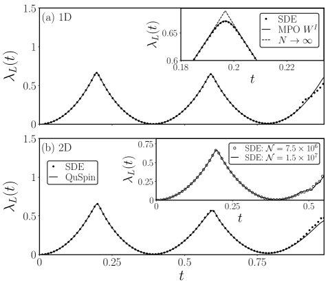
Figure 2: Loschmidt rate function, $\lambda_{L}(t)$, following a quantum quench in the 1D and 2D quantum Ising model. We start in the ground state $\lvert\psi(0)\rangle=\frac{1}{\sqrt{2}}(\lvert\Downarrow\rangle+\lvert\Uparrow\rangle)$ for $\Gamma=0$ and quench to $\Gamma=8J$. (a) 1D case with $N=50$ spins. The results obtained from the SDEs (dots) are in excellent agreement with those obtained via the MPO $W^{I}$ method (solid line). Deviations occur for $t\gtrsim 1/J$ as the stochastic fluctuations become harder to sample. The inset shows a zoomed in portion of the first Loschmidt peak for $N=75$ spins, demonstrating similar agreement with MPO $W^{I}$. For comparison, we show the exact results of Heyl et al. Heyl et al. (2013) in the thermodynamic limit (dashed line). It is readily seen that the rounding of the Loschmidt peak is a finite-size effect. In both figures we use a time-step of $dt=10^{-2}$, except in the vicinity of the peaks, where $dt=10^{-3}$ is used. The results are obtained by averaging over $10^{7}$ stochastic samples. (b) 2D case for a $5\times 5$ lattice using $1.5\times 10^{7}$ samples. The results are in agreement with QuSpin Weinberg and Bukov (2019) (solid line). The inset shows results for a $7\times 7$ lattice, which cannot be obtained using QuSpin. Convergence is checked by changing the number of samples.

Loschmidt Amplitude.— As discussed in De Nicola et al. (2019); De Nicola et al. , one of the simplest quantities to examine in the stochastic approach is the Loschmidt amplitude, $A(t)\equiv\langle\psi(0)\rvert\hat{U}(t)\lvert\psi(0)\rangle$. The corresponding rate function $\lambda_{L}(t)\equiv-\frac{1}{N}\ln|A(t)|^{2}$ plays a similar role to the equilibrium free energy density: as $N\rightarrow\infty$ it exhibits non-analytic peaks at DQPTs Heyl et al. (2013). We first consider the one-dimensional case. In order to compare to results obtained in the thermodynamic limit Heyl et al. (2013) it is convenient to evolve from the ground state $\lvert\psi(0)\rangle=\frac{1}{\sqrt{2}}(\lvert\Downarrow\rangle+\lvert\Uparrow\rangle)$ at $\Gamma=0$. Here $\lvert\Uparrow\rangle$ and $\lvert\Downarrow\rangle$ correspond to the states with all the spins pointing up and down respectively. Time-evolving these separately using the SDEs (5) one obtains:

$$A(t) =\frac{1}{\sqrt{2}}\left(\langle\psi(0)\rvert\hat{U}^{s}(t)\lvert\Downarrow\rangle_{\phi}+\langle\psi(0)\rvert\hat{U}^{s}(t)\lvert\Uparrow\rangle_{\phi}\right),$$ (9)

where $\langle\psi(0)\rvert\hat{U}^{s}(t)\lvert\Downarrow\rangle=\frac{1}{\sqrt{2}}\prod_{j}(1+\xi^{+}_{j}(t))e^{\frac{-\xi^{z}_{j}(t)}{2}},$ and $\langle\psi(0)\rvert\hat{U}^{s}(t)\lvert\Uparrow\rangle$ is obtained by $\xi^{a}\rightarrow{\bar{\xi}}^{a}$. The SDEs are solved with the initial conditions $\xi^{a}(0)=0$ and $\bar{\xi}^{a}(0)=0$ respectively. The results for $\lambda_{L}(t)$ corresponding to time-evolution with $\Gamma=8J$ are shown in Fig. 2(a), for a 1D system with $N=50$ spins. The results go beyond what is achievable using Exact Diagonalization (ED) and are in excellent agreement with those obtained via the MPO $W^{I}$ method Zaletel et al. (2015), implemented using ITensor ITE . Deviations are observed for $t\gtrsim 1/J$ as the stochastic fluctuations become harder to sample. The inset shows the first Loschmidt peak for $N=75$, which again demonstrates excellent agreement. For comparison we display exact results obtained in the thermodynamic limit, $N\rightarrow\infty$ Heyl et al. (2013). Although the finite-size effects are stronger in the vicinity of the peak, the SDE and MPO results remain coincident for all of the system sizes considered. Results for the same quench on a $5\times 5$ lattice in 2D are shown in Fig. 2(b) (dots), and are verified against those obtained using QuSpin’s time-evolution solver Weinberg and Bukov (2019) (solid line). The inset shows the first Loschmidt peak for a $7\times 7$ lattice, which goes beyond what we can readily verify using other techniques. We check for convergence near the peak by doubling the number of samples, $\mathcal{N}$, and noting that the results change by less than $0.5\%$ in this region.

Growth of Fluctuations.— To quantify the role of stochastic fluctuations it is instructive to consider the spectrum of an effective Hamiltonian, $\hat{H}_{\text{eff}}(t)$, defined by

$$\hat{U}^{s}(t)=\prod_{j}e^{\xi^{+}_{j}(t)\hat{S}^{+}_{j}}e^{\xi^{z}_{j}(t)\hat{S}^{z}_{j}}e^{\xi^{-}_{j}(t)\hat{S}^{-}_{j}}\equiv e^{-i\hat{H}_{\text{eff}}t},$$ (10)

in analogy to Floquet systems Rahav et al. (2003). Since $\hat{U}^{s}(t)$ is non-unitary, the eigenvalues of $\hat{H}_{\text{eff}}$, $\varepsilon=\varepsilon_{R}+i\varepsilon_{I}$, are generically complex. The spectrum of $\hat{H}_{\text{eff}}(t)$ can be calculated directly from (10) by time-evolving the SDEs to the time of interest. This can also be obtained by noting that $\hat{U}^{s}(t)$ can be calculated directly as a product of random matrices, $\hat{U}^{s}(t)=\hat{U}^{s}(t,t-\delta)\hat{U}^{s}(t-\delta,t-2\delta)...\hat{U}^{s}(\delta,0)$, by time-slicing into small intervals of size $\delta$, without the disentangling transformation. In Fig. 3 we show the time-evolution of the eigenvalue distribution of $\hat{H}_{\rm eff}$, for $100$ stochastic samples with $\Gamma=8J$ and $N=10$ in 1D. It can be seen that the distribution of $\varepsilon_{R}$ is uniform at late times, whilst that of $\varepsilon_{I}$ is well approximated by a normal distribution. In the Supplementary Material we show that the variance of the distribution of $\varepsilon_{I}$, denoted by $\sigma^{2}(t)=\langle\varepsilon_{I}^{2}\rangle-\langle\varepsilon_{I}\rangle^{2}$, exhibits damped oscillations as a function of time, with extrema that occur in proximity to those in the time-dependent magnetization. In general, the presence of the positive imaginary eigenvalues results in the growth of the norm of individual stochastic states over time. Due to the effect of finite numerical sampling, this leads to the growth of the norm of the overall quantum state, and to departures for physical observables. As we will see below, this can be partially compensated by rescaling by the norm.

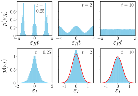
Figure 3: Normalized eigenvalue distributions of the effective Hamiltonian $\hat{H}_{\text{eff}}$ for the 1D quantum Ising model with $\Gamma=8J$ and $N=10$, obtained via the SDEs with $dt=10^{-4}$. The upper and lower panels show the real and imaginary parts, $\varepsilon_{R}$ and $\varepsilon_{I}$ respectively, at times $t=0.25,2,10$; the abscissa in the upper plots is scaled by time. The results correspond to a small number of samples, $\mathcal{N}=100$, to illustrate the non-Hermitian character of the stochastic representation. The distribution of $\varepsilon_{R}$ is approximately uniform at late times whereas the distribution of $\varepsilon_{I}$ is approximately normal, as shown by the solid (red) lines.

Magnetization Dynamics.— As discussed in De Nicola et al. (2019); De Nicola et al. , time-dependent physical observables can be obtained by using two Hubbard–Stratonovich transformations to decouple the forwards and backwards evolution operators:

$$\langle\hat{O}(t)\rangle=\langle\psi(0)\rvert\hat{U}^{s\dagger}(\tilde{\phi})\hat{O}\hat{U}^{s}(\phi)\lvert\psi(0)\rangle_{\phi,\tilde{\phi}},$$ (11)

where $\phi$ and $\tilde{\phi}$ are independent noise variables. In this representation, the local magnetization is given by De Nicola et al. (2019)

$$\langle\hat{S}^{z}_{j}\rangle=-\frac{1}{2}\Big{\langle}e^{-\frac{1}{2}(\chi^{z}+\tilde{\chi}^{z*})}\Big{(}1-\xi^{+}_{j}\tilde{\xi}^{+*}_{j}\Big{)}\prod_{i\neq{j}}\Big{(}1+\xi^{+}_{i}\tilde{\xi}^{+*}_{i}\Big{)}\Big{\rangle}_{\phi,\tilde{\phi}},$$ (12)

where $\chi\equiv\sum_{i}\xi^{z}_{i}$, $\tilde{\chi}\equiv\sum_{i}\tilde{\xi}^{z}_{i}$, and we implicitly take the real part; in general, observables have imaginary parts which vanish in the limit of infinite sampling Drummond and Gardiner (1980); Barry and Drummond (2008); Ng et al. (2013). In Fig. 4(a) we show results for the time-dependent magnetization $\mathcal{M}(t)=\frac{1}{N}\sum_{j}\langle\hat{S}^{z}_{j}(t)\rangle,$ following a quantum quench from the fully-polarized initial state $\lvert\Downarrow\rangle$ to $\Gamma=8J$ for a 1D system with $N=25$ spins. The results are in good agreement with MPO calculations until times $t\gtrsim 1/J$ when stochastic fluctuations become large. In Fig. 4(b) we show results for the norm of the time-evolving state as computed from the SDEs:

$$|\psi(t)|^{2}=\Big{\langle}e^{-\frac{1}{2}(\chi^{z}+\tilde{\chi}^{z*})}\prod_{i}\Big{(}1+\xi^{+}_{i}\tilde{\xi}^{+*}_{i}\Big{)}\Big{\rangle}_{\phi,\tilde{\phi}},$$ (13)

where again, we take the real part. It is readily seen that the norm departs from unity once the stochastic fluctuations become significant. In Fig. 4(c) we show results for the re-scaled magnetization $\mathcal{M}_{res}(t)={\mathcal{M}}(t)/|\psi(t)|^{2}$ which provides much better agreement with the MPO results until later times. Fluctuations in $\mathcal{M}_{res}(t)$ still occur however, especially when the norm of the state is close to zero. This clearly highlights the importance of normalization and stochastic sampling in the computation of observables.

Matrix Product States.— Another approach to reducing fluctuations in observables is to decompose the time-evolving state into a matrix product state (MPS):

$$\lvert\psi(t)\rangle=\sum_{\begin{subarray}{c}\sigma_{1},..\sigma_{n}\\ d_{1},..d_{n-1}\end{subarray}}A_{1,d_{1}}^{\sigma_{1}}A_{d_{1},d_{2}}^{\sigma_{2}}....A_{d_{n-1},1}^{\sigma_{n}}\lvert\sigma_{1}\sigma_{2}...\sigma_{n}\rangle,$$ (14)

where $\mathbf{A}^{\sigma_{i}}$ are matrices with physical spin indices, $\sigma_{i}$, and auxiliary indices $d_{i}\in 1,\dots,D_{i}$, where $D_{i}$ are the bond dimensions; see Schollwöck (2011) for an introduction. This reduces the number of noise variables required since only a single Hubbard–Stratonovich transformation is needed for time-evolution; see Supplementary Material. One may also calculate the norm of the state using MPS techniques, thereby eliminating fluctuations from the stochastic sampling of $|\psi(t)|^{2}$. In Fig 4(d) we show the results of the hybrid stochastic-MPS approach for a quantum quench in a 1D system with $N=50$ spins. The results are in excellent agreement with the MPO approach, in spite of doubling the system size and reducing the number of stochastic samples. A notable disadvantage of this hybrid approach is that one must store the MPS state in memory at the expense of the stochastic parallelization. Nonetheless, the marriage of these approaches may be useful for future developments.

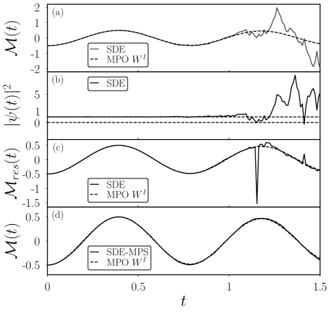
Figure 4: (a) Time-dependent magnetization $\mathcal{M}(t)$ following a quantum quench in the 1D quantum Ising model from the fully-polarized initial state $\lvert\Downarrow\rangle$ to $\Gamma=8J$ with $N=25$ spins. The results obtained from the SDEs (solid line) with $2.5\times 10^{6}$ samples are in agreement with MPO $W^{I}$ (dashed line) until $t\sim 1/J$. (b) Time-evolution of the norm of the quantum state $|\psi(t)|^{2}$ following the quench in (a). The norm departs from unity when the stochastic fluctuations become significant. (c) Time-evolution of the rescaled magnetization $\mathcal{M}_{res}(t)$ showing better agreement with MPO $W^{I}$. It can be seen that fluctuations in $\mathcal{M}_{res}(t)$ occur whenever $|\psi(t)|^{2}$ is close to zero. (d) Time-evolution of ${\mathcal{M}}(t)$ using a hybrid stochastic-MPS approach for $N=50$ spins, with $50,000$ samples and a maximum bond dimension of $D_{i}=20$. The results are in good agreement with MPO $W^{I}$ (dashed line).

Conclusions.— In this work we have demonstrated that the stochastic approach to non-equilibrium quantum spin systems can address significantly larger systems than recently obtained, in both one and two dimensions. We have shown that the non-Hermitian character of the representation leads to a growth of the norm of $\lvert\psi(t)\rangle$, due to the effect of finite numerical sampling. However, this can be compensated for by rescaling by the norm. We have shown that the approach can be combined with a decomposition in terms of matrix product states, for the calculation of time-dependent observables. There are many directions for research, including extensions to larger system sizes and later times, particularly in higher dimensions where few techniques are available.

Acknowledgements.— We acknowledge helpful conversations with S. De Nicola, B. Doyon, D. O’Dell and S. Wüster. We also thank J. Morley for assistance with the implementation of MPS algorithms. SEB is supported by the EPSRC CDT in Cross-Disciplinary Approaches to Non-Equilibrium Systems (CANES) via grant number EP/L015854/1. We are grateful to the UK Materials and Molecular Modelling Hub for computational resources, which is partially funded by EPSRC (EP/P020194/1). The MPO calculations were performed using the ITensor Library ITE . MJB acknowledges the support of the ICTS (Bengaluru) during the program on Non-Hermitian Physics PHHQP XVIII. AGG acknowledges EPSRC grant EP/P013449/1.

I Supplementary Material

II I. Parametrization

As discussed in the main text, we may eliminate divergent trajectories from the SDEs (5) by a suitable parametrization of the stochastic time-evolution operator, $\hat{U}^{s}_{j}(t)$. Adopting the Gauss parametrization of SL(2,$\mathbb{C}$) Ringel and Gritsev (2013)

$$\hat{U}^{s}_{j}(t)\equiv e^{\xi^{+}_{j}(t)\hat{S}^{+}_{j}}e^{\xi^{z}_{j}(t)\hat{S}^{z}_{j}}e^{\xi^{-}_{j}(t)\hat{S}^{-}_{j}}.$$ (15)

For spin-$1/2$ systems this can be represented in matrix form as

$$\hat{U}^{s}_{j}(t)=\begin{pmatrix}e^{\frac{1}{2}\xi^{z}_{j}}+\xi^{+}_{j}\xi^{-}_{j}e^{-\frac{1}{2}\xi^{z}_{j}}&\xi^{-}_{j}e^{-\frac{1}{2}\xi^{z}_{j}}\\ \xi^{+}_{j}e^{-\frac{1}{2}\xi^{z}_{j}}&e^{-\frac{1}{2}\xi^{z}_{j}}\end{pmatrix},$$ (16)

where $\xi^{\pm,z}_{j}\in\mathbb{C},$ and the initial conditions $\xi^{\pm,z}_{j}(0)=0$ ensure that $\hat{U}^{s}_{j}(0)=\mathbb{1}$ is the identity operator. In general, this corresponds to a representation of the group SL(2,$\mathbb{C}$) with three complex parameters. The action of $\hat{U}^{s}_{j}(t)$ on a generic initial state $\lvert\psi_{j}(0)\rangle=a\lvert\downarrow\rangle+b\lvert\uparrow\rangle$, with $a,b\in\mathbb{C}$ yields

$$\lvert\psi^{s}_{j}(t)\rangle=e^{-\frac{1}{2}\xi^{z}_{j}(t)}\Big{[}\big{(}a+b\xi^{-}_{j}(t)\big{)}\lvert\downarrow\rangle+\big{(}a\xi^{+}_{j}(t)+be^{\xi^{z}_{j}(t)}+b\xi^{+}_{j}(t)\xi^{-}_{j}(t)\big{)}\lvert\uparrow\rangle\Big{]},$$ (17)

Although (17) is formally exact, the parametrization contains some redundancy: an arbitrary un-normalized spin state can be represented by four parameters, including the overall phase. To see that a reduction is possible it is instructive to consider an initial spin-down state $\lvert\downarrow\rangle$ corresponding to $a=1$ and $b=0$. This yields

$$\lvert\psi^{s}_{j}(t)\rangle=\hat{U}^{s}_{j}(t)\lvert\downarrow\rangle=e^{-\frac{1}{2}\xi^{z}_{j}(t)}\big{(}\lvert\downarrow\rangle+\xi^{+}_{j}(t)\lvert\uparrow\rangle\big{)},$$ (18)

where the complex parameter $\xi^{-}_{j}(t)$ has dropped out. In this case, the divergence in the SDE (5a) corresponding to $|\xi_{j}^{+}|\rightarrow\infty$ is associated with an inability to parametrize the spin-up state $\lvert\uparrow\rangle$, using a projective representation of the Bloch sphere. As discussed in the main text and in Section II below, this can be avoided by using a two-patch parametrization. Although these considerations apply only for an initially spin-down state, more general initial states can always be prepared by rotation from this state. Explicitly, we may introduce a state-preparation protocol starting at $t=-\delta$, with $\delta>0$, and evolving deterministically until $t=0$. In this approach, the time-evolution operator takes the form $\hat{U}^{s}_{j}(t,-\delta)=\mathbb{T}e^{-i\int_{-\delta}^{t}\hat{H}^{s}_{j}(t^{\prime})dt^{\prime}}$ where

$$\hat{H}^{s}_{j}(t)=\begin{cases}\alpha_{j}^{a}\hat{S}^{a}_{j},~{}~{}~{}~{}~{}~{}-\delta\leq t<0;\\ \Phi^{a}_{j}(t^{\prime})\hat{S}^{a}_{j},~{}~{}~{}~{}~{}~{}~{}~{}~{}~{}t\geq 0,\end{cases}$$ (19)

and the coefficients $\alpha_{j}^{a}$ specify the initial conditions according to $\lvert\psi^{s}_{j}(0)\rangle=\hat{U}^{s}_{j}(0,-\delta)\lvert\downarrow\rangle$. In practice, this is equivalent to setting non-trivial initial conditions for the $\xi$-variables and evolving under the SDEs (5). For example, the initial state $\lvert\psi_{j}(0)\rangle=\frac{1}{\sqrt{2}}\big{(}\lvert\downarrow\rangle+\lvert\uparrow\rangle\big{)}$ corresponds to $\xi^{+}_{j}(0)=1$ and $\xi^{z}_{j}(0)=\ln 2,$ as follows directly from (18). In this approach the trivial initial conditions correspond to $t=-\delta$, so that $\xi_{j}^{+}(-\delta)=\xi_{j}^{-}(-\delta)=\xi_{j}^{z}(-\delta)=0$ and $\hat{U}^{s}_{j}(-\delta,-\delta)=\mathbb{1}$.

In general, the time-evolution of an arbitrary product state is given by

$$\lvert\psi(t)\rangle=\Big{\langle}\prod_{j}e^{-\frac{1}{2}\xi^{z}_{j}(t)}\big{(}\lvert\downarrow\rangle+\xi^{+}_{j}(t)\lvert\uparrow\rangle\big{)}\Big{\rangle}_{\phi},$$ (20)

where the initial conditions $\xi^{a}_{j}(0)$ specify the initial spin-orientation at each site. A generic superposition can be obtained by summing over (20) with the appropriate initial conditions. Stochastic expressions for physical observables are readily obtained from the projective representation (18). For example, the Loschmidt amplitude to remain in the spin-down state is given by $A(t)=\langle e^{-\frac{1}{2}\sum_{j}\xi_{j}^{z}(t)}\rangle_{\phi}$, in agreement with (9) and De Nicola et al. (2019). In a similar way, the quantum expectation value of the spin operator $\hat{\mathbf{S}}_{j}$ is given by

$$\langle\hat{\mathbf{S}}_{j}(t)\rangle=\Big{\langle}\prod_{i}|\psi_{i}^{s}(t)|^{2}\mathbf{n}_{j}(t)\Big{\rangle}_{\phi,\tilde{\phi}},$$ (21)

where

$$\mathbf{n}_{j}(t)=\frac{1}{2}\Bigg{(}\frac{2\text{Re}(\xi^{+}_{j}(t))}{1+|\xi^{+}_{j}(t)|^{2}},\frac{-2\text{Im}(\xi^{+}_{j}(t))}{1+|\xi^{+}_{j}(t)|^{2}},\frac{-1+|\xi^{+}_{j}(t)|^{2}}{1+|\xi^{+}_{j}(t)|^{2}}\Bigg{)}$$ (22)

corresponds to the position of a spin on the Bloch sphere. The factor of

$$|\psi_{i}^{s}(t)|^{2}=e^{-\text{Re}(\xi^{z}_{i}(t))}(1+|\xi^{+}_{i}(t)|^{2})$$ (23)

is the norm of the state $\lvert\psi_{i}^{s}(t)\rangle$. In writing (21), (22) and (23), it is implicit that $\xi^{a*}_{j}$ is an independent variable from $\xi^{a}_{j}$, which we denote by $\tilde{\xi}^{a*}_{j}=\xi^{a*}_{j}$ in the main text. The result (21) is readily generalized to multipoint correlation functions. For example,

$$\langle\hat{S}^{a}_{j}(t)\hat{S}^{b}_{k}(t)\rangle=\Big{\langle}\prod_{i}|\psi_{i}^{s}(t)|^{2}n_{j}^{a}(t)n_{k}^{b}(t)\Big{\rangle}_{\phi,\tilde{\phi}}.$$ (24)

The expressions for entangled states can be obtained by averaging over the initial conditions for $\xi(0)$ and $\tilde{\xi}(0)$.

III II. Eliminating divergent trajectories

As discussed above and in the main text, the SDE (5a) exhibits divergences corresponding to $|\xi^{+}_{j}|\rightarrow\infty$. These can be avoided by two-patch parametrization of the Bloch sphere. To this end, it is convenient to define new variables $\bar{\xi}^{a}$ via the generalization of equation (18), where the roles of $\lvert\downarrow\rangle$ and $\lvert\uparrow\rangle$ are interchanged:

$$\lvert\psi^{s}_{j}(t)\rangle=\Big{(}\bar{\xi}^{+}_{j}(t)\lvert\downarrow\rangle+\lvert\uparrow\rangle\Big{)}e^{-\frac{1}{2}\bar{\xi}^{z}_{j}(t)}.$$ (25)

Equating the coefficients of (18) and (25), one obtains the identifications

$$\bar{\xi}^{+}_{j}(t)=\frac{1}{\xi^{+}_{j}(t)},~{}\bar{\xi}^{z}_{j}(t)=\xi^{z}_{j}(t)-2\ln(\xi^{+}_{j}(t)).$$ (26)

This coordinate system is related to the original Gauss parametrization (15) by swapping the pole of projection from the North to the South pole. Performing this change of variables, the SDEs (5a) and (5b) become

$$i\dot{\bar{\xi}}^{+}_{j}=\Phi^{-}_{j}-\Phi^{z}_{j}\bar{\xi}^{+}_{j}-\Phi^{+}_{j}\bar{\xi}_{j}^{+2},$$ (27a)

$$i\dot{\bar{\xi}}^{z}_{j}=-\Phi^{z}_{j}-2\Phi^{+}_{j}\bar{\xi}^{+}_{j}.$$ (27b)

A convenient place to perform the change of variables (26) is when the spins cross the equator, since the magnitude of $|\xi^{+}_{j}(t)|=|\bar{\xi}^{+}_{j}(t)|=1$ at this point, and the numerical error associated with simulating the nonlinear term in (5a) is minimized. This approach is also used in Ng et al. (2013). In practice, the initial state will determine which parametrization is initialized on each site. Denoting

$$\zeta_{j}^{+}(t)=\begin{cases}\xi^{+}_{j}(t),~{}~{}~{}\text{lower half-sphere with }|\xi_{j}^{+}|\in[0,1];\\ \bar{\xi}^{+}_{j}(t),~{}~{}~{}\text{upper half-sphere with }|\bar{\xi}_{j}^{+}|\in[0,1),\end{cases}$$ (28)

one may track the dynamics of this single variable over all times. In Fig. 5 we plot the time-evolution of the single-patch variable $|\xi_{1}^{+}(t)|$ following a quantum quench in the 1D quantum Ising model. For the chosen parameters and the specific noise realization, it can be seen that this quantity diverges at time $t_{div}=6.25$. As a result, $\dot{\xi}_{1}^{+}(t)$ overflows due to the $\xi_{1}^{+^{2}}(t)$ term in (5a), and numerical integration fails for this trajectory. In contrast, the two-patch variable $|\zeta^{+}_{1}(t)|$ remains finite, and we can evolve beyond $t_{div}$. This enables us to retain all the stochastic trajectories when computing the time-dependent magnetization, in contrast to previous work De Nicola et al. (2019); De Nicola et al. .

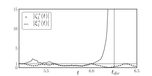
Figure 5: Time-evolution of a divergent trajectory $|\xi^{+}_{1}(t)|$ (solid line) following a quantum quench in the 1D quantum Ising model from the fully polarized state $\lvert\Downarrow\rangle$ to $\Gamma=8J$, with $N=7$ spins. The diverging quantity is evaluated on the first site, and overflows at $t_{div}=6.25$. For comparison, the two-patch variable $|\zeta^{+}_{1}(t)|$ (dotted) does not diverge.

To analyze the spectrum of $\hat{U}^{s}(t,0)$, or equivalently $\hat{H}_{\text{eff}}=\frac{i}{t}\ln\hat{U}^{s}(t,0)$ as illustrated in Fig. 3, the parameter $\xi^{-}_{j}$ is also required; this dropped out in (18). Under the transformation $(\xi^{+}_{j},\xi^{z}_{j})\rightarrow(\bar{\xi}^{+}_{j},\bar{\xi}^{z}_{j})$ the SDE (5c) becomes

$$i\dot{\xi}^{-}_{j}=\Phi^{-}_{j}\frac{e^{\bar{\xi}^{z}_{j}}}{\bar{\xi}^{+2}}.$$ (29)

In order to ensure that (29) is well-behaved as $\bar{\xi}^{+}_{j}\rightarrow 0$ it is convenient to make the change of variables

$$\xi_{j}^{-}\rightarrow\bar{\xi}^{-}_{j}\equiv\xi^{-}_{j}+\frac{e^{\bar{\xi}^{z}_{j}}}{\bar{\xi}^{+}_{j}}.$$ (30)

The resulting SDE for $\bar{\xi}^{-}_{j}$ is given by

$$i\dot{\bar{\xi}}^{-}_{j}=-\Phi^{+}_{j}e^{\bar{\xi}^{z}_{j}},$$ (31)

which mirrors (5c) up to a sign change and $\Phi^{-}_{j}\rightarrow\Phi^{+}_{j}$. The maps (26) and (30) can now be conducted simultaneously to avoid the divergence associated with $\xi^{+}_{j}\rightarrow\infty$, allowing $\hat{U}^{s}(t,0)$ to be calculated at much later times. Eventually this strategy will break down if (5c) or (31) cannot be integrated due to $e^{\xi^{z}_{j}}\rightarrow\infty$ or $e^{\bar{\xi}^{z}_{j}}\rightarrow\infty$ respectively. However, $\xi^{-}_{j}$ and $\bar{\xi}^{-}_{j}$ are not required for the time-dependent magnetization, this is not a limitation. The spectrum of $\hat{H}_{\text{eff}}$ (10) is calculated directly from trajectories by mapping between the $\xi^{a}_{j}$ and $\bar{\xi}^{a}_{j}$ variables in accordance with the prescription (28). As discussed in the main text, damped oscillations of the variance of the imaginary eigenvalues of $\hat{H}_{\text{eff}}$ occur as a function of time; see Fig. 6.

IV III. Hybrid technique with matrix product states

As discussed in the main text, the time-evolving quantum state evaluated within the stochastic approach can be represented as a matrix product state. This halves the number of noise variables required since only a single Hubbard–Stratonovich transformation is needed to evaluate $\lvert\psi(t)\rangle=\hat{U}(t)\lvert\psi(0)\rangle$. However, this comes at the cost of storing the state in memory, so the method is no longer fully parallelizable. Here we demonstrate how this representation is obtained. The quantum state is first written as the sample average of the stochastic state:

$$\lvert\psi(t)\rangle=\lvert\psi^{s}(t)\rangle_{\phi}=\frac{1}{\mathcal{N}}\sum_{r=1}^{\mathcal{N}}\prod_{i}^{N}\Big{(}\lvert\downarrow\rangle+\xi^{+,r}_{i}\lvert\uparrow\rangle\Big{)}e^{-\frac{\xi^{z,r}_{i}}{2}},$$ (32)

where $r=1,...,\mathcal{N}$ is the sample index. A matrix product state (MPS) is given by

$$\lvert\psi\rangle=\sum_{\begin{subarray}{c}\sigma_{1},..,\sigma_{N}\\ d_{1},..,d_{N-1}\end{subarray}}A_{1,d_{1}}^{\sigma_{1}}A_{d_{1},d_{2}}^{\sigma_{2}}....A_{d_{N-1},1}^{\sigma_{N}}\lvert\sigma_{1}\sigma_{2}...\sigma_{N}\rangle,$$ (33)

where the matrices $\mathbf{A}^{\sigma_{i}}$ carry physical spin indices $\sigma_{i}$ and auxiliary indices $d_{i}\in 1,...,D_{i}$, where $D_{i}$ are the bond dimensions. To cast the state (32) into MPS form, we first note that each configuration of indices $d_{1},d_{2},…$ in (33) forms a product state that can be identified as one term in the sum (32). We can identify a trivial, inefficient MPS representation of (32) by taking a diagonal form for the MPS tensors. For example

$$\mathbf{A}^{\downarrow}=\begin{pmatrix}e^{-\frac{\xi^{z,1}_{i}}{2}}&0&....&0\\ 0&e^{-\frac{\xi^{z,2}_{i}}{2}}&...&0\\ \vdots&\vdots&\ddots&\vdots\\ 0&0&...&e^{-\frac{\xi^{z,\mathcal{N}}_{i}}{2}}\\ \end{pmatrix},$$ (34)

where the factor of $1/\mathcal{N}$ in (32) can be absorbed into one of the $\mathbf{A}^{\sigma_{i}}$ matrices. The state $\lvert\psi\rangle$ can be compressed to a lower bond-order, full rank MPS by using a sequence of singular value decompositions (SVDs). In practice, we may perform this procedure in batches. The MPS tensors in each batch can be further combined and compressed by first collecting them into a block diagonal MPS tensor given by

$$\mathbf{A}^{\sigma_{i}}=\begin{pmatrix}\mathbf{A}^{\sigma_{i},1}&0&....&0\\ 0&\mathbf{A}^{\sigma_{i},2}&...&0\\ \vdots&\vdots&\ddots&\vdots\\ 0&0&...&\mathbf{A}^{\sigma_{i},k}\\ \end{pmatrix},$$ (35)

where the batch index runs from 1 to $k$. A subsequent sequence of SVDs would again lead to an MPS with reduced bond order and full rank. For example, the results in Fig. 4 were obtained by dividing the $50,000$ trajectories into 50 batches of size 1000. After the initial compression, the batches were combined in pairs according to (35) and compressed again. This was repeated two more times in groups of five batches. In practice, if the bond dimension after a compression exceeds the nominal value of 20 we truncate it back to this value. Since the mapping to MPS must be carried out at each time where observables are calculated, it is more efficient to only carry it out at the times of interest.

For all the MPO $W^{I}$ Zaletel et al. (2015) simulations carried out in the main text we use a maximum bond dimension of $50$, a minimum singular value cut-off of $10^{-14}$, and a time-step of $dt=0.001$.

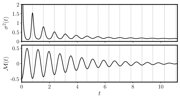
Figure 6: Normalized eigenvalue distributions of the effective Hamiltonian $\hat{H}_{\text{eff}}$ for the 1D quantum Ising model with $\Gamma=8J$ and $N=10$. The variance, $\sigma^{2}(t)$, of the distribution of $\varepsilon_{I}$ exhibits damped oscillations as a function of time. The extrema occur in proximity to the turning points in the magnetization, $\mathcal{M}(t)$, obtained via exact diagonalization, following a quench from the fully-polarized initial state $\lvert\Downarrow\rangle$ to $\Gamma=8J$ for $N=10$ spins, as indicated by the vertical lines.

V IV. Scaling

In order to quantify the scaling properties of the real-time stochastic approach, we consider the time-scale over which the simulations are accurate as a function of the system size and the number of samples. Since the stochastic approach only produces perfectly normalized quantum states in the limit $\mathcal{N}\rightarrow\infty$, deviations of the norm from unity can provide an estimate of the simulation’s convergence and the time-scale over which the method can be trusted. As illustrated in Fig. 3, rescaling by the norm can lead to good approximations for physical observables, even if the norm deviates significantly from unity. In view of this, we define the breakdown time, $t_{b}$, as the earliest time for which a $10\%$ error is observed in the norm. In Fig. 7(a) we show $t_{b}$ as a function of the inverse system size $N^{-1}$, for quenches in the 1D quantum Ising model from the fully polarized initial state $\lvert\Downarrow\rangle$ to $\Gamma=8J$, for a fixed number of samples $\mathcal{N}=10^{6}$. The data are well approximated by the linear relation

$$Jt_{b}=16.94N^{-1}+0.12.$$ (36)

That is to say, for a fixed number of samples the breakdown time scales with the inverse of the system size. This is consistent with the results of De Nicola et al. . In Fig. 7(b) we also show $t_{b}$ as a function of the number of samples, for the same quench, but for a fixed system size, with $N=7$ spins. The data are compatible with the relation $Jt_{b}=0.22\ln\mathcal{N}-0.6$, i.e. the number of samples required to reach a given time $t_{b}$ therefore scales exponentially, $\mathcal{N}\propto e^{\alpha Jt_{b}}$, where $\alpha\approx 4.5$, in this example. This is consistent with the scaling of fluctuations analyzed in De Nicola et al. using different diagnostics.

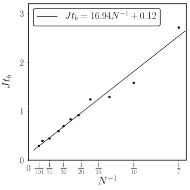
(a)

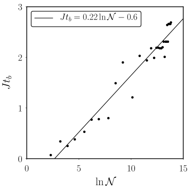
(b)

Figure 7: (a) Breakdown time, $t_{b}$, of the simulations following a quantum quench in the 1D quantum Ising model from the fully polarized initial state $\lvert\Downarrow\rangle$ to $\Gamma=8J$. The breakdown time is defined as the time at which the norm deviates by $10\%$ from unity. (a) Scaling of $t_{b}$ with inverse system size with $\mathcal{N}=10^{6}$ held fixed. The data are well approximated by a linear fit (solid line), particularly for large system sizes. (b) Scaling of $t_{b}$ with the number of samples for a fixed system size with $N=7$. The linear fit (solid line) suggests an exponential dependence of the number of samples on the $t_{b}$ according to $\mathcal{N}\propto e^{\alpha Jt_{b}}$, with $\alpha\approx 4.5$.

References

Friedenauer et al. (2008)A. Friedenauer, H. Schmitz, J. T. Glueckert, D. Porras, and T. Schaetz, Nat.
Phys. 4, 757 (2008).
Simon et al. (2011)J. Simon, W. S. Bakr,
R. Ma, M. E. Tai, P. M. Preiss, and M. Greiner, Nature 472, 307 (2011).
Meinert et al. (2013)F. Meinert, M. J. Mark,
E. Kirilov, K. Lauber, P. Weinmann, A. J. Daley, and H. C. Nägerl, Phys. Rev. Lett. 111, 1
(2013).
Jurcevic et al. (2014)P. Jurcevic, B. P. Lanyon, P. Hauke,
C. Hempel, P. Zoller, R. Blatt, and C. F. Roos, Nature 511, 202 (2014).
Jurcevic et al. (2017)P. Jurcevic, H. Shen,
P. Hauke, C. Maier, T. Brydges, C. Hempel, B. P. Lanyon, M. Heyl, R. Blatt, and C. F. Roos, Phys. Rev. Lett. 119, 1 (2017).
Klimov and Chumakov (2009)A. B. Klimov and S. M. Chumakov, A group-theoretical
approach to quantum optics: models of atom-field interactions (John Wiley & Sons, 2009).
Rümelin (1982)W. Rümelin, SIAM J. Numer. Anal 19, 604 (1982).
Klöden and Platen (1992)P. E. Klöden and E. Platen, Numerical Solution of
Stochastic Differential Equations (Springer, 1992).
Schollwöck (2011)U. Schollwöck, Ann. Phys. (N. Y.) 326, 96 (2011).