Polar decomposition based algorithms on the product of Stiefel manifolds with applications in tensor approximation

Abstract.

In this paper, we propose a general algorithmic framework to solve a class of optimization problems on the product of complex Stiefel manifolds based on the matrix polar decomposition. We establish the weak convergence, global convergence and linear convergence rate of this general algorithmic approach using the Łojasiewicz gradient inequality and the Morse-Bott property. This general algorithm and its convergence results are applied to the simultaneous approximate tensor diagonalization and simultaneous approximate tensor compression, which include as special cases the low rank orthogonal approximation, best rank-1 approximation and low multilinear rank approximation for higher order complex tensors. We also present a symmetric variant of this general algorithm to solve a symmetric variant of this class of optimization models, which essentially optimizes over a single Stiefel manifold. We establish its weak convergence, global convergence and linear convergence rate in a similar way. This symmetric variant and its convergence results are applied to the simultaneous approximate symmetric tensor diagonalization, which includes as special cases the low rank symmetric orthogonal approximation and best symmetric rank-1 approximation for higher order complex symmetric tensors. It turns out that well-known algorithms such as LROAT, S-LROAT, HOPM, S-HOPM are all special cases of this general algorithmic framework and its symmetric variant, and our convergence results subsume the results found in the literature designed for those special cases. All the algorithms and convergence results in this paper also apply to the real case.

1. Introduction

Theory and algorithms for optimization over manifolds have been developed and applied widely because of its practical importance; see [4, 10, 31, 66]. In particular, many different algorithms, including the Newton-type methods [6], trust-region algorithm [2] and alternating direction method of multipliers (ADMM) [44], have been proposed for optimization over a single Stiefel manifold or the product of Stiefel manifolds, which capture the orthogonality type of constraints [4, 25, 38, 62, 72].

1.1. Problem formulation

For a matrix $\boldsymbol{X}\in\mathbb{C}^{n\times r}$, we denote by $\boldsymbol{X}^{{\sf T}}$, $\boldsymbol{X}^{*}$ and $\boldsymbol{X}^{{\sf H}}$ its transpose, conjugate and conjugate transpose, respectively. Let $\text{St}(r,n,\mathbb{C})=\{\boldsymbol{X}\in\mathbb{C}^{n\times r}:\boldsymbol{X}^{{\sf H}}\boldsymbol{X}=\boldsymbol{I}_{r}\}$ be the complex Stiefel manifold with $1\leq r\leq n$. In this paper, we mainly study the optimization problem on the product of complex Stiefel manifolds, which is to maximize a smooth function

$$f:\ \Omega\longrightarrow\mathbb{R}^{+},$$ (1)

where

$$\Omega\stackrel{{\scriptstyle\sf def}}{{=}}\text{St}(r_{1},n_{1},\mathbb{C})\times\text{St}(r_{2},n_{2},\mathbb{C})\times\cdots\times\text{St}(r_{d},n_{d},\mathbb{C})$$ (2)

is the product of $d$ complex Stiefel manifolds ($d>1$). Let

$$\Omega^{(i)}\stackrel{{\scriptstyle\sf def}}{{=}}\text{St}(r_{1},n_{1},\mathbb{C})\times\cdots\times\text{St}(r_{i-1},n_{i-1},\mathbb{C})\times\text{St}(r_{i+1},n_{i+1},\mathbb{C})\times\cdots\times\text{St}(r_{d},n_{d},\mathbb{C})$$

be the product of $d-1$ complex Stiefel manifolds and $\nu^{(i)}\in\Omega^{(i)}$. Let $\boldsymbol{U}\in\text{St}(r_{i},n_{i},\mathbb{C})$. Define

$$h_{(i)}:\ \text{St}(r_{i},n_{i},\mathbb{C}) \longrightarrow\mathbb{R}^{+},$$

$$\boldsymbol{U} \longmapsto f(\nu^{(i)},\boldsymbol{U})\stackrel{{\scriptstyle\sf def}}{{=}}f(\boldsymbol{U}^{(1)},\cdots,\boldsymbol{U}^{(i-1)},\boldsymbol{U},\boldsymbol{U}^{(i+1)},\cdots,\boldsymbol{U}^{(d)}).$$ (3)

For simplicity, we also denote by $h_{(i)}$ the natural extension of itself to $\mathbb{C}^{n_{i}\times r_{i}}$. In this paper, we say that the objective function (1) is block multiconvex [54, 64, 75] if the restricted function $h_{(i)}$ is convex for any fixed $\nu^{(i)}\in\Omega^{(i)}$ and $1\leq i\leq d$.

1.2. Symmetric variant

Let $\omega\stackrel{{\scriptstyle\sf def}}{{=}}(\boldsymbol{U}^{(1)},\boldsymbol{U}^{(2)},\cdots,\boldsymbol{U}^{(d)})\in\Omega$. If $r_{i}=r$ and $n_{i}=n$ for all $1\leq i\leq d$, then $\Omega$ in (2) becomes

$$\Omega_{s}\stackrel{{\scriptstyle\sf def}}{{=}}\text{St}(r,n,\mathbb{C})\times\text{St}(r,n,\mathbb{C})\times\cdots\times\text{St}(r,n,\mathbb{C}).$$ (4)

Assume that the objective function $f$ is symmetric on $\Omega_{s}$, that is, $f(\omega)=f(\pi(\omega))$ for any $\omega\in\Omega_{s}$ and permutation $\pi$. In this paper, we also study the symmetric variant of model (1), which is to maximize the smooth function

$$g:\ \text{St}(r,n,\mathbb{C})\longrightarrow\mathbb{R}^{+},\ \boldsymbol{U}\longmapsto f(\boldsymbol{U},\boldsymbol{U},\cdots,\boldsymbol{U}).$$ (5)

For simplicity, we also denote by $g$ the natural extension of itself to $(\mathbb{C}^{n\times r})^{d}$.

1.3. Notations

Let $\mathbb{C}^{n_{1}\times n_{2}\times\cdots\times n_{d}}\stackrel{{\scriptstyle\sf def}}{{=}}\mathbb{C}^{n_{1}}\otimes\mathbb{C}^{n_{2}}\otimes\cdots\otimes\mathbb{C}^{n_{d}}$ be the linear space of $d$-th order complex tensors. Let $\text{symm}(\mathbb{C}^{n\times n\times\cdots\times n})$ be the set of symmetric ones in $\mathbb{C}^{n\times n\times\cdots\times n}$, whose entries do not change under any permutation of indices [20, 60]. For a tensor $\boldsymbol{\mathcal{A}}\in\mathbb{C}^{n_{1}\times n_{2}\times\cdots\times n_{d}}$ and a matrix $\boldsymbol{X}\in\mathbb{C}^{m\times n_{i}}$, we adopt the $i$-mode product defined as $(\boldsymbol{\mathcal{A}}\mathop{\bullet_{i}}\boldsymbol{X})_{p_{1}\cdots q\cdots p_{d}}\stackrel{{\scriptstyle\sf def}}{{=}}\sum_{p_{i}}\mathcal{A}_{p_{1}\cdots p_{i}\cdots p_{d}}X_{qp_{i}}.$ The $i$-mode unfolding of $\boldsymbol{\mathcal{A}}$ is denoted by $\boldsymbol{\mathcal{A}}_{(i)}$, which is the matrix obtained by reordering the $i$-mode fibers of $\boldsymbol{\mathcal{A}}$ in a fixed way [42]. The diagonal of a tensor $\boldsymbol{\mathcal{A}}\in\mathbb{C}^{n_{1}\times n_{2}\times\cdots\times n_{d}}$ is defined as $\mathop{\operator@font diag}\{\boldsymbol{\mathcal{A}}\}\stackrel{{\scriptstyle\sf def}}{{=}}(\mathcal{A}_{11\cdots 1},\cdots,\mathcal{A}_{nn\cdots n})^{{\sf T}}$, where $n=\min(n_{1},\cdots,n_{d})$. We say that $\boldsymbol{\mathcal{A}}$ is diagonal, if its diagonal elements are the only nonzero elements. Let $\boldsymbol{I}_{n\times r}$ be the diagonal matrix in $\mathbb{R}^{n\times r}$ satisfying that the diagonal elements are all equal to 1. Let $\boldsymbol{I}^{\perp}_{n\times r}$ be the matrix in $\mathbb{R}^{n\times(n-r)}$ such that $[\boldsymbol{I}_{n\times r}\ \boldsymbol{I}^{\perp}_{n\times r}]=\boldsymbol{I}_{n}$. We denote by $\|\cdot\|$ the Frobenius norm of a tensor or matrix, or the Euclidean norm of a vector. Let $\mathbb{S}_{n-1}\subseteq\mathbb{C}^{n}$ be the unit sphere, and denote $\mathbb{S}=\mathbb{S}_{0}$ for simplicity. Let $\mathscr{U}_{n}=\text{St}(n,n,\mathbb{C})$ be the unitary group. We denote by $\boldsymbol{e}_{p}$ the $p$-th standard unit vector, and its dimension depends on the context.

1.4. Objective functions of interest

Let $\{\boldsymbol{\mathcal{A}}^{(\ell)}\}_{1\leq\ell\leq L}\subseteq\mathbb{C}^{n_{1}\times n_{2}\times\cdots n_{d}}$ be a set of complex tensors, and $\{\boldsymbol{\mathcal{S}}^{(\ell)}\}_{1\leq\ell\leq L}\subseteq\text{symm}(\mathbb{C}^{n\times n\times\cdots\times n})$ be a set of $d$-th order complex symmetric tensors. Let $\alpha_{\ell}\in\mathbb{R}^{+}$ for $1\leq\ell\leq L$. Denote $(\cdot)^{\dagger}=(\cdot)^{{\sf H}}$ or $(\cdot)^{{\sf T}}$. In this paper, we mainly focus on the following three tensor related objective functions:

• Simultaneous approximate tensor diagonalization:

  $$f(\omega) =\sum\limits_{\ell=1}^{L}\alpha_{\ell}\|\mathop{\operator@font diag}\{\boldsymbol{\mathcal{W}}^{(\ell)}\}\|^{2},\ \ \boldsymbol{U}^{(i)}\in\text{St}(r,n_{i},\mathbb{C}),\ \ 1\leq r\leq n_{i},\ 1\leq i\leq d,$$ (6)

  $$\boldsymbol{\mathcal{W}}^{(\ell)} =\boldsymbol{\mathcal{A}}^{(\ell)}\mathop{\bullet_{1}}(\boldsymbol{U}^{(1)})^{\dagger}\cdots\mathop{\bullet_{d}}(\boldsymbol{U}^{(d)})^{\dagger},\ 1\leq\ell\leq L;$$

• Simultaneous approximate symmetric tensor diagonalization:

  $$g(\boldsymbol{U}) =\sum\limits_{\ell=1}^{L}\alpha_{\ell}\|\mathop{\operator@font diag}\{\boldsymbol{\mathcal{W}}^{(\ell)}\}\|^{2},\ \ \boldsymbol{U}\in\text{St}(r,n,\mathbb{C}),\ \ 1\leq r\leq n,$$ (7)

  $$\boldsymbol{\mathcal{W}}^{(\ell)} =\boldsymbol{\mathcal{S}}^{(\ell)}\mathop{\bullet_{1}}\boldsymbol{U}^{\dagger}\cdots\mathop{\bullet_{d}}\boldsymbol{U}^{\dagger},\ 1\leq\ell\leq L;$$

• Simultaneous approximate tensor compression:

  $$f(\omega) =\sum\limits_{\ell=1}^{L}\alpha_{\ell}\|\boldsymbol{\mathcal{W}}^{(\ell)}\|^{2},\ \ \boldsymbol{U}^{(i)}\in\text{St}(r_{i},n_{i},\mathbb{C}),\ \ 1\leq r_{i}\leq n_{i},\ 1\leq i\leq d,$$ (8)

  $$\boldsymbol{\mathcal{W}}^{(\ell)} =\boldsymbol{\mathcal{A}}^{(\ell)}\mathop{\bullet_{1}}(\boldsymbol{U}^{(1)})^{\dagger}\cdots\mathop{\bullet_{d}}(\boldsymbol{U}^{(d)})^{\dagger},\ 1\leq\ell\leq L.$$

It can be seen that objective functions (6) and (8) are both of form (1), and objective function (7) is the symmetric variant of (6). It will be shown in Section 5.1 and Section 7.1 that objective functions (6) and (8) are both block multiconvex, and in Example 6.9 that the objective function (7) is convex in many cases.

1.5. Tensor approximations

The above three objective functions include the following well-known approximation problems for higher order complex tensors [15, 19, 42, 65] as special cases:

• the objective function (6):

  • the low rank orthogonal approximation [14, 41]: $L=1$;

  • the best rank-1 approximation [22, 24]: $L=1$, $r=1$;

• the objective function (7):

  • the low rank symmetric orthogonal approximation [14, 58, 50]: $L=1$.

  • the best symmetric rank-1 approximation [24, 40]: $L=1$, $r=1$;

• the objective function (8):

  • the low multilinear rank approximation [22, 24]: $L=1$.

  • the best rank-1 approximation [22, 24]: $L=1$, $r_{i}=1$ $(1\leq i\leq d)$.

We seperately consider the best rank-1 approximation and best symmetric rank-1 approximation here (also in Section 5.5 and Section 6.5), because of their own interest and importance, although they are also special cases of the low rank orthogonal approximation, low multilinear rank approximation and their symmetric variants, respectively.

These approximations have been widely used in various fields, including signal processing [19, 21, 30, 39, 53], numerical linear algebra [60, 61] and data analysis [7, 15, 42, 65]. In particular, the best symmetric rank-1 approximation of a real symmetric tensor is corresponding to finding the largest Z-eigenvalue [61]. The low multilinear rank approximation is equivalent to the well-known Tucker decomposition [24, 42], which has been a popular method for data reduction in signal processing and machine learning. When the rank is equal to the dimension (i.e., $r=n$), problem (7) boils down to the simultaneous approximate symmetric tensor diagonalization [18, 49, 51, 52, 70] of complex symmetric tensors by unitary transformations, which is central in Independent Component Analysis (ICA) [16, 17, 22]. Therefore, it is desirable to develop a general algorithmic scheme to solve model (1) and its symmetric variant (5).

1.6. Block coordinate descent

In the literature, the following general block optimization model has been well studied, which is to maximize a smooth function

$$f:\ \mathcal{X}_{1}\times\mathcal{X}_{2}\times\cdots\times\mathcal{X}_{d}\longrightarrow\mathbb{R}^{+},$$ (9)

where $\mathcal{X}_{i}\subseteq\mathbb{R}^{n_{i}}$ is a closed set for $1\leq i\leq d$. A popular approach to solve model (9) is known as block coordinate descent (BCD) [8], with different ways to choose blocks for optimization. One natural choice is the cyclic rule [67, 73], which is also known as the block nonlinear Gauss–Seidel method. In this cyclic approach, the regularized optimization of block multiconvex function was studied in [75], with three different update schemes. Along a similar line, the so-called maximum block improvement (MBI) method was proposed in [13, 54] to optimize the objective function (9), which updates the block of variables corresponding to the maximally improving block at each iteration. Although MBI is more expensive than other methods, it was proved to have better theoretical convergence properties.

1.7. Contributions

In this paper, we mainly develop a general algorithmic scheme to solve model (1) and its symmetric variant (5) based on the matrix polar decomposition, and establish the weak convergence, global convergence and linear convergence rate based on the Łojasiewicz gradient inequality and the Morse-Bott property. The main contributions of this paper can be summarized as follows:

• Algorithm APDOI to solve model (1):

  • Based on the matrix polar decomposition, we propose an approach to be called APDOI (alternating polar decomposition based orthogonal iteration) (Algorithm 1) to solve model (1), as well as its shifted version APDOI-S (Algorithm 2). As in the BCD method, our algorithms tackle one block at each time while fixing the remaining blocks, and choose the blocks in a cyclic manner. However, at each iteration, we update the block based on the matrix polar decomposition instead of optimization. This approach was motivated by the low rank orthogonal approximation of tensors (LROAT) algorithm in [14], and can be also seen as a block coordinate version of the generalized power method in [38].

  • We establish the weak convergence and global convergence of APDOI and its shifted version APDOI-S based on the Łojasiewicz gradient inequality, when the objective function (1) is block multiconvex. The APDOI-S is proved to have better theoretical convergence properties than APDOI.

  • We apply APDOI and establish its convergence properties to objective functions (6) and (8), which include the special cases: the low rank orthogonal approximation (Section 5.4); the best rank-1 approximation (Section 5.5); the low multilinear rank approximation (Section 7.4) for higher order complex tensors. It turns out that the well-known methods such as LROAT [14] (for low rank orthogonal approximation) and higher order power method (HOPM) [23, 24] (for best rank-1 approximation) are both special cases of APDOI. Our convergence results subsume the results found in the literature designed for those special cases.

  • Algorithm APDOI for the low multilinear rank approximation will be called LMPD (low multilinear rank approximation based on polar decomposition), and its shifted version will be called LMPD-S. Experiments are conducted showing that LMPD and LMPD-S have comparable speed of convergence as compared with the well-known higher order orthogonal iteration (HOOI) [24] algorithm, and LMPD-S has an even much better convergence performance.

• Algorithm PDOI to solve model (5):

  • As a symmetric variant of APDOI, we propose a PDOI (polar decomposition based orthogonal iteration) approach (Algorithm 3) to solve model (5), as well as its shifted version PDOI-S (Algorithm 4).

  • We establish their weak convergence and global convergence in a similar way, when the objective function (5) is convex. Algorithm PDOI-S is proved to have better theoretical convergence properties than PDOI.

  • Algorithm PDOI and its convergence results are applied to the objective function (7), which includes the special cases: the low rank symmetric orthogonal approximation (Section 6.4); the best symmetric rank-1 approximation (Section 6.5) for higher order complex symmetric tensors. It turns out that the well-known algorithms such as S-LROAT [14] (for low rank symmetric orthogonal approximation) and S-HOPM [24] (for best symmetric rank-1 approximation) are both special cases of PDOI. Our convergence results also subsume the results found in the literature designed for those special cases.

• Linear convergence rate:

  • We first show that all the stationary points are not nondegenerate, if the objective function is scale (or unitarily) invariant. Then, based on the Morse-Bott property, we prove that the convergence rate is linear, if the limit is a scale (or unitarily) semi-nondegenerate point. For the objective functions (6) and (7), which are scale invariant, we show that there exist scale semi-nondegenerate points. For the objective function (8), which is unitarily invariant, we show that there exist unitarily semi-nondegenerate points. In fact, the Morse-Bott property was earlier used in [70] to prove the linear convergence of Jacobi-type algorithm for simultaneous approximate diagonalization of complex tensors, which is defined on a single unitary group. In this paper, we extend this method to the product of Stiefel manifolds, introduce the unitarily semi-nondegenerate point and calculate the rank of Riemannian Hessian in a new way.

Remark 1.1.

(i) This paper is based on the complex Stiefel manifolds and complex tensors. In fact, all the algorithms and convergence results in this paper also apply to the real case.
(ii) The LROAT, S-LROAT algorithms in [14] and HOPM, S-HOPM, HOOI algorithms in [24] were all developed for low rank approximations of real tensors. In this paper, for convenience, we also denote them to be the direct extensions of these algorithms for complex tensors.

1.8. Organization

The paper is organized as follows. In Section 2, we recall the basics of first order and second order geometries on the Stiefel manifolds, as well as the Łojasiewicz gradient inequality and the Morse-Bott property. In Section 3, we propose Algorithm APDOI and its shifted version APDOI-S to solve model (1), and establish their weak convergence, global convergence and linear convergence rate. In Section 4, as a symmetric variant of APDOI, we propose Algorithm PDOI and its shifted version PDOI-S to solve model (5), and establish their weak convergence, global convergence and linear convergence rate. In Sections 5, 6 and 7, we study the Riemannian gradient and Riemannian Hessian of objective functions (6), (7) and (8), respectively, and then apply the convergence results obtained in Section 3 and Section 4 to the low rank orthogonal approximation, best rank-1 approximation, low multilinear rank approximation for higher order complex tensors and their symmetric variants.

2. Geometries on the Stiefel manifolds

2.1. Riemannian gradient

For $\boldsymbol{X}\in\mathbb{C}^{n\times r}$, we write $\boldsymbol{X}=\boldsymbol{X}^{\Re}+i\boldsymbol{X}^{\Im}$ for the real and imaginary parts. For $\boldsymbol{X},\boldsymbol{Y}\in\mathbb{C}^{n\times r}$, we introduce the following real-valued inner product

$$\left\langle\boldsymbol{X},\boldsymbol{Y}\right\rangle_{\Re}\stackrel{{\scriptstyle\sf def}}{{=}}\langle\boldsymbol{X}^{\Re},\boldsymbol{Y}^{\Re}\rangle+\langle\boldsymbol{X}^{\Im},\boldsymbol{Y}^{\Im}\rangle=\Re\left({\mathop{\operator@font tr}(\boldsymbol{X}^{{\sf H}}\boldsymbol{Y})}\right),$$ (10)

which makes $\mathbb{C}^{n\times r}$ a real Euclidean space of dimension $2nr$. Let $h:\text{St}(r,n,\mathbb{C})\rightarrow\mathbb{R}$ be a differentiable function and $\boldsymbol{U}\in\text{St}(r,n,\mathbb{C})$. We denote by $\frac{\partial h}{\partial\boldsymbol{U}^{\Re}},\frac{\partial h}{\partial\boldsymbol{U}^{\Im}}\in\mathbb{R}^{n\times r}$ the matrix Euclidean derivatives of $h$ with respect to real and imaginary parts of $\boldsymbol{U}$. The Wirtinger derivatives [1, 12, 46] are defined as

$$\frac{\partial h}{\partial\boldsymbol{U}^{*}}\stackrel{{\scriptstyle\sf def}}{{=}}\frac{1}{2}\left(\frac{\partial h}{\partial\boldsymbol{U}^{\Re}}+i\frac{\partial h}{\partial\boldsymbol{U}^{\Im}}\right),\quad\frac{\partial h}{\partial\boldsymbol{U}}\stackrel{{\scriptstyle\sf def}}{{=}}\frac{1}{2}\left(\frac{\partial h}{\partial\boldsymbol{U}^{\Re}}-i\frac{\partial h}{\partial\boldsymbol{U}^{\Im}}\right).$$

Then the Euclidean gradient of $h$ with respect to the inner product (10) becomes

$$\nabla h(\boldsymbol{U})=\frac{\partial h}{\partial\boldsymbol{U}^{\Re}}+i\frac{\partial h}{\partial\boldsymbol{U}^{\Im}}=2\frac{\partial h}{\partial\boldsymbol{U}^{*}}.$$ (11)

For real matrices $\boldsymbol{X},\boldsymbol{Y}\in\mathbb{R}^{n\times r}$, we see that (10) becomes the standard inner product, and (11) becomes the standard Euclidean gradient.

For $\boldsymbol{X}\in\mathbb{C}^{r\times r}$, we denote that

$$\mathop{\operator@font sym}\left(\boldsymbol{X}\right)\stackrel{{\scriptstyle\sf def}}{{=}}\frac{1}{2}\left(\boldsymbol{X}+\boldsymbol{X}^{{\sf H}}\right),\ \ \mathop{\operator@font skew}(\boldsymbol{X})\stackrel{{\scriptstyle\sf def}}{{=}}\frac{1}{2}\left(\boldsymbol{X}-\boldsymbol{X}^{{\sf H}}\right).$$

Let ${\rm\bf T}_{\boldsymbol{U}}\text{St}(r,n,\mathbb{C})$ be the tangent space to $\text{St}(r,n,\mathbb{C})$ at a point $\boldsymbol{U}$. By [56, Def. 6], we know that

$${\rm\bf T}_{\boldsymbol{U}}\text{St}(r,n,\mathbb{C})=\{\boldsymbol{Z}\in\mathbb{C}^{n\times r}:\boldsymbol{Z}=\boldsymbol{U}\boldsymbol{A}+\boldsymbol{U}_{\perp}\boldsymbol{B},\boldsymbol{A}\in\mathbb{C}^{r\times r},\boldsymbol{A}^{{\sf H}}+\boldsymbol{A}=0,\boldsymbol{B}\in\mathbb{C}^{(n-r)\times r}\},$$ (12)

which is a $(2nr-r^{2})$-dimensional vector space. The orthogonal projection of $\xi\in\mathbb{C}^{n\times r}$ to ${\rm\bf T}_{\boldsymbol{U}}\text{St}(r,n,\mathbb{C})$ is

$${\rm Proj}_{\boldsymbol{U}}\xi=(\boldsymbol{I}_{n}-\boldsymbol{U}\boldsymbol{U}^{{\sf H}})\xi+\boldsymbol{U}\mathop{\operator@font skew}(\boldsymbol{U}^{{\sf H}}\xi)=\xi-\boldsymbol{U}\mathop{\operator@font sym}\left(\boldsymbol{U}^{{\sf H}}\xi\right).$$ (13)

We denote ${\rm Proj}^{\bot}_{\boldsymbol{U}}\xi=\xi-{\rm Proj}_{\boldsymbol{U}}\xi$, which is in fact the orthogonal projection of $\xi$ to the normal space. Note that $\text{St}(r,n,\mathbb{C})$ is an embedded submanifold of the Euclidean space $\mathbb{C}^{n\times r}$. By (13), we have the Riemannian gradient of $h$ at $\boldsymbol{U}$ as:

$$\mathop{{\operator@font grad}}h(\boldsymbol{U})={\rm Proj}_{\boldsymbol{U}}\nabla h(\boldsymbol{U})=\nabla h(\boldsymbol{U})-\boldsymbol{U}\mathop{\operator@font sym}\left(\boldsymbol{U}^{{\sf H}}\nabla h(\boldsymbol{U})\right).$$ (14)

For the objective function (1), which is defined on the product of Stiefel manifolds, its Riemannian gradient can be computed as

$$\mathop{{\operator@font grad}}f(\omega)=(\mathop{{\operator@font grad}}h_{(1)}(\boldsymbol{U}^{(1)}),\mathop{{\operator@font grad}}h_{(2)}(\boldsymbol{U}^{(2)}),\cdots,\mathop{{\operator@font grad}}h_{(d)}(\boldsymbol{U}^{(d)})).$$ (15)

Remark 2.1.

Suppose that the objective function (1) is symmetric on $\Omega_{s}$. For any $\boldsymbol{U}_{0}\in\text{St}(r,n,\mathbb{C})$, we define

$$h:\ \text{St}(r,n,\mathbb{C})\longrightarrow\mathbb{R}^{+},\ \boldsymbol{U}\longmapsto f(\boldsymbol{U}_{0},\cdots,\boldsymbol{U}_{0},\boldsymbol{U}).$$

Then we get that

$$\nabla g(\boldsymbol{U}_{0})=d\nabla h(\boldsymbol{U}_{0}).$$ (16)

It follows that the Riemannian gradients in (14) also satisfy $\mathop{{\operator@font grad}}g(\boldsymbol{U}_{0})=d\mathop{{\operator@font grad}}h(\boldsymbol{U}_{0}).$

2.2. Riemannian Hessian

Let $h:\text{St}(r,n,\mathbb{C})\rightarrow\mathbb{R}$ be a differentiable function and $\boldsymbol{U}\in\text{St}(r,n,\mathbb{C})$. By [4, Ex. 5.4.2], the exponential map at $\boldsymbol{U}$ is defined as

$${\rm Exp}_{\boldsymbol{U}}:{\rm\bf T}_{\boldsymbol{U}}\text{St}(r,n,\mathbb{C}) \longrightarrow\text{St}(r,n,\mathbb{C})$$

$$\boldsymbol{Z} \longmapsto[\boldsymbol{U},\boldsymbol{Z}]\mathop{\operator@font exp}\left(\begin{bmatrix}\boldsymbol{U}^{H}\boldsymbol{Z}&-\boldsymbol{Z}^{{\sf H}}\boldsymbol{Z}\\ \boldsymbol{I}_{r}&\boldsymbol{U}^{H}\boldsymbol{Z}\end{bmatrix}\right)\begin{bmatrix}\mathop{\operator@font exp}\left(-\boldsymbol{U}^{H}\boldsymbol{Z}\right)\\ \boldsymbol{0}_{r\times r}\end{bmatrix}.$$

Then, based on [4, Prop. 5.5.4], the Riemannian Hessian $\mathrm{Hess}{h}(\boldsymbol{U})$ can be seen as a linear map ${\rm\bf T}_{\boldsymbol{U}}\text{St}(r,n,\mathbb{C})\to{\rm\bf T}_{\boldsymbol{U}}\text{St}(r,n,\mathbb{C})$ defined by

$$\mathrm{Hess}{h}(\boldsymbol{U})=\nabla^{2}(h\circ\text{Exp}_{\boldsymbol{U}})(\boldsymbol{0}_{\boldsymbol{U}}),$$

where $\boldsymbol{0}_{\boldsymbol{U}}$ is the origin in the tangent space and $\nabla^{2}$ is the Euclidean Hessian. In fact, by [5, Eq. (8)–(10)], the Riemannian Hessian is a sum of the projection of the Euclidean Hessian on the tangent space and a second term given by the Weingarten operator

$$\mathrm{Hess}{h}(\boldsymbol{U})[\boldsymbol{Z}]={\rm Proj}_{\boldsymbol{U}}\nabla^{2}h(\boldsymbol{U})[\boldsymbol{Z}]+\mathfrak{A}_{\boldsymbol{U}}(\boldsymbol{Z},{\rm Proj}^{\bot}_{\boldsymbol{U}}\nabla h(\boldsymbol{U})),$$ (17)

where the Weingarten operator for $\text{St}(r,n,\mathbb{C})$ is given by

$$\mathfrak{A}_{\boldsymbol{U}}(\boldsymbol{Z},\boldsymbol{V})=-\boldsymbol{Z}\boldsymbol{U}^{{\sf H}}\boldsymbol{V}-\boldsymbol{U}\mathop{\operator@font sym}\left(\boldsymbol{Z}^{{\sf H}}\boldsymbol{V}\right).$$

For the objective function (1), its Riemannian Hessian can be computed as

$${\rm Hess}f(\omega)=({\rm Hess}h_{(1)}(\boldsymbol{U}^{(1)}),{\rm Hess}h_{(2)}(\boldsymbol{U}^{(2)}),\cdots,{\rm Hess}h_{(d)}(\boldsymbol{U}^{(d)})).$$ (18)

Note that $\mathbb{S}\subseteq\mathbb{C}$ is the set of unimodular complex numbers in this paper. We say that $h$ is scale invariant, if $h(\boldsymbol{U})=h(\boldsymbol{U}\boldsymbol{R})$ for all

$$\boldsymbol{R}\in\mathscr{DU}_{r}\stackrel{{\scriptstyle\sf def}}{{=}}\left\{\begin{bmatrix}z_{1}&&0\\ &\ddots&\\ 0&&z_{r}\end{bmatrix}:z_{p}\in\mathbb{S},\ 1\leq p\leq r\right\}\subseteq\mathscr{U}_{r}.$$ (19)

We say that $h$ is unitarily invariant, if $h(\boldsymbol{U})=h(\boldsymbol{U}\boldsymbol{R})$ for all $\boldsymbol{R}\in\mathscr{U}_{r}$. We say that $f$ in (1) is scale (or unitarily) invariant, if $h_{(i)}$ is scale (or unitarily) invariant for all $1\leq i\leq d$. It is clear that the objective functions (6) and (7) are both scale invariant, and the objective function (8) is unitarily invariant (also scale invariant).

A point $\boldsymbol{U}\in\text{St}(r,n,\mathbb{C})$ is called a stationary point, if $\mathop{{\operator@font grad}}h(\boldsymbol{U})=0$. A stationary point is called nondegenerate if $\mathrm{Hess}{h}(\boldsymbol{U})$ is nonsingular on $\mathbf{T}_{\boldsymbol{U}}\text{St}(r,n,\mathbb{C})$. Now we show that, if $h$ is scale (or unitarily) invariant, then all the stationary points of $h$ are not nondegenerate. This result is an easy extension of [70, Lem. 3.7]. Note that $\boldsymbol{e}_{p}$ is the $p$-th standard unit vector in this paper.

Lemma 2.2.

Suppose that $h:\text{St}(r,n,\mathbb{C})\to\mathbb{R}$ is scale invariant and $\boldsymbol{U}$ is a stationary point. Let $\boldsymbol{Z}_{p}=\boldsymbol{U}\boldsymbol{\Omega}_{p}\in\mathbf{T}_{\boldsymbol{U}}\text{St}(r,n,\mathbb{C})$, where $\boldsymbol{\Omega}_{p}=i\boldsymbol{e}_{p}\boldsymbol{e}_{p}^{{\sf T}}$ for $1\leq p\leq r$. Then $\mathrm{Hess}{h}(\boldsymbol{U})[\boldsymbol{Z}_{p}]=\boldsymbol{0}$ for $1\leq p\leq r$. In particular, we have $\mathop{\operator@font rank}(\mathrm{Hess}{h}(\boldsymbol{U}))\leq 2nr-r^{2}-r$.

Proof.

Let $\gamma:t\mapsto\text{Exp}_{\boldsymbol{U}}(t\boldsymbol{Z}_{p})$ be a curve. It can be calculated that $\gamma(t)=\boldsymbol{U}\mathop{\operator@font exp}\left(t\boldsymbol{\Omega}_{p}\right)$. Then $\gamma(0)=\boldsymbol{U}$ and $\gamma^{\prime}(0)=\boldsymbol{Z}_{p}$. By [4, Def. 5.5.1] and [4, Eq. (5.17)], we see that

$$\mathrm{Hess}{h}(\boldsymbol{U})[\boldsymbol{Z}_{p}] =\nabla_{\boldsymbol{Z}_{p}}\textrm{grad}h={\rm Proj}_{\boldsymbol{U}}\left({\bf D}\mathop{{\operator@font grad}}h(\boldsymbol{U})[\boldsymbol{Z}_{p}]\right)={\rm Proj}_{\boldsymbol{U}}\left(\frac{d}{dt}{\rm grad}h(\gamma(t))|_{t=0}\right)$$

$$={\rm Proj}_{\boldsymbol{U}}\left(\frac{d}{dt}{\rm grad}h(\boldsymbol{U})\mathop{\operator@font exp}\left(t\boldsymbol{\Omega}_{p}\right)|_{t=0}\right)=0.$$

The proof is complete. ∎

The next result for unitarily invariant functions can be proved similarly.

Lemma 2.3.

Suppose that $h:\text{St}(r,n,\mathbb{C})\to\mathbb{R}$ is unitarily invariant and $\boldsymbol{U}$ is a stationary point. Let $\boldsymbol{\Omega}_{p,q}=i(\boldsymbol{e}_{p}\boldsymbol{e}^{{\sf T}}_{q}+\boldsymbol{e}_{q}\boldsymbol{e}^{{\sf T}}_{p})$ and $\boldsymbol{\Omega}_{p,q}^{{}^{\prime}}=(\boldsymbol{e}_{p}\boldsymbol{e}_{q}^{{\sf T}}-\boldsymbol{e}_{q}\boldsymbol{e}_{p}^{{\sf T}})$ for $1\leq p<q\leq r$. Let $\boldsymbol{Z}_{p,q}=\boldsymbol{U}\boldsymbol{\Omega}_{p,q}$ and $\boldsymbol{Z}^{{}^{\prime}}_{p,q}=\boldsymbol{U}\boldsymbol{\Omega}_{p,q}^{{}^{\prime}}$. Then $\mathrm{Hess}{h}(\boldsymbol{U})[\boldsymbol{Z}_{p,q}]=\boldsymbol{0}$ and $\mathrm{Hess}{h}(\boldsymbol{U})[\boldsymbol{Z}^{{}^{\prime}}_{p,q}]=\boldsymbol{0}$ for $1\leq p<q\leq r$. In particular, we have $\mathop{\operator@font rank}(\mathrm{Hess}{h}(\boldsymbol{U}))\leq 2r(n-r)$.

By Lemma 2.2 and Lemma 2.3, we know that there exists no nondegenerate stationary point for objective functions (6), (7) and (8), as they are all scale invariant or unitarily invariant. In this paper, we say that a stationary point $\boldsymbol{U}$ is a scale (or unitarily) semi-nondegenerate point of $h$, if $h$ is scale (or unitarily) invariant and $\mathop{\operator@font rank}(\mathrm{Hess}{h}(\boldsymbol{U}))=2nr-r^{2}-r$ (or $2r(n-r)$). We say that a stationary point $\omega$ is a scale (or unitarily) semi-nondegenerate point of $f$ in (1), if $\boldsymbol{U}^{(i)}$ is a scale (or unitarily) semi-nondegenerate point of the restricted function $h_{(i)}$ for all $1\leq i\leq d$. It will be seen in Proposition 5.11 and Proposition 6.6 that there exist scale semi-nondegenerate points for objective functions (6) and (7), and in Proposition 7.12 that there exist unitarily semi-nondegenerate points for objective function (8). Now we end this subsection with a lemma about the calculation of Euclidean Hessian, which can be proved by [71, Eq. (7), (10), (33)].

Lemma 2.4.

Let $h:\mathbb{C}^{n}\rightarrow\mathbb{R}$ be a smooth function. Let $\boldsymbol{u}\in\mathbb{C}^{n}$ be a complex vector variable. Define

$$\nabla^{2}_{c}h(\boldsymbol{u})\stackrel{{\scriptstyle\sf def}}{{=}}\frac{\partial^{2}h}{\partial\boldsymbol{u}^{*}\partial\boldsymbol{u}^{{\sf T}}}\ \ \textrm{and}\ \ \nabla^{2}_{r}h(\boldsymbol{u})\stackrel{{\scriptstyle\sf def}}{{=}}\frac{\partial^{2}h}{\partial\boldsymbol{u}\partial\boldsymbol{u}^{{\sf T}}}.$$

Then, for $\boldsymbol{z}\in\mathbb{C}^{n}$, we have

$$\nabla^{2}h(\boldsymbol{u})[\boldsymbol{z}]=2\left(\nabla^{2}_{c}h(\boldsymbol{u})\boldsymbol{z}+(\nabla^{2}_{r}h(\boldsymbol{u})\boldsymbol{z})^{*}\right).$$ (20)

2.3. Łojasiewicz gradient inequality

In this subsection, we present some results about the Łojasiewicz gradient inequality [48, 55, 3, 69]. These results were used in [51, 70] to prove the global convergence of Jacobi-G algorithms on the orthogonal and unitary groups.

Definition 2.5 ([63, Def. 2.1]).

Let $\mathcal{M}\subseteq\mathbb{R}^{n}$ be a Riemannian submanifold, and $f:\mathcal{M}\to\mathbb{R}$ be a differentiable function. The function $f:\mathcal{M}\to\mathbb{R}$ is said to satisfy a Łojasiewicz gradient inequality at $\boldsymbol{x}\in\mathcal{M}$, if there exist $\sigma>0$, $\zeta\in(0,\frac{1}{2}]$ and a neighborhood $\mathcal{U}$ in $\mathcal{M}$ of $\boldsymbol{x}$ such that for all $\boldsymbol{y}\in\mathcal{U}$, it follows that

$$|{f}(\boldsymbol{y})-{f}(\boldsymbol{x})|^{1-\zeta}\leq\sigma\|\mathop{{\operator@font grad}}f(\boldsymbol{y})\|.$$ (21)

Lemma 2.6 ([63, Prop. 2.2]).

Let $\mathcal{M}\subseteq\mathbb{R}^{n}$ be an analytic submanifold and $f:\mathcal{M}\to\mathbb{R}$ be a real analytic function. Then for any $\boldsymbol{x}\in\mathcal{M}$, $f$ satisfies a Łojasiewicz gradient inequality (21) in the $\delta$-neighborhood of $\boldsymbol{x}$, for some $\delta,\sigma>0$ and $\zeta\in(0,\frac{1}{2}]$.

Theorem 2.7 ([63, Thm. 2.3]).

Let $\mathcal{M}\subseteq\mathbb{R}^{n}$ be an analytic submanifold and $\{\boldsymbol{x}_{k}\}_{k\geq 1}\subseteq\mathcal{M}$. Suppose that $f$ is real analytic and, for large enough $k$,
(i) there exists $\sigma>0$ such that

$$|{f}(\boldsymbol{x}_{k+1})-{f}(\boldsymbol{x}_{k})|\geq\sigma\|\mathop{{\operator@font grad}}f(\boldsymbol{x}_{k})\|\|\boldsymbol{x}_{k+1}-\boldsymbol{x}_{k}\|;$$

(ii) $\mathop{{\operator@font grad}}f(\boldsymbol{x}_{k})=0$ implies that $\boldsymbol{x}_{k+1}=\boldsymbol{x}_{k}$.
Then any accumulation point $\boldsymbol{x}_{*}$ of $\{\boldsymbol{x}_{k}\}_{k\geq 1}$ must be the only limit point. If, in addition, for some $\kappa>0$ and for large enough $k$ it holds that

$$\|\boldsymbol{x}_{k+1}-\boldsymbol{x}_{k}\|\geq\kappa\|\mathop{{\operator@font grad}}f(\boldsymbol{x}_{k})\|,$$ (22)

then the following convergence rates apply

$$\|\boldsymbol{x}_{k}-\boldsymbol{x}^{*}\|\leq\begin{cases}Ce^{-ck},&\text{ if }\zeta=\frac{1}{2};\\ Ck^{-\frac{\zeta}{1-2\zeta}},&\text{ if }0<\zeta<\frac{1}{2},\end{cases}$$ (23)

where $\zeta$ is the parameter in (21) at the limit point $\boldsymbol{x}_{*}$, and $C>0$, $c>0$ are some constants.

Remark 2.8.

It can be verified, after checking the proof in [3, Thm. 3.2] and [63, Thm. 2.3], that condition (ii) in Theorem 2.7 can be replaced by that $f(\boldsymbol{x}_{k+1})=f(\boldsymbol{x}_{k})$ implies $\boldsymbol{x}_{k+1}=\boldsymbol{x}_{k}$.

2.4. The Morse-Bott property

If $\zeta=\frac{1}{2}$ in (21), then the Łojasiewicz gradient inequality is called the Polyak-Łojasiewicz inequality [59]. It can be seen in Theorem 2.7 that the convergence rate is linear if $\zeta=\frac{1}{2}$ at the limit point $\boldsymbol{x}_{*}$. Now we first recall the Morse-Bott property [9, 26, 70].

Definition 2.9 ([26, Def. 1.5]).

Let $\mathcal{M}$ be a $C^{\infty}$ submanifold and $f:\mathcal{M}\to\mathbb{R}$ be a $C^{2}$ function. Denote the set of stationary points as

$${\rm Crit}f=\{\boldsymbol{x}\in\mathcal{M}:\mathop{{\operator@font grad}}f(\boldsymbol{x})=0\}.$$

The function $f$ is said to be Morse-Bott at $\boldsymbol{x}_{0}\in\mathcal{M}$ if there exists an open neighborhood $\mathscr{U}\subseteq\mathcal{M}$ of $\boldsymbol{x}_{0}$ such that

1. $\mathscr{C}=\mathscr{U}\cap{\rm Crit}f$ is a relatively open, smooth submanifold of $\mathcal{M}$;

2. $\mathbf{T}_{\boldsymbol{x}_{0}}\mathscr{C}={\rm Ker}\ \mathrm{Hess}{f}(\boldsymbol{x}_{0})$.

Remark 2.10 ([70, Rem. 6.6]).

(i) If $\boldsymbol{x}_{0}\in\mathcal{M}$ is a nondegenerate stationary point, then $f$ is Morse-Bott at $\boldsymbol{x}_{0}$, since $\{\boldsymbol{x}_{0}\}$ is a zero-dimensional manifold in this case.
(ii) If $\boldsymbol{x}_{0}\in\mathcal{M}$ is a degenerate stationary point, then condition (ii) in Definition 2.9 can be rephrased as

$$\mathop{\operator@font rank}(\mathrm{Hess}{f}(\boldsymbol{x}_{0}))=\dim\mathcal{M}-\dim\mathscr{C}.$$ (24)

For the functions that satisfy the Morse-Bott property, it was recently shown that the Polyak-Łojasiewicz inequality holds true.

Theorem 2.11 ([26, Thm. 3, Cor. 5]).

If $\mathscr{U}\subseteq\mathbb{R}^{n}$ is an open subset and $f:\mathscr{U}\to\mathbb{R}$ is Morse-Bott at a stationary point $x$, then there exist $\delta,\sigma>0$ such that

$$|{f}(y)-{f}(x)|\leq\sigma\|\nabla{f}(y)\|^{2}$$

for any $y\in\mathscr{U}$ satisfying $\|y-x\|\leq\delta$.

This result can be easily extended to the smooth manifold $\mathcal{M}$.

Proposition 2.12 ([70, Prop. 6.8]).

If $\mathscr{U}\subseteq\mathcal{M}$ is an open subset and a $C^{2}$ function $f:\mathscr{U}\to\mathbb{R}$ is Morse-Bott at a stationary point $x$, then there exist an open neighborhood $\mathscr{V}\subseteq\mathscr{U}$ of $x$ and $\sigma>0$ such that for all $y\in\mathscr{V}$ it holds that

$$|{f}(y)-{f}(x)|\leq\sigma\|\mathop{{\operator@font grad}}f(y)\|^{2}.$$

3. Algorithm APDOI on the product of Stiefel manifolds

In this section, based on the matrix polar decomposition, we propose a general algorithm and its shifted version to solve model (1), and establish their convergence. These two algorithms and convergence results will be applied to the objective functions (6) and (8) in Section 5 and Section 7, respectively.

3.1. Algorithm APDOI

By (14), if $\boldsymbol{U}^{(i)}_{*}$ is a maximal point of $h_{(i)}$, then it should satisfy

$$\nabla h_{(i)}(\boldsymbol{U}^{(i)}_{*})=\boldsymbol{U}^{(i)}_{*}\mathop{\operator@font sym}\left((\boldsymbol{U}^{(i)}_{*})^{{\sf H}}\nabla h_{(i)}(\boldsymbol{U}^{(i)}_{*})\right),$$ (25)

which is close to a polar decomposition [27, 28, 29] form of $\nabla h_{(i)}(\boldsymbol{U}^{(i)}_{*})$.

Lemma 3.1 ([27, Thm. 9.4.1], [28, Thm. 8.1], [29, Thm. 7.3.1]).

Let $\boldsymbol{X}\in\mathbb{C}^{n\times r}$ with $1\leq r\leq n$. There exist $\boldsymbol{U}\in\text{St}(r,n,\mathbb{C})$ and a unique Hermitian positive semidefinite matrix $\boldsymbol{P}\in\mathbb{C}^{r\times r}$ such that $\boldsymbol{X}$ has the polar decomposition $\boldsymbol{X}=\boldsymbol{U}\boldsymbol{P}$. We say that $\boldsymbol{U}$ is the orthogonal polar factor and $\boldsymbol{P}$ is the Hermitian polar factor. Moreover,
(i) for any $\boldsymbol{U}^{\prime}\in\text{St}(r,n,\mathbb{C})$, we have [28, pp. 217]

$$\langle\boldsymbol{U},\boldsymbol{X}\rangle_{\Re}\geq\langle\boldsymbol{U}^{\prime},\boldsymbol{X}\rangle_{\Re};$$

(ii) $\boldsymbol{U}$ is the best orthogonal approximation [28, Thm. 8.4] to $\boldsymbol{X}$, that is, for any $\boldsymbol{U}^{\prime}\in\text{St}(r,n,\mathbb{C})$, we have

$$\|\boldsymbol{X}-\boldsymbol{U}\|\leq\|\boldsymbol{X}-\boldsymbol{U}^{\prime}\|;$$

(iii) if $\text{rank}(\boldsymbol{X})=r$, then $\boldsymbol{P}$ is positive definite and $\boldsymbol{U}$ is unique [28, Thm. 8.1].

Let $k\geq 1$ and $1\leq i\leq d$. We denote that

$$\nu^{(k,i)}\stackrel{{\scriptstyle\sf def}}{{=}}(\boldsymbol{U}_{k}^{(1)},\cdots,\boldsymbol{U}_{k}^{(i-1)},\boldsymbol{U}_{k-1}^{(i+1)},\cdots,\boldsymbol{U}_{k-1}^{(d)})\in\Omega^{(i)},$$

$$\omega^{(k,i)}\stackrel{{\scriptstyle\sf def}}{{=}}(\boldsymbol{U}_{k}^{(1)},\cdots,\boldsymbol{U}_{k}^{(i-1)},\boldsymbol{U}_{k}^{(i)},\boldsymbol{U}_{k-1}^{(i+1)},\cdots,\boldsymbol{U}_{k-1}^{(d)})\in\Omega,$$

and $\omega^{(k)}\stackrel{{\scriptstyle\sf def}}{{=}}\omega^{(k,d)}=\omega^{(k+1,0)}$. Define

$$h_{(k,i)}:\ \text{St}(r_{i},n_{i},\mathbb{C}) \longrightarrow\mathbb{R}^{+},$$

$$\boldsymbol{U} \longmapsto f(\nu^{(k,i)},\boldsymbol{U})\stackrel{{\scriptstyle\sf def}}{{=}}f(\boldsymbol{U}_{k}^{(1)},\cdots,\boldsymbol{U}_{k}^{(i-1)},\boldsymbol{U},\boldsymbol{U}_{k-1}^{(i+1)},\cdots,\boldsymbol{U}_{k-1}^{(d)}).$$

Inspired by the decomposition form in (25), we propose the following alternating polar decomposition based orthogonal iteration (APDOI) algorithm to solve model (1). We assume that the starting point $\omega^{(0)}$ satisfies that $f(\omega^{(0)})>0$.

1:  Input: starting point $\omega^{(0)}$.

2:  Output: $\omega^{(k,i)}$, $k\geq 1$, $1\leq i\leq d$.

3:  for $k=1,2,\cdots,$ do

4:     for $i=1,2,\cdots,d$ do

5:        Compute $\nabla h_{(k,i)}(\boldsymbol{U}^{(i)}_{k-1})$;

6:        Compute the polar decomposition of $\nabla h_{(k,i)}(\boldsymbol{U}^{(i)}_{k-1})$;

7:        Update $\boldsymbol{U}_{k}^{(i)}$ to be the orthogonal polar factor.

8:     end for

9:  end for

Algorithm 1 APDOI

Remark 3.2.

Note that the objective function (1) is smooth and $\Omega$ is compact. Let $\Delta_{1}\stackrel{{\scriptstyle\sf def}}{{=}}\max_{\omega\in\Omega}\|\nabla f(\omega)\|$. Then $\|\nabla h_{(k,i)}(\boldsymbol{U}^{(i)}_{k-1})\|\leq\Delta_{1}$ always holds in Algorithm 1.

Lemma 3.3.

Let $h:\text{St}(r,n,\mathbb{C})\rightarrow\mathbb{R}$ be a differentiable function and $\boldsymbol{U}\in\text{St}(r,n,\mathbb{C})$. Suppose that $\boldsymbol{U}_{*}$ is the orthogonal polar factor of $\nabla h(\boldsymbol{U})$.
(i) If $\boldsymbol{U}_{*}=\boldsymbol{U}$, then $\mathop{{\operator@font grad}}h(\boldsymbol{U})=0$.
(ii) If $\mathop{{\operator@font grad}}h(\boldsymbol{U})=0$, then $\boldsymbol{U}^{{\sf H}}\nabla h(\boldsymbol{U})$ is Hermitian. Furthermore, if $\nabla h(\boldsymbol{U})$ is of full rank and $\boldsymbol{U}^{{\sf H}}\nabla h(\boldsymbol{U})$ is positive semidefinite, then $\boldsymbol{U}_{*}=\boldsymbol{U}$.

Proof.

(i) Since $\boldsymbol{U}_{*}=\boldsymbol{U}$, we see that $\nabla h(\boldsymbol{U})=\boldsymbol{U}\boldsymbol{P}$ is a polar decomposition. It follows that $\boldsymbol{U}^{{\sf H}}\nabla h(\boldsymbol{U})=\boldsymbol{P}$ is Hermitian, and thus

$$\nabla h(\boldsymbol{U})=\boldsymbol{U}\boldsymbol{P}=\boldsymbol{U}\mathop{\operator@font sym}\left(\boldsymbol{U}^{{\sf H}}\nabla h(\boldsymbol{U})\right).$$

Therefore, by equation (14), we have $\mathop{{\operator@font grad}}h(\boldsymbol{U})=0$.
(ii) By equation (14), we see that $\nabla h(\boldsymbol{U})=\boldsymbol{U}\mathop{\operator@font sym}\left(\boldsymbol{U}^{{\sf H}}\nabla h(\boldsymbol{U})\right)$ and thus

$$2\boldsymbol{U}^{{\sf H}}\nabla h(\boldsymbol{U})=\boldsymbol{U}^{{\sf H}}\nabla h(\boldsymbol{U})+\nabla h(\boldsymbol{U})^{{\sf H}}\boldsymbol{U},$$

which means that $\boldsymbol{U}^{{\sf H}}\nabla h(\boldsymbol{U})$ is Herimitian. Note that $\boldsymbol{U}^{{\sf H}}\nabla h(\boldsymbol{U})$ is positive semidefinite and $\nabla h(\boldsymbol{U})$ is of full rank. Then $\nabla h(\boldsymbol{U})=\boldsymbol{U}\boldsymbol{U}^{{\sf H}}\nabla h(\boldsymbol{U})$ is the unique polar decomposition of $\nabla h(\boldsymbol{U})$ by Lemma 3.1(iii). Therefore, we have $\boldsymbol{U}_{*}=\boldsymbol{U}$. The proof is complete. ∎

Remark 3.4.

By Lemma 3.3, we see that, in Algorithm 1, if the Euclidean gradient $\nabla h_{(k,i)}(\boldsymbol{U}^{(i)}_{k-1})$ is of full rank and $\mathop{\operator@font sym}\left((\boldsymbol{U}^{(i)}_{k-1})^{{\sf H}}\nabla h_{(k,i)}(\boldsymbol{U}^{(i)}_{k-1})\right)$ is positive semidefinite, then $\boldsymbol{U}^{(i)}_{k}=\boldsymbol{U}^{(i)}_{k-1}$ if and only if $\mathop{{\operator@font grad}}h_{(k,i)}(\boldsymbol{U}^{(i)}_{k-1})=0$.

3.2. Convergence analysis

Let $\sigma_{\rm min}$ be the minimal singular value of a matrix. For Algorithm 1, we mainly prove the following results about its weak convergence, global convergence and convergence rate.

Theorem 3.5.

Suppose that the objective function (1) is block multiconvex. If there exists $\delta>0$ such that

$$\sigma_{\rm min}(\nabla h_{(k,i)}(\boldsymbol{U}_{k-1}^{(i)}))>\delta$$ (26)

for all $1\leq i\leq d$ and $k\geq 1$ in Algorithm 1, then every accumulation point of the iterates $\omega^{(k,i)}$ is a stationary point.

Theorem 3.6.

Suppose that the objective function (1) is block multiconvex and real analytic. If, in Algorithm 1 there exists $\delta>0$ such that condition (26) always holds, then the iterates $\omega^{(k,i)}$ converge to a stationary point $\omega_{*}$. If $f$ is scale (or unitarily) invariant and $\omega_{*}$ is a scale (or unitarily) semi-nondegenerate point, then the convergence rate is linear.

Let $\nabla_{i}f(\omega)\in\mathbb{C}^{n_{i}\times r_{i}}$ be the partial derivative of the objective function (1) with respect to the $i$-th block matrix $\boldsymbol{U}^{(i)}$ at $\omega$ point. Note that (1) is smooth and $\Omega$ is compact. There exists $\rho>0$ such that

$$\|\nabla_{i}f(\omega)-\nabla_{i}f(\omega^{\prime})\|\leq\rho\|\omega-\omega^{\prime}\|$$ (27)

for any $\omega,\omega^{\prime}\in\Omega$ and $1\leq i\leq d$. Define

$$p_{(k,i)}:\ \text{St}(r_{i},n_{i},\mathbb{C}) \longrightarrow\mathbb{R}^{+},$$

$$\boldsymbol{U} \longmapsto f(\boldsymbol{U}_{k-1}^{(1)},\cdots,\boldsymbol{U}_{k-1}^{(i-1)},\boldsymbol{U},\boldsymbol{U}_{k-1}^{(i+1)},\cdots,\boldsymbol{U}_{k-1}^{(d)}).$$

Let $r_{\rm max}\stackrel{{\scriptstyle\sf def}}{{=}}\max(r_{1},\cdots,r_{d})$. Now we need some lemmas before proving Theorem 3.5 and Theorem 3.6.

Lemma 3.7.

Suppose that the objective function (1) is block multiconvex. Then, the objective value (1) monotonically increases and converges in Algorithm 1.

Proof.

By the gradient inequality [11, Eq. (3.2)] and Lemma 3.1(i), we have

$$h_{(k,i)}(\boldsymbol{U}_{k}^{(i)})-h_{(k,i)}(\boldsymbol{U}_{k-1}^{(i)})\geq\langle\boldsymbol{U}_{k}^{(i)}-\boldsymbol{U}_{k-1}^{(i)},\nabla h_{(k,i)}(\boldsymbol{U}_{k-1}^{(i)})\rangle_{\Re}\geq 0.$$ (28)

Note that the objective function (1) is continuous, and thus upper bounded. The proof is complete. ∎

Lemma 3.8.

Let $\boldsymbol{U},\boldsymbol{U}^{\prime}\in\text{St}(r,n,\mathbb{C})$ and $\boldsymbol{P}\in\mathbb{C}^{r\times r}$ be Hermitian positive semidefinite. Suppose that the minimal singular value (also minimal eigenvalue) $\sigma_{\rm min}(\boldsymbol{P})>0$. Then

$$\langle\boldsymbol{U}-\boldsymbol{U}^{\prime},\boldsymbol{U}\boldsymbol{P}\rangle_{\Re}\geq\frac{1}{2}\sigma_{\rm min}(\boldsymbol{P})\|\boldsymbol{U}-\boldsymbol{U}^{\prime}\|^{2}.$$

Proof.

Let $\boldsymbol{P}=\boldsymbol{Q}^{{\sf H}}\boldsymbol{D}\boldsymbol{Q}$ be the spectral decomposition, where $\boldsymbol{D}$ is a diagonal matrix with diagonal elements $(\sigma_{1},\cdots,\sigma_{r})$. Denote that $\boldsymbol{U}\boldsymbol{Q}^{{\sf H}}=[\boldsymbol{u}_{1},\cdots,\boldsymbol{u}_{r}]$ and $\boldsymbol{U}^{\prime}\boldsymbol{Q}^{{\sf H}}=[\boldsymbol{u}^{\prime}_{1},\cdots,\boldsymbol{u}^{\prime}_{r}]$. Then

$$\langle\boldsymbol{U}-\boldsymbol{U}^{\prime},\boldsymbol{U}\boldsymbol{P}\rangle_{\Re}=\langle\boldsymbol{U}\boldsymbol{Q}^{{\sf H}}-\boldsymbol{U}^{\prime}\boldsymbol{Q}^{{\sf H}},\boldsymbol{U}\boldsymbol{Q}^{{\sf H}}\boldsymbol{D}\rangle_{\Re}=\sum_{i=1}^{r}\sigma_{i}(1-\langle\boldsymbol{u}_{i},\boldsymbol{u}^{\prime}_{i}\rangle_{\Re}).$$

Note that $\|\boldsymbol{U}-\boldsymbol{U}^{\prime}\|^{2}=2\sum_{i=1}^{r}(1-\langle\boldsymbol{u}_{i},\boldsymbol{u}^{\prime}_{i}\rangle_{\Re}).$ The proof is complete. ∎

Lemma 3.9.

Suppose that the objective function (1) is block multiconvex. If there exists $\delta>0$ such that condition (26) always holds in Algorithm 1, then

$$h_{(k,i)}(\boldsymbol{U}_{k}^{(i)})-h_{(k,i)}(\boldsymbol{U}_{k-1}^{(i)})\geq\frac{\delta}{2}\|\boldsymbol{U}_{k}^{(i)}-\boldsymbol{U}_{k-1}^{(i)}\|^{2}.$$

Proof.

Let $\nabla h_{(k,i)}(\boldsymbol{U}_{k-1}^{(i)})=\boldsymbol{U}_{k}^{(i)}\boldsymbol{P}$ be the polar decomposition. Then, by (28) and Lemma 3.8, we have

$$h_{(k,i)}(\boldsymbol{U}_{k}^{(i)})-h_{(k,i)}(\boldsymbol{U}_{k-1}^{(i)})\geq\langle\boldsymbol{U}_{k}^{(i)}-\boldsymbol{U}_{k-1}^{(i)},\nabla h_{(k,i)}(\boldsymbol{U}_{k-1}^{(i)})\rangle_{\Re}\geq\frac{\delta}{2}\|\boldsymbol{U}_{k}^{(i)}-\boldsymbol{U}_{k-1}^{(i)}\|^{2}.$$

The proof is complete. ∎

Corollary 3.10.

Suppose that the objective function (1) is block multiconvex. In Algorithm 1, if we have $\sigma_{\rm min}(\nabla h_{(k,i)}(\boldsymbol{U}_{k-1}^{(i)}))>0$, then $f(\omega^{(k,i)})=f(\omega^{(k,i-1)})$ implies that $\omega^{(k,i)}=\omega^{(k,i-1)}$.

Corollary 3.11.

Suppose that the objective function (1) is block multiconvex. If there exists $\delta>0$ such that condition (26) always holds in Algorithm 1, then

$$f(\omega^{(k)})-f(\omega^{(k-1)})\geq\frac{\delta}{2}\|\omega^{(k)}-\omega^{(k-1)}\|^{2}.$$

Lemma 3.12.

Let $h:\text{St}(r,n,\mathbb{C})\rightarrow\mathbb{R}$ be a differentiable function and $\boldsymbol{U}\in\text{St}(r,n,\mathbb{C})$. Suppose that $\nabla h(\boldsymbol{U})\neq\boldsymbol{0}$ and $\nabla h(\boldsymbol{U})=\boldsymbol{U}_{*}\boldsymbol{P}$ is the polar decomposition. Then

$$\|\boldsymbol{U}_{*}-\boldsymbol{U}\|\geq\frac{\|\mathop{{\operator@font grad}}h(\boldsymbol{U})\|}{(r+1)\|\nabla h(\boldsymbol{U})\|}.$$

Proof.

Note that $\|\nabla h(\boldsymbol{U})\|=\|\boldsymbol{P}\|$. By equation (14), we see that

$$\|\mathop{{\operator@font grad}}h(\boldsymbol{U})\| =\frac{1}{2}\|(\nabla h(\boldsymbol{U})-\boldsymbol{U}\boldsymbol{U}^{{\sf H}}\nabla h(\boldsymbol{U}))+(\nabla h(\boldsymbol{U})-\boldsymbol{U}\nabla h(\boldsymbol{U})^{{\sf H}}\boldsymbol{U})\|$$

$$\leq\frac{1}{2}\|(\boldsymbol{U}_{*}-\boldsymbol{U})+\boldsymbol{U}\boldsymbol{U}^{{\sf H}}(\boldsymbol{U}-\boldsymbol{U}_{*})\|\|\boldsymbol{P}\|$$

$$\quad+\frac{1}{2}\|(\boldsymbol{U}_{*}-\boldsymbol{U})\boldsymbol{P}+\boldsymbol{U}\boldsymbol{P}(\boldsymbol{U}^{{\sf H}}-\boldsymbol{U}^{{\sf H}}_{*})\boldsymbol{U}\|$$

$$\leq(r+1)\|\nabla h(\boldsymbol{U})\|\|\boldsymbol{U}_{*}-\boldsymbol{U}\|.$$

The proof is complete. ∎

Lemma 3.13.

Suppose that the objective function (1) is block multiconvex. If there exists $\delta>0$ such that condition (26) always holds in Algorithm 1, then

$$\|\omega^{(k)}-\omega^{(k-1)}\|\geq\frac{\|\mathop{{\operator@font grad}}f(\omega^{(k-1)})\|}{\sqrt{d}(1+r_{\rm max})(\rho+\Delta_{1})}.$$

Proof.

By (14), (27) and Lemma 3.12, for any $1\leq i\leq d$, we have

$$\|\mathop{{\operator@font grad}}p_{(k,i)}(\boldsymbol{U}_{k-1}^{(i)})\| =\|\nabla p_{(k,i)}(\boldsymbol{U}_{k-1}^{(i)})-\boldsymbol{U}_{k-1}^{(i)}\mathop{\operator@font sym}\left((\boldsymbol{U}_{k-1}^{(i)})^{{\sf H}}\nabla p_{(k,i)}(\boldsymbol{U}_{k-1}^{(i)})\right)\|$$

$$\leq\|\nabla p_{(k,i)}(\boldsymbol{U}_{k-1}^{(i)})-\nabla h_{(k,i)}(\boldsymbol{U}_{k-1}^{(i)})\|$$

$$\ \ \ +\|\nabla h_{(k,i)}(\boldsymbol{U}_{k-1}^{(i)})-\boldsymbol{U}_{k-1}^{(i)}\mathop{\operator@font sym}\left((\boldsymbol{U}_{k-1}^{(i)})^{{\sf H}}\nabla h_{(k,i)}(\boldsymbol{U}_{k-1}^{(i)})\right)\|$$

$$\ \ \ +\|\boldsymbol{U}_{k-1}^{(i)}\mathop{\operator@font sym}\left((\boldsymbol{U}_{k-1}^{(i)})^{{\sf H}}\nabla h_{(k,i)}(\boldsymbol{U}_{k-1}^{(i)})\right)$$

$$\ \ \ -\boldsymbol{U}_{k-1}^{(i)}\mathop{\operator@font sym}\left((\boldsymbol{U}_{k-1}^{(i)})^{{\sf H}}\nabla p_{(k,i)}(\boldsymbol{U}_{k-1}^{(i)})\right)\|$$

$$\leq(1+\|\boldsymbol{U}_{k-1}^{(i)}\|^{2})\|\nabla_{i}f(\omega^{(k-1)})-\nabla_{i}f(\omega^{(k,i-1)})\|+\|\mathop{{\operator@font grad}}h_{(k,i)}(\boldsymbol{U}_{k-1}^{(i)})\|$$

$$\leq(1+r_{\rm max})\rho\|\omega^{(k-1)}-\omega^{(k)}\|+(1+r_{\rm max})\Delta_{1}\|\boldsymbol{U}_{k-1}^{(i)}-\boldsymbol{U}_{k}^{(i)}\|$$

$$\leq(1+r_{\rm max})(\rho+\Delta_{1})\|\omega^{(k-1)}-\omega^{(k)}\|.$$

It follows that

$$\|\mathop{{\operator@font grad}}f(\omega^{(k-1)})\|\leq\sqrt{d}(1+r_{\rm max})(\rho+\Delta_{1})\|\omega^{(k)}-\omega^{(k-1)}\|.$$

The proof is complete. ∎

Proof of Theorem 3.5

It follows directly from Lemma 3.9, Lemma 3.12 and Remark 3.2 that

$$h_{(k,i)}(\boldsymbol{U}_{k}^{(i)})-h_{(k,i)}(\boldsymbol{U}_{k-1}^{(i)})\geq\frac{\delta}{2(1+r_{\rm max})^{2}\Delta_{1}^{2}}\|\mathop{{\operator@font grad}}h_{(k,i)}(\boldsymbol{U}_{k-1}^{(i)})\|^{2}.$$ (29)

Let $\omega_{*}=(\boldsymbol{U}_{*}^{(1)},\boldsymbol{U}_{*}^{(2)},\cdots,\boldsymbol{U}_{*}^{(d)})$ be an accumulation point of the iterates produced by Algorithm 1. Assume that

$$\mathop{{\operator@font grad}}f(\omega_{*})=(\mathop{{\operator@font grad}}h_{(1)}(\boldsymbol{U}^{(1)}_{*}),\cdots,\mathop{{\operator@font grad}}h_{(d)}(\boldsymbol{U}^{(d)}_{*}))\neq 0.$$

Suppose $\|\mathop{{\operator@font grad}}h_{(d)}(\boldsymbol{U}^{(d)}_{*})\|\neq 0$ without loss of generality. Note that $\omega_{*}$ is an accumulation point. There exists a subsequence of the iterates $\omega^{(k,i)}$ converging to $\omega_{*}$. In this subsequence, we can choose $i_{0}$ such that $\omega^{(k,i_{0})}$ occurs in the subsequence infinite times. Without loss of generality, assume $i_{0}=1$ and denote these elements by $\omega^{(k_{\ell},1)}$. Note that $\|\boldsymbol{U}_{k}^{(i)}-\boldsymbol{U}_{k-1}^{(i)}\|\rightarrow 0$ by Lemma 3.9. We see that $\omega^{(k_{\ell},d-1)}$ also converges to $\omega_{*}$. Therefore, we obtain

$$\|\mathop{{\operator@font grad}}h_{(k_{\ell},d)}(\boldsymbol{U}^{(d)}_{k_{\ell}-1})\|\rightarrow\|\mathop{{\operator@font grad}}h_{(d)}(\boldsymbol{U}^{(d)}_{*})\|\neq 0,$$

which contradicts (29). The proof is complete.

Proof of Theorem 3.6

It follows from Corollary 3.11 and Lemma 3.13 that

$$f(\omega^{(k)})-f(\omega^{(k-1)})\geq\frac{\delta}{2\sqrt{d}(1+r_{\rm max})(\rho+\Delta_{1})}\|\omega^{(k)}-\omega^{(k-1)}\|\|\mathop{{\operator@font grad}}f(\omega^{(k-1)})\|.$$ (30)

It is clear that $f(\omega^{(k+1)})=f(\omega^{(k)})$ implies that $\omega^{(k+1)}=\omega^{(k)}$ by Corollary 3.11. Then, by Theorem 2.7 and Remark 2.8, it follows that the iterates $\omega^{(k)}$ converge to $\omega_{*}$. Moreover, by Theorem 3.5, we see that $\omega_{*}$ is a stationary point. Note that $\|\omega^{(k,i)}-\omega^{(k,i-1)}\|\rightarrow 0$ by Lemma 3.9. It is not difficult to see that the iterates $\omega^{(k,i)}$ also converge to $\omega_{*}$.

If $f$ is scale (or unitarily) invariant and $\omega_{*}$ is a scale (or unitarily) semi-nondegenerate point, by Definition 2.9 and Remark 2.10(ii), we obtain that $f$ is Morse-Bott at $\omega_{*}\stackrel{{\scriptstyle\sf def}}{{=}}(\boldsymbol{U}_{*}^{(1)},\boldsymbol{U}_{*}^{(2)},\cdots,\boldsymbol{U}_{*}^{(d)})\in\Omega$ by letting

$$\mathscr{C}\stackrel{{\scriptstyle\sf def}}{{=}}\left\{(\boldsymbol{U}_{*}^{(1)}\boldsymbol{R}_{1},\cdots,\boldsymbol{U}_{*}^{(d)}\boldsymbol{R}_{d}):\boldsymbol{R}_{i}\in\mathscr{DU}_{r_{i}}\ (\textrm{or}\ \mathscr{U}_{r_{i}}),\ 1\leq i\leq d\right\}.$$

Then the proof is complete by Proposition 2.12, Lemma 3.13 and Theorem 2.7.

3.3. Algorithm APDOI-S

We now propose the following shifted version of Algorithm 1 to rid the dependence of convergence results on condition (26). This variant is called Algorithm APDOI-S.

1:  Input: starting point $\omega^{(0)}$, $\gamma>\Delta_{1}$.

2:  Output: $\omega^{(k,i)}$, $k\geq 1$, $1\leq i\leq d$.

3:  for $k=1,2,\cdots,$ do

4:     for $i=1,2,\cdots,d$ do

5:        Compute $\nabla h_{(k,i)}(\boldsymbol{U}^{(i)}_{k-1})$;

6:        Compute the polar decomposition of $\nabla h_{(k,i)}(\boldsymbol{U}^{(i)}_{k-1})+\gamma\boldsymbol{U}^{(i)}_{k-1}$;

7:        Update $\boldsymbol{U}_{k}^{(i)}$ to be the orthogonal polar factor.

8:     end for

9:  end for

Algorithm 2 APDOI-S

Lemma 3.14.

Let $\delta=\gamma-\Delta_{1}>0$. Then, in Algorithm 2, we always have

$$\sigma_{\rm min}(\nabla h_{(k,i)}(\boldsymbol{U}_{k-1}^{(i)})+\gamma\boldsymbol{U}^{(i)}_{k-1})>\delta.$$ (31)

Proof.

For any $\boldsymbol{x}\in\mathbb{S}^{r-1}$, we set $\boldsymbol{v}_{1}=\nabla h_{(k,i)}(\boldsymbol{U}_{k-1}^{(i)})\boldsymbol{x}$ and $\boldsymbol{v}_{2}=\boldsymbol{U}^{(i)}_{k-1}\boldsymbol{x}$. It is clear that $\|\boldsymbol{v}_{1}\|\leq\Delta_{1}$ and $\|\boldsymbol{v}_{2}\|=1$. Then we have

$$\boldsymbol{x}^{{\sf H}}(\nabla h_{(k,i)}(\boldsymbol{U}_{k-1}^{(i)})+\gamma\boldsymbol{U}^{(i)}_{k-1})^{{\sf H}}(\nabla h_{(k,i)}(\boldsymbol{U}_{k-1}^{(i)})+\gamma\boldsymbol{U}^{(i)}_{k-1})\boldsymbol{x}\geq\|\boldsymbol{v}_{1}\|^{2}+\gamma^{2}-2\gamma\|\boldsymbol{v}_{1}\|\geq(\gamma-\Delta_{1})^{2}.$$

The proof is complete. ∎

For Algorithm 2, based on (31), we can prove the following convergence result without further assumption.

Theorem 3.15.

Suppose that the objective function (1) is block multiconvex and real analytic. Then the iterates $\omega^{(k,i)}$ produced by Algorithm 2 converge to a stationary point $\omega_{*}$. If $f$ is scale (or unitarily) invariant and $\omega_{*}$ is a scale (or unitarily) semi-nondegenerate point, then the convergence rate is linear.

Since the proof of Theorem 3.15 is very similar to the derivations in Section 3.2, we omit the details here, and only present some important intermediate lemmas.

Lemma 3.16.

Suppose that the objective function (1) is block multiconvex. Then the objective value of the iterates produced by Algorithm 2 monotonically increases and converges.

Proof.

By the proof of Lemma 3.7, we only need to note that

$$\langle\boldsymbol{U}_{k}^{(i)}-\boldsymbol{U}_{k-1}^{(i)},\nabla h_{(k,i)}(\boldsymbol{U}_{k-1}^{(i)})\rangle_{\Re}\geq\langle\boldsymbol{U}_{k}^{(i)}-\boldsymbol{U}_{k-1}^{(i)},\nabla h_{(k,i)}(\boldsymbol{U}_{k-1}^{(i)})+\gamma\boldsymbol{U}^{(i)}_{k-1}\rangle_{\Re}\geq 0.$$

The proof is complete. ∎

Lemma 3.17.

Let $h:\text{St}(r,n,\mathbb{C})\rightarrow\mathbb{R}$ be a differentiable function and $\boldsymbol{U}\in\text{St}(r,n,\mathbb{C})$. Suppose that $\nabla h(\boldsymbol{U})+\gamma\boldsymbol{U}=\boldsymbol{U}_{*}\boldsymbol{P}$ is the polar decomposition. Then

$$\|\boldsymbol{U}_{*}-\boldsymbol{U}\|\geq\frac{\|\mathop{{\operator@font grad}}h(\boldsymbol{U})\|}{(r+1)\|\nabla h(\boldsymbol{U})+\gamma\boldsymbol{U}\|}.$$

Lemma 3.18.

Suppose that the objective function (1) is block multiconvex. Let $\delta=\gamma-\Delta_{1}$. In Algorithm 2, for any $k\geq 1$ and $1\leq i\leq d$, we have

$$\text{(i)}\ h_{(k,i)}(\boldsymbol{U}_{k}^{(i)})-h_{(k,i)}(\boldsymbol{U}_{k-1}^{(i)})\geq\frac{\delta}{2}\|\boldsymbol{U}_{k}^{(i)}-\boldsymbol{U}_{k-1}^{(i)}\|^{2};$$

$$\text{(ii)}\ \|\omega^{(k)}-\omega^{(k-1)}\|\geq\frac{\|\mathop{{\operator@font grad}}f(\omega^{(k-1)})\|}{\sqrt{d}(1+r_{\rm max})(\rho+\Delta_{1}+\gamma\sqrt{r_{\rm max}})};$$

$$\text{(iii)}\ f(\omega^{(k)})-f(\omega^{(k-1)})\geq\frac{\delta\|\mathop{{\operator@font grad}}f(\omega^{(k-1)})\|}{2\sqrt{d}(1+r_{\rm max})(\rho+\Delta_{1}+\gamma\sqrt{r_{\rm max}})}\|\omega^{(k)}-\omega^{(k-1)}\|.$$

3.4. Special case: the product of unit spheres

We say that the objective function $f$ in (1) is restricted $\frac{1}{\alpha}-$homogeneous, if there is some fixed $\alpha\in(0,1)$ such that, for any $\nu^{(i)}\in\Omega^{(i)}$ and $1\leq i\leq d$, it holds that

$$h_{(i)}(\boldsymbol{U})=\alpha\langle\boldsymbol{U},\nabla h_{(i)}(\boldsymbol{U})\rangle_{\Re},$$ (32)

for any $\boldsymbol{U}\in\text{St}(r_{i},n_{i},\mathbb{C})$. If $r_{i}=1$ for all $1\leq i\leq d$ in (2), then $f$ is defined on the product of $d$ unit spheres. In this case, if $f$ is restricted $\frac{1}{\alpha}-$homogeneous, we have

$$\|\nabla h_{(k,i)}(\boldsymbol{U}_{k-1}^{(i)})\|\geq\langle\boldsymbol{U}_{k-1}^{(i)},\nabla h_{(k,i)}(\boldsymbol{U}_{k-1}^{(i)})\rangle_{\Re}=\frac{1}{\alpha}h_{(k,i)}(\boldsymbol{U}_{k-1}^{(i)})\geq\frac{1}{\alpha}f(\omega^{(0)})>0$$

by equation (32) and Lemma 3.7. Note that $\nabla h_{(k,i)}(\boldsymbol{U}_{k-1}^{(i)})$ is a vector, and thus has only one singular value. Therefore, the condition (26) is always satisfied with $\delta=\frac{1}{2\alpha}f(\omega^{(0)})$. The next result follows directly from Theorem 3.6.

Corollary 3.19.

Let $r_{i}=1$ for all $1\leq i\leq d$. Suppose that the objective function (1) is restricted $\frac{1}{\alpha}-$homogeneous, block multiconvex and real analytic. Then the iterates $\omega^{(k,i)}$ produced by Algorithm 1 converge to a stationary point $\omega_{*}$. If $f$ is scale (or unitarily) invariant and $\omega_{*}$ is a scale (or unitarily) semi-nondegenerate point, then the convergence rate is linear.

4. Algorithm PDOI on the Stiefel manifold

In this section, based on the matrix polar decomposition, we propose a symmetric variant of Algorithm 1 and its shifted version to solve model (5), and establish their convergence. These two algorithms and convergence results will be applied to the objective function (7) in Section 6.

4.1. Algorithm PDOI

By a similar argument as in (25), if $\boldsymbol{U}_{*}$ is a maximal point of the function $g$ in (5), then it should satisfy

$$\nabla g(\boldsymbol{U}_{*})=\boldsymbol{U}_{*}\mathop{\operator@font sym}\left(\boldsymbol{U}_{*}^{{\sf H}}\nabla g(\boldsymbol{U}_{*})\right),$$ (33)

which is close to a polar decomposition form of $\nabla g(\boldsymbol{U}_{*})$. Inspired by this observation, we propose the following polar decomposition based orthogonal iteration (PDOI) algorithm to solve model (5). We assume that the starting point $\boldsymbol{U}_{0}$ satisfies that $g(\boldsymbol{U}_{0})>0$.

1:  Input: starting point $\boldsymbol{U}_{0}$.

2:  Output: $\boldsymbol{U}_{k}$, $k\geq 1$.

3:  for $k=1,2,\cdots,$ do

4:     Compute $\nabla g(\boldsymbol{U}_{k-1})$;

5:     Compute the polar decomposition of $\nabla g(\boldsymbol{U}_{k-1})$;

6:     Update $\boldsymbol{U}_{k}$ to be the orthogonal polar factor.

7:  end for

Algorithm 3 PDOI

Remark 4.1.

Note that the objective function (5) is smooth and $\text{St}(r,n,\mathbb{C})$ is compact. We denote $\Delta_{2}\stackrel{{\scriptstyle\sf def}}{{=}}\max_{\boldsymbol{U}\in\text{St}(r,n,\mathbb{C})}\|\nabla g(\boldsymbol{U})\|.$

Remark 4.2.

By Lemma 3.3, we know that, in Algorithm 3, if the gradient $\nabla g(\boldsymbol{U}_{k-1})$ is of full rank and $\mathop{\operator@font sym}\left(\boldsymbol{U}_{k-1}^{{\sf H}}\nabla g(\boldsymbol{U}_{k-1})\right)$ is positive semidefinite, then $\boldsymbol{U}_{k}=\boldsymbol{U}_{k-1}$ if and only if $\mathop{{\operator@font grad}}g(\boldsymbol{U}_{k-1})=0$.

Remark 4.3.

Algorithm 3 can be seen as a special case of generalized power method in [38], which was developed for maximizing a convex function on a compact set. However, in [38], only the stepsize convergence was proved, i.e., $\|\boldsymbol{U}_{k+1}-\boldsymbol{U}_{k}\|\rightarrow 0$ under some conditions, while we will further establish its global convergence and linear convergence rate in Section 4.2.

4.2. Convergence analysis

For Algorithm 3, we mainly prove the following results about its weak convergence, global convergence and convergence rate.

Theorem 4.4.

Suppose that the objective function (5) is convex. If, in Algorithm 3 there exists $\delta>0$ such that

$$\sigma_{\rm min}(\nabla g(\boldsymbol{U}_{k-1}))>\delta$$ (34)

always holds, then every accumulation point of the iterates $\boldsymbol{U}_{k}$ is a stationary point.

Theorem 4.5.

Suppose that the objective function (5) is convex and real analytic. If, in Algorithm 3 there exists $\delta>0$ such that condition (34) always holds, then the iterates $\boldsymbol{U}_{k}$ converge to a stationary point $\boldsymbol{U}_{*}$. If $g$ is scale (or unitarily) invariant and $\boldsymbol{U}_{*}$ is a scale (or unitarily) semi-nondegenerate point, then the convergence rate is linear.

Before proving Theorem 4.4 and Theorem 4.5, we need some lemmas, which can be shown similarly as in Section 3.2.

Lemma 4.6.

Suppose that the objective function (5) is convex. Then, the objective value of the iterates produced by Algorithm 3 monotonically increases and converges.

Lemma 4.7.

Suppose that the objective function (5) is convex. If there exists $\delta>0$ such that condition (34) always holds in Algorithm 3, then

$$g(\boldsymbol{U}_{k})-g(\boldsymbol{U}_{k-1})\geq\frac{\delta}{2}\|\boldsymbol{U}_{k}-\boldsymbol{U}_{k-1}\|^{2}.$$

Corollary 4.8.

Suppose that the objective function (5) is convex. In the $k$-th iteration of Algorithm 3, if $\sigma_{\rm min}(\nabla g(\boldsymbol{U}_{k-1}))>0$, then $g(\boldsymbol{U}_{k})=g(\boldsymbol{U}_{k-1})$ implies that $\boldsymbol{U}_{k}=\boldsymbol{U}_{k-1}$.

Proof of Theorem 4.4

By Lemma 4.7 and Lemma 3.12, we have

$$g(\boldsymbol{U}_{k})-g(\boldsymbol{U}_{k-1})\geq\frac{\delta}{2(r+1)^{2}\Delta_{2}^{2}}\|\mathop{{\operator@font grad}}g(\boldsymbol{U}_{k-1})\|^{2}.$$ (35)

Assume that $\boldsymbol{U}_{*}$ is an accumulation point and $\|\mathop{{\operator@font grad}}g(\boldsymbol{U}_{*})\|\neq 0$. Then there exists a subsequence $\{\boldsymbol{U}_{k_{\ell}}\}$ converging to $\boldsymbol{U}_{*}$. Let $\ell\rightarrow\infty$. We see that, in (35), the left side converges to 0, while the right side converges to $\frac{\delta}{2(r+1)^{2}\Delta_{2}^{2}}\|\mathop{{\operator@font grad}}g(\boldsymbol{U}_{*})\|^{2}>0$. This is impossible, and thus $\boldsymbol{U}_{*}$ is a stationary point. The proof is complete.

Proof of Theorem 4.5

By Lemma 4.7 and Lemma 3.12, we have

$$g(\boldsymbol{U}_{k})-g(\boldsymbol{U}_{k-1})\geq\frac{\delta}{2(r+1)\Delta_{2}}\|\boldsymbol{U}_{k}-\boldsymbol{U}_{k-1}\|\|\mathop{{\operator@font grad}}g(\boldsymbol{U}_{k-1})\|.$$

It is clear that $g(\boldsymbol{U}_{k+1})=g(\boldsymbol{U}_{k})$ implies that $\boldsymbol{U}_{k+1}=\boldsymbol{U}_{k}$ by Lemma 4.7. Then, by Theorem 2.7 and Remark 2.8, it follows that the iterates converge to $\boldsymbol{U}_{*}$. Moreover, by Theorem 4.4, $\boldsymbol{U}_{*}$ is a stationary point. If $g$ is scale (or unitarily) invariant and $\boldsymbol{U}_{*}$ is a scale (or unitarily) semi-nondegenerate point, by Definition 2.9 and Remark 2.10(ii), we obtain that the function $g$ is Morse-Bott at $\boldsymbol{U}_{*}$ by letting $\mathscr{C}\stackrel{{\scriptstyle\sf def}}{{=}}\left\{\boldsymbol{U}_{*}\boldsymbol{R}:\boldsymbol{R}\in\mathscr{DU}_{r}\ (\textrm{or}\ \mathscr{U}_{r})\right\}.$ Then the proof is complete by Proposition 2.12, Lemma 3.12 and Theorem 2.7.

4.3. Algorithm PDOI-S

As in Section 3.3, we now propose the following shifted version of Algorithm 3 to rid the dependence of convergence results on condition (34). This variant is called Algorithm PDOI-S.

1:  Input: starting point $\boldsymbol{U}_{0}$, $\gamma>\Delta_{2}$.

2:  Output: $\boldsymbol{U}_{k}$, $k\geq 1$.

3:  for $k=1,2,\cdots,$ do

4:     Compute $\nabla g(\boldsymbol{U}_{k-1})$;

5:     Compute the polar decomposition of $\nabla g(\boldsymbol{U}_{k-1})+\gamma\boldsymbol{U}_{k-1}$;

6:     Update $\boldsymbol{U}_{k}$ to be the orthogonal polar factor.

7:  end for

Algorithm 4 PDOI-S

We can prove the following lemma similarly as for Lemma 3.14.

Lemma 4.9.

Let $\delta=\gamma-\Delta_{2}>0$. Then, in Algorithm 4, we always have that

$$\sigma_{\rm min}(\nabla g(\boldsymbol{U}_{k-1})+\gamma\boldsymbol{U}_{k-1})>\delta.$$ (36)

For Algorithm 4, based on (36), we can prove the following convergence result without further assumption. The proof is similar to that in Section 4.2. We omit the details here.

Theorem 4.10.

Suppose that the objective function (5) is convex and real analytic. Then the iterates $\boldsymbol{U}_{k}$ produced by Algorithm 4 converge to a stationary point $\boldsymbol{U}_{*}$. If $g$ is scale (or unitarily) invariant and $\boldsymbol{U}_{*}$ is a scale (or unitarily) semi-nondegenerate point, then the convergence rate is linear.

4.4. Special case: the unit sphere

We say that the objective function (5) is $\frac{1}{\beta}-$homo- geneous, if there exists some fixed $\beta\in(0,1)$ such that

$$g(\boldsymbol{U})=\beta\langle\boldsymbol{U},\nabla g(\boldsymbol{U})\rangle_{\Re}$$ (37)

for any $\boldsymbol{U}\in\text{St}(r,n,\mathbb{C})$. Suppose that the objective function (1) is restricted $\frac{1}{\alpha}-$homogene- ous and symmetric on $\Omega_{s}$. It follows from (16) that the corresponding $g$ is $\frac{1}{\beta}-$homogeneous with $\beta=\frac{\alpha}{d}$.

If $r=1$, by similar derivations as in Section 3.4, we obtain that the condition (34) is always satisfied with $\delta=\frac{1}{2\beta}g(\boldsymbol{U}_{0})$ by (37) and Lemma 4.6. The next result follows directly from Theorem 4.5.

Corollary 4.11.

Let $r=1$. Suppose that the objective function (5) is $\frac{1}{\beta}-$homogeneous, convex and real analytic. Then the iterates $\boldsymbol{U}_{k}$ produced by Algorithm 3 converge to a stationary point $\boldsymbol{U}_{*}$. If $g$ is scale (or unitarily) invariant and $\boldsymbol{U}_{*}$ is a scale (or unitarily) semi-nondegenerate point, then the convergence rate is linear.

5. Simultaneous approximate tensor diagonalization

5.1. Euclidean gradient

In this subsection, we mainly prove that the objective function (6) is restricted $\frac{1}{\alpha}-$homogeneous with $\alpha=\frac{1}{2}$ and block multiconvex. Then all the algorithms and convergence results in Section 3 apply to this function. The following simple lemma follows directly from the gradient inequality [11, Eq. (3.2)].

Lemma 5.1.

If the objective function (1) is restricted $\frac{1}{\alpha}-$homogeneous, then it is block multiconvex if and only if the restricted function $h_{(i)}$ in (3) satisfies

$$\langle\boldsymbol{U}^{\prime},\nabla h_{(i)}(\boldsymbol{U})\rangle_{\Re}\leq(1-\alpha)\langle\boldsymbol{U},\nabla h_{(i)}(\boldsymbol{U})\rangle_{\Re}+\alpha\langle\boldsymbol{U}^{\prime},\nabla h_{(i)}(\boldsymbol{U}^{\prime})\rangle_{\Re},$$

for any $\boldsymbol{U},\boldsymbol{U}^{\prime}\in\mathbb{C}^{n_{i}\times r_{i}}$.

Lemma 5.2.

Let $\boldsymbol{v}\in\mathbb{C}^{n}$. Define

$$h(\boldsymbol{u})=|w|^{2},$$ (38)

where $\boldsymbol{u}\in\mathbb{C}^{n}$ and $w=\boldsymbol{u}^{\dagger}\boldsymbol{v}$. Then we have

$$\nabla h(\boldsymbol{u})=\begin{cases}2w^{*}\boldsymbol{v},&\text{ if }(\cdot)^{\dagger}=(\cdot)^{{\sf H}};\\ 2w\boldsymbol{v}^{*},&\text{ if }(\cdot)^{\dagger}=(\cdot)^{{\sf T}}.\end{cases}$$ (39)

Proof.

We only prove the case $(\cdot)^{\dagger}=(\cdot)^{{\sf H}}$. The other case is similar. We see that

$$h(\boldsymbol{u})=|\boldsymbol{u}^{{\sf H}}\boldsymbol{v}|^{2}=\left(\langle\boldsymbol{v}^{\Re},\boldsymbol{u}^{\Re}\rangle+\langle\boldsymbol{v}^{\Im},\boldsymbol{u}^{\Im}\rangle\right)^{2}+\left(\langle\boldsymbol{v}^{\Im},\boldsymbol{u}^{\Re}\rangle-\langle\boldsymbol{v}^{\Re},\boldsymbol{u}^{\Im}\rangle\right)^{2}.$$

It follows that $\nabla h(\boldsymbol{u})=2w^{*}\boldsymbol{v}.$ The proof is complete. ∎

The following lemma for matrix case is a direct consequence of Lemma 5.2.

Lemma 5.3.

Let $\boldsymbol{\mathcal{V}}\in\mathbb{C}^{n\times r\times\cdots r}$. Define

$$h(\boldsymbol{U})=\|\mathop{\operator@font diag}\{\boldsymbol{\mathcal{W}}\}\|^{2},$$ (40)

where $\boldsymbol{U}\in\mathbb{C}^{n\times r}$ and $\boldsymbol{\mathcal{W}}=\boldsymbol{\mathcal{V}}\mathop{\bullet_{1}}\boldsymbol{U}^{\dagger}$. Let $\boldsymbol{v}_{p}=\boldsymbol{\mathcal{V}}_{:,p\cdots p}\in\mathbb{C}^{n}$ for $1\leq p\leq r$. Then

$$\nabla h(\boldsymbol{U})^{\dagger}=2\begin{bmatrix}\mathcal{W}_{1\cdots 1}&&\\ &\ddots&\\ &&\mathcal{W}_{r\cdots r}\end{bmatrix}[\boldsymbol{v}_{1},\cdots,\boldsymbol{v}_{r}]^{{\sf H}}.$$ (41)

Corollary 5.4.

Let $h$ be as in Lemma 5.3. Then we have

$$h(\boldsymbol{U})=\frac{1}{2}\langle\boldsymbol{U},\nabla h(\boldsymbol{U})\rangle_{\Re}.$$

Corollary 5.5.

Let $h$ be as in Lemma 5.3. Then $h$ is convex.

Proof.

We only prove the case $(\cdot)^{\dagger}=(\cdot)^{{\sf H}}$. The other case is similar. By Lemma 5.3 and Cauchy-Schwarz inequality, we see that

$$\langle\boldsymbol{U}^{\prime},\nabla h(\boldsymbol{U})\rangle_{\Re}\leq\frac{1}{2}\langle\boldsymbol{U},\nabla h(\boldsymbol{U})\rangle_{\Re}+\frac{1}{2}\langle\boldsymbol{U}^{\prime},\nabla h(\boldsymbol{U}^{\prime})\rangle_{\Re}.$$

The proof is complete by Lemma 5.1. ∎

Proposition 5.6.

The objective function (6) is restricted $\frac{1}{\alpha}-$homogeneous with $\alpha=\frac{1}{2}$ and block multiconvex.

Proof.

For $\nu^{(i)}\in\Omega^{(i)}$, we denote that

$$\boldsymbol{\mathcal{V}}^{(\ell)}=\boldsymbol{\mathcal{A}}^{(\ell)}\mathop{\bullet_{1}}(\boldsymbol{U}^{(1)})^{\dagger}\cdots\mathop{\bullet_{i-1}}(\boldsymbol{U}^{(i-1)})^{\dagger}\mathop{\bullet_{i+1}}(\boldsymbol{U}^{(i+1)})^{\dagger}\cdots\mathop{\bullet_{d}}(\boldsymbol{U}^{(d)})^{\dagger}.$$

Then we see that

$$h_{(i)}(\boldsymbol{U})=\sum\limits_{\ell=1}^{L}\alpha_{\ell}\|\mathop{\operator@font diag}\{\boldsymbol{\mathcal{V}}^{(\ell)}\mathop{\bullet_{i}}\boldsymbol{U}^{\dagger}\}\|^{2}$$

is a sum of forms in (40). The proof is complete by Corollary 5.4 and Corollary 5.5. ∎

5.2. Riemannian Hessian

In this subsection, we mainly focus on the Riemannian Hessian of objective function (6), and prove that there exist scale semi-nondegenerate points for this function.

Lemma 5.7.

Let the function $h$ be as in (38). Then, for $\boldsymbol{z}\in\mathbb{C}^{n}$, we have

$$\nabla^{2}h(\boldsymbol{u})[\boldsymbol{z}]=\begin{cases}2\boldsymbol{v}\boldsymbol{v}^{{\sf H}}\boldsymbol{z},&\text{ if }(\cdot)^{\dagger}=(\cdot)^{{\sf H}};\\ 2\boldsymbol{v}^{*}\boldsymbol{v}^{{\sf T}}\boldsymbol{z},&\text{ if }(\cdot)^{\dagger}=(\cdot)^{{\sf T}}.\end{cases}$$

Proof.

We only prove the case $(\cdot)^{\dagger}=(\cdot)^{{\sf H}}$. The other case is similar. By (39), we have

$$\nabla^{2}_{c}h(\boldsymbol{u})=\boldsymbol{v}\boldsymbol{v}^{{\sf H}}\ \ \textrm{and}\ \ \nabla^{2}_{r}h(\boldsymbol{u})=\boldsymbol{0}.$$

Then, by (20), we obtain that $\nabla^{2}h(\boldsymbol{u})[\boldsymbol{z}]=2\boldsymbol{v}\boldsymbol{v}^{{\sf H}}\boldsymbol{z}.$ The proof is complete. ∎

The following result for matrix case is a direct consequence of Lemma 5.7.

Lemma 5.8.

Let $h$ and $\boldsymbol{v}_{q}$ be defined as in Lemma 5.3. Then, for $\boldsymbol{Z}\in\mathbb{C}^{n\times r}$, we have

$$\left(\nabla^{2}h(\boldsymbol{U})[\boldsymbol{Z}]\right)^{\dagger}=2\begin{bmatrix}(\boldsymbol{\mathcal{V}}\mathop{\bullet_{1}}\boldsymbol{Z}^{\dagger})_{1\cdots 1}&&\\ &\ddots&\\ &&(\boldsymbol{\mathcal{V}}\mathop{\bullet_{1}}\boldsymbol{Z}^{\dagger})_{r\cdots r}\end{bmatrix}[\boldsymbol{v}_{1},\cdots,\boldsymbol{v}_{r}]^{{\sf H}}.$$ (42)

Lemma 5.9.

Let $\{\boldsymbol{\mathcal{D}}^{(\ell)}\}_{1\leq\ell\leq L}\subseteq\mathbb{C}^{n\times r\times\cdots r}$ be a set of diagonal tensors. Let $\alpha_{\ell}\in\mathbb{R}^{+}$ for $1\leq\ell\leq L$. Define

$$h(\boldsymbol{U})=\sum_{\ell=1}^{L}\alpha_{\ell}\|\mathop{\operator@font diag}\{\boldsymbol{\mathcal{W}}^{(\ell)}\}\|^{2},$$ (43)

where $\boldsymbol{U}\in\mathbb{C}^{n\times r}$ and $\boldsymbol{\mathcal{W}}^{(\ell)}=\boldsymbol{\mathcal{D}}^{(\ell)}\mathop{\bullet_{1}}\boldsymbol{U}^{\dagger}$. Suppose that the diagonal elements $\mathcal{D}^{(\ell)}_{p\cdots p}\in\mathbb{C}$ satisfy:

$$\sum_{\ell=1}^{L}\alpha_{\ell}|\mathcal{D}^{(\ell)}_{p\cdots p}|^{2}\neq 0,\ \textrm{for any}\ 1\leq p\leq r.$$ (44)

Then $\boldsymbol{I}_{n\times r}$ is a scale semi-nondegenerate point of $h$.

Proof.

We only prove the case $(\cdot)^{\dagger}=(\cdot)^{{\sf H}}$. The other case is similar. By (41), we get that

$$\nabla h(\boldsymbol{I}_{n\times r})=2\sum_{\ell=1}^{L}\alpha_{\ell}\boldsymbol{I}_{n\times r}\begin{bmatrix}|\mathcal{D}^{(\ell)}_{1\cdots 1}|^{2}&&\\ &\ddots&\\ &&|\mathcal{D}^{(\ell)}_{r\cdots r}|^{2}\end{bmatrix}.$$

Then, by (14), we have $\mathop{{\operator@font grad}}h(\boldsymbol{I}_{n\times r})=\boldsymbol{0}$, and thus ${\rm Proj}^{\bot}_{\boldsymbol{I}_{n\times r}}\nabla h(\boldsymbol{I}_{n\times r})=\nabla h(\boldsymbol{I}_{n\times r})$. Since $h$ is scale invariant, by Lemma 2.2, we know that $\mathop{\operator@font rank}(\mathrm{Hess}{h}(\boldsymbol{I}_{n\times r}))\leq 2nr-r^{2}-r$. Note that

$$\mathrm{Hess}{h}(\boldsymbol{I}_{n\times r})[\boldsymbol{Z}] =\nabla^{2}h(\boldsymbol{I}_{n\times r})[\boldsymbol{Z}]-\boldsymbol{I}_{n\times r}\mathop{\operator@font sym}\left(\boldsymbol{I}_{n\times r}^{{\sf H}}\nabla^{2}h(\boldsymbol{I}_{n\times r})[\boldsymbol{Z}]\right)$$

$$\quad-\boldsymbol{Z}\boldsymbol{I}_{n\times r}^{{\sf H}}\nabla h(\boldsymbol{I}_{n\times r})-\boldsymbol{I}_{n\times r}\mathop{\operator@font sym}\left(\boldsymbol{Z}^{{\sf H}}\nabla h(\boldsymbol{I}_{n\times r})\right)$$

by (17), and

$$\nabla^{2}h(\boldsymbol{I}_{n\times r})[\boldsymbol{Z}]=2\sum_{\ell=1}^{L}\alpha_{\ell}\boldsymbol{I}_{n\times r}\begin{bmatrix}|\mathcal{D}^{(\ell)}_{1\cdots 1}|^{2}Z_{11}&&\\ &\ddots&\\ &&|\mathcal{D}^{(\ell)}_{r\cdots r}|^{2}Z_{rr}\end{bmatrix}$$

by (42). To prove that $\mathop{\operator@font rank}(\mathrm{Hess}{h}(\boldsymbol{I}_{n\times r}))=2nr-r^{2}-r$, we now show that $\mathrm{Hess}{h}(\boldsymbol{I}_{n\times r})[\boldsymbol{Z}]\neq 0$ in the following cases.

• $\boldsymbol{Z}=\boldsymbol{I}_{n\times r}(\boldsymbol{e}_{p}\boldsymbol{e}_{q}^{{\sf T}}+\boldsymbol{e}_{q}\boldsymbol{e}_{p}^{{\sf T}})i,\ 1\leq p<q\leq r.$

  $$\mathrm{Hess}{h}(\boldsymbol{I}_{n\times r})[\boldsymbol{Z}] =-\boldsymbol{I}_{n\times r}(\boldsymbol{e}_{p}\boldsymbol{e}_{q}^{{\sf T}}+\boldsymbol{e}_{q}\boldsymbol{e}_{p}^{{\sf T}})i\sum_{\ell=1}^{L}\alpha_{\ell}\left(|\mathcal{D}^{(\ell)}_{p\cdots p}|^{2}+|\mathcal{D}^{(\ell)}_{q\cdots q}|^{2}\right)\neq 0.$$

• $\boldsymbol{Z}=\boldsymbol{I}_{n\times r}(\boldsymbol{e}_{p}\boldsymbol{e}_{q}^{{\sf T}}-\boldsymbol{e}_{q}\boldsymbol{e}_{p}^{{\sf T}}),\ 1\leq p<q\leq r.$

  $$\mathrm{Hess}{h}(\boldsymbol{I}_{n\times r})[\boldsymbol{Z}] =-\boldsymbol{I}_{n\times r}(\boldsymbol{e}_{p}\boldsymbol{e}_{q}^{{\sf T}}-\boldsymbol{e}_{q}\boldsymbol{e}_{p}^{{\sf T}})\sum_{\ell=1}^{L}\alpha_{\ell}\left(|\mathcal{D}^{(\ell)}_{p\cdots p}|^{2}+|\mathcal{D}^{(\ell)}_{q\cdots q}|^{2}\right)\neq 0.$$

• $\boldsymbol{Z}=\boldsymbol{I}^{\perp}_{n\times r}\boldsymbol{X},\ \boldsymbol{X}\in\mathbb{C}^{(n-r)\times r}.$

  $$\mathrm{Hess}{h}(\boldsymbol{I}_{n\times r})[\boldsymbol{Z}] =-2\boldsymbol{I}^{\perp}_{n\times r}\boldsymbol{X}\sum_{\ell=1}^{L}\alpha_{\ell}\begin{bmatrix}|\mathcal{D}^{(\ell)}_{1\cdots 1}|^{2}&&\\ &\ddots&\\ &&|\mathcal{D}^{(\ell)}_{r\cdots r}|^{2}\end{bmatrix}\neq 0.$$

Note that the tangent space ${\rm\bf T}_{\boldsymbol{I}_{n\times r}}\text{St}(r,n,\mathbb{C})$ in (12) is spanned by the matrices $\boldsymbol{Z}$ in above cases and $\boldsymbol{Z}_{p}$ (as in Lemma 2.2). The proof is complete. ∎

Remark 5.10.

Under the conditions of Lemma 5.9, since the function $h$ in (43) is scale invariant and $\boldsymbol{I}_{n\times r}$ is a scale semi-nondegenerate point, we obtain that the matrix $\boldsymbol{I}_{n\times r}\boldsymbol{R}$ with $\boldsymbol{R}\in\mathscr{DU}_{r}$ is also a a scale semi-nondegenerate point of $h$ .

The following result can be proved by a similar method as in the proof of Lemma 5.9. We omit the details here.

Proposition 5.11.

Let $\{\boldsymbol{\mathcal{D}}^{(\ell)}\}_{1\leq\ell\leq L}\subseteq\mathbb{C}^{n_{1}\times n_{2}\times\cdots n_{d}}$ be a set of diagonal tensors and

$$\boldsymbol{\mathcal{A}}^{(\ell)}=\boldsymbol{\mathcal{D}}^{(\ell)}\mathop{\bullet_{1}}(\boldsymbol{Q}_{1}^{{\sf H}})^{\dagger}\cdots\mathop{\bullet_{d}}(\boldsymbol{Q}_{d}^{{\sf H}})^{\dagger}$$

for $1\leq\ell\leq n$, where $\boldsymbol{Q}_{i}\in\mathscr{U}_{n_{i}}$ for $1\leq i\leq d$. Suppose that the diagonal tensors $\{\boldsymbol{\mathcal{D}}^{(\ell)}\}_{1\leq\ell\leq L}$ satisfy the condition (44). Then $\omega_{0}=(\boldsymbol{Q}_{1}\boldsymbol{I}_{n_{1}\times r},\cdots,\boldsymbol{Q}_{d}\boldsymbol{I}_{n_{d}\times r})$ is a scale semi-nondegenerate point of the objective function (6).

5.3. Equivalent form

In this subsection, we give an equivalent characterization of the objective function (6). Let $\boldsymbol{\mathcal{B}}\in\mathbb{C}^{n_{1}\times n_{2}\times\cdots n_{d}\times n_{1}\times n_{2}\times\cdots n_{d}}$ be a $2d$-th order complex tensor. We say that $\boldsymbol{\mathcal{B}}$ is Hermitian [57, 70] if

$$\mathcal{B}_{p_{1}\cdots p_{d}p_{d+1}\cdots p_{2d}}=\mathcal{B}^{*}_{p_{d+1}\cdots p_{2d}p_{1}\cdots p_{d}}$$

for any $1\leq p_{i},p_{d+i}\leq n_{i}$ and $1\leq i\leq d$. We say that $\boldsymbol{\mathcal{B}}$ is positive semidefinite if $\boldsymbol{\mathcal{B}}$ is Hermitian and the unfolding $\tau(\boldsymbol{\mathcal{B}})\in\mathbb{C}^{R\times R}$ ($R=n_{1}n_{2}\cdots n_{d}$) is positive semidefinite. Now we present the following lemma, which is an easy extension of [70, Lem. 4.11] and [37, Prop. 3.5]. It can be proved by the spectral theorem for Hermitian matrices applied to the unfolding $\tau(\boldsymbol{\mathcal{B}})\in\mathbb{C}^{R\times R}$.

Lemma 5.12.

Let $\boldsymbol{\mathcal{B}}\in\mathbb{C}^{n_{1}\times n_{2}\times\cdots n_{d}\times n_{1}\times n_{2}\times\cdots n_{d}}$ be a $2d$-th order positive semidefinite tensor. Then there exist a set of complex tensors $\{\boldsymbol{\mathcal{A}}^{(\ell)}\}_{1\leq\ell\leq L}\subseteq\mathbb{C}^{n_{1}\times n_{2}\times\cdots n_{d}}$ and $\alpha_{\ell}\geq 0$ such that

$$\boldsymbol{\mathcal{B}}=\sum\limits_{\ell=1}^{L}\alpha_{\ell}(\boldsymbol{\mathcal{A}}^{(\ell)})^{*}\otimes\boldsymbol{\mathcal{A}}^{(\ell)},\ \text{i.e.,}\ \mathcal{B}_{p_{1}\ldots p_{d}p_{d+1}\ldots p_{2d}}=\sum\limits_{\ell=1}^{L}\alpha_{\ell}\left(\mathcal{A}^{(\ell)}_{p_{1}\ldots p_{d}}\right)^{*}\mathcal{A}^{(\ell)}_{p_{d+1}\ldots p_{2d}}$$

for any $1\leq p_{i},p_{d+i}\leq n_{i}$ and $1\leq i\leq d$.

Proposition 5.13.

The function $f$ admits representation (6) if and only if there exists a $2d$-th order positive semidefinite tensor $\boldsymbol{\mathcal{B}}$ such that

$$f(\omega)=\mathop{\operator@font tr}(\boldsymbol{\mathcal{B}}\mathop{\bullet_{1}}(\boldsymbol{U}^{(1)})^{{\sf H}}\cdots\mathop{\bullet_{d}}(\boldsymbol{U}^{(d)})^{{\sf H}}\mathop{\bullet_{d+1}}(\boldsymbol{U}^{(1)})^{{\sf T}}\cdots\mathop{\bullet_{2d}}(\boldsymbol{U}^{(d)})^{{\sf T}}).$$ (45)

Proof.

Note that the objective function (6) satisfies

$$f(\omega)=\sum\limits_{\ell=1}^{L}\sum_{q=1}^{r}\alpha_{\ell}|\boldsymbol{\mathcal{A}}^{(\ell)}\mathop{\bullet_{1}}(\boldsymbol{u}_{q}^{(1)})^{\dagger}\cdots\mathop{\bullet_{d}}(\boldsymbol{u}_{q}^{(d)})^{\dagger}|^{2},$$

and the function (45) satisfies

$$f(\omega)=\sum_{q=1}^{r}(\boldsymbol{\mathcal{B}}\mathop{\bullet_{1}}(\boldsymbol{u}_{q}^{(1)})^{{\sf H}}\cdots\mathop{\bullet_{d}}(\boldsymbol{u}_{q}^{(d)})^{{\sf H}}\mathop{\bullet_{d+1}}(\boldsymbol{u}_{q}^{(1)})^{{\sf T}}\cdots\mathop{\bullet_{2d}}(\boldsymbol{u}_{q}^{(d)})^{{\sf T}}).$$

Then the equivalence between (6) and (45) follows directly from Lemma 5.12. The proof is complete. ∎

5.4. Example: low rank orthogonal approximation

Let $\boldsymbol{\mathcal{A}}\in\mathbb{C}^{n_{1}\times n_{2}\times\cdots\times n_{d}}$ and $r\leq n_{i}$ for $1\leq i\leq d$. The low rank orthogonal approximation [14, 33, 41, 76] is to find

$$\boldsymbol{\mathcal{B}}_{*}=\arg\min\|\boldsymbol{\mathcal{A}}-\boldsymbol{\mathcal{B}}\|,$$ (46)

where $\boldsymbol{\mathcal{B}}=\sum_{p=1}^{r}\mu_{p}\boldsymbol{u}_{p}^{(1)}\otimes\cdots\otimes\boldsymbol{u}_{p}^{(d)}$ satisfies that $\langle\boldsymbol{u}_{p_{1}}^{(i)},\boldsymbol{u}_{p_{2}}^{(i)}\rangle=0$ for any $1\leq i\leq d$ and $p_{1}\neq p_{2}$. Let $\boldsymbol{U}^{(i)}=[\boldsymbol{u}_{1}^{(i)},\cdots,\boldsymbol{u}_{r}^{(i)}]\in\text{St}(r,n_{i},\mathbb{C})$ for $1\leq i\leq d.$ It is clear that

$$\boldsymbol{\mathcal{B}}=\boldsymbol{\mathcal{D}}\mathop{\bullet_{1}}\boldsymbol{U}^{(1)}\mathop{\bullet_{2}}\boldsymbol{U}^{(2)}\mathop{\bullet_{3}}\cdots\mathop{\bullet_{d}}\boldsymbol{U}^{(d)},$$

where $\boldsymbol{\mathcal{D}}\in\mathbb{C}^{r\times r\times\cdots\times r}$ is a diagonal tensor satisfying that $\mathop{\operator@font diag}\{\boldsymbol{\mathcal{D}}\}=(\mu_{1},\cdots,\mu_{r})^{{\sf T}}$. The following lemma is a direct extension of [14, Prop. 5.1]. We omit the detailed proof here.

Lemma 5.14.

Problem (46) is equivalent to the maximization of

$$f(\boldsymbol{U}^{(1)},\boldsymbol{U}^{(2)},\cdots,\boldsymbol{U}^{(d)})=\|\mathop{\operator@font diag}\{\boldsymbol{\mathcal{W}}\}\|^{2},$$ (47)

where $\boldsymbol{\mathcal{W}}=\boldsymbol{\mathcal{A}}\mathop{\bullet_{1}}(\boldsymbol{U}^{(1)})^{\sf H}\mathop{\bullet_{2}}(\boldsymbol{U}^{(2)})^{\sf H}\cdots\mathop{\bullet_{d}}(\boldsymbol{U}^{(d)})^{\sf H}\in\mathbb{C}^{r\times r\times\cdots\times r}$.

We now make some notations to present Algorithm 1 for objective function (47). Let $\boldsymbol{U}_{k}^{(i)}=[\boldsymbol{u}_{1}^{(k,i)},\cdots,\boldsymbol{u}_{r}^{(k,i)}]\in\text{St}(r,n_{i},\mathbb{C})$ for $k\geq 1$ and $1\leq i\leq d$. Denote

$$\boldsymbol{\mathcal{V}}^{(k,i)} \stackrel{{\scriptstyle\sf def}}{{=}}\boldsymbol{\mathcal{A}}\mathop{\bullet_{1}}(\boldsymbol{U}_{k}^{(1)})^{\sf H}\cdots\mathop{\bullet_{i-1}}(\boldsymbol{U}_{k}^{(i-1)})^{\sf H}\mathop{\bullet_{i+1}}(\boldsymbol{U}_{k-1}^{(i+1)})^{\sf H}\cdots\mathop{\bullet_{d}}(\boldsymbol{U}_{k-1}^{(d)})^{\sf H},$$

$$\boldsymbol{v}^{(k,i,p)} \stackrel{{\scriptstyle\sf def}}{{=}}\boldsymbol{\mathcal{A}}\mathop{\bullet_{1}}(\boldsymbol{u}_{p}^{(k,1)})^{\sf H}\cdots\mathop{\bullet_{i-1}}(\boldsymbol{u}_{p}^{(k,i-1)})^{\sf H}\mathop{\bullet_{i+1}}(\boldsymbol{u}_{p}^{(k-1,i+1)})^{\sf H}\cdots\mathop{\bullet_{d}}(\boldsymbol{u}_{p}^{(k-1,d)})^{\sf H}\in\mathbb{C}^{n_{i}},$$

for $1\leq p\leq r$. Let $\boldsymbol{\mathcal{W}}^{(k,i-1)}\stackrel{{\scriptstyle\sf def}}{{=}}\boldsymbol{\mathcal{V}}^{(k,i)}\mathop{\bullet_{i}}(\boldsymbol{U}_{k-1}^{(i)})^{\sf H}$. Note that

$$\nabla h_{(k,i)}(\boldsymbol{U}_{k-1}^{(i)})=2[\boldsymbol{v}^{(k,i,1)},\cdots,\boldsymbol{v}^{(k,i,r)}]\begin{bmatrix}\left(\mathcal{W}^{(k,i-1)}_{1\cdots 1}\right)^{*}&&\\ &\ddots&\\ &&\left(\mathcal{W}^{(k,i-1)}_{r\cdots r}\right)^{*}\end{bmatrix}$$ (48)

by equation (41). Then Algorithm 1 for objective function (47) specializes to Algorithm 5, which is the low rank orthogonal approximation of tensors (LROAT) algorithm in [14, Sec. 5.4]. In real case, the decomposition form in (25) for objective function (47) is the same as [14, Eq. (5.16)].

1:  Input: starting point $\omega^{(0)}$.

2:  Output: $\omega^{(k,i)}$, $k\geq 1$, $1\leq i\leq d$.

3:  for $k=1,2,\cdots,$ do

4:     for $i=1,2,\cdots,d$ do

5:        Compute $\nabla h_{(k,i)}(\boldsymbol{U}^{(i)}_{k-1})$ by (48);

6:        Compute the polar decomposition of $\nabla h_{(k,i)}(\boldsymbol{U}^{(i)}_{k-1})$;

7:        Update $\boldsymbol{U}_{k}^{(i)}$ to be the orthogonal polar factor.

8:     end for

9:  end for

Algorithm 5 LROAT

Note that the objective function (47) is restricted $\frac{1}{\alpha}-$homogeneous with $\alpha=\frac{1}{2}$ and block multiconvex by Proposition 5.6. The next result follows directly from Theorem 3.5.

Corollary 5.15.

If, in Algorithm 5 there exists $\delta>0$ such that condition (26) always holds, then the iterates $\omega^{(k,i)}$ converge to a stationary point $\omega_{*}$. If $\omega_{*}$ is a scale semi-nondegenerate point, then the convergence rate is linear.

Remark 5.16.

In [14, Thm. 5.7], the weak convergence of iterates $\omega^{(k)}$ produced by the real case of Algorithm 5 was shown under the condition that $\nabla h_{(k,i)}(\boldsymbol{U}_{k-1}^{(i)})$ is always of full rank. Very recently, we discovered that an epsilon-alternating least square method was proposed to solve a problem more general than real case of (46), and its global convergence was established in [76]. Meanwhile, for an improved version of real case of Algorithm 5, the global convergence was established and its convergence rate was studied in [33].

5.5. Example: best rank-1 approximation

For $\boldsymbol{\mathcal{A}}\in\mathbb{C}^{n_{1}\times n_{2}\times\cdots\times n_{d}}$, the best rank-1 approximation [22, 23, 24, 77] is to find

$$\boldsymbol{\mathcal{B}}_{*}=\arg\min\|\boldsymbol{\mathcal{A}}-\boldsymbol{\mathcal{B}}\|,$$ (49)

where $\boldsymbol{\mathcal{B}}=\lambda\boldsymbol{u}^{(1)}\otimes\boldsymbol{u}^{(2)}\otimes\cdots\otimes\boldsymbol{u}^{(d)}$ with $\lambda\in\mathbb{R}$ and $\boldsymbol{u}^{(i)}\in\mathbb{S}^{n_{i}-1}$. It was shown in [22, 24] that problem (49) is equivalent to the maximization of

$$f(\boldsymbol{u}^{(1)},\boldsymbol{u}^{(2)},\cdots,\boldsymbol{u}^{(d)})=|\boldsymbol{\mathcal{A}}\mathop{\bullet_{1}}(\boldsymbol{u}^{(1)})^{\sf H}\mathop{\bullet_{2}}(\boldsymbol{u}^{(2)})^{\sf H}\cdots\mathop{\bullet_{d}}(\boldsymbol{u}^{(d)})^{\sf H}|^{2},$$ (50)

where $\boldsymbol{u}^{(i)}\in\mathbb{S}^{n_{i}-1}$ for $1\leq i\leq d$.

Let $k\geq 1$ and

$$\boldsymbol{v}^{(k,i)}\stackrel{{\scriptstyle\sf def}}{{=}}\boldsymbol{\mathcal{A}}\mathop{\bullet_{1}}(\boldsymbol{u}_{k}^{(1)})^{{\sf H}}\cdots\mathop{\bullet_{i-1}}(\boldsymbol{u}_{k}^{(i-1)})^{{\sf H}}\mathop{\bullet_{i+1}}(\boldsymbol{u}_{k-1}^{(i+1)})^{{\sf H}}\cdots\mathop{\bullet_{d}}(\boldsymbol{u}_{k-1}^{(d)})^{{\sf H}}.$$

Note that

$$\nabla h_{(k,i)}(\boldsymbol{u}^{(i)}_{k-1})=2\left((\boldsymbol{u}^{(i)}_{k-1})^{{\sf T}}(\boldsymbol{v}^{(k,i)})^{*}\right)\boldsymbol{v}^{(k,i)}$$ (51)

by (39). Then Algorithm 1 for objective function (50) specializes to Algorithm 6, which is the well-known higher order power method (HOPM) [23, 24] algorithm. The equation in [24, Eq. (3.9)] obtained by Lagrange multipliers is in fact a special case of the decomposition form in (25).

1:  Input: starting point $\omega^{(0)}=(\boldsymbol{u}_{0}^{(1)},\boldsymbol{u}_{0}^{(2)},\cdots,\boldsymbol{u}_{0}^{(d)})$.

2:  Output: $\omega^{(k,i)}=(\boldsymbol{u}_{k}^{(1)},\cdots,\boldsymbol{u}_{k}^{(i)},\boldsymbol{u}_{k-1}^{(i+1)},\cdots,\boldsymbol{u}_{k-1}^{(d)})$, $k\geq 1$, $1\leq i\leq d$.

3:  for $k=1,2,\cdots,$ do

4:     for $i=1,2,\cdots,d$ do

5:        Compute $\boldsymbol{v}^{(k,i)}$;

6:        Update $\boldsymbol{u}_{k}^{(i)}=\frac{\boldsymbol{v}^{(k,i)}}{\|\boldsymbol{v}^{(k,i)}\|}$.

7:     end for

8:  end for

Algorithm 6 HOPM

Note that the objective function (50) is restricted $\frac{1}{\alpha}-$homogeneous with $\alpha=\frac{1}{2}$ and block multiconvex by Proposition 5.6. The next result follows directly from Corollary 3.19.

Corollary 5.17.

The iterates $\omega^{(k,i)}$ produced by Algorithm 6 converge to a stationary point $\omega_{*}$. If $\omega_{*}$ is a scale semi-nondegenerate point, then the convergence rate is linear.

Remark 5.18.

It was shown in [69, Thm. 11] and [32, Thm. 4.4, Cor. 5.4] that the iterates $\omega^{(k)}$ produced by the real case of Algorithm 6 converge to a stationary point, and the convergence rate is linear for almost all tensors in $\mathbb{R}^{n_{1}\times n_{2}\times\cdots\times n_{d}}$.

6. Simultaneous approximate symmetric tensor diagonalization

6.1. Euclidean gradient

By Proposition 5.6 and Remark 2.1, we see that the objective function (7) is $\frac{1}{\beta}-$homogeneous with $\beta=\frac{1}{2d}$. Therefore, all the algorithms and convergence results in Section 4 apply to this function.

Let $\boldsymbol{\mathcal{V}}^{(\ell)}=\boldsymbol{\mathcal{S}}^{(\ell)}\mathop{\bullet_{2}}\boldsymbol{U}^{\dagger}\cdots\mathop{\bullet_{d}}\boldsymbol{U}^{\dagger}$ and $\boldsymbol{v}^{(\ell)}_{p}=\boldsymbol{\mathcal{V}}^{(\ell)}_{:,p\cdots p}\in\mathbb{C}^{n}$ for $1\leq p\leq r$. Let $\boldsymbol{\mathcal{W}}^{(\ell)}=\boldsymbol{\mathcal{V}}^{(\ell)}\mathop{\bullet_{1}}\boldsymbol{U}^{\dagger}$. By equations (41) and (16), we have the Euclidean gradient of objective function (7) as follows:

$$\nabla g(\boldsymbol{U})^{\dagger}=2d\sum_{\ell=1}^{L}\alpha_{\ell}\begin{bmatrix}\mathcal{W}^{(\ell)}_{1\cdots 1}&&\\ &\ddots&\\ &&\mathcal{W}^{(\ell)}_{r\cdots r}\end{bmatrix}[\boldsymbol{v}^{(\ell)}_{1},\cdots,\boldsymbol{v}^{(\ell)}_{r}]^{{\sf H}}.$$ (52)

Remark 6.1.

In the real case, when $r=n$, the equation (52) was obtained in [49, Sec. 4.1]. In the real case, when $L=1$, the equation (52) was obtained in [50, Sec. 2.2]. In the complex case, when $r=n$, the equation (52) was obtained in [70, Sec. 4.5].

6.2. Riemannian Hessian

In this subsection, we mainly focus on the Riemannian Hessian of objective function (7), and prove that there exist scale semi-nondegenerate points for this function.

Lemma 6.2.

Let $L=1$, $\alpha_{1}=1$ and $r=1$ in the objective function (7). In this case, for a $d$-th order symmetric tensor $\boldsymbol{\mathcal{S}}$, the objective function is

$$g(\boldsymbol{u}) =|w|^{2},$$ (53)

where $\boldsymbol{u}\in\textbf{S}_{n-1}$ and $w=\boldsymbol{\mathcal{S}}\mathop{\bullet_{1}}\boldsymbol{u}^{\dagger}\cdots\mathop{\bullet_{d}}\boldsymbol{u}^{\dagger}$. Let $\boldsymbol{v}=\boldsymbol{\mathcal{S}}\mathop{\bullet_{2}}\boldsymbol{u}^{\dagger}\cdots\mathop{\bullet_{d}}\boldsymbol{u}^{\dagger}$ and $\boldsymbol{C}=\boldsymbol{\mathcal{S}}\mathop{\bullet_{3}}\boldsymbol{u}^{\dagger}\cdots\mathop{\bullet_{d}}\boldsymbol{u}^{\dagger}$. Then, for $\boldsymbol{z}\in\mathbb{C}^{n}$, we have

$$\nabla^{2}g(\boldsymbol{u})[\boldsymbol{z}]=\begin{cases}2d^{2}\boldsymbol{v}\boldsymbol{v}^{{\sf H}}\boldsymbol{z}+2d(d-1)w^{*}\boldsymbol{C}\boldsymbol{z}^{*},&\text{ if }(\cdot)^{\dagger}=(\cdot)^{{\sf H}};\\ 2d^{2}\boldsymbol{v}^{*}\boldsymbol{v}^{{\sf T}}\boldsymbol{z}+2d(d-1)w\boldsymbol{C}^{*}\boldsymbol{z}^{*},&\text{ if }(\cdot)^{\dagger}=(\cdot)^{{\sf T}}.\end{cases}$$

Proof.

We only prove the case $(\cdot)^{\dagger}=(\cdot)^{{\sf H}}$. The other case is similar. By (39), we have

$$\nabla^{2}_{c}g(\boldsymbol{u})=d^{2}\boldsymbol{v}\boldsymbol{v}^{{\sf H}}\ \ \textrm{and}\ \ \nabla^{2}_{r}g(\boldsymbol{u})=d(d-1)w\boldsymbol{C}^{*}.$$

The proof is complete by (20). ∎

The following lemma for matrix case is a direct consequence of Lemma 6.2.

Lemma 6.3.

Let $g$, $\boldsymbol{\mathcal{V}}^{(\ell)}$, $\boldsymbol{v}^{(\ell)}_{p}$ and $\boldsymbol{\mathcal{W}}^{(\ell)}$ be defined as in (7) and (52) for $1\leq p\leq r$ and $1\leq\ell\leq L$. Let $\boldsymbol{U}=[\boldsymbol{u}_{1},\cdots,\boldsymbol{u}_{r}]$ and $\boldsymbol{C}^{(\ell)}_{p}=\boldsymbol{\mathcal{S}}^{(\ell)}\mathop{\bullet_{3}}\boldsymbol{u}_{p}^{\dagger}\cdots\mathop{\bullet_{d}}\boldsymbol{u}_{p}^{\dagger}$. Then, for $\boldsymbol{Z}=[\boldsymbol{z}_{1},\cdots,\boldsymbol{z}_{r}]\in\mathbb{C}^{n\times r}$, we have

$$\left(\nabla^{2}g(\boldsymbol{U})[\boldsymbol{Z}]\right)^{\dagger} =2d^{2}\sum_{\ell=1}^{L}\begin{bmatrix}(\boldsymbol{\mathcal{V}}^{(\ell)}\mathop{\bullet_{1}}\boldsymbol{Z}^{\dagger})_{1\cdots 1}&&\\ &\ddots&\\ &&(\boldsymbol{\mathcal{V}}^{(\ell)}\mathop{\bullet_{1}}\boldsymbol{Z}^{\dagger})_{r\cdots r}\end{bmatrix}\left[\boldsymbol{v}^{(\ell)}_{1},\cdots,\boldsymbol{v}^{(\ell)}_{r}\right]^{{\sf H}}$$

$$\quad+2d(d-1)\sum_{\ell=1}^{L}\begin{bmatrix}\mathcal{W}^{(\ell)}_{1\cdots 1}&&\\ &\ddots&\\ &&\mathcal{W}^{(\ell)}_{r\cdots r}\end{bmatrix}\left[\boldsymbol{C}^{(\ell)}_{1}(\boldsymbol{z}^{{\sf H}}_{1})^{\dagger},\cdots,\boldsymbol{C}^{(\ell)}_{r}(\boldsymbol{z}^{{\sf H}}_{r})^{\dagger}\right]^{{\sf H}}.$$ (54)

Lemma 6.4.

Let $\{\boldsymbol{\mathcal{D}}^{(\ell)}\}_{1\leq\ell\leq L}\subseteq\mathbb{C}^{n\times r\times\cdots r}$ be a set of diagonal tensors. Let $\alpha_{\ell}\in\mathbb{R}^{+}$ for $1\leq\ell\leq L$. Define

$$g(\boldsymbol{U})=\sum_{\ell=1}^{L}\alpha_{\ell}\|\mathop{\operator@font diag}\{\boldsymbol{\mathcal{W}}^{(\ell)}\}\|^{2},$$ (55)

where $\boldsymbol{U}\in\mathbb{C}^{n\times r}$ and $\boldsymbol{\mathcal{W}}^{(\ell)}=\boldsymbol{\mathcal{D}}^{(\ell)}\mathop{\bullet_{1}}\boldsymbol{U}^{\dagger}\cdots\mathop{\bullet_{d}}\boldsymbol{U}^{\dagger}$. Suppose that the diagonal elements $\mathcal{D}^{(\ell)}_{p\cdots p}\in\mathbb{C}$ satisfy:

$$\sum_{\ell=1}^{L}\alpha_{\ell}|\mathcal{D}^{(\ell)}_{p\cdots p}|^{2}\neq 0,\ \textrm{for}\ 1\leq p\leq r.$$ (56)

Then $\boldsymbol{I}_{n\times r}$ is a scale semi-nondegenerate point of $g$.

Proof.

We only prove the case $(\cdot)^{\dagger}=(\cdot)^{{\sf H}}$. The other case is similar. By (52), we get that

$$\nabla g(\boldsymbol{I}_{n\times r})=2d\sum_{\ell=1}^{L}\alpha_{\ell}\boldsymbol{I}_{n\times r}\begin{bmatrix}|\mathcal{D}^{(\ell)}_{1\cdots 1}|^{2}&&\\ &\ddots&\\ &&|\mathcal{D}^{(\ell)}_{r\cdots r}|^{2}\end{bmatrix}.$$ (57)

Then, by (14), we have $\mathop{{\operator@font grad}}h(\boldsymbol{I}_{n\times r})=0$. Note that

$$\nabla^{2}g(\boldsymbol{I}_{n\times r})[\boldsymbol{Z}]=2\left(d^{2}+d(d-1)\right)\sum_{\ell=1}^{L}\alpha_{\ell}\boldsymbol{I}_{n\times r}\begin{bmatrix}|\mathcal{D}^{(\ell)}_{1\cdots 1}|^{2}Z_{11}&&\\ &\ddots&\\ &&|\mathcal{D}^{(\ell)}_{r\cdots r}|^{2}Z_{rr}\end{bmatrix}$$

by (6.3). The proof can be complete by a similar method as in the proof of Lemma 5.9, and we omit the details here. ∎

Remark 6.5.

Under the conditions of Lemma 6.4, since the objective function (7) is scale invariant and $\boldsymbol{I}_{n\times r}$ is a scale semi-nondegenerate point, we obtain that the matrix $\boldsymbol{I}_{n\times r}\boldsymbol{R}$ with $\boldsymbol{R}\in\mathscr{DU}_{r}$ is also a scale semi-nondegenerate point of $g$. This fact can be also proved by a similar method as in the proof of Lemma 6.4.

The following result can be proved by a similar method as in the proof of Lemma 6.4. We omit the details here.

Proposition 6.6.

Let $\{\boldsymbol{\mathcal{D}}^{(\ell)}\}_{1\leq\ell\leq L}\subseteq\mathbb{C}^{n\times n\times\cdots n}$ be a set of diagonal tensors and

$$\boldsymbol{\mathcal{S}}^{(\ell)}=\boldsymbol{\mathcal{D}}^{(\ell)}\mathop{\bullet_{1}}(\boldsymbol{Q}^{{\sf H}})^{\dagger}\cdots\mathop{\bullet_{d}}(\boldsymbol{Q}^{{\sf H}})^{\dagger}$$

for $1\leq\ell\leq n$, where $\boldsymbol{Q}\in\mathscr{U}_{n}$. Suppose that the diagonal tensors $\{\boldsymbol{\mathcal{D}}^{(\ell)}\}_{1\leq\ell\leq L}$ satisfy condition (56). Then $\boldsymbol{Q}\boldsymbol{I}_{n\times r}$ is a scale semi-nondegenerate point of the objective function (7).

Remark 6.7.

In [70, Prop. 7.6], for a single unitary matrix case, the existence of scale semi-nondegenerate points for three objective functions in ICA was proved in a different way. More precisely, using the Jacobi rotation functions on 2-dimensional subgroups, the Riemannian Hessian was proved to be of maximal rank $n(n-1)$.

6.3. Equivalent form

We give an equivalent characterization of the objective function (7), which is a direct consequence of Proposition 5.13 (or [70, Lem. 4.11]). We omit the detailed proof here.

Proposition 6.8.

The function $g$ admits representation (7) if and only if there exists a $2d$-th order positive semidefinite tensor $\boldsymbol{\mathcal{B}}$ such that

$$g(\boldsymbol{U})=\mathop{\operator@font tr}(\boldsymbol{\mathcal{B}}\mathop{\bullet_{1}}\boldsymbol{U}^{{\sf H}}\cdots\mathop{\bullet_{d}}\boldsymbol{U}^{{\sf H}}\mathop{\bullet_{d+1}}\boldsymbol{U}^{{\sf T}}\cdots\mathop{\bullet_{2d}}\boldsymbol{U}^{{\sf T}}).$$ (58)

Now we show why the objective function (7), or equivalently (58), may be convex in many cases.

Example 6.9.

Suppose that the $2d$-th order tensor $\boldsymbol{\mathcal{B}}$ in (58) is constructed as

$$\boldsymbol{\mathcal{B}}=\boldsymbol{\mathcal{D}}\mathop{\bullet_{1}}{\boldsymbol{H}^{\sf H}}\cdots\mathop{\bullet_{d}}{\boldsymbol{H}^{\sf H}}\mathop{\bullet_{d+1}}{\boldsymbol{H}^{\sf T}}\cdots\mathop{\bullet_{2d}}{\boldsymbol{H}^{\sf T}},$$ (59)

where $\boldsymbol{H}\in\mathbb{C}^{m\times n}$ and $\boldsymbol{\mathcal{D}}\in\mathbb{R}^{m\times m\times\cdots\times m}$ is a $2d$-th order diagonal tensor satisfying that $\mathop{\operator@font diag}\{\boldsymbol{\mathcal{D}}\}=(\mu_{1},\cdots,\mu_{m})^{{\sf T}}$ with $\mu_{j}\geq 0$. Let $\boldsymbol{X}\in\mathbb{C}^{n\times r}$ and

$$\boldsymbol{\mathcal{W}}=\boldsymbol{\mathcal{B}}\mathop{\bullet_{1}}{\boldsymbol{X}^{\sf H}}\cdots\mathop{\bullet_{d}}{\boldsymbol{X}^{\sf H}}\mathop{\bullet_{d+1}}{\boldsymbol{X}^{\sf T}}\cdots\mathop{\bullet_{2d}}{\boldsymbol{X}^{\sf T}}.$$

Then, for any $1\leq i\leq r$, the function

$$\tau_{i}:\mathbb{C}^{n\times r}\longrightarrow\mathbb{R}^{+},\ \boldsymbol{X}\longmapsto\mathcal{W}_{ii\cdots i}$$

is convex. Therefore, the function (58) is convex.

6.4. Example: low rank symmetric orthogonal approximation

Let $\boldsymbol{\mathcal{A}}$ be a $d$-th order symmetric tensor in $\text{symm}(\mathbb{C}^{n\times n\times\cdots\times n})$ and $r\leq n$. The low rank symmetric orthogonal approximation [14, 58, 50] is to find

$$\boldsymbol{\mathcal{B}}_{*}=\arg\min\|\boldsymbol{\mathcal{A}}-\boldsymbol{\mathcal{B}}\|,$$ (60)

where $\boldsymbol{\mathcal{B}}=\sum_{p=1}^{r}\mu_{p}\boldsymbol{u}_{p}\otimes\cdots\otimes\boldsymbol{u}_{p}$ satisfies that $\langle\boldsymbol{u}_{p_{1}},\boldsymbol{u}_{p_{2}}\rangle=0$ for $p_{1}\neq p_{2}$. It was shown in [14] that problem (60) is equivalent to the maximization of

$$g(\boldsymbol{U})=\|\mathop{\operator@font diag}\{\boldsymbol{\mathcal{W}}\}\|^{2},$$ (61)

where $\boldsymbol{\mathcal{W}}=\boldsymbol{\mathcal{A}}\mathop{\bullet_{1}}{\boldsymbol{U}^{\sf H}}\mathop{\bullet_{2}}{\boldsymbol{U}^{\sf H}}\cdots\mathop{\bullet_{d}}{\boldsymbol{U}^{\sf H}}\in\mathbb{C}^{r\times r\times\cdots\times r}$.

We now make some notations to present Algorithm 3 for objective function (61). Let $k\geq 1$. Denote $\boldsymbol{U}_{k}=[\boldsymbol{u}_{1}^{(k)},\cdots,\boldsymbol{u}_{r}^{(k)}]\in\text{St}(r,n,\mathbb{C})$ and

$$\boldsymbol{\mathcal{V}}^{(k)} \stackrel{{\scriptstyle\sf def}}{{=}}\boldsymbol{\mathcal{A}}\mathop{\bullet_{1}}\boldsymbol{U}_{k-1}^{\sf H}\cdots\mathop{\bullet_{d-1}}\boldsymbol{U}_{k-1}^{\sf H},$$

$$\boldsymbol{v}^{(k,p)} \stackrel{{\scriptstyle\sf def}}{{=}}\boldsymbol{\mathcal{A}}\mathop{\bullet_{1}}(\boldsymbol{u}_{p}^{(k-1)})^{\sf H}\cdots\mathop{\bullet_{d-1}}(\boldsymbol{u}_{p}^{(k-1)})^{\sf H}\in\mathbb{C}^{n},$$

for $1\leq p\leq r$. Let $\boldsymbol{\mathcal{W}}^{(k-1)}\stackrel{{\scriptstyle\sf def}}{{=}}\boldsymbol{\mathcal{V}}^{(k)}\mathop{\bullet_{i}}\boldsymbol{U}_{k-1}^{\sf H}$. Note that

$$\nabla g(\boldsymbol{U}_{k-1})=2d[\boldsymbol{v}^{(k,1)},\cdots,\boldsymbol{v}^{(k,r)}]\begin{bmatrix}\left(\mathcal{W}^{(k-1)}_{1\cdots 1}\right)^{*}&&\\ &\ddots&\\ &&\left(\mathcal{W}^{(k-1)}_{r\cdots r}\right)^{*}\end{bmatrix}$$ (62)

by equation (52). In this case, Algorithm 3 for objective function (61) specializes to Algorithm 7, which is the symmetric variant of LROAT (S-LROAT) in [14, Sec. 5.6].

1:  Input: starting point $\boldsymbol{U}_{0}$.

2:  Output: $\boldsymbol{U}_{k}$, $k\geq 1$.

3:  for $k=1,2,\cdots,$ do

4:     Compute $\nabla g(\boldsymbol{U}_{k-1})$ by (62);

5:     Compute the polar decomposition of $\nabla g(\boldsymbol{U}_{k-1})$;

6:     Update $\boldsymbol{U}_{k}$ to be the orthogonal polar factor.

7:  end for

Algorithm 7 S-LROAT

The next result follows directly from Theorem 4.5.

Corollary 6.10.

Suppose that the objective function (61) is convex. If, in Algorithm 7 there exists $\delta>0$ such that condition (34) always holds, then the iterates $\boldsymbol{U}_{k}$ converge to a stationary point $\boldsymbol{U}_{*}$. If $\boldsymbol{U}_{*}$ is a scale semi-nondegenerate point, then the convergence rate is linear.

Remark 6.11.

The real case of problem (61) was studied in [58, 50]. In [58], based on a decomposition form [58, Eq. (11)] which is similar to [14, Eq. (5.16)], an iterative algorithm was proposed, and the convergence of its shifted variant was studied as well. In [50], the real case of problem (61) is transformed to an equivalent problem on the orthogonal group $\mathscr{O}_{n}$, and the Jacobi low rank orthogonal approximation (JLROA) algorithm was proposed, which includes the well-known Jacobi CoM2 algorithm [17, 21] in ICA as a special case.

6.5. Example: best symmetric rank-1 approximation

Let $\boldsymbol{\mathcal{A}}$ be a $d$-th order symmetric tensor in $\text{symm}(\mathbb{C}^{n\times n\times\cdots\times n})$. The best symmetric rank-1 approximation [24, 40, 43, 61, 78] is to find

$$\boldsymbol{\mathcal{B}}_{*}=\arg\min\|\boldsymbol{\mathcal{A}}-\boldsymbol{\mathcal{B}}\|,$$ (63)

where $\boldsymbol{\mathcal{B}}=\lambda\boldsymbol{u}\otimes\boldsymbol{u}\otimes\cdots\otimes\boldsymbol{u}$ with $\lambda\in\mathbb{R}$ and $\boldsymbol{u}\in\mathbb{S}^{n-1}$. It was shown in [22, 24] that problem (63) is equivalent to the maximization of

$$g(\boldsymbol{u})\stackrel{{\scriptstyle\sf def}}{{=}}f(\boldsymbol{u},\boldsymbol{u},\cdots,\boldsymbol{u})=|\boldsymbol{\mathcal{A}}\mathop{\bullet_{1}}{\boldsymbol{u}^{\sf H}}\mathop{\bullet_{2}}{\boldsymbol{u}^{\sf H}}\cdots\mathop{\bullet_{d}}{\boldsymbol{u}^{\sf H}}|^{2},$$ (64)

where $\boldsymbol{u}\in\mathbb{S}^{n-1}$.

Let $k\geq 1$ and $\boldsymbol{v}^{(k)}\stackrel{{\scriptstyle\sf def}}{{=}}\boldsymbol{\mathcal{A}}\mathop{\bullet_{1}}{{\boldsymbol{u}_{k-1}^{{\sf H}}}}\cdots\mathop{\bullet_{d-1}}{{\boldsymbol{u}_{k-1}^{{\sf H}}}}.$ Note that

$$\nabla g(\boldsymbol{u}_{k-1})=2d\left(\boldsymbol{u}_{k-1}^{{\sf T}}(\boldsymbol{v}^{(k)})^{*}\right)\boldsymbol{v}^{(k)}$$ (65)

by (52). Then Algorithm 3 for objective function (64) specializes to Algorithm 8, which is the well-known symmetric higher order power method (S-HOPM) [24, 40].

1:  Input: starting point $\boldsymbol{u}_{0}$.

2:  Output: $\boldsymbol{u}_{k}$, $k\geq 1$.

3:  for $k=1,2,\cdots,$ do

4:     Compute $\boldsymbol{v}^{(k)}$;

5:     Update $\boldsymbol{u}_{k}=\frac{\boldsymbol{v}^{(k)}}{\|\boldsymbol{v}^{(k)}\|}$.

6:  end for

Algorithm 8 S-HOPM

Note that the objective function (64) is $\frac{1}{\beta}-$homogeneous with $\beta=\frac{1}{2d}$ by Remark 2.1 and Proposition 5.6. The next result follows directly from Corollary 4.11.

Corollary 6.12.

If the objective function (64) is convex, then the iterates $\boldsymbol{u}_{k}$ produced by Algorithm 8 converge to a stationary point $\boldsymbol{u}_{*}$. If $\boldsymbol{u}_{*}$ is a scale semi-nondegenerate point, then the convergence rate is linear.

Remark 6.13.

In real case, the weak convergence of Algorithm 8 was established in [40, Thm. 4].

Remark 6.14.

In real case, the objective function (64) was shown to be possibly convex by the method of square matrix unfolding in [40, Eq. (4.2)].

7. Simultaneous approximate tensor compression

7.1. Euclidean gradient

In this subsection, we mainly prove that the objective function (8) is restricted $\frac{1}{\alpha}-$homogeneous with $\alpha=\frac{1}{2}$ and block multiconvex. Therefore, all the algorithms and convergence results in Section 3 apply to this function.

Lemma 7.1.

Let $\boldsymbol{\mathcal{V}}\in\mathbb{C}^{n\times r_{2}\times\cdots r_{d}}$. Define

$$h(\boldsymbol{u})=\|\boldsymbol{\mathcal{W}}\|^{2},$$ (66)

where $\boldsymbol{u}\in\mathbb{C}^{n}$ and $\boldsymbol{\mathcal{W}}=\boldsymbol{\mathcal{V}}\mathop{\bullet_{1}}\boldsymbol{u}^{\dagger}$. Let $\boldsymbol{\mathcal{V}}_{(1)}=[\boldsymbol{v}_{1},\cdots,\boldsymbol{v}_{R_{1}}]\in\mathbb{C}^{n\times R_{1}}$ be the 1-mode unfolding of $\boldsymbol{\mathcal{V}}$ with $R_{1}=r_{2}\cdots r_{d}$ and $\boldsymbol{V}=\sum_{j=1}^{R_{1}}\boldsymbol{v}_{j}\boldsymbol{v}_{j}^{{\sf H}}$. Then

$$\nabla h(\boldsymbol{u})=\begin{cases}2\boldsymbol{V}\boldsymbol{u},&\text{ if }(\cdot)^{\dagger}=(\cdot)^{{\sf H}};\\ 2\boldsymbol{V}^{*}\boldsymbol{u},&\text{ if }(\cdot)^{\dagger}=(\cdot)^{{\sf T}}.\end{cases}$$ (67)

Proof.

We only prove the case $(\cdot)^{\dagger}=(\cdot)^{{\sf H}}$. The other case is similar. We see that

$$h(\boldsymbol{u}) =\|\boldsymbol{u}^{{\sf H}}\boldsymbol{\mathcal{V}}_{(1)}\|^{2}=\sum_{j=1}^{R_{1}}|\boldsymbol{u}^{{\sf H}}\boldsymbol{v}_{j}|^{2}$$

$$=\sum_{j=1}^{R_{1}}\left(\left(\langle\boldsymbol{u}^{\Re},\boldsymbol{v}^{\Re}_{j}\rangle+\langle\boldsymbol{u}^{\Im},\boldsymbol{v}^{\Im}_{j}\rangle\right)^{2}+\left(\langle\boldsymbol{u}^{\Re},\boldsymbol{v}^{\Im}_{j}\rangle-\langle\boldsymbol{u}^{\Im},\boldsymbol{v}^{\Re}_{j}\rangle\right)^{2}\right).$$

It follows that $\nabla h(\boldsymbol{u})=2\sum_{j=1}^{R}\boldsymbol{v}_{j}\boldsymbol{v}^{{\sf H}}_{j}\boldsymbol{u}=2\boldsymbol{V}\boldsymbol{u}.$ The proof is complete. ∎

The following result for matrix case is a direct consequence of Lemma 7.1.

Lemma 7.2.

Let $\boldsymbol{\mathcal{V}}$ and $\boldsymbol{V}$ be as in Lemma 7.1. Define

$$h(\boldsymbol{U})=\|\boldsymbol{\mathcal{W}}\|^{2},$$ (68)

where $\boldsymbol{U}\in\mathbb{C}^{n\times r_{1}}$ and $\boldsymbol{\mathcal{W}}=\boldsymbol{\mathcal{V}}\mathop{\bullet_{1}}\boldsymbol{U}^{\dagger}$. Then

$$\nabla h(\boldsymbol{U})=\begin{cases}2\boldsymbol{V}\boldsymbol{U},&\text{ if }(\cdot)^{\dagger}=(\cdot)^{{\sf H}};\\ 2\boldsymbol{V}^{*}\boldsymbol{U},&\text{ if }(\cdot)^{\dagger}=(\cdot)^{{\sf T}}.\end{cases}$$ (69)

As in Section 5.1, we can similarly obtain the following results.

Corollary 7.3.

Let $h$ be as in Lemma 7.2. Then we have

$$h(\boldsymbol{U})=\frac{1}{2}\langle\boldsymbol{U},\nabla h(\boldsymbol{U})\rangle_{\Re}.$$

Corollary 7.4.

Let $h$ be as in Lemma 7.2. Then $h$ is convex.

Proposition 7.5.

The objective function (8) is restricted $\frac{1}{\alpha}-$homogeneous with $\alpha=\frac{1}{2}$ and block multiconvex.

Remark 7.6.

By equation (69), we see that the objective function (8) satisfies that $\boldsymbol{U}^{{\sf H}}\nabla h_{(i)}(\boldsymbol{U})$ is always positive semidefinite for any $\boldsymbol{U}\in\text{St}(r_{i},n_{i},\mathbb{C})$ and $1\leq i\leq d$.

7.2. Riemannian Hessian

In this subsection, we mainly focus on the Riemannian Hessian of objective function (8), and prove that there exist unitarily semi-nondegenerate points for this function.

Lemma 7.7.

Let $h$ and $\boldsymbol{V}$ be defined as in Lemma 7.1. Then, for $\boldsymbol{z}\in\mathbb{C}^{n}$, we have

$$\nabla^{2}h(\boldsymbol{u})[\boldsymbol{z}]=\begin{cases}2\boldsymbol{V}\boldsymbol{z},&\text{ if }(\cdot)^{\dagger}=(\cdot)^{{\sf H}};\\ 2\boldsymbol{V}^{*}\boldsymbol{z},&\text{ if }(\cdot)^{\dagger}=(\cdot)^{{\sf T}}.\end{cases}$$ (70)

Proof.

We only prove the case $(\cdot)^{\dagger}=(\cdot)^{{\sf H}}$. The other case is similar. By (67), we have

$$\nabla^{2}_{c}h(\boldsymbol{u})=\sum_{j=1}^{R_{1}}\boldsymbol{v}_{j}\boldsymbol{v}_{j}^{{\sf H}}\ \ \textrm{and}\ \ \nabla^{2}_{r}h(\boldsymbol{u})=\boldsymbol{0}.$$

Then, by (20), we obtain that $\nabla^{2}h(\boldsymbol{u})[\boldsymbol{z}]=2\boldsymbol{V}\boldsymbol{z}.$ The proof is complete. ∎

The following result for matrix case is a direct consequence of Lemma 7.7.

Lemma 7.8.

Let $h$ and $\boldsymbol{V}$ be defined as in Lemma 7.2. Then, for $\boldsymbol{Z}\in\mathbb{C}^{n\times r}$, we have

$$\nabla^{2}h(\boldsymbol{U})[\boldsymbol{Z}]=\begin{cases}2\boldsymbol{V}\boldsymbol{Z},&\text{ if }(\cdot)^{\dagger}=(\cdot)^{{\sf H}};\\ 2\boldsymbol{V}^{*}\boldsymbol{Z},&\text{ if }(\cdot)^{\dagger}=(\cdot)^{{\sf T}}.\end{cases}$$ (71)

Lemma 7.9.

Let $h$ and $\boldsymbol{V}$ be defined as in Lemma 7.2. Suppose that $\mathop{{\operator@font grad}}h(\boldsymbol{U}_{*})=0.$ Then, for $\boldsymbol{Z}\in{\rm\bf T}_{\boldsymbol{U}_{*}}\text{St}(r,n,\mathbb{C})$, we have

$$\mathrm{Hess}{h}(\boldsymbol{U}_{*})[\boldsymbol{Z}]=\begin{cases}2\left(\boldsymbol{I}_{n}-\boldsymbol{U}_{*}\boldsymbol{U}_{*}^{{\sf H}}\right)\boldsymbol{V}\boldsymbol{Z}-2\left(\boldsymbol{Z}\boldsymbol{U}_{*}^{\sf H}+\boldsymbol{U}_{*}\boldsymbol{Z}^{\sf H}\right)\boldsymbol{V}\boldsymbol{U}_{*},&\text{if }(\cdot)^{\dagger}=(\cdot)^{{\sf H}};\\ 2\left(\boldsymbol{I}_{n}-\boldsymbol{U}_{*}\boldsymbol{U}_{*}^{{\sf H}}\right)\boldsymbol{V}^{*}\boldsymbol{Z}-2\left(\boldsymbol{Z}\boldsymbol{U}_{*}^{\sf H}+\boldsymbol{U}_{*}\boldsymbol{Z}^{\sf H}\right)\boldsymbol{V}^{*}\boldsymbol{U}_{*},&\text{if }(\cdot)^{\dagger}=(\cdot)^{{\sf T}}.\end{cases}$$ (72)

Proof.

We only prove the case $(\cdot)^{\dagger}=(\cdot)^{{\sf H}}$. The other case is similar. Since $\boldsymbol{U}_{*}$ is a stationary point, we have ${\rm Proj}^{\bot}_{\boldsymbol{U}_{*}}\nabla h(\boldsymbol{U}_{*})=\nabla h(\boldsymbol{U}_{*})$. Then, by equation (17), we obtain that

$$\mathrm{Hess}{h}(\boldsymbol{U}_{*})[\boldsymbol{Z}] =\nabla^{2}h(\boldsymbol{U}_{*})[\boldsymbol{Z}]-\boldsymbol{U}_{*}\mathop{\operator@font sym}\left(\boldsymbol{U}_{*}^{{\sf H}}\nabla^{2}h(\boldsymbol{U}_{*})[\boldsymbol{Z}]\right)$$

$$\quad-\boldsymbol{Z}\boldsymbol{U}_{*}^{{\sf H}}\nabla h(\boldsymbol{U}_{*})-\boldsymbol{U}_{*}\mathop{\operator@font sym}\left(\boldsymbol{Z}^{{\sf H}}\nabla h(\boldsymbol{U}_{*})\right)$$

$$=2\left(\boldsymbol{I}_{n}-\boldsymbol{U}_{*}\boldsymbol{U}_{*}^{{\sf H}}\right)\boldsymbol{V}\boldsymbol{Z}-2\left(\boldsymbol{Z}\boldsymbol{U}_{*}^{\sf H}+\boldsymbol{U}_{*}\boldsymbol{Z}^{\sf H}\right)\boldsymbol{V}\boldsymbol{U}_{*}.$$

The proof is complete. ∎

Lemma 7.10.

Let $\{\boldsymbol{\mathcal{D}}^{(\ell)}\}_{1\leq\ell\leq L}\subseteq\mathbb{C}^{n\times r_{2}\times\cdots r_{d}}$ be a set of diagonal tensors. Let $\alpha_{\ell}\in\mathbb{R}^{+}$ for $1\leq\ell\leq L$. Define

$$h(\boldsymbol{U})=\sum_{\ell=1}^{L}\alpha_{\ell}\|\boldsymbol{\mathcal{W}}^{(\ell)}\|^{2},$$ (73)

where $\boldsymbol{U}\in\text{St}(r_{1},n,\mathbb{C})$ and $\boldsymbol{\mathcal{W}}^{(\ell)}=\boldsymbol{\mathcal{D}}^{(\ell)}\mathop{\bullet_{1}}\boldsymbol{U}^{\dagger}$. Let $r\stackrel{{\scriptstyle\sf def}}{{=}}\min(n,r_{2},r_{3},\cdots,r_{d})$. Suppose that $r_{1}\leq r$ and the diagonal elements $\mathcal{D}^{(\ell)}_{p\cdots p}\in\mathbb{C}$ satisfy:

$$\bullet\ \sum_{\ell=1}^{L}\alpha_{\ell}\left(|\mathcal{D}^{(\ell)}_{r_{1}+s}|^{2}-|\mathcal{D}^{(\ell)}_{t\cdots t}|^{2}\right)\neq 0,\ \textrm{for any}\ 1\leq s\leq r-r_{1},\ 1\leq t\leq r_{1};$$ (74)

$$\bullet\ \sum_{\ell=1}^{L}\alpha_{\ell}|\mathcal{D}^{(\ell)}_{p\cdots p}|^{2}\neq 0,\ \textrm{for any}\ 1\leq p\leq r_{1}\ \textrm{(only needed when $r<n$)}.$$ (75)

Then $\boldsymbol{I}_{n\times r_{1}}$ is a unitarily semi-nondegenerate point of $h$.

Proof.

We only prove the case $(\cdot)^{\dagger}=(\cdot)^{{\sf H}}$. The other case is similar. By (69), we get that

$$\nabla h(\boldsymbol{I}_{n\times r_{1}})=2\sum_{\ell=1}^{L}\alpha_{\ell}\boldsymbol{I}_{n\times r_{1}}\begin{bmatrix}|\mathcal{D}^{(\ell)}_{1\cdots 1}|^{2}&&\\ &\ddots&\\ &&|\mathcal{D}^{(\ell)}_{r_{1}\cdots r_{1}}|^{2}\end{bmatrix}.$$

Then, by (14), we have $\mathop{{\operator@font grad}}h(\boldsymbol{I}_{n\times r_{1}})=\boldsymbol{0}$. Since $h$ is unitarily invariant, by Lemma 2.3, we know that $\mathop{\operator@font rank}(\mathrm{Hess}{h}(\boldsymbol{I}_{n\times r_{1}}))\leq 2r_{1}(n-r_{1})$. Note that

$$\nabla^{2}h(\boldsymbol{I}_{n\times r_{1}})[\boldsymbol{Z}]=2\sum_{\ell=1}^{L}\alpha_{\ell}\boldsymbol{V}^{(\ell)}\boldsymbol{Z}$$

by (71). To prove $\mathop{\operator@font rank}(\mathrm{Hess}{h}(\boldsymbol{I}_{n\times r_{1}}))=2r_{1}(n-r_{1})$, we now show that $\mathrm{Hess}{h}(\boldsymbol{I}_{n\times r_{1}})[\boldsymbol{Z}]\neq 0$ by (72) in the following cases.

• $\boldsymbol{Z}=\boldsymbol{I}^{\perp}_{n\times r_{1}}\boldsymbol{B},\ \boldsymbol{B}=z\boldsymbol{e}_{s}\boldsymbol{e}_{t}^{{\sf T}}\in\mathbb{C}^{(n-r_{1})\times r_{1}},\ z\in\mathbb{C},\ z\neq 0,\ 1\leq s\leq r-r_{1},\ 1\leq t\leq r_{1}.$

  $$\mathrm{Hess}{h}(\boldsymbol{I}_{n\times r_{1}})[\boldsymbol{Z}] =2\boldsymbol{I}^{\perp}_{n\times r_{1}}\boldsymbol{e}_{s}\boldsymbol{e}_{t}^{{\sf T}}z\sum_{\ell=1}^{L}\alpha_{\ell}\left(|\mathcal{D}^{(\ell)}_{r_{1}+s}|^{2}-|\mathcal{D}^{(\ell)}_{t\cdots t}|^{2}\right)\neq 0;$$

• $\boldsymbol{Z}=\boldsymbol{I}^{\perp}_{n\times r_{1}}\boldsymbol{B},\ \boldsymbol{B}=z\boldsymbol{e}_{s}\boldsymbol{e}_{t}^{{\sf T}}\in\mathbb{C}^{(n-r_{1})\times r_{1}},\ z\in\mathbb{C},\ z\neq 0,\ r-r_{1}<s\leq n-r_{1},\ 1\leq t\leq r_{1}.$

  $$\mathrm{Hess}{h}(\boldsymbol{I}_{n\times r_{1}})[\boldsymbol{Z}] =-2\boldsymbol{I}^{\perp}_{n\times r_{1}}\boldsymbol{e}_{s}\boldsymbol{e}_{t}^{{\sf T}}z\sum_{\ell=1}^{L}\alpha_{\ell}|\mathcal{D}^{(\ell)}_{t\cdots t}|^{2}\neq 0.$$

Note that the tangent space ${\rm\bf T}_{\boldsymbol{I}_{n\times r}}\text{St}(r,n,\mathbb{C})$ in (12) is spanned by the matrices $\boldsymbol{Z}$ in above cases and $\boldsymbol{Z}_{p}$ (as in Lemma 2.2) and $\boldsymbol{Z}_{p,q},\boldsymbol{Z}_{p,q}^{{}^{\prime}}$ (as in Lemma 2.3). The proof is complete. ∎

Remark 7.11.

Under the conditions of Lemma 7.10, since the function $h$ in (73) is unitarily invariant and $\boldsymbol{I}_{n\times r}$ is a unitarily semi-nondegenerate point, we obtain that the matrix $\boldsymbol{I}_{n\times r}\boldsymbol{R}$ with $\boldsymbol{R}\in\mathscr{U}_{r}$ is also a a unitarily semi-nondegenerate point of $h$. This fact can be also proved by a similar method as in the proof of Lemma 7.10.

The following result can be proved by a similar method as in the proof of Lemma 7.10. We omit the details here.

Proposition 7.12.

Let $\{\boldsymbol{\mathcal{D}}^{(\ell)}\}_{1\leq\ell\leq L}\subseteq\mathbb{C}^{n_{1}\times n_{2}\times\cdots n_{d}}$ be a set of diagonal tensors and

$$\boldsymbol{\mathcal{A}}^{(\ell)}=\boldsymbol{\mathcal{D}}^{(\ell)}\mathop{\bullet_{1}}(\boldsymbol{Q}_{1}^{\sf H})^{\dagger}\cdots\mathop{\bullet_{d}}(\boldsymbol{Q}_{d}^{\sf H})^{\dagger}$$

for $1\leq\ell\leq L$, where $\boldsymbol{Q}_{i}\in\mathscr{O}_{n_{i}}$ for $1\leq i\leq d$. Suppose that $r=r_{1}=\cdots=r_{d}$ and the diagonal tensors $\{\boldsymbol{\mathcal{D}}^{(\ell)}\}_{1\leq\ell\leq L}$ satisfy the conditions (74) and (75). Then $\omega_{0}=(\boldsymbol{Q}_{1}\boldsymbol{I}_{n_{1}\times r},\cdots,\boldsymbol{Q}_{d}\boldsymbol{I}_{n_{d}\times r})$ is a unitarily semi-nondegenerate point of the objective function (8).

7.3. Equivalent form

By a similar method as in Section 5.3, we could directly get the following equivalent characterization of objective function (8).

Proposition 7.13.

The function $f$ admits representation (8) if and only if there exists a $2d$-th order positive semidefinite tensor $\boldsymbol{\mathcal{B}}$ such that

$$f(\omega)=\sum_{1\leq p_{1}\leq r_{1}}\cdots\sum_{1\leq p_{d}\leq r_{d}}\mathcal{T}_{p_{1}\cdots p_{d}p_{1}\cdots p_{d}},$$ (76)

where $\boldsymbol{\mathcal{T}}=\boldsymbol{\mathcal{B}}\mathop{\bullet_{1}}(\boldsymbol{U}^{(1)})^{{\sf H}}\cdots\mathop{\bullet_{d}}(\boldsymbol{U}^{(d)})^{{\sf H}}\mathop{\bullet_{d+1}}(\boldsymbol{U}^{(1)})^{{\sf T}}\cdots\mathop{\bullet_{2d}}(\boldsymbol{U}^{(d)})^{{\sf T}}$.

7.4. Example: low multilinear rank approximation

Let $\boldsymbol{\mathcal{A}}\in\mathbb{C}^{n_{1}\times n_{2}\times\cdots\times n_{d}}$. We denote by $\text{rank}_{i}(\boldsymbol{\mathcal{A}})$ the i-rank, that is, the rank of $i$-mode unfolding $\boldsymbol{\mathcal{A}}_{(i)}$. The vector $(\text{rank}_{1}(\boldsymbol{\mathcal{A}}),\cdots,\text{rank}_{d}(\boldsymbol{\mathcal{A}}))$ is called the multilinear rank of $\boldsymbol{\mathcal{A}}$. Let $r_{i}\leq n_{i}$ for $1\leq i\leq d$. The low multilinear rank approximation [22, 24, 34, 47] is to find

$$\boldsymbol{\mathcal{B}}_{*}=\arg\min\|\boldsymbol{\mathcal{A}}-\boldsymbol{\mathcal{B}}\|,$$ (77)

where $\text{rank}_{i}(\boldsymbol{\mathcal{B}})\leq r_{i}$ for $1\leq i\leq d$. Note that any such $\boldsymbol{\mathcal{B}}$ can be decomposed as

$$\boldsymbol{\mathcal{B}}=\boldsymbol{\mathcal{C}}\mathop{\bullet_{1}}\boldsymbol{U}^{(1)}\mathop{\bullet_{2}}\boldsymbol{U}^{(2)}\mathop{\bullet_{3}}\cdots\mathop{\bullet_{d}}\boldsymbol{U}^{(d)},$$

with $\boldsymbol{\mathcal{C}}\in\mathbb{C}^{r_{1}\times r_{2}\times\cdots\times r_{d}}$ and $\boldsymbol{U}^{(i)}\in\text{St}(r_{i},n_{i},\mathbb{C})$ for $1\leq i\leq d$. Problem (77) is in fact equivalent to the following Tucker decomposition [22, 24, 68]:

$$\min\|\boldsymbol{\mathcal{A}}-\boldsymbol{\mathcal{C}}\mathop{\bullet_{1}}\boldsymbol{U}^{(1)}\mathop{\bullet_{2}}\boldsymbol{U}^{(2)}\mathop{\bullet_{3}}\cdots\mathop{\bullet_{d}}\boldsymbol{U}^{(d)}\|.$$ (78)

The next lemma is a direct extension of [24, Thm. 4.2]. Its proof needs a complex analogue of [24, Thm. 4.1], which can be obtained by the method in [14, Prop. 5.1]. We omit the detailed proof here.

Lemma 7.14.

Problem (78) is equivalent to the maximization of

$$f(\boldsymbol{U}^{(1)},\boldsymbol{U}^{(2)},\cdots,\boldsymbol{U}^{(d)})=\|\boldsymbol{\mathcal{W}}\|^{2},$$ (79)

where $\boldsymbol{\mathcal{W}}=\boldsymbol{\mathcal{A}}\mathop{\bullet_{1}}(\boldsymbol{U}^{(1)})^{\sf H}\mathop{\bullet_{2}}(\boldsymbol{U}^{(2)})^{\sf H}\cdots\mathop{\bullet_{d}}(\boldsymbol{U}^{(d)})^{\sf H}$ and $\boldsymbol{U}^{(i)}\in\text{St}(r_{i},n_{i},\mathbb{C})$ for $1\leq i\leq d$.

We now make some notations to present Algorithm 1 for objective function (79). Let $k\geq 1$ and $1\leq i\leq d$. Denote

$$\boldsymbol{\mathcal{V}}^{(k,i)}\stackrel{{\scriptstyle\sf def}}{{=}}\boldsymbol{\mathcal{A}}\mathop{\bullet_{1}}(\boldsymbol{U}_{k}^{(1)})^{\sf H}\cdots\mathop{\bullet_{i-1}}(\boldsymbol{U}_{k}^{(i-1)})^{\sf H}\mathop{\bullet_{i+1}}(\boldsymbol{U}_{k-1}^{(i+1)})^{\sf H}\cdots\mathop{\bullet_{d}}(\boldsymbol{U}_{k-1}^{(d)})^{\sf H}.$$

Let $\boldsymbol{\mathcal{V}}_{(i)}^{(k,i)}=[\boldsymbol{v}^{(k,i)}_{1},\boldsymbol{v}^{(k,i)}_{2},\cdots,\boldsymbol{v}^{(k,i)}_{R_{i}}]\in\mathbb{C}^{n_{i}\times R_{i}}$ and $\boldsymbol{V}^{(k,i)}\stackrel{{\scriptstyle\sf def}}{{=}}\sum_{j=1}^{R_{i}}\boldsymbol{v}^{(k,i)}_{j}(\boldsymbol{v}^{(k,i)}_{j})^{{\sf H}}$. Then

$$\nabla h_{(k,i)}(\boldsymbol{U}_{k-1}^{(i)})=2\boldsymbol{V}^{(k,i)}\boldsymbol{U}_{k-1}^{(i)}$$ (80)

by equation (69). We call Algorithm 1 for objective function (79) to be the low multilinear rank approximation based on polar decomposition (LMPD), which is presented as Algorithm 9. For objective function (79), we can also derive the decomposition form in (25) similarly as in [14, Eq. (5.16)]. We omit the details here.

1:  Input: starting point $\omega^{(0)}$, multilinear rank $(r_{1},\cdots,r_{d})$.

2:  Output: $\omega^{(k,i)}$, $k\geq 1$, $1\leq i\leq d$.

3:  for $k=1,2,\cdots,$ do

4:     for $i=1,2,\cdots,d$ do

5:        Compute $\nabla h_{(k,i)}(\boldsymbol{U}^{(i)}_{k-1})$ by (80);

6:        Compute the polar decomposition of $\nabla h_{(k,i)}(\boldsymbol{U}^{(i)}_{k-1})$;

7:        Update $\boldsymbol{U}_{k}^{(i)}$ to be the orthogonal polar factor.

8:     end for

9:  end for

Algorithm 9 LMPD

Note that the objective function (79) is restricted $\frac{1}{\alpha}-$homogeneous with $\alpha=\frac{1}{2}$ and block multiconvex by Proposition 7.5. The next result follows directly from Theorem 3.6.

Corollary 7.15.

If, in Algorithm 9 there exists $\delta>0$ such that condition (26) always holds, then the iterates $\omega^{(k,i)}$ converge to a stationary point $\omega_{*}$. If $\omega_{*}$ is a unitarily semi-nondegenerate point, then the convergence rate is linear.

7.5. Algorithm LMPD-S

Algorithm 2 for objective function (79) is specialized as Algorithm 10. Because of the explicit form (80) and $\boldsymbol{V}^{(k,i)}$ is positive semidefinite, we have $\sigma_{\rm min}(\nabla h_{(k,i)}(\boldsymbol{U}^{(i)}_{k-1})+\gamma\boldsymbol{U}^{(i)}_{k-1})\geq\gamma$. Therefore, we only need to set $\gamma>0$ in Algorithm 10, which is better than the general case in Algorithm 2.

1:  Input: starting point $\omega^{(0)}$, multilinear rank $(r_{1},\cdots,r_{d})$, $\gamma>0$.

2:  Output: $\omega^{(k,i)}$, $k\geq 1$, $1\leq i\leq d$.

3:  for $k=1,2,\cdots,$ do

4:     for $i=1,2,\cdots,d$ do

5:        Compute $\nabla h_{(k,i)}(\boldsymbol{U}^{(i)}_{k-1})$ by (80);

6:        Compute the polar decomposition of $\nabla h_{(k,i)}(\boldsymbol{U}^{(i)}_{k-1})+\gamma\boldsymbol{U}^{(i)}_{k-1}$;

7:        Update $\boldsymbol{U}_{k}^{(i)}$ to be the orthogonal polar factor.

8:     end for

9:  end for

Algorithm 10 LMPD-S

The next result follows directly from Theorem 3.15.

Theorem 7.16.

The iterates $\omega^{(k,i)}$ produced by Algorithm 10 converge to a stationary point $\omega_{*}$. If $\omega_{*}$ is a unitarily semi-nondegenerate point, then the convergence rate is linear.

7.6. Experiments

To solve problem (77), various algorithms [34] have been developed, including the higher order orthogonal iteration (HOOI) algorithm [24, 74], the Riemannian trust-region algorithm [36] and the Jacobi-type algorithm [35]. In this subsection, some numerical experiments are conducted to compare the performances of HOOI, LMPD and LMPD-S.

Example 7.17.

We randomly generate one tensor in $\mathbb{C}^{5\times 5\times 5}$, and run HOOI, LMPD and LMPD-S ($\gamma=0.01$). The results of objective function value (79) are shown in Figure 1. It can be seen that LMPD and LMPD-S have comparable speed of convergence as compared with HOOI.

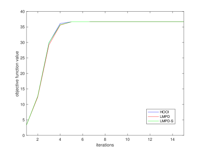
(a) ($r_{1},r_{2},r_{3}$) = (1,1,2)

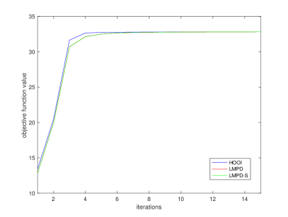
(b) $(r_{1},r_{2},r_{3}$) = (3,3,3)

​​​

Figure 1. Results for the tensor randomly generated in Example 7.17.

Example 7.18.

We randomly generate two tensors in $\mathbb{C}^{10\times 10\times 10}$, and run HOOI, LMPD and LMPD-S ($\gamma=0.01$) with ($r_{1},r_{2},r_{3}$) = (1,1,2). The distances of successive iterates $\|\omega^{(k,i+1)}-\omega^{(k,i)}\|$ are shown in Figure 2. It can be seen that HOOI and LMPD fail to converge globally, while LMPD-S has a much better convergence performance.

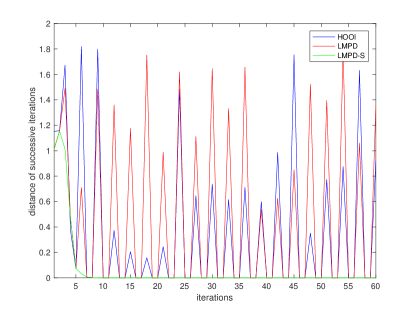
(a) first tensor

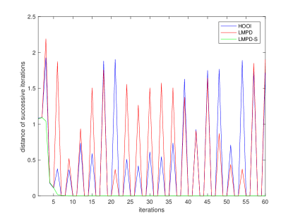
(b) second tensor

​​​

Figure 2. Results for the tensors randomly generated in Example 7.18.

8. Conclusions

Motivated by the objective functions (6) and (8), which are defined on the product of complex Stiefel manifolds and have wide applications in tensor approximation, in the general setting, we propose Algorithm APDOI and its shifted version APDOI-S to solve optimization over the product of complex Stiefel manifolds based on the matrix polar decomposition. When the general objective function (1) is multiconvex, we establish their weak convergence and global convergence based on the Łojasiewicz gradient inequality. Then, based on the Morse-Bott property, we prove the linear convergence rate, when the limit is a scale (or unitarily) semi-nondegenerate point. In particular, we show that the objective functions (6) and (8) are both multiconvex.

As the symmetric variant, for objective function (7), which has wide applications in symmetric tensor approximation, in the general setting, we propose Algorithm PDOI and its shifted version PDOI-S to solve optimization over a single complex Stiefel manifold based on the matrix polar decomposition. When the general objective function (5) is convex, we similarly establish their weak convergence, global convergence and linear convergence rate. We present examples in Example 6.9 to illustrate why the objective function (7) may be convex in many cases. It is a topic for further study to investigate if we can remove this assumption, while still guaranteeing convergence.

References

- [1] T. E. Abrudan, J. Eriksson, and V. Koivunen, Steepest descent algorithms for optimization under unitary matrix constraint, IEEE Trans. on Signal Process., 56 (2008), pp. 1134–1147.
- [2] P.-A. Absil, C. G. Baker, and K. A. Gallivan, Trust-region methods on Riemannian manifolds, Foundations of Computational Mathematics, 7 (2007), pp. 303–330.
- [3] P.-A. Absil, R. Mahony, and B. Andrews, Convergence of the iterates of descent methods for analytic cost functions, SIAM Journal on Optimization, 16 (2005), pp. 531–547.
- [4] P.-A. Absil, R. Mahony, and R. Sepulchre, Optimization algorithms on matrix manifolds, Princeton University Press, 2009.
- [5] P.-A. Absil, R. Mahony, and J. Trumpf, An extrinsic look at the Riemannian Hessian, in International Conference on Geometric Science of Information, Springer, 2013, pp. 361–368.
- [6] R. L. Adler, J.-P. Dedieu, J. Y. Margulies, M. Martens, and M. Shub, Newton’s method on Riemannian manifolds and a geometric model for the human spine, IMA Journal of Numerical Analysis, 22 (2002), pp. 359–390.
- [7] A. Anandkumar, R. Ge, D. Hsu, S. M. Kakade, and M. Telgarsky, Tensor decompositions for learning latent variable models, Journal of Machine Learning Research, 15 (2014), pp. 2773–2832.
- [8] D. P. Bertsekas, Nonlinear programming, Athena Scientific, second ed., 1999.
- [9] R. Bott, Nondegenerate critical manifolds, Annals of Mathematics, 60 (1954), pp. 248–261.
- [10] N. Boumal, B. Mishra, P.-A. Absil, and R. Sepulchre, Manopt, a Matlab toolbox for optimization on manifolds, Journal of Machine Learning Research, 15 (2014), pp. 1455–1459.
- [11] S. Boyd and L. Vandenberghe, Convex Optimization, Cambridge University Press, 2004.
- [12] D. Brandwood, A complex gradient operator and its application in adaptive array theory, IEE Proceedings H-Microwaves, Optics and Antennas, 130 (1983), pp. 11–16.
- [13] B. Chen, S. He, Z. Li, and S. Zhang, Maximum block improvement and polynomial optimization, SIAM Journal on Optimization, 22 (2012), pp. 87–107.
- [14] J. Chen and Y. Saad, On the tensor SVD and the optimal low rank orthogonal approximation of tensors, SIAM Journal on Matrix Analysis and Applications, 30 (2009), pp. 1709–1734.
- [15] A. Cichocki, D. Mandic, L. D. Lathauwer, G. Zhou, Q. Zhao, C. Caiafa, and H. A. PHAN, Tensor decompositions for signal processing applications: From two-way to multiway component analysis, IEEE Signal Processing Magazine, 32 (2015), pp. 145–163.
- [16] P. Comon, Independent Component Analysis, in Higher Order Statistics, J.-L. Lacoume, ed., Elsevier, Amsterdam, London, 1992, pp. 29–38.
- [17] P. Comon, Independent component analysis, a new concept?, Signal Processing, 36 (1994), pp. 287–314.
- [18] P. Comon, Tensor diagonalization, a useful tool in signal processing, IFAC Proceedings Volumes, 27 (1994), pp. 77–82.
- [19] P. Comon, Tensors: a brief introduction, IEEE Signal Processing Magazine, 31 (2014), pp. 44–53.
- [20] P. Comon, G. Golub, L.-H. Lim, and B. Mourrain, Symmetric tensors and symmetric tensor rank, SIAM Journal on Matrix Analysis and Applications, 30 (2008), pp. 1254–1279.
- [21] P. Comon and C. Jutten, eds., Handbook of Blind Source Separation, Academic Press, Oxford, 2010.
- [22] L. De Lathauwer, Signal processing based on multilinear algebra, Katholieke Universiteit Leuven, 1997.
- [23] L. De Lathauwer, P. Comon, B. De Moor, and J. Vandewalle, Higher-order power method - application in independent component analysis, in Proc. of the International Symposium on Nonlinear Theory and its Applications (NOLTA’95), 1995, pp. 91–96.
- [24] L. De Lathauwer, B. De Moor, and J. Vandewalle, On the best rank-1 and rank-(r1 ,r2 ,. . .,rn) approximation of higher-order tensors, SIAM Journal on Matrix Analysis and Applications, 21 (2000), pp. 1324–1342.
- [25] A. Edelman, T. A. Arias, and S. T. Smith, The geometry of algorithms with orthogonality constraints, SIAM Journal on Matrix Analysis and Applications, 20 (1998), pp. 303–353.
- [26] P. Feehan, Optimal Łojasiewicz-Simon inequalities and Morse-Bott Yang-Mills energy functions, arXiv:1706.09349, (2018).
- [27] G. H. Golub and C. F. Van Loan, Matrix Computations, Johns Hopkins University Press, 2012.
- [28] N. J. Higham, Functions of matrices: theory and computation, vol. 104, SIAM, 2008.
- [29] R. A. Horn and C. R. Johnson, Matrix Analysis, Cambridge University Press, 2012.
- [30] G. Hu, Y. Hua, Y. Yuan, Z. Zhang, Z. Lu, S. S. Mukherjee, T. M. Hospedales, N. M. Robertson, and Y. Yang, Attribute-enhanced face recognition with neural tensor fusion networks, in Proceedings of the IEEE International Conference on Computer Vision, 2017, pp. 3744–3753.
- [31] J. Hu, X. Liu, Z. Wen, and Y. Yuan, A brief introduction to manifold optimization, Journal of the Operations Research Society of China, (2020).
- [32] S. Hu and G. Li, Convergence rate analysis for the higher order power method in best rank one approximations of tensors, Numerische Mathematik, 140 (2018), pp. 993–1031.
- [33] S. Hu and K. Ye, Linear convergence of an alternating polar decomposition method for low rank orthogonal tensor approximations, arXiv:1912.04085, (2019).
- [34] M. Ishteva, Numerical methods for the best low multilinear rank approximation of higher-order tensors, PhD thesis, Department of Electrical Engineering, Katholieke Universiteit Leuven, (2009).
- [35] M. Ishteva, P.-A. Absil, and P. Van Dooren, Jacobi algorithm for the best low multilinear rank approximation of symmetric tensors, SIAM Journal on Matrix Analysis and Applications, 2 (2013), pp. 651–672.
- [36] M. Ishteva, P.-A. Absil, S. Van Huffel, and L. De Lathauwer, Best low multilinear rank approximation of higher-order tensors, based on the Riemannian trust-region scheme, SIAM Journal on Matrix Analysis and Applications, 32 (2011), pp. 115–135.
- [37] B. Jiang, Z. Li, and S. Zhang, Characterizing real-valued multivariate complex polynomials and their symmetric tensor representations, SIAM Journal on Matrix Analysis and Applications, 37 (2016), pp. 381–408.
- [38] M. Journée, Y. Nesterov, P. Richtárik, and R. Sepulchre, Generalized power method for sparse principal component analysis, Journal of Machine Learning Research, 11 (2010).
- [39] A. Karami, M. Yazdi, and G. Mercier, Compression of hyperspectral images using discerete wavelet transform and tucker decomposition, IEEE Journal of Selected Topics in Applied Earth Observations and Remote Sensing, 5 (2012), pp. 444–450.
- [40] E. Kofidis and P. A. Regalia, On the best rank-1 approximation of higher-order supersymmetric tensors, SIAM Journal on Matrix Analysis and Applications, 23 (2002), pp. 863–884.
- [41] T. G. Kolda, Orthogonal tensor decompositions, SIAM Journal on Matrix Analysis and Applications, 23 (2001), pp. 243–255.
- [42] T. G. Kolda and B. W. Bader, Tensor decompositions and applications, SIAM Review, 51 (2009), pp. 455–500.
- [43] T. G. Kolda and J. R. Mayo, Shifted power method for computing tensor eigenpairs, SIAM Journal on Matrix Analysis and Applications, 32 (2011), pp. 1095–1124.
- [44] A. Kovnatsky, K. Glashoff, and M. M. Bronstein, Madmm: a generic algorithm for non-smooth optimization on manifolds, in European Conference on Computer Vision, Springer, 2016, pp. 680–696.
- [45] S. Krantz and H. Parks, A Primer of Real Analytic Functions, Birkhäuser Boston, 2002.
- [46] S. G. Krantz, Function theory of several complex variables, vol. 340, American Mathematical Soc., 2001.
- [47] J. B. Kruskal, Rank, decomposition, and uniqueness for 3-way and n-way arrays, Multiway Data Analysis, (1989), pp. 7–18.
- [48] S. law Lojasiewicz, Ensembles semi-analytiques, IHES notes, (1965).
- [49] J. Li, K. Usevich, and P. Comon, Globally convergent Jacobi-type algorithms for simultaneous orthogonal symmetric tensor diagonalization, SIAM Journal on Matrix Analysis and Applications, 39 (2018), pp. 1–22.
- [50] J. Li, K. Usevich, and P. Comon, Jacobi-type algorithm for low rank orthogonal approximation of symmetric tensors and its convergence analysis, arXiv:1911.00659, (2019).
- [51] J. Li, K. Usevich, and P. Comon, On approximate diagonalization of third order symmetric tensors by orthogonal transformations, Linear Algebra and its Applications, 576 (2019), pp. 324–351.
- [52] J. Li, K. Usevich, and P. Comon, On the convergence of Jacobi-type algorithms for independent component analysis, in 11th IEEE Sensor Array and Multichannel Signal Processing Workshop, IEEE, 2020.
- [53] J. Li, X.-P. Zhang, and T. Tran, Point cloud denoising based on tensor tucker decomposition, in 2019 26th IEEE International Conference on Image Processing (ICIP), IEEE, 2019.
- [54] Z. Li, A. Uschmajew, and S. Zhang, On convergence of the maximum block improvement method, SIAM Journal on Optimization, 25 (2015), pp. 210–233.
- [55] S. Łojasiewicz, Sur la géométrie semi- et sous-analytique, Annales de l’institut Fourier, 43 (1993), pp. 1575–1595.
- [56] J. H. Manton, Modified steepest descent and Newton algorithms for orthogonally constrained optimisation. part i. the complex Stiefel manifold, in Proceedings of the Sixth International Symposium on Signal Processing and its Applications, vol. 1, IEEE, 2001, pp. 80–83.
- [57] J. Nie and Z. Yang, Hermitian tensor decompositions, arXiv:1912.07175, (2019).
- [58] J. Pan and M. K. Ng, Symmetric orthogonal approximation to symmetric tensors with applications to image reconstruction, Numerical Linear Algebra with Applications, 25 (2018), p. e2180.
- [59] B. T. Polyak, Gradient methods for minimizing functionals, Zh. Vychisl. Mat. Mat. Fiz., 3 (1963), pp. 643–653.
- [60] L. Qi and Z. Luo, Tensor analysis: Spectral theory and special tensors, SIAM, 2017.
- [61] L. Qi, F. Wang, and Y. Wang, Z-eigenvalue methods for a global polynomial optimization problem, Mathematical Programming, 118 (2009), pp. 301–316.
- [62] H. Sato and T. Iwai, A Riemannian optimization approach to the matrix singular value decomposition, SIAM Journal on Optimization, 23 (2013), pp. 188–212.
- [63] R. Schneider and A. Uschmajew, Convergence results for projected line-search methods on varieties of low-rank matrices via łojasiewicz inequality, SIAM Journal on Optimization, 25 (2015), pp. 622–646.
- [64] X. Shen, S. Diamond, M. Udell, Y. Gu, and S. Boyd, Disciplined multi-convex programming, in 2017 29th Chinese Control And Decision Conference (CCDC), IEEE, 2017, pp. 895–900.
- [65] N. D. Sidiropoulos, L. De Lathauwer, X. Fu, K. Huang, E. E. Papalexakis, and C. Faloutsos, Tensor decomposition for signal processing and machine learning, IEEE Transactions on Signal Processing, 65 (2017), pp. 3551–3582.
- [66] S. T. Smith, Optimization techniques on Riemannian manifolds, Fields Institute Communications, 3 (1994).
- [67] P. Tseng, Convergence of a block coordinate descent method for nondifferentiable minimization, Journal of Optimization Theory and Applications, 109 (2001), pp. 475–494.
- [68] L. R. Tucker, Some mathematical notes on three-mode factor analysis, Psychometrika, 31 (1966), pp. 279–311.
- [69] A. Uschmajew, A new convergence proof for the higher-order power method and generalizations, Pac. J. Optim., 11 (2015), pp. 309–321.
- [70] K. Usevich, J. Li, and P. Comon, Approximate matrix and tensor diagonalization by unitary transformations: convergence of Jacobi-type algorithms, arXiv:1905.12295v2, (2020).
- [71] A. Van Den Bos, Complex gradient and Hessian, IEE Proceedings-Vision, Image and Signal Processing, 141 (1994), pp. 380–382.
- [72] Z. Wen and W. Yin, A feasible method for optimization with orthogonality constraints, Mathematical Programming, 142 (2013), pp. 397–434.
- [73] S. J. Wright, Accelerated block-coordinate relaxation for regularized optimization, SIAM Journal on Optimization, 22 (2012), pp. 159–186.
- [74] Y. Xu, On the convergence of higher-order orthogonal iteration, Linear and Multilinear Algebra, 66 (2018), pp. 2247–2265.
- [75] Y. Xu and W. Yin, A block coordinate descent method for regularized multiconvex optimization with applications to nonnegative tensor factorization and completion, SIAM Journal on Imaging Sciences, 6 (2013), pp. 1758–1789.
- [76] Y. Yang, The epsilon-alternating least squares for orthogonal low-rank tensor approximation and its global convergence, arXiv:1911.10921, (2019).
- [77] T. Zhang and G. H. Golub, Rank-one approximation to high order tensors, SIAM Journal on Matrix Analysis and Applications, 23 (2001), pp. 534–550.
- [78] X. Zhang, C. Ling, and L. Qi, The best rank-1 approximation of a symmetric tensor and related spherical optimization problems, SIAM Journal on Matrix Analysis and Applications, 33 (2012), pp. 806–821.