Extensionless Adaptive Transmitter and Receiver Windowing of Beyond 5G Frames

Abstract

Newer cellular communication generations are planned to allow asynchronous transmission of multiple numerologies (waveforms with different parameters) in adjacent bands, creating unavoidable adjacent channel interference. Most prior work on windowing assume additional extensions reserved for windowing, which does not comply with standards. Whether windowing should be applied at the transmitter or the receiver was not questioned. In this work, we propose two independent algorithms that are implemented at the transmitter and receiver, respectively. These algorithms estimate the transmitter and receiver windowing duration of each resource element (RE) with an aim to improve fair proportional network throughput. While doing so, we solely utilize the available extension that was defined in the standard and present standard-compliant algorithms that also do not require any modifications on the counterparts or control signaling. Furthermore, computationally efficient techniques to apply per-RE transmitter and receiver windowing to signals synthesized and analyzed using conventional cyclic prefix-orthogonal frequency division multiplexing are derived and their computational complexities are analyzed. The spectrotemporal relations between optimum window durations at either side, as well as functions of the excess signal-to-noise ratios, the subcarrier spacings and the throughput gains provided over previous similar techniques are numerically verified.

I Introduction

Third Generation Partnership Project (3GPP) designed 4G- Long Term Evolution (LTE) to deliver broadband services to masses[1]. The design was successful in doing what it promised, but the one-size-fits-all approach resulted in certain engineering trade-offs. This broadband experience was possible at a certain reliability not allowing ultra reliable and low latency communications (uRLLC) operations, is not the most power-efficient design and is only possible below $120\text{\,}\mathrm{km}\text{/}\mathrm{h}$ mobility[2]. 5G new radio (NR) physical layer was designed to utilize the orthogonal frequency division multiplexing (OFDM) waveform[3] with different parameters, called numerologies, allowing prioritization of certain aspects in different applications and made the enhanced-mobile broadband (eMBB) experience possible in a wider range of scenarios[4]. For example, while low power Internet of Things (IoT) devices are assigned smaller subcarrier spacings to conserve battery, vehicular communications are operating with higher subcarrier spacings and shorter symbol durations to keep the communication reliable in high Doppler spreads caused by higher speeds.

This shift in paradigm brought with it a problem deliberately avoided by the uniform design. Regardless of the domain multiple accessing (MA) was performed, the use of a unified orthogonal waveform in the point-to-multipoint downlink (DL) avoided the inter- user equipment (UE) interference problem experienced in the multipoint-to-point uplink (UL) in all preceding generations of cellular communications. However, by allowing coexistence of different OFDM numerologies in adjacent bands, adjacent channel interference (ACI) between UEs sharing these bands arises in the DL[5]. In the UL, although orthogonal waveforms were used in principle, power differences and timing and frequency offsets across UEs caused interference. Although they came at certain costs, strict timing and frequency synchronization across UEs[6] and power control[7] have been historically used to mitigate the interference in the UL. Unfortunately, with the use of different numerologies, these remedies are not a solution to the problem and inter-numerology interference (INI) is inevitable[8] even in the DL. 3GPP acknowledges this problem and gives manufacturers the freedom to implement any solution they choose as long as they respect the standard frame structure[9] seen in Fig. 1a.

Windowing of OFDM signals is a well-studied interference management technique that has garnered attention due to its low computational complexity. Windowing can be performed independently at the transmitter to reduce out-of-band (OOB) emission[10], or at the receiver to reduce interference caused by communication taking place in adjacent channels, commonly referred to as ACI [11]. Most recently in [12], utilizing different window functions for each subcarrier at the transmitter and receiver is proposed and the window functions for each subcarrier that maximizes the spectral localization within the UE’s resources and interference rejection are derived.

In [12] and most of the preceding literature focusing on windowing, windowing was performed by extending the symbols by an amount which was arbitrarily chosen without explanation, in addition to standard cyclic prefix (CP) duration seen in Fig. 1b, and the focus was on deriving window functions optimized according to maximize standard performance metrics. These extensions reduce the symbol rate and change the frame structure defined in the standard, thus creating nonstandard signals that are not orthogonal to the symbols that aims to share the same numerology[5]. As mentioned above, this is not acceptable in the current cellular communication standards[9]. Furthermore, extending the symbol duration relentlessly causes the symbol duration to exceed the coherence time of the channel, which is a critical problem for high-speed vehicular communications[5]. In [13], the authors attempted to improve spectral efficiency of windowed OFDM systems by not applying windowing to the REs of inner subcarriers assigned to UEs experiencing long delay spreads and applying windowing on the edge subcarriers using the excess CP assigned to UEs experiencing short delay spreads. While effective, this scheme is only applicable if all UEs utilize the same numerology. The first standard compliant windowing scheme was proposed in [14], in which the authors derived the receiver windowing durations that optimize reception of each subcarrier in the case which intersymbol interference (ISI) and ACI occur simultaneously and pulse shapes of transmitters operating in adjacent bands cannot be controlled, in the absence of any extension designated for windowing. Whether it is more beneficial to window a duration at the transmitter or receiver was not discussed in the literature.

This work aims to extend [14] by evaluating how network capacity can be further improved if the pulse shapes of the transmitted waveforms can also be designed while conserving the standard frame structure, that is, not adding any additional extensions other than CP and using only the present CP for windowing. In this work, we propose two independent algorithms that aim to determine the amount of windowing that should be applied at either side to maximize fair proportional network capacity. Unlike [14] in which receiver windowing duration calculations required channel impulse responses knowledge, the proposed receiver windowing duration calculation algorithm in this work is solely uses statistics derived from the received signals. This significantly reduces the complexity and eases implementation, and makes the algorithm completely practical as no information is needed. The proposed transmitter windowing duration calculation algorithm aims to maximize the network spectral efficiency by assigning high transmit window durations only to REs with excess signal to interference plus noise ratio (SINR) that can withstand the ISI caused by windowing. This reduces the ACI in the system with minimum impact to the REs applying windowing. Neither algorithm requires any control data transfer to other parties of the communication or changes to the other nodes at any point. The proposed utilization of the standard symbol structure as a function of excess signal-to-noise ratio (SNR) is shown in Fig. 1c. Numerical results confirm that fair proportional network spectral efficiency can be increased greatly without disrupting the standard frame structure by utilizing CP adaptively, and determining transmitter windowing durations using excess SINR of REs and data-aided receiver windowing duration determination are an effective metrics.

(a)

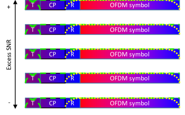
(b)

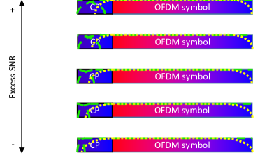
(c)

Figure 1: Visual demonstrations of temporal (a) standard symbol structure, (b) structure used in previous windowing literature and (c) the adaptive CP concept presented in this work. The rectangles are alotted times for the actual OFDM symbol, CP, and further cyclic extensions for “T”ransmitter and “R”eceiver windowing, while the green dash and yellow round dot overlays demonstrate transmitter and receiver windowing of the underlying area, respectively.

Our contributions in this work are as follows:

• Computationally efficient per-RE transmitter and receiver windowing of signals synthesized and analyzed using conventional CP-OFDM are derived.

• A computationally efficient per-RE transmitter window duration estimation algorithm for next generation NodeBs that maximizes the fair proportional network throughput based on UEs channel conditions and does not require any information transfer to or modification at UEs is presented.

• A computationally efficient per-RE receiver window duration estimation algorithm for gNBs and UEs that maximizes the capacity of each RE and does not require any information transfer from or modification at the transmitter is presented.

• The computational complexities of the aforementioned algorithms are derived.

• The algorithms are numerically analyzed in terms of OOB-emission reduction, throughput improvements, relation of window duration estimates with excess SNR, spectrotemporal correlation and accuracy of window duration estimates.

Notation: ${\left(\cdot\right)}^{\mkern-1.5mu\mathsf{T}}$, ${\left(\cdot\right)}^{\mkern-1.5mu\ast}$ and ${\left(\cdot\right)}^{\mkern-1.5mu\mathsf{H}}$ denote the transpose, conjugate and Hermitian operations, $\mathbf{\bm{A}}\left[a,b\right]$ is the element in the $a$th row and $b$th column of matrix $\mathbf{\bm{A}}$, $\mathbf{\bm{A}}\left[a,:\right]$ and $\mathbf{\bm{A}}\left[:,b\right]$ are each row and column vectors containing the $a$th row and $b$th column of matrix $\mathbf{\bm{A}}$, respectively, $\operatorname{vec}{\left(\mathbf{\bm{A}}\right)}={\begin{bmatrix}{\mathbf{\bm{A}}\left[:,1\right]}^{\mkern-1.5mu\mathsf{T}}&{\mathbf{\bm{A}}\left[:,2\right]}^{\mkern-1.5mu\mathsf{T}}&\dots\end{bmatrix}}^{\mkern-1.5mu\mathsf{T}}$ is the vectorization operator, $\mathbf{\bm{A}}\odot\mathbf{\bm{B}}$ and $\mathbf{\bm{A}}\oslash\mathbf{\bm{B}}$ correspond to Hadamard multiplication and division of matrices $\mathbf{\bm{A}}$ and $\mathbf{\bm{B}}$ and $\mathbf{\bm{A}}$ by $\mathbf{\bm{B}}$, $\mathbf{\bm{0}}_{A\times B}$ denotes matrices of zeros with $A$ rows and $B$ columns, $\mathcal{CN}\left(\mu,\sigma^{2}\right)$ represents complex Gaussian random processes with mean $\mu$ and variance $\sigma^{2}$, $\lfloor\mathbf{\bm{X}}\rceil$ correspond to rounding all elements of $\mathbf{\bm{X}}$ to the nearest integer, $\#\mathbb{S}$ denotes the cardinality of set $\mathbb{S}$, $\operatorname{E}_{x}\left[\mathbf{\bm{y}}\right]$ is the expected value of random vector $\mathbf{\bm{y}}$ with respect to variable $x$, and $\jmath=\sqrt{-1}$.

II System Model

In this work, we assume that there is a node, referred to as the gNB, that conveys information to all other nodes in the system and all other nodes aim to convey information solely to the gNB during processes referred to as DL and UL, respectively. There are $U$ nodes other than the gNB, hereinafter referred to as UEs, sharing a total bandwidth $B$ to communicate with the gNB using OFDM. Each UE $u$ samples this whole band band using an $N_{u}$-point fast Fourier transformation (FFT), such that the frequency spacing between the points at the FFT output becomes $\Delta f_{u}=B/N_{u}$. The quantity $\Delta f_{u}$ is referred to as the subcarrier spacing of UE $u$. Bi-directional communication takes place in a time domain duplexing (TDD) fashion and frequency division multiple accessing (FDMA) is used for multiple accessing; UEs solely receive and do not transmit during gNB’s transmission, i.e. DL, whereas all UEs transmit simultaneously in adjacent but non-overlapping frequency bands in the UL. UL is assumed to take place before DL and is crucial to the work, but we focus on modeling the details of the DL necessary for the proposed methods for sake of brevity, while necessary details regarding UL are provided in numerical verification. The data of each UE $u$ is conveyed in $M_{u}$ consecutive subcarriers of $L_{u}$ consecutive OFDM symbols, with contiguous indices $\left\{M_{u,1},\dots,M_{u,M_{u}}\right\}$ out of the possible $N_{u}$, while the remaining subcarriers are left empty for use by other UEs. Although the algorithms presented and performed analysis are directly compatible with orthogonal frequency division multiple accessing (OFDMA), for the sake of simplifying the notation throughout this work, we assume pure FDMA, that is, $L_{u_{1}}N_{u_{1}}=L_{u_{2}}N_{u_{2}}\,,\forall u_{1},u_{2}\in\mathbb{N}_{\leq U}^{*}$.

Symbols known by receiving nodes, commonly referred to as pilot or demodulation reference signal (DMRS), are transmitted in some REs for time synchronization and channel estimation purposes in both UL and DL. The DMRS transmitted to UE $u$ are contained in the sparse matrix $\mathbf{\bm{P}}_{u}\in\mathbb{C}^{M_{u}\times L_{u}}$. The single carrier (SC) data symbols transmitted to UE $u$ are contained in $\mathbf{\bm{D}}_{u}\in\mathbb{C}^{M_{u}\times L_{u}}$, of which nonzero elements do not overlap with that of $\mathbf{\bm{P}}_{u}$.

A CP of length $K_{u}$ samples is appended to the each time domain OFDM symbol to mitigate multipath propagation and prevent ISI, where $K_{u}/L_{u}$ equals to the same constant for all UEs of the network and is referred to as the CP rate. The OFDM symbol samples, preceded their respective CP samples to be broadcasted to all users can be obtained as

$$\breve{\mathbf{\bm{x}}}=\sum_{u=1}^{U}\operatorname{vec}{\left(\begin{bmatrix}\begin{array}[]{cc}\mathbf{\bm{0}}_{K_{u}\times\left(N_{u}-K_{u}\right)}&\mathbf{\bm{I}}_{K_{u}}\end{array}\\ \mathbf{\bm{I}}_{N_{u}}\end{bmatrix}\mathbf{\bm{F}}_{N_{u}}\mathbf{\bm{Q}}_{u}\left(\mathbf{\bm{P}}_{u}+\mathbf{\bm{D}}_{u}\right)\right)},$$ (1)

where $\breve{\mathbf{\bm{x}}}\in\mathbb{C}^{\left(N_{u}+K_{u}\right)L_{u}\times 1,\,\forall u}$ is the basic baseband sample sequence, $\mathbf{\bm{Q}}_{u}\in\mathbb{R}^{N_{u}\times M_{u}}$ is the resource mapping matrix of $u$th UE that maps the data elements to the scheduled resources, and $\mathbf{\bm{F}}_{N_{u}}\in\mathbb{C}^{N_{u}\times N_{u}}$ is the normalized $N_{u}$-point FFT matrix. Some CP samples may also be used for transmitter windowing to limit the OOB emission as described in [12, 15]. Different transmitter window durations may be utilized for each RE to be transmitted to each UE. The transmitter window durations associated with $u$th UE’s REs are given in $\mathbf{\bm{T}}_{u}\in\mathbb{N}_{\leq K_{u}}^{M_{u}\times L_{u}}$ and calculated according to Section III-A. Let $\mathbf{\bm{x}}\in\mathbb{C}^{\left(\left(K_{u}+N_{u}\right)L_{u}\right)\times 1}$ denote the per-RE transmitter windowed baseband sample sequence, calculated computationally efficiently as described in Section III-A.

The waveform is then transmitted over the multiple access multipath channel. The complex channel gain of the cluster that arrives at the $u$th UE at the $t$th sample after a delay of $\tau$ samples is denoted by the complex coefficient $h_{u,\tau,t}$. We assume that these channel gains are normalized such that $\mathbb{E}_{t}\left[\sum_{\tau=0}^{t-\Delta_{t,u}-1}\left|h_{u,\tau,t}\right|^{2}\right]=1$ and that they vary at each sample instant where the mobility of each UE is independent of all others. Then, the $t$th sample received at $u$th UE is written as

$$\mathbf{\bm{y}}_{u}\left[t\right]=\tilde{n}+\sqrt{\gamma_{u}}\sum_{\tau=0}^{t-\Delta_{t,u}-1}h_{u,\tau,t}\mathbf{\bm{x}}\left[t-\Delta_{t,u}-\tau\right],\,t\in\mathbb{N}^{*},$$ (2)

where $\mathbf{\bm{x}}\left[t\right]\coloneqq 0,\,\forall t\in\mathbb{N}_{>\left(K_{u}+N_{u}\right)L_{u}}\cup\mathbb{Z}^{-}$, $\tilde{n}\sim\mathcal{CN}\left(0,1\right)$ is the background additive white Gaussian noise (AWGN), $\gamma_{u}$ is the overall SNR of $u$th UE and $\Delta_{t,u}$ is the propagation delay for $u$th UE in number of samples. Each UE then synchronizes to their signal by correlating the received samples with samples generated only using their $\mathbf{\bm{P}}_{u}$ and estimates $\hat{\Delta_{t,u}}$[16]. The samples estimated to contain $u$th UE’s $l$th OFDM symbol and its corresponding CP is denoted by vector $\mathbf{\bm{y}}_{l,u}\in\mathbb{C}^{\left(K_{u}+N_{u}\right)\times 1}$, where $\mathbf{\bm{y}}_{l,u}\left[s\right]=\mathbf{\bm{y}}_{u}\left[\left(l-1\right)\left(N_{u}+K_{u}\right)+\hat{\Delta_{t,u}}+s\right],\,s\in\mathbb{N}_{\leq\left(K_{u}+N_{u}\right)}^{*}$. Before the receiver windowing operations are performed, $u$th UE first performs regular OFDM reception and calculates the received SC symbols from the OFDM symbol samples as

$$\mathbf{\bm{Y}}_{u}\left[:,l,0\right]={\mathbf{\bm{Q}}_{u}}^{\mkern-1.5mu\mathsf{T}}\mathbf{\bm{F}}_{N_{u}}\begin{bmatrix}\mathbf{\bm{0}}_{N_{u}\times K_{u}}&\mathbf{\bm{I}}_{N_{u}}\end{bmatrix}\mathbf{\bm{y}}_{l,u}^{\text{}},$$ (3)

where the first plane of $\mathbf{\bm{Y}}_{u}\in\mathbb{C}^{M_{u}\times L_{u}\times\left(K_{u}+1\right)}$ are the received base SC symbols. Each UE uses a different receiver window duration to receive each RE. The receiver window durations associated with $u$th UE’s REs are given in $\mathbf{\bm{R}}_{u}\in\mathbb{N}_{\leq K_{u}}^{M_{u}\times L_{u}}$ and are calculated according to Section III-B, wherein also the calculation of the receiver windowed SC symbols $\hat{\mathbf{\bm{Y}}}_{u}\in\mathbb{C}^{M_{u}\times L_{u}}$ are demonstrated. channel frequency response (CFR) coefficients at DMRS locations are first estimated as

$$\breve{\mathbf{\bm{H}}}_{u}\left[m,l\right]=\hat{\mathbf{\bm{Y}}}_{u}\left[m,l\right]\oslash\mathbf{\bm{P}}_{u}\left[m,l\right]$$ (4)

using nonzero elements of $\mathbf{P}_{u}$. Then, a transform domain channel estimator [17, (33)] is applied and estimated CIRs are reduced to their first $K_{u}$ coefficients. The CIR coefficients of non-pilot carrying symbols are interpolated and extrapolated[18], and all CFR coefficient estimates $\hat{\mathbf{\bm{H}}}_{u}$ are obtained[17, (33)]. Finally, data symbols are equalized as described in [19] for nonzero elements of $\mathbf{D}_{u}$ and the received symbols are estimated as

$$\hat{\mathbf{D}}_{u}=\frac{\hat{\mathbf{\bm{Y}}}_{u}\odot{\text{$\hat{\mathbf{\bm{H}}}$}}^{\mkern-1.5mu\ast}_{u}}{\hat{\bm{\sigma}}_{\text{n},u}^{2}+\text{$\hat{\mathbf{\bm{H}}}_{u}$}\odot{\text{$\hat{\mathbf{\bm{H}}}$}}^{\mkern-1.5mu\ast}_{u}},$$ (5)

where $\hat{\bm{\sigma}}_{\text{n},u}^{2}\in\mathbb{R}^{M_{u}\times L_{u}}$ is the variance estimated by $u$th UE for noise, various interference sources and other disruptions.

III Proposed Method

The idea proposed in this work involves determination of $\mathbf{\bm{T}}_{u}$ and $\mathbf{\bm{R}}_{u}$ for all UEs that maximizes the fair-proportional network capacity. Because these concepts are implemented independently, they are discussed separately.

III-A Estimation of Optimum Transmitter Window Durations

This subsection first discusses efficient differential calculation of per-RE transmitter windowed samples to prove the optimum transmitter window durations calculations feasible. The optimization metric, fair proportional network capacity, is then defined. An algorithm to effectively maximize the fair proportional network capacity is provided. Finally, the computational complexity of the provided algorithm is calculated and discussed.

III-A1 Computationally Efficient Conversion of Conventional CP-OFDM Samples to Per-RE Transmitter Windowed OFDM Samples

The transmit pulse shape of the $m$th subcarrier of $l$th OFDM symbol to be transmitted to UE $u$ in accordance with $\mathbf{\bm{T}}_{u}\left[m,l\right]$ is contained in the vector $\mathbf{\bm{t}}_{m,l,u}\in\mathbb{R}^{\left(K_{u}+N_{u}+T_{u}\right)\times 1}$ of which indexing is demonstrated in Fig. 2 and is calculated per [12] to contain the energy of that subcarrier within the band assigned to the UE. Investigating (1), if no transmitter windowing is applied, i.e. the generation of a regular CP-OFDM sample sequence $\breve{\mathbf{\bm{x}}}$, the contribution from the symbol in the $m$th subcarrier of the $l$th OFDM symbol of $u$th user to the $k\leq K_{u}$th sample of that OFDM symbol is $\exp\left(-\jmath 2\pi M_{u,m}\left(k-K_{U}-1\right)/N_{u}\right)\left(\mathbf{\bm{D}}_{u}\left[m,l\right]+\mathbf{\bm{P}}_{u}\left[m,l\right]\right)/\sqrt{N_{u}}$. If transmitter windowing is applied to the RE in interest, the contribution at $k\leq\mathbf{\bm{T}}_{u}\left[m,l\right]$th sample would instead become

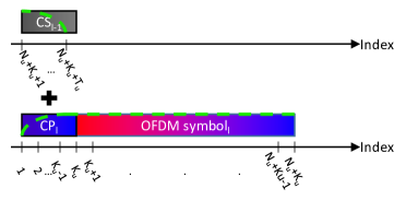
Figure 2: Indexing of $\mathbf{\bm{t}}$ within a demonstration of how transmitter windowed samples are generated by overlapping scaled CP of current and CS of preceding OFDM symbols of which indices are given in the subscripts.

$\left(\mathbf{\bm{t}}_{m,l,u}\left[k\right]\exp\left(-\jmath\tfrac{2\pi M_{u,m}\left(k-1-K_{U}\right)}{N_{u}}\right)\left(\mathbf{\bm{D}}_{u}\left[m,l\right]+\mathbf{\bm{P}}_{u}\left[m,l\right]\right)+\mathbf{\bm{t}}_{m,l,u}\left[k+N_{u}+K_{u}\right]\exp\left(-\jmath\tfrac{2\pi M_{u,m}\left(k-1\right)}{N_{u}}\right)\left(\mathbf{\bm{D}}_{u}\left[m,l-1\right]+\mathbf{\bm{P}}_{u}\left[m,l-1\right]\right)\right)/\sqrt{N_{u}}$$=\frac{\exp\left(-\jmath\tfrac{2\pi M_{u,m}\left(k-1\right)}{N_{u}}\right)}{\sqrt{N_{u}}}\left(\mathbf{\bm{t}}_{m,l,u}\left[k\right]\exp\left(\jmath\tfrac{2\pi M_{u,m}K_{U}}{N_{u}}\right)\left(\mathbf{\bm{D}}_{u}\left[m,l\right]+\mathbf{\bm{P}}_{u}\left[m,l\right]\right)+\mathbf{\bm{t}}_{m,l,u}\left[k+N_{u}+K_{u}\right]\left(\mathbf{\bm{D}}_{u}\left[m,l-1\right]+\mathbf{\bm{P}}_{u}\left[m,l-1\right]\right)\right).$ Noting that $\mathbf{\bm{t}}_{m,l,u}\left[k\right]\coloneqq 1-\mathbf{\bm{t}}_{m,l,u}\left[k+N_{u}+K_{u}\right],\,\forall k\in\mathbb{Z}_{\leq N_{u}+K_{u}}^{+}$[12, 15], the $k\leq T_{u}\left[m,l\right]$th sample of $u$th user’s $l$th OFDM symbol’s per-RE transmitter windowed $m$th subcarrier can be converted from that generated using a conventional CP-OFDM procedure as

$$\mathbf{\bm{x}}\left[\left(l-1\right)\left(N_{u}+K_{u}\right)+k\right]=\breve{\mathbf{\bm{x}}}\left[\left(l-1\right)\left(N_{u}+K_{u}\right)+k\right]+\tfrac{\mathbf{\bm{t}}_{m,l,u}\left[k+N_{u}+K_{u}\right]\exp\left(-\jmath\tfrac{2\pi M_{u,m}\left(k-1\right)}{N_{u}}\right)}{\sqrt{N_{u}}}\left(\left(\mathbf{\bm{D}}_{u}\left[m,l-1\right]+\mathbf{\bm{P}}_{u}\left[m,l-1\right]\right)-\exp\left(\jmath\tfrac{2\pi M_{u,m}K_{U}}{N_{u}}\right)\left(\mathbf{\bm{D}}_{u}\left[m,l\right]+\mathbf{\bm{P}}_{u}\left[m,l\right]\right)\right).$$ (6)

$\mathbf{\bm{x}}$ can be obtained by converting all $T_{u}\left[m,l\right]$ samples of $\breve{\mathbf{\bm{x}}}$ to per-RE transmitter windowed samples, and this is implied in all further references to (6).

III-A2 Estimation of Fair Proportional Network Capacity

In order to estimate the optimum transmitter window durations, the gNB first estimates the SINR and corresponding capacity for each RE of each user prior to transmission, calculates the fair proportional network capacity, and tries to increase it iteratively. The samples to be received at the $u$th UE are first estimated as

$$\hat{\mathbf{\bm{y}}}_{u}\left[t\right]=\sum_{\tau=0}^{t-1}\hat{h}_{u,\tau,t}\mathbf{\bm{x}}\left[t-\tau\right],\,t\in\mathbb{N}_{\leq\left(K_{u}+N_{u}\right)L_{u}}^{*},$$ (7)

where $\hat{h}_{u,\tau,t}$ are the CIR coefficient predictions[18] at the gNB prior to transmission. The samples are regrouped accordingly to $L_{u}$ groups of $K_{u}+N_{u}$ samples each and receiver processed as described in Section II, that is, CPs are removed from all symbols, FFTs are applied, and receiver windowing is performed if the gNB is aware that the receiver in current interest does so. Results for various cases of receiver windowing are provided in Section IV, but for the sake of brevity, we assume that the gNB assumes none of the UEs perform receiver windowing in the remainder of this subsection. The gNB estimate at the FFT output, $\tilde{\mathbf{\bm{Y}}}_{u}\in\mathbb{C}^{M_{u}\times L_{u}}$, is formulated as

$$\tilde{\mathbf{\bm{Y}}}_{u}\left[m,l\right]=\tilde{\mathbf{\bm{H}}}_{u}\left[m,l\right]\left(\mathbf{D}_{u}\left[m,l\right]+\tilde{\mathbf{D}}_{u}\left[m,l\right]\right),$$ (8)

where $\tilde{\mathbf{\bm{H}}}_{u}\left[m,l\right]$ is the CFR coefficient prediction of the $m$th subcarrier of the $l$th OFDM symbol of $u$th user, the first term inside parentheses is due to the data itself, and the second term inside parentheses shown as $\tilde{\mathbf{D}}_{u}$ is the cumulative ACI, inter-carrier interference (ICI) and ISI. Note that since the source samples for all these effects are summed with that of data at the gNB and are passed through the same channel, this cumulative disruption is also scaled with the same channel gain. Accordingly, the number of bits that can be conveyed in the actual noisy transmission channel using the data carrying $m$th subcarrier of the $l$th OFDM symbol of $u$th UE is [20]

$$\breve{\bm{\eta}}_{u}\left[m,l\right] =\log_{2}\left(1+\frac{\left|\tilde{\mathbf{\bm{H}}}_{u}\left[m,l\right]\right|^{2}}{1+\left|\tilde{\mathbf{\bm{H}}}_{u}\left[m,l\right]\right|^{2}\left|\tilde{\mathbf{D}}_{u}\left[m,l\right]\right|^{2}}\right)$$

$$=\log_{2}\left(1+\frac{\left|\tilde{\mathbf{\bm{H}}}_{u}\left[m,l\right]\right|^{2}}{1+\left|\tilde{\mathbf{\bm{Y}}}_{u}\left[m,l\right]-\tilde{\mathbf{\bm{H}}}_{u}\left[m,l\right]\mathbf{D}_{u}\left[m,l\right]\right|^{2}}\right).$$ (9)

If the RE under investigation is scheduled to use a certain modulation and coding scheme (MCS) to carry $\mathbf{\bm{b}}_{u}\left[m,l\right]$ bits, (9) is in fact capped as

$$\bm{\eta}_{u}\left[m,l\right]=\min\left(\mathbf{\bm{b}}_{u}\left[m,l\right],\breve{\bm{\eta}}_{u}\left[m,l\right]\right).$$ (10)

The mean number of bits conveyable to $u$th UE per RE is

$$\bar{\eta}_{u} =\operatorname{E}_{m}\left[\operatorname{E}_{l}\left[\bm{\eta}_{u}\left[m,l\right]\right]\right],$$ (11)

and we define the fair proportional network capacity as the geometric mean of the mean capacities of all UEs in the network

$$\eta=\sqrt[U]{\prod_{u=1}^{U}\bar{\eta}_{u}}.$$ (12)

III-A3 Optimum Transmitter Window Duration Estimation Algorithm

Given the discrete nature of possible window durations in digital pulse shaping and the lack of a relation between window duration and amount of interference incurred on a victim subcarrier for optimum window functions used in this work[12] for the time-varying multipath multiple access channel, an analytical solution to this multivariate integer optimization problem with such a nonlinear utility function is not obvious at the time of writing. The choice of transmitter window duration of any RE must balance the SINR degradation to the REs caused by induced ISI, and the SINR improvement to all other REs, particularly those of other UEs. The transmitter window duration affects the whole network, hence, must be calculated keeping the whole network in mind, meaning (12) must be calculated and optimized at the gNB prior to transmission. However, explicitly calculating eqs. 6, 7, 8, 9, 10, 11 and 12 every time for each RE is computationally exhaustive. The aforementioned equations are provided to provide the necessary understanding, but the following equations will be used in the computationally efficient estimation of optimum transmitter window durations. Consider that we wish to test whether setting the transmitter window duration of the RE in the $\dot{m}$th subcarrier of the $\dot{l}$th OFDM symbol of $\dot{u}$th user to $\mathbf{\bm{T}}_{\dot{u}}\left[\dot{m},\dot{l}\right]$ improves the fair proportional network capacity or not. Assume the transmitter windowed samples are calculated per (6). To keep expressions clear, let us refer to the difference in the $k$th CP sample in interest per (6) as

$$\dot{x}_{k}\coloneqq\mathbf{\bm{x}}\left[\left(\dot{l}-1\right)\left(N_{\dot{u}}+K_{\dot{u}}\right)+k\right]-\breve{\mathbf{\bm{x}}}\left[\left(\dot{l}-1\right)\left(N_{\dot{u}}+K_{\dot{u}}\right)+k\right]$$ (13)

$$=\tfrac{\mathbf{\bm{t}}_{\dot{m},\dot{l},\dot{u}}\left[k+N_{\dot{u}}+K_{\dot{u}}\right]\exp\left(-\jmath\tfrac{2\pi M_{\dot{u},\dot{m}}\left(k-1\right)}{N_{\dot{u}}}\right)}{\sqrt{N_{\dot{u}}}}\left(\left(\mathbf{\bm{D}}_{\dot{u}}\left[\dot{m},\dot{l}-1\right]+\mathbf{\bm{P}}_{\dot{u}}\left[\dot{m},\dot{l}-1\right]\right)-\exp\left(\jmath\tfrac{2\pi M_{\dot{u},\dot{m}}K_{\dot{U}}}{N_{\dot{u}}}\right)\left(\mathbf{\bm{D}}_{\dot{u}}\left[\dot{m},\dot{l}\right]+\mathbf{\bm{P}}_{\dot{u}}\left[\dot{m},\dot{l}\right]\right)\right).$$ (14)

The next step is to regenerate (8) for all UEs. However, as the number of changed symbols is limited, whole sample sequences do not need regeneration, but only the received samples that are affected by the changed samples, and fall into a valid receiver window must be recalculated. For example, assuming a conventional rectangular receiver window is utilized at the receivers, which will be assumed in the rest of this section, any changes to CP samples will be discarded as they fall outside the receiver window, hence need not be calculated. In this case, first $\mathbf{\bm{T}}_{\dot{u}}\left[\dot{m},\dot{l}\right]$ modified samples that the channel would leak into the symbol duration must be calculated for each UE, and the $k$th sample (per indexing of Fig. 2) of the transmitter windowed received sample sequence $\widehat{\mathbf{\bm{y}}_{u}}$ can be written as

$$\widehat{\mathbf{\bm{y}}_{u}}\left[\left(\dot{l}-1\right)\left(N_{\dot{u}}+K_{\dot{u}}\right)+k\right]=\sum_{\tau=0}^{K_{u}}\hat{h}_{u,\tau,\left(\dot{l}-1\right)\left(N_{\dot{u}}+K_{\dot{u}}\right)+k}\mathbf{\bm{x}}\left[\left(\dot{l}-1\right)\left(N_{\dot{u}}+K_{\dot{u}}\right)+k-\tau\right]$$ (15)

$$=\sum_{\tau=0}^{K_{u}}\hat{h}_{u,\tau,\left(\dot{l}-1\right)\left(N_{\dot{u}}+K_{\dot{u}}\right)+k}\left(\breve{\mathbf{\bm{x}}}\left[\left(\dot{l}-1\right)\left(N_{\dot{u}}+K_{\dot{u}}\right)+k-\tau\right]+\dot{x}_{k-\tau}\right)$$ (16)

$$=\hat{\mathbf{\bm{y}}}_{u}\left[\left(\dot{l}-1\right)\left(N_{\dot{u}}+K_{\dot{u}}\right)+k\right]+\sum_{\tau=k-\mathbf{\bm{T}}_{\dot{u}}\left[\dot{m},\dot{l}\right]}^{K_{u}}\hat{h}_{u,\tau,\left(\dot{l}-1\right)\left(N_{\dot{u}}+K_{\dot{u}}\right)+k}\dot{x}_{k-\tau}.$$ (17)

Let us similarly refer to the difference in the $k$th relevant (belonging to the OFDM symbol affected by the windowing operation) sample to be received by the $u$th UE as

$$\dot{y}_{u,k} =\widehat{\mathbf{\bm{y}}_{u}}\left[\left(\dot{l}-1\right)\left(N_{\dot{u}}+K_{\dot{u}}\right)+k\right]-\hat{\mathbf{\bm{y}}}_{u}\left[\left(\dot{l}-1\right)\left(N_{\dot{u}}+K_{\dot{u}}\right)+k\right]$$ (18)

$$=\sum_{\tau=k-\mathbf{\bm{T}}_{\dot{u}}\left[\dot{m},\dot{l}\right]}^{K_{u}}\hat{h}_{u,\tau,\left(\dot{l}-1\right)\left(N_{\dot{u}}+K_{\dot{u}}\right)+k}\dot{x}_{k-\tau}.$$ (19)

The FFT outputs also only need to be updated for a few samples and taking the FFT of the whole OFDM symbol is not necessary. Using the previously calculated received symbol estimates, if there is an update to symbol estimate in the $m$th subcarrier of the $l$th OFDM symbol of $u$th user, the new symbol can be estimated by adding the contribution from the updated samples and removing the contribution from the original samples as

$$\widetilde{\mathbf{\bm{Y}}_{u}}\left[m,l\right]=\tilde{\mathbf{\bm{Y}}}_{u}\left[m,l\right]+\sum_{k=K_{u}+1}^{K_{u}+\mathbf{\bm{T}}_{\dot{u}}\left[\dot{m},\dot{l}\right]}\frac{\exp\left(\jmath\tfrac{2\pi M_{u,m}\left(k-K_{u}-1\right)}{N_{u}}\right)}{\sqrt{N_{u}}}\dot{y}_{u,k}.$$ (20)

The difference in the updated symbol estimate in $u$th user’s $l$th OFDM symbol’s $m$th subcarrier due to the proposed window is denoted by

$$\dot{Y}_{u,l,m} =\widetilde{\mathbf{\bm{Y}}_{u}}\left[m,l\right]-\tilde{\mathbf{\bm{Y}}}_{u}\left[m,l\right]$$ (21)

$$=\sum_{k=K_{u}+1}^{K_{u}+\mathbf{\bm{T}}_{\dot{u}}\left[\dot{m},\dot{l}\right]}\frac{\exp\left(\jmath\tfrac{2\pi M_{u,m}\left(k-K_{u}-1\right)}{N_{u}}\right)}{\sqrt{N_{u}}}\dot{y}_{u,k}.$$ (22)

Accordingly, new channel capacity becomes

$$\widetilde{\bm{\eta}_{u}}\left[m,l\right]=\log_{2}\left(1+\frac{\left|\tilde{\mathbf{\bm{H}}}_{u}\left[m,l\right]\right|^{2}}{1+\left|\widetilde{\mathbf{\bm{Y}}_{u}}\left[m,l\right]-\tilde{\mathbf{\bm{H}}}_{u}\left[m,l\right]\mathbf{D}_{u}\left[m,l\right]\right|^{2}}\right)$$ (23)

$$=\log_{2}\left(1+\frac{\left|\tilde{\mathbf{\bm{H}}}_{u}\left[m,l\right]\right|^{2}}{1+\left|\dot{Y}_{u,l,m}+\tilde{\mathbf{\bm{Y}}}_{u}\left[m,l\right]-\tilde{\mathbf{\bm{H}}}_{u}\left[m,l\right]\mathbf{D}_{u}\left[m,l\right]\right|^{2}}\right).$$ (24)

Note that the term $\tilde{\mathbf{\bm{Y}}}_{u}\left[m,l\right]-\tilde{\mathbf{\bm{H}}}_{u}\left[m,l\right]\mathbf{D}_{u}\left[m,l\right]$ was previously calculated in (9) and the introduced difference term can simply be added to the previously calculated sum. Notice that the capacities of only the RE of which transmit pulses overlap with that of the RE under investigation are changed, and only these need to be compared. Accordingly, assuming that the MCSs are not decided yet, it is to the network’s advantage to transmitter window the RE under investigation with the according window duration if the following is positive:

$$\eta_{\Delta}=\prod_{u=1}^{U}\left(\sum_{m=1}^{M_{u}}\widetilde{\bm{\eta}}_{u}\left[m,\left\lceil\frac{\dot{l}N_{\dot{u}}}{N_{u}}\right\rceil\right]\right)-\prod_{u=1}^{U}\left(\sum_{m=1}^{M_{u}}\breve{\bm{\eta}}_{u}\left[m,\left\lceil\frac{\dot{l}N_{\dot{u}}}{N_{u}}\right\rceil\right]\right).$$ (25)

Or if the MCSs are already decided, $\eta_{\Delta}$ becomes

$$\eta_{\Delta}=\prod_{u=1}^{U}\left(\sum_{m=1}^{M_{u}}\min\left(\mathbf{\bm{b}}_{u}\left[m,\left\lceil\frac{\dot{l}N_{\dot{u}}}{N_{u}}\right\rceil\right],\widetilde{\bm{\eta}}_{u}\left[m,\left\lceil\frac{\dot{l}N_{\dot{u}}}{N_{u}}\right\rceil\right]\right)\right)-\prod_{u=1}^{U}\left(\sum_{m=1}^{M_{u}}\min\left(\mathbf{\bm{b}}_{u}\left[m,\left\lceil\frac{\dot{l}N_{\dot{u}}}{N_{u}}\right\rceil\right],\breve{\bm{\eta}}_{u}\left[m,\left\lceil\frac{\dot{l}N_{\dot{u}}}{N_{u}}\right\rceil\right]\right)\right).$$ (26)

Consequently, Algorithm 1 is proposed to iteratively calculate the optimum transmitter windowing duration at the gNB.

1: 

2:Algorithm 1: Estimate $\mathbf{\bm{T}}_{u},\,\forall u\in\mathbb{N}_{\leq U}^{*}$ & Calculate $\mathbf{\bm{x}}$

3: 

4:$\mathbf{\bm{T}}_{u}\leftarrow 0,\ \forall u\in\mathbb{N}^{+}_{\leq U}$

5:$\breve{\mathbf{\bm{x}}}\leftarrow$ (1)

6:for all $u\in\mathbb{N}_{\leq U}^{*},\,\tau\in\mathbb{N}_{\leq K_{u}},\,t\in\mathbb{N}_{\leq\left(N_{u}+K_{u}\right)L_{u}}^{*}$ do

7:     Predict DL CIRs $\tilde{\mathbf{\bm{h}}}_{u,\tau,t}$ and CFRs $\tilde{\mathbf{\bm{H}}}_{u}$

8:end for

9:for all $u\in\mathbb{N}_{\leq U}^{*},\,m\in\mathbb{N}_{\leq M_{u}}^{*},\,l\in\mathbb{N}_{\leq L_{u}}^{*}$ do

10:     Calculate eqs. 7, 8 and 9

11:     $\bm{\lambda}_{u}\left[m,l\right]\leftarrow$ (9)

12:     if MCSs fixed then

13:         $\bm{\lambda}_{u}\left[m,l\right]\leftarrow\bm{\lambda}_{u}\left[m,l\right]-\mathbf{\bm{b}}_{u}\left[m,l\right]$

14:     end if

15:end for

16:for $\dot{m},\dot{l},\dot{u}\leftarrow\operatorname*{\arg\,\max}\limits_{m,l,u}\bm{\lambda}_{u}\left[m,l\right],\operatorname*{\arg\,\min}\limits_{m,l,u}\bm{\lambda}_{u}\left[m,l\right]$ do

17:     for $\mathbf{\bm{T}}_{\dot{u}}\left[\dot{m},\dot{l}\right]\leftarrow 1,K_{u}$ do

18:         $\eta_{\Delta}\leftarrow$ (25) or (26)

19:         if $\eta_{\Delta}>0$ then

20:              for all $u\in\mathbb{N}_{\leq U}^{*},m\in\mathbb{N}_{\leq M_{u}}^{*}$ do

21:                  $\breve{\bm{\eta}}_{u}\left[m,\left\lceil\frac{\dot{l}N_{\dot{u}}}{N_{u}}\right\rceil\right]\leftarrow\widetilde{\bm{\eta}}_{u}\left[m,\left\lceil\frac{\dot{l}N_{\dot{u}}}{N_{u}}\right\rceil\right]$

22:              end for

23:         else

24:              $\mathbf{\bm{T}}_{\dot{u}}\left[\dot{m},\dot{l}\right]\leftarrow\mathbf{\bm{T}}_{\dot{u}}\left[\dot{m},\dot{l}\right]-1$

25:              if $\mathbf{\bm{T}}_{\dot{u}}\left[\dot{m},\dot{l}\right]>0$ then

26:                  for all $k\in\mathbb{N}^{*}_{\leq\mathbf{\bm{T}}_{\dot{u}}\left[\dot{m},\dot{l}\right]}$ do

27:                       $\breve{\mathbf{\bm{x}}}\left[\left(\dot{l}-1\right)\left(N_{\dot{u}}+K_{\dot{u}}\right)+k\right]\leftarrow$ (6)

28:                  end for

29:              end if

30:              break

31:         end if

32:     end for

33:end for

The variable introduced in Algorithm 1, $\bm{\lambda}_{u}\in\mathbb{R}^{M_{u}\times L_{u}}$, corresponds to the excess SNR of the RE if MCSs are determined, or to the SNR of the RE if not. On par with the motivation behind Algorithm 1, the REs that have higher excess SNR are more likely to have longer windowing durations resulting in more significant overall interference reduction before those with lesser impact are pursued. Since there is no additional extension to CP, which is currently designed only to support the multipath channel, all REs are assumed to have a zero transmitter windowing duration initially. The duration is incremented instead of a binary search as the expected window durations are short and calculation of shorter durations are computationally less exhaustive as will be described in Section III-A4. The algorithm is provided in a recursive manner for brevity, but the equations invoked by (25)/(26). It should also be noted that Algorithm 1 runs only at the gNB which virtually has no computational complexity and power limitations while the UEs are unaware of the process and are not passed any information. This makes Algorithm 1 forward and backward compatible with all communication standards.

III-A4 Computational Complexity

Channel prediction, and mean SNR and capacity estimation for each user is assumed to be performed for link adaptation purposes[18] regardless of Algorithm 1 and is not considered in the computational complexity of proposed algorithm. There are many computational complexity reducing implementation tricks used in Section III-A3. The computational complexity of the algorithm is derived by counting the number of operations performed for each step and how many times those steps were invoked. Table I shows the number of real additions and multiplications required to test whether windowing an RE at the transmitter with a duration of $T$ is beneficial, i.e. executing line 18 of Algorithm 1, how many times each equation is invoked, and the total number of necessary operations. It is shown that each test requires (27) real additions and (28) real multiplications. Accordingly determining the optimum transmitter window durations for all REs in the transport block, and windowing the sample sequence accordingly results in $\sum_{u=1}^{U}\sum_{l=1}^{L_{u}}\sum_{m=1}^{M_{u}}\left(2\mathbf{\bm{T}}_{u}\left[m,l\right]+\sum_{T=1}^{\min\left(\mathbf{\bm{T}}_{u}\left[m,l\right]+1,K_{u}\right)}\textup{(\ref{eq:capdiffcomplexitysum})}\right)$ real additions and $\sum_{u=1}^{U}\sum_{l=1}^{L_{u}}\sum_{m=1}^{M_{u}}\sum_{T=1}^{\min\left(\mathbf{\bm{T}}_{u}\left[m,l\right]+1,K_{u}\right)}\textup{(\ref{eq:capdiffcomplexitymult})}$ real multiplications. Other than this, Algorithm 1 also needs the calculate the fair proportional network capacity for the nonwindowed case, requiring $\sum_{u=1}^{U}\left(M_{u}-1\right)L_{u}$ real additions, and $\max L_{u}$ real multiplications if there are only 2 different subcarrier spacings or $\frac{3}{2}\max L_{u}$ real multiplications if all three subcarrier spacing possibilities for the band is used. Statistics regarding the distribution of $T$ and according number of calculations for the evaluated scenarios are provided in Section IV. Regarding the timewise complexity, it should be noted that the calculation can be done in parallel for the $\min L_{u}$ independent symbol groups, and therefore the worst-case time complexity of the described computationally efficient implementation is $\mathcal{O}\left(\sum_{u}M_{u}K_{u}^{2}\right)$, whereas a more operation count- and memory-wise exhaustive implementation can complete in $\mathcal{O}\left(\max\left(K_{u}\right)+\max\left(M_{u}\right)\right)$, which may be feasible at the gNB. Further operational and timewise computational complexity reduction can be obtained if the Algorithm is only run for a subset of subcarriers such as [13].

TABLE I: Computational Complexity of Each Call to (25)/(26)

Eq.	#Add	#Mult.	#Inv.
(14)	$6T$	$10T$	1
(19)	$2T^{2}$	$2T^{2}+2T$	$U$
(22)	$4T-2$	$4T$	$\sum_{u=1}^{U}M_{u}$
(24)	3	3	$\sum_{u=1}^{U}M_{u}$
(25) /(26)	$1+\sum_{u=1}^{U}\left(M_{u}-1\right)$	$U-1$	1
Total	$$2UT^{2}+T\left(4\sum_{u=1}^{U}M_{u}+6\right)+2\sum_{u=1}^{U}M_{u}+1-U$$ (27)	$$2UT^{2}+T\left(2U+4\sum_{u=1}^{U}M_{u}+10\right)+U+3\sum_{u=1}^{U}M_{u}-1$$ (28)

III-B Estimation of Optimum Receiver Window Durations

A theoretical approach requiring knowledge regarding channel conditions of at least the UEs utilizing adjacent bands was proposed in [14]. Although the approach in [14] is theoretically optimal, it is not feasible for use especially in the DL due to the extent of required data (at least power delay profiles, or better yet, CIRs between the transmitters of signals occupying adjacent bands and the receiver) at the UEs. In this work, we propose calculating receiver window duration solely using the statistics of the received signal. Sole dependence on statistics allows each UE to perform their own estimation in a decentralized manner without the need for network-wide channel and data knowledge required in [14]. Since calculations are done only by the intended receiver and receiver windowing only affects the SINR of the RE that the operation is applied to, there is no need to convey any information to and from other nodes and maximization of fair-proportional network capacity is achieved by independently maximizing the capacity of each RE. This makes the proposed algorithm backward and forward compatible with any communication standard and protocol. Furthermore, computationally efficient receiver windowing of OFDM symbols for multiple receiver window durations are discussed and the computational complexity of the proposed technique is derived.

III-B1 Computationally Efficient Conversion of Conventionally Received CP-OFDM Symbols to Per-RE Receiver Windowed OFDM Symbols

Assume $u$th UE uses the receiver windowing pulse shape $\mathbf{\bm{r}}_{m,l,u}\in\mathbb{R}^{\left(N_{u}+K_{u}\right)\times 1}$ of which indexing is shown in Fig. 3 calculated according to [12] to reject the energy outside the UE’s band with a receiver windowing duration of $\mathbf{\bm{R}}_{u}\left[m,l\right]$ to receive the $m$th subcarrier of $l$th OFDM symbol. As also discussed in [12], a visual investigation of Fig. 3 reveals that the analyzed receiver windowed single carrier symbols differ from that of the FFT output by the last $\mathbf{\bm{R}}_{u}\left[m,l\right]$ samples. The contribution from the $s\in\mathbb{N}_{K_{u}<s\leq K_{u}+N_{u}}^{*}$th sample to the FFT output, if windowing is not performed, is, $\mathbf{\bm{y}}_{l,u}\left[s\right]\exp\left(\jmath 2\pi M_{u,m}\left(s-K_{u}-1\right)/N_{u}\right)/\sqrt{N_{u}}$. If windowing is applied, for $s\in\mathbb{N}_{N_{u}<s\leq K_{u}+N_{u}}^{*}$, the contribution instead becomes

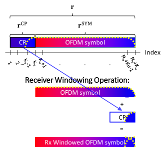
Figure 3: Indexing of $\mathbf{\bm{r}}$ and identification of its parts $\mathbf{\bm{r}}^{\text{CP}}$ and $\mathbf{\bm{r}}^{\text{SYM}}$ within a demonstration of how receiver windowing operation is performed.

$$\left(\mathbf{\bm{y}}_{l,u}\left[s\right]\mathbf{\bm{r}}_{m,l,u}\left[s\right]+\mathbf{\bm{y}}_{l,u}\left[s-N_{u}\right]\mathbf{\bm{r}}_{m,l,u}\left[s-N_{u}\right]\right)\tfrac{\exp\left(\jmath\tfrac{2\pi M_{u,m}\left(s-K_{u}-1\right)}{N_{u}}\right)}{\sqrt{N_{u}}}.$$ (29)

Accordingly, by removing the non-windowed contribution from all windowed samples and adding their respective windowed contribution to the FFT output, the SC symbol that is receiver windowed with window duration $0<r\leq K_{u}$ can be written as

$$\mathbf{\bm{Y}}_{u}\left[m,l,r\right]=\mathbf{\bm{Y}}_{u}\left[m,l,0\right]+\sum_{s=N_{u}+K_{u}-r+1}^{N_{u}+K_{u}}\left(\mathbf{\bm{y}}_{l,u}\left[s\right]\left(\mathbf{\bm{r}}_{m,l,u}\left[s\right]-1\right)+\mathbf{\bm{y}}_{l,u}\left[s-N_{u}\right]\mathbf{\bm{r}}_{m,l,u}\left[s-N_{u}\right]\right)\tfrac{\exp\left(\jmath\tfrac{2\pi M_{u,m}\left(s-K_{u}-1\right)}{N_{u}}\right)}{\sqrt{N_{u}}}.$$ (30)

Plugging $\mathbf{\bm{r}}_{m,l,u}\left[s\right]=1-\mathbf{\bm{r}}_{m,l,u}\left[s-N_{u}\right]$ for the windowed region per [12, 15], (LABEL:eq:rxwinsymlong) can be simplified to

$$\mathbf{\bm{Y}}_{u}\left[m,l,r\right]=\mathbf{\bm{Y}}_{u}\left[m,l,0\right]+\sum_{s=N_{u}+K_{u}-r+1}^{N_{u}+K_{u}}\left(\mathbf{\bm{y}}_{l,u}\left[s-N_{u}\right]-\mathbf{\bm{y}}_{l,u}\left[s\right]\right)\mathbf{\bm{r}}_{m,l,u}\left[s-N_{u}\right]\tfrac{\exp\left(\jmath\tfrac{2\pi M_{u,m}\left(s-K_{u}-1\right)}{N_{u}}\right)}{\sqrt{N_{u}}},$$ (31)

which allows computing the receiver windowed symbols with reduced computational complexity.

III-B2 Optimum Receiver Windowing Duration Estimation Algorithm

The optimum receiver windowing duration similarly maximizes (9). However, unlike the gNB that has predicted the CFR coefficients and already knows the payload, the UEs know neither. However, there are other higher order statistics that can be exploited by the UEs. Similar to (8), one can write

$$\mathbf{\bm{Y}}_{u}\left[m,l,r\right]=\mathbf{\bm{H}}_{u}\left[m,l\right]\left(\mathbf{\bm{D}}_{u}\left[m,l\right]+\mathbf{\bm{P}}_{u}\left[m,l\right]\right)+\tilde{\mathbf{\bm{N}}}_{u}\left[m,l,r\right]+\tilde{n}_{u}\left[m,l,r\right],$$ (32)

where $\mathbf{\bm{H}}_{u}\left[m,l\right]$ is the actual CFR coefficient affecting the $m$th subcarrier of $l$th OFDM symbol of $u$th user, $\tilde{\mathbf{\bm{N}}}_{u}\left[m,l,r\right]$ is the combined ACI, ICI and ISI affecting the aforementioned RE if receiver window duration $r$ is used, and $\tilde{n}_{u}\left[m,l,r\right]$ is the noise value affecting the aforementioned RE. Let the 2-tuple elements of the set $\mathbb{P}_{u}\left[\dot{m},\dot{l}\right]$ refer to the subcarrier and OFDM symbol indices of $P$ REs that are statistically expected to experience the channels most correlated with $\mathbf{\bm{H}}_{u}\left[\dot{m},\dot{l}\right]$[21]. To keep equations concise, we will only use $\mathbf{\bm{D}}_{u}\left[m,l\right]$ to refer to $\mathbf{\bm{D}}_{u}\left[m,l\right]+\mathbf{\bm{P}}_{u}\left[m,l\right]$ from this point onward. Even though no element other than $\mathbf{\bm{P}}_{u}\left[m,l\right]$ in the equation is known, the UE can still obtain

$$\breve{\mathbf{\bm{Y}}}_{u}\left[\dot{m},\dot{l},r\right]\coloneqq\operatorname{var}\left[\left\{\mathbf{\bm{Y}}_{u}\left[m,l,r\right],\left(m,l\right)\in\mathbb{P}_{u}\left[\dot{m},\dot{l}\right]\right\}\right]$$ (33)

$$=\operatorname{var}\left[\left\{\mathbf{\bm{H}}_{u}\left[m,l\right]\mathbf{\bm{D}}_{u}\left[m,l\right]+\tilde{\mathbf{\bm{N}}}_{u}\left[m,l,r\right]+\tilde{n}_{u}\left[m,l,r\right]\right\}\right]$$ (34)

$$=\operatorname{var}\left[\left\{\mathbf{\bm{H}}_{u}\left[m,l\right]\mathbf{\bm{D}}_{u}\left[m,l\right]\right\}\right]+\operatorname{var}\left[\left\{\tilde{n}_{u}\left[m,l,r\right]\right\}\right]+\operatorname{var}\left[\left\{\tilde{\mathbf{\bm{N}}}_{u}\left[m,l,r\right]\right\}\right],$$ (35)

where the set definitions $\left(m,l\right)\in\mathbb{P}_{u}\left[\dot{m},\dot{l}\right]$ were removed after the first line to keep equations concise, but are always implied throughout the rest of this section for all mean and variance operations, and an equal-weight variance is assumed, or in probability terms, all elements are assigned the same $1/P$ probability. Weighting elements with the correlation between $\mathbf{\bm{H}}_{u}\left[m,l\right]$ and $\mathbf{\bm{H}}_{u}\left[\dot{m},\dot{l}\right]$[22] is optimum[23], however, the equiweight implementation drastically reduces the computational complexity as will be shown below, without an observable performance loss. Note that since $\tilde{n}_{u}\left[m,l,r\right]\sim\mathcal{CN}\left(0,1\right)\forall u,m,l,r$, although the noise value itself changes with windowing, the noise variance remains unity. Furhermore, as ICI and ISI are separated, the variance in the actual channel coefficients can be assumed to remain constant regardless of window duration as well. Thus, the CFR coefficient, transmitted data and noise variance remain constant regardless of applied window, but the combined interference and its variance varies with the windowing operation. Although it is impossible to distinguish between these components by looking at the effects of windowing on a single received symbol, the spectrotemporal correlation of channel and interference can be exploited to identify the amount of combined interference in a group of REs. That is, although $\operatorname{var}\left[\left\{\tilde{\mathbf{\bm{N}}}_{u}\left[m,l,r\right],\left(m,l\right)\in\mathbb{P}_{u}\left[\dot{m},\dot{l}\right]\right\}\right]$ can not be found explicitly, one can conclude that

$$\operatorname*{\arg\,\min}_{r}\breve{\mathbf{\bm{Y}}}_{u}\left[\dot{m},\dot{l},r\right]\triangleq\operatorname*{\arg\,\min}_{r}\operatorname{var}\left[\left\{\tilde{\mathbf{\bm{N}}}_{u}\left[m,l,r\right]\right\}\right].$$ (36)

The optimum receiver windowing duration calculation algorithm utilizes (36) to minimize the combined interference energy and maximize capacity. With similar reasoning to Algorithm 1, Algorithm 2 also starts with the assumption of zero initial window duration, and checks to see whether longer window durations are beneficial for each RE. Let us now investigate a possible reduced complexity implementation of this idea, particularly utilizing the relation between $\mathbf{\bm{Y}}_{u}\left[m,l,0\right]$ and $\mathbf{\bm{Y}}_{u}\left[m,l,r\right]$ as shown in (LABEL:eq:rxwinsymlong). Let us first define

1: 

2:Algorithm 2: Estimate $\mathbf{\bm{R}}_{u}$ & $\hat{\mathbf{\bm{Y}}}_{u}$

3: 

4:$\mathbf{\bm{R}}_{u}\leftarrow 0$

5:for all $m\in M_{u},l\in L_{u}$ do

6:     $\breve{\mathbf{\bm{Y}}}_{u}\left[m,l,0\right]\leftarrow\textup{(\ref{eq:rxsymvariancedef})}$

7:     for $r\leftarrow 1,K_{u}$ do

8:         $\breve{\mathbf{\bm{Y}}}_{u}\left[m,l,r\right]\leftarrow\textup{(\ref{eq:rxwinvariance})}$

9:         if $\breve{\mathbf{\bm{Y}}}_{u}\left[m,l,r\right]>\breve{\mathbf{\bm{Y}}}_{u}\left[m,l,r-1\right]$ then

10:              $\mathbf{\bm{R}}_{u}\left[m,l\right]\leftarrow r-1$

11:              break

12:         end if

13:     end for

14:     $\hat{\mathbf{\bm{Y}}}_{u}\left[m,l\right]\leftarrow\textup{(\ref{eq:rxwinsym})}$

15:end for

$$\ddot{y}_{u}\left[m,l,r\right]=\mathbf{\bm{Y}}_{u}\left[m,l,r\right]-\mathbf{\bm{Y}}_{u}\left[m,l,0\right]$$ (37)

$$=\sum_{s=N_{u}+K_{u}-r+1}^{N_{u}+K_{u}}\left(\mathbf{\bm{y}}_{l,u}\left[s-N_{u}\right]-\mathbf{\bm{y}}_{l,u}\left[s\right]\right)\mathbf{\bm{r}}_{m,l,u}\left[s-N_{u}\right]\tfrac{\exp\left(\jmath\tfrac{2\pi M_{u,m}\left(s-K_{u}-1\right)}{N_{u}}\right)}{\sqrt{N_{u}}}$$ (38)

to keep following equations concise. Then

$$\breve{\mathbf{\bm{Y}}}_{u}\left[\dot{m},\dot{l},r\right]=\sum_{\left(m,l\right)\in\mathbb{P}_{u}\left[\dot{m},\dot{l}\right]}\frac{\left|\mathbf{\bm{Y}}_{u}\left[m,l,r\right]-\sum_{\left(\ddot{m},\ddot{l}\right)\in\mathbb{P}_{u}\left[\dot{m},\dot{l}\right]}\mathbf{\bm{Y}}_{u}\left[\dot{m},\dot{l},r\right]/P\right|^{2}}{P}$$ (39)

$$=\frac{1}{P^{3}}\sum_{\left(m,l\right)\in\mathbb{P}_{u}\left[\dot{m},\dot{l}\right]}\left|\mathbf{\bm{Y}}_{u}\left[m,l,r\right]\left(P-1\right)-\sum_{\left(\ddot{m},\ddot{l}\right)\in\mathbb{P}_{u}\left[\dot{m},\dot{l}\right]\setminus\left(m,l\right)}\mathbf{\bm{Y}}_{u}\left[\ddot{m},\ddot{l},r\right]\right|^{2}$$ (40)

$$=\frac{1}{P^{3}}\sum_{\left(m,l\right)\in\mathbb{P}_{u}\left[\dot{m},\dot{l}\right]}\left|\mathbf{\bm{Y}}_{u}\left[m,l,0\right]\left(P-1\right)-\sum_{\left(\ddot{m},\ddot{l}\right)\in\mathbb{P}_{u}\left[\dot{m},\dot{l}\right]\setminus\left(m,l\right)}\mathbf{\bm{Y}}_{u}\left[\ddot{m},\ddot{l},0\right]+\ddot{y}_{u}\left[m,l,r\right]\left(P-1\right)-\sum_{\left(\ddot{m},\ddot{l}\right)\in\mathbb{P}_{u}\left[\dot{m},\dot{l}\right]\setminus\left(m,l\right)}\ddot{y}_{u}\left[\ddot{m},\ddot{l},r\right]\right|^{2}$$ (41)

demonstrates that once

$$\mathbf{\bm{Y}}_{u}\left[m,l,0\right]\left(P-1\right)-\sum_{\left(\ddot{m},\ddot{l}\right)\in\mathbb{P}_{u}\left[\dot{m},\dot{l}\right]\setminus\left(m,l\right)}\mathbf{\bm{Y}}_{u}\left[\ddot{m},\ddot{l},0\right]$$ (42)

is calculated, the variance of the windowed cases can be calculated by adding the window differences and summing the squared magnitudes. The advantage of the equiweight assumption becomes clear at this point, a simple investigation reveals that once $\breve{\mathbf{\bm{Y}}}_{u}\left[\dot{m},\dot{l},r\right]$ is calculated for an RE, the same calculation for neighboring REs only require adding and removing contributions from few REs. More information on computational complexity is provided in Section III-B3.

III-B3 Computational Complexity

Calculating (42) for $\left(m,l\right)\leftarrow\left(m_{1},l_{1}\right)\in\mathbb{P}_{u}\left[\dot{m},\dot{l}\right]$ for a single RE requires $2P$ real additions and $2$ real multiplications. The result of the same equation for another RE with indices $\left(m,l\right)\leftarrow\left(m_{2},l_{2}\right)\in\mathbb{P}_{u}\left[\dot{m},\dot{l}\right]$ can be obtained by adding $P\left(\mathbf{\bm{Y}}_{u}\left[m_{2},l_{2},0\right]-\mathbf{\bm{Y}}_{u}\left[m_{1},l_{1},0\right]\right)$ to the previously calculated value, resulting in $4$ real additions and $2$ real multiplications. Thus, calculating (42) $\forall\left(m,l\right)\in\mathbb{P}_{u}\left[\dot{m},\dot{l}\right]$ requires a total of $6P-4$ real additions and $2P$ real multiplications.

Trials show that the subsets $\mathbb{P}_{u}\left[\dot{m},\dot{l}\right]$ differ at most by $\log\left(c+P\right)$ individual REs for neighbor REs under vehicular channels[24] for statistically meaningful $P$ values, where $c$ is a small positive constant. While the mean subset difference is well below that for the possible transmission time interval (TTI) durations and bandwidth part configurations in NR, $\log\left(P\right)$ will be assumed for all REs as the mean asymptotically reaches this number with increasing number of allocated slots and resource blocks, and to mitigate $c$. Thus, after (42) is calculated for an RE for $\mathbb{P}_{u}\left[\dot{m}_{1},\dot{l}_{1}\right]$, the results can be generalized for the same RE for another $\mathbb{P}_{u}\left[\dot{m}_{2},\dot{l}_{2}\right],\left(\dot{m}_{2},\dot{l}_{2}\right)\leftarrow\exists\left\{\left(\dot{m}_{1}\pm 1,\dot{l}_{1}\right),\left(\dot{m}_{1},\dot{l}_{1}\pm 1\right)\right\}$ by adding $P\left(\sum_{\left(\ddot{m},\ddot{l}\right)\in\mathbb{P}_{u}\left[\dot{m}_{2},\dot{l}_{2}\right]}\mathbf{\bm{Y}}_{u}\left[\ddot{m},\ddot{l},0\right]-\sum_{\left(\ddot{m},\ddot{l}\right)\in\mathbb{P}_{u}\left[\dot{m}_{1},\dot{l}_{1}\right]}\mathbf{\bm{Y}}_{u}\left[\ddot{m},\ddot{l},0\right]\right)$ to the previous findings, which requires $4\log\left(P\right)$ real additions and $2$ real multiplications. The findings can then similarly propagate to other REs $\in\mathbb{P}_{u}\left[\dot{m}_{2},\dot{l}_{2}\right]$ by performing $4$ real additions and $2$ real multiplications each as described above. Therefore, number of operations required to obtain (42) $\forall\left(m,l\right),\forall\left(\dot{m},\dot{l}\right)$ is upper bounded by $4\left(M_{u}L_{u}\left(P+\log\left(P\right)-1\right)-\log\left(P\right)\right)+2P$ real additions and $2PM_{u}L_{u}$ real multiplications.

A direct investigation reveals that each (38) calculation requires $6r-2$ real additions and $6r$ real multiplications to obtain the symbol windowed with window duration $r$. Once the relevant (38) values are calculated, the number of equations required to calculate the difference $\ddot{y}_{u}\left[m,l,r\right]\left(P-1\right)-\sum_{\left(\ddot{m},\ddot{l}\right)\in\mathbb{P}_{u}\left[\dot{m},\dot{l}\right]\setminus\left(m,l\right)}\ddot{y}_{u}\left[\ddot{m},\ddot{l},r\right]$ in (41) is the same as the number of operations required to obtain (42). It should be noted that these values are only required for $\left(m,l\right)\in\mathbb{P}_{u}\left[\dot{m},\dot{l}\right]$ if $\breve{\mathbf{\bm{Y}}}_{u}\left[\dot{m},\dot{l},r\right]$ is being calculated, which is not always needed.

After both differences in (41) is obtained, the sum of the squared magnitudes of the sum of differences can be calculated to finalize (41) calculation. This requires $3P-1$ real additions and $2P$ real multiplications. If $\mathbf{\bm{R}}_{u}\left[m,l\right]=R$, (41) must be calculated $\forall r\in\mathbb{N}_{\leq\min\left(R+1,K_{u}\right)}^{*}$. Once $\mathbf{\bm{R}}_{u}$ is found, (LABEL:eq:rxwinsym) is performed to obtain windowed symbols to continue reception, which requires only $2\#\left\{\mathbf{\bm{R}}_{u}\neq 0\right\}$ real additions and no multiplications. Some statistics for $\mathbf{\bm{R}}_{u}$ and number of operations performed for vehicular channel conditions are provided in Section IV. It should also be noted that the worst case time complexity of the described efficient implementation is on the order of $\mathcal{O}\left(K_{u}^{2}PM_{u}L_{u}\right)$, while a more straightforward operation count- and memory-wise exhaustive implementation can run within $\mathcal{O}\left(P+K_{u}\right)$.

III-C Further Notes on Computational Complexity

The algorithms presented in Section III are computationally tailored around the basic assumption that both transmitter and receiver window durations are expected to be short as the utilized extension was solely intended for the channel. While Section IV shows that this assumption holds, there are also other characteristics that can be exploited, such as the spectrotemporal correlation of window durations, and a non-obvious but comprehensible peak in the statistical receiver window duration probability distribution, all of which are presented and discussed in Section IV. This section was aimed to describe the basic ideas and only simple, universal algorithmic implementation specific details in the most comprehensible manner. Further possible reductions in computational complexity are mentioned along with numerical findings in Section IV.

IV Numerical Verification

Although the proposed method is formulated for networks with any number of UEs, in this work, a simple network limited to a base station (BS) and two UEs equally sharing a $7.68\text{\,}\mathrm{MHz}$ system bandwidth is considered for the sake of simplicity, as done in other similar works such as [25]. This also allows clearer presentation of the results. This network is realized numerous times with independent and random user data and instantaneous channels, and all presented results are the arithmetic means of all realizations unless otherwise specified. The parameters provided in [26] for link level waveform evaluation under $6\text{\,}\mathrm{GHz}$ were used when possible. One of the UEs is a high mobility node experiencing a channel that has $30\text{\,}\mathrm{ns}$ RMS delay spread and $120\text{\,}\mathrm{km}\text{/}\mathrm{h}$ mobility, hereinafter referred to as the “’f’ast user”, communicating using 60 subcarriers of an OFDM numerology with subcarrier spacing of $\Delta_{f_{f}}=$60\text{\,}\mathrm{kHz}$$. The second UEs is a moderate mobility node experiencing a channel that has $100\text{\,}\mathrm{ns}$ RMS delay spread and $30\text{\,}\mathrm{km}\text{/}\mathrm{h}$ mobility, hereinafter referred to as the “’s’low user”, communicating using 120 subcarriers of the $\Delta_{f_{s}}=$30\text{\,}\mathrm{kHz}$$ numerology in the adjacent band. The PDP of fast user’s channel is 3GPP tapped delay line (TDL)-A[24] in $\nicefrac{{1}}{{2}}$, TDL-B in $\nicefrac{{1}}{{3}}$ and TDL-C in $\nicefrac{{1}}{{6}}$ of the simulations to demonstrate the operability of the algorithm under different channel models. Similarly, the PDP of slow user’s channel is 3GPP TDL-B in $\nicefrac{{1}}{{2}}$, and TDL-A or TDL-C each in $\nicefrac{{1}}{{4}}$ of the simulations. The Doppler spectra of both channels are assumed to be classical Jakes [27] at all times[24]. There is a $240\text{\,}\mathrm{kHz}$ guard band between users. The SNR of each user is sweeped from $5\text{\,}\mathrm{dB}15\text{\,}\mathrm{dB}$ during which the SNR of the other user is fixed to $10\text{\,}\mathrm{dB}$.

Results are obtained for a duration of one NR format 4 slot[28] in the slow user’s reference, where both flexible symbols are utilized for UL. The UL transmission interval of a slot followed by the DL transmission interval of the consecutive slot is investigated. There’s a timing offset of 64 samples in the UL, whereas the consequent DL period is synchronous. The UL DMRS received at the gNB, which are physical uplink shared channel (PUSCH) DMRS type B mapped[29], are used to estimate the channel. Only this time invariant estimate is used in Algorithm 2 for the following DL transmission interval. This presents the worst-case performance of especially Algorithm 2 under minimum available information. The rate of performance improvement for increasing number of consecutive slots with the help of channel prediction[18] is left for future work. The DL DMRS configuration is single port single layer mapped with crucial parameters uniquely defining the mapping dmrs-AdditionalPosition 3 and dmrs-TypeA-Position pos2[29]. No windowing or power control is applied to UL signals as well, reducing the performance of solely the proposed methods making it the worst case scenario.

Unless otherwise specified, both UEs utilize a normal CP overhead of $\nicefrac{{9}}{{128}}$ with no additional extension for windowing at all times, thus conserving standard 5G NR symbol structure. For comparison, optimum fixed extension windowing algorithm[12] is also featured utilizing the standard extended CP overhead of 25% and the additional extension is used for either transmitter or receiver windowing, as well as filtered- (F-OFDM)[30, 31] and $N$-Continuous (NC-OFDM)[32], the tone offset for the former, in accord with the resource allocation, being 7.5 and 3.5 tones for the slow and fast user, respectively; and the $N$ parameter for the latter being $N_{\text{fast}}=1$ and $N_{\text{slow}}=2$ per the original work, and both receivers use the iterative correcting receiver[32, Sec. 3] performing 8 iterations. Link adaptation is omitted in the system, all RBs are assigned the same constant MCS which consists of QPSK modulation and $\left(21/32\right)\times\left(7/15\right)$ standard[33, 34] and extended[35] Bose–Chaudhuri–Hocquenghem (BCH) Turbo product code [36] for the slow user and $\left(7/16\right)\times\left(7/15\right)$ for the fast user at all times. The MCSs are chosen such that both users operate slightly below the target bit-error rate (BER) at the minimum SNR, thus the SNR difference between the users can be referred to as the excess SNR for the utilized SNR values. $P\leftarrow 33$ for both users in Algorithm 2 so that a meaningful z-test can be performed.

The OOB emission of investigated waveforms are depicted in Fig. 4, where the lines denoted with $\Delta\gamma$ is the results for Algorithm 1, for which the windowed user’s average SNR is greater than that of the victim by the provided value; and the sampling points of the victim subcarriers are marked to distinguish between modulations and to provide means to understand the unorthodox frequency localization characteristics of F-OFDM[31] and optimum fixed extension transmitter windowing (ETW) algorithm[12] to unfamiliar readers. Both F-OFDM and ETW-OFDM have unmatched interference performance in the victim’s band, but F-OFDM requires the receiver to perform matched filtering, and ETW-OFDM requires an extension that may disturb the standard frame structure, or reduced throughput if the standard extensions are used in vehicular channels as seen in Table II. The interference performance of NC-OFDM at the edge subcarriers also outperforms all cases of Algorithm 1, but Algorithm 1 takes over in the band center subcarriers for high excess SNR. Furthermore, NC-OFDM also requires receiver-side operations, thus has no advantage over F-OFDM. It is seen that while Algorithm 1 has little advantage if the windowing user has no excess SNR, the level of interference decreases further as the window duration is able to increase when the user has excess SNR. Although the proposed algorithm uses the same window design used in ETW-OFDM, the fact that not all REs are windowed prevents the same localization from surfacing. It should also be noted that the gains are a significant function of channel responses of both UEs, and the transmit OOB emission is unable to demonstrate the gains clearly.

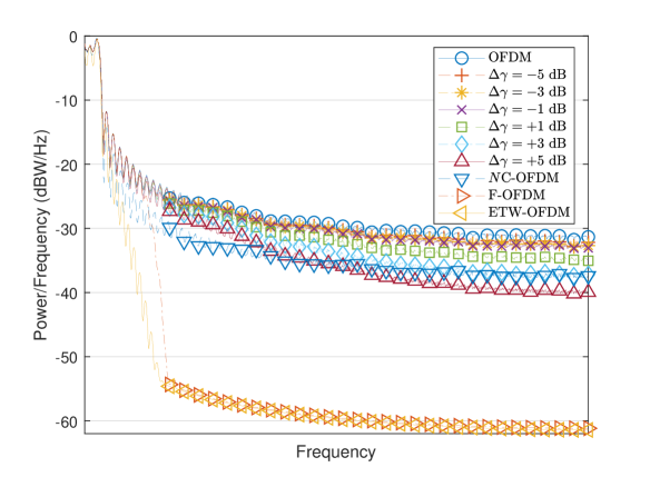
Figure 4: OOB emission of investigated modulations.

The fair proportional network throughput, calculated similar to network proportional network capacity using the geometric means of throughput of each user, can be seen in Table II for optimum fixed extension transmitter and receiver windowed OFDM[12], NC-OFDM, conventional CP-OFDM, adaptive transmitter windowed with estimates obtained using Algorithm 1, adaptive transmitter windowed with optimum durations, F-OFDM, adaptive receiver windowed using durations calculated using Algorithm 2, adaptive transmitter and receiver windowed with transmitter windowing durations calculated using Algorithm 1 without knowing receivers are applying Algorithm 2 followed by Algorithm 2 at the receivers, Algorithm 2 applied to the signals that are adaptive transmitter windowed with optimum durations, adaptive transmitter and receiver windowed with transmitter windowing durations calculated using Algorithm 1 knowing receivers are applying Algorithm 2 followed by Algorithm 2 at the receivers, and adaptive transmitter and receiver windowed with durations optimized jointly. The optimum values were obtained by maximizing the fair proportional network throughput using an evolutionary integer genetic algorithm[37] to find the optimum inputs to Algorithms 1 and/or 2 under actual time-varying channels. It can be seen that although previously proposed extended windowing algorithms improve the BERs, increasing the effective symbol duration by ~18% erases the positive implications on the throughput and reduces it. The artificial noise introduced by the NC-OFDM cannot be resolved at the receivers at these high mobility conditions correctly yielding a decrease in actual throughput. It can be seen that even the featured worst case results of the proposed algorithms increase the throughput and improving algorithm outputs by channel prediction promises further gains closer to optimum. While F-OFDM provides higher throughput compared to Algorithm 1 and adaptive transmitter windowing, it requires that both ends of the communication are aware of the filtering process and apply it[38, 30, 31]. Although knowledge of such improves the throughput, the proposed algorithms do not require the knowledge and action of the counterpart and this is the strength of the proposed method compared to F-OFDM.

TABLE II: Fair proportional network throughput of tested modulations

Modulation	Throughput (Mbps)	Gain over CP-OFDM
ETW-OFDM	1.1949	-15.832%
ERW-OFDM	1.1952	-15.708%
$N$C-OFDM	1.3927	-1.456%
CP-OFDM	1.3985	-
Algorithm 1	1.3986	+0.042%
TW-OFDM (w/o Ext)	1.3987	+0.049%
F-OFDM	1.3988	+0.057%
Algorithm 2	1.3990	+0.071%
Algorithm 1 + Algorithm 2 (independent)	1.3991	+0.078%
TW-OFDM + Algorithm 2 (independent)	1.3992	+0.085%
Algorithm 1 + Algorithm 2 (joint)	1.3996	+0.114%
TW-OFDM+ RW-OFDM (joint)	1.3998	+0.128%

To show the dependence of window durations on excess SNR, the ratio of estimated and optimum expected window durations to the CP of the corresponding UEs as a function of the SNR difference between the user in interest and the other user are demonstrated in Fig. 5. The results are ordered as follows: Receiver windowing durations of only Algorithm 2, Algorithm 2 applied to the signals transmitted after applying Algorithm 1, Algorithm 2 applied to transmitter windowed samples with the optimum duration if the gNB is unaware that receivers employ Algorithm 2, Algorithm 2 applied to to the signals produced Algorithm 1 where gNB knows both receivers also employ Algorithm 2, and Algorithm 2 applied to transmitter windowed samples with the optimum duration calculated knowing that receiver will apply Algorithm 2; as well as transmitter windowing durations estimated by Algorithm 1, optimum adaptive transmitter windowing durations, transmitter windowing duration estimates provided by Algorithm 1 knowing that both receivers also employ Algorithm 2 and optimum transmitter windowing durations calculated if both receivers also employ Algorithm 2. A critical observation is that the transmitter windowing durations, both estimated and actual optimum, increase as the SNR of the user increases, whereas the receiver windowing duration decreases. This proves the basic idea behind fair optimization that the ones with excess SNR must focus on their impact on others whereas the ones with lesser SNR must focus on the impact they receive from others. It can also be seen that the optimum durations for each side get shorter once the resources are jointly used, i.e., the gNB knows that receivers utilize Algorithm 2.

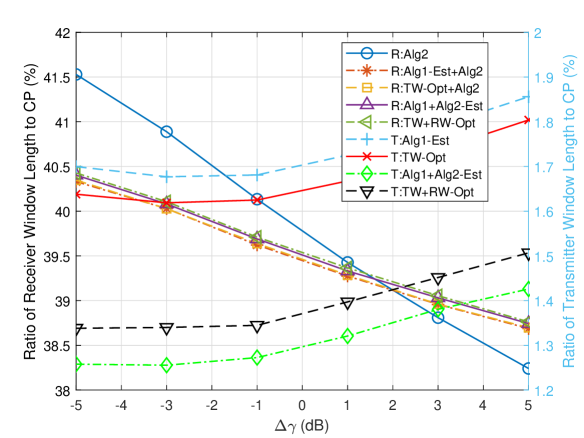
Figure 5: $\mathbb{E}\left\{\mathbf{\bm{R}}_{u}/K_{u}\right\}$ and $\mathbb{E}\left\{\mathbf{\bm{T}}_{u}/K_{u}\right\}$ against the SNR difference between users.

Fig. 6 shows the probability of the calculated window duration being a certain amount away from the optimum duration, between Algorithm 1 and optimum transmitter windowing durations, between Algorithm 1 calculated knowing that receivers utilize Algorithm 2 and optimum transmitter window durations obtained when receivers employ Algorithm 2; and receiver windowing durations estimated at the transmitter during calculation of Algorithm 2 and the values obtained at receivers. It can be seen that the guess for both the transmitter and the receiver windowing durations are more accurate for the slower user, proving the dependence on mobility at estimates without channel tracking and prediction. Furthermore, since receiver windowing durations only matter for the RBs in interest as discussed before, receiver windowing durations can be guessed with over 98% probability without making an error. The transmitter windowing estimates have more than 95% probability of being the same as optimum, while overestimating is slightly more probable in the only Algorithm 1 case while underestimating is more probable in the both algorithms utilized case.

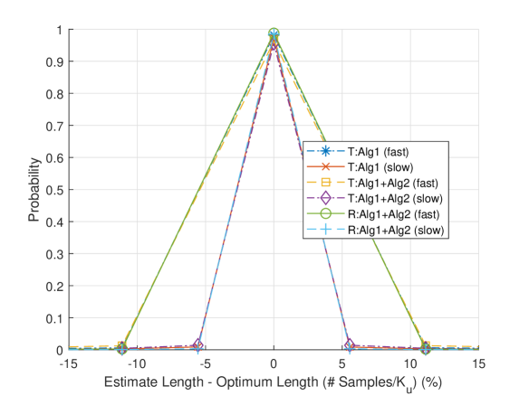
Figure 6: Probability of the error between estimated and optimum window lengths being equal to certain percentages of CP.

Fig. 7 and Fig. 8 show the amount of receiver and transmitter windowing applied at the band centers and edges and checks the validity of [13] where the window durations are labeled similar to that of Fig. 5. It can be seen that the amount of transmitter windowing indeed increases at the band edges, and furthermore it is more important that the faster user with the larger subcarrier spacing and less spectral localization to apply more transmitter windowing. This derives from the fact that the power spectral density (PSD) of signals with larger subcarrier spacing decay slower than those with smaller subcarrier spacing, hence are more crucial for the interference in the system. It can be seen that the receiver windowing durations are higher at the band centers and higher for the user with lower subcarrier spacing. This occurs partly due to the window function design. The window functions are designed to minimize the absorption outside the the band of interest, however as the pass-band of the window gets smaller, the reduction performance decreases as well[12]. Since the window pass-bands are smaller on the edge subcarriers, the gain from reduced ACI and ICI reduces whereas the performance reduction due to increased ISI stays the same. This favors longer window durations at the inner subcarriers where increasing window durations result in significant ICI and ACI reduction. The gain from ICI reduction becomes more prominent for the faster user which observes even higher window lengths at inner subcarriers due to the increased ICI. The gain from either type of windowing reduces for both users as windowing at the counterparty is introduced to the systems, both by reduction of forces driving windowing at a given side and also increase in ISI occurring by applying windowing, as both users observe shorter windowing durations on either side that is more uniformly distributed from band centers to edges.

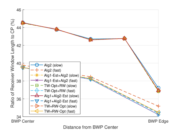
Figure 7: Receiver windowing durations as a function of distance from center of the consumed band.

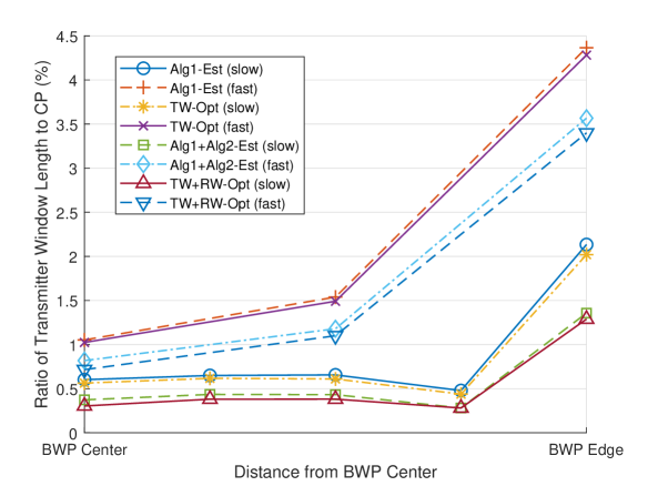
Figure 8: Transmitter windowing durations as a function of distance from center of the consumed band.

Before the average number of performed operations are provided for presented Algorithms in their current forms and compared, spectrotemporal statistics of window durations are provided to demonstrate that there is room for further computational complexity reductions, which are left for future works. Both experienced channel and amount of interference are highly correlated in both dimensions, which in turn create correlated window durations that can reduce complexity load. For example, Fig. 9 shows the probability that window durations calculated for adjacent subcarriers differ by a given duration, as a function of CP length. It is seen that no more than $35\%$ CP duration difference occurred at any time. This suggests that if a subcarrier was calculated to have a long window duration, checking brief window durations for the adjacent subcarriers may be skipped at first and the search can start from a higher value. Furthermore, REs may be grouped and processed together. Fig. 10 presents the same results for Algorithm 2, showing that the differences are even smaller in both time and frequency as the duration is determined using the variance over a group of REs and the RE groups of adjacent RE differ little. It is also worth noting that window durations in adjacent REs of the faster user are more likely to differ by longer durations than that of the slower user, which depends on both increased subcarrier spacing and channel variations.

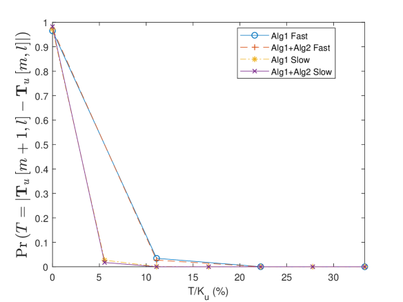
Figure 9: Probability that transmitter window durations in adjacent subcarriers differ by the given amount.

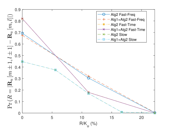
Figure 10: Probability that receiver window durations in adjacent REs differ by the given amount.

Finally, the computational load of the algorithms in their presented forms is analyzed and compared with F-OFDM. The filter lengths are $N_{u}/2+1$ per [31], and since filters consist of complex values, the computational complexity of F-OFDM is $\left(N_{u}+K_{u}\right)L_{u}\left(3N_{u}/2+2\right)$ real additions and $\left(N_{u}+K_{u}\right)L_{u}\left(2N_{u}+4\right)$ real multiplications at the UE, and these values summed over all users at the gNB. The computational complexities of the presented algorithms depend on the window duration and side of each RE, of which values have the probability distributions shown in Fig. 11. Accordingly, the gNB and UE side computational complexities of the algorithms are presented in Table III. As Algorithm 1 only runs at the gNB and Algorithm 2 only runs at the UE without any operation requirements at the counterpart, the counterpart complexities are 0 for both users. It is seen that while the gNB side complexity for Algorithm 1 is higher than that of F-OFDM, assumin that gNBs are not computationally bounded, the transparency of Algorithm 1 still makes it a possible candidate under heavy traffic. The computational complexity of Algorithm 2 is similar to that of F-OFDM if the further computational complexity reduction tricks described in the preceding paragraph are not employed, and Algorithm 2 is also transparent to the transmitter. Another interesting observation that can be made from Fig. 11 is that for Algorithm 2, under severe ACI conditions, longer window durations may be beneficial, however since the window duration is limited by CP length, all those results manifest themselves at the upper bound, creating a high probability peak at the longest duration. Computational complexity can be further reduced if Algorithm 2 is modified to check the longest possibility before others, however these highly implementation specific details are left for future work.

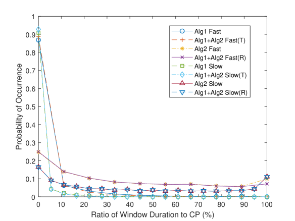
Figure 11: Probability of transmitter (T) and receiver (R) window durations occurring in test scenarios.

TABLE III: Computational Complexities of F-OFDM and Algorithms 1 and 2

Algorithm	gNB add	gNB mult	UE add	UE mult
F-OFDM	1907040	2551488	637872+ 1269168	854880+ 1696608
Alg. 1	5342353	5332295	0	0
Alg. 2	0	0	2088692+ 4166143	1054709+ 2236623

V Conclusion

In this work, we have demonstrated the concept of frame structure compliant computationally efficient adaptive per-RE extensionless transmitter windowing to maximize fair proportional beyond 5G network capacity in the DL, and universal per-RE receiver windowing that requires no additional knowledge. Results demonstrate that gains are possible from windowing without introducing extra extensions that defy the frame structure if the side, RE and duration to apply windowing is calculated carefully. The user with higher excess SNR must apply longer transmitter windowing as they can resist the SNR reduction, whereas the user with lower excess SNR must apply longer receiver windowing. Users with higher subcarrier spacing and higher mobility cause more interference in the system hence should apply more transmitter windowing, whereas users with lower subcarrier spacing must focus on receiver windowing. Optimum transmitter window durations are longer at the edges whereas optimum receiver window durations are longer at band centers. Emulating the multipath multiple access channel allows the gNB to estimate optimum transmitter windowing durations prior to transmission with $95\%$ confidence. Using the variance of received symbols allows the UEs to calculate optimal receiver windowing durations without calculations requiring further knowledge about the network and channel. While both algorithms are presented for per-RE calculations, spectrotemporal correlation of window durations allow reduced computational complexity implementations than those described. Extensionless windowing at either side does not require action and information transfer to the communication counterpart and is fully compatible with previous and current generations, however the knowledge of adaptive windowing applied at the counterpart allows joint optimization that reveals higher gains.

Berker Peköz (GS’15) received the B.S. degree in electrical and electronics engineering from Middle East Technical University, Ankara, Turkey in 2015, and the M.S.E.E. from University of South Florida, Tampa, FL, USA in 2017. He was a Co-op Intern at the Space Division of Turkish Aerospace Industries, Inc., Ankara, Turkey in 2013, and a Summer Intern at the Laboratory for High Performance DSP & Network Computing Research, New Jersey Institute of Technology, Newark, NJ, USA in 2014. He is currently pursuing the Ph.D. at University of South Florida, Tampa, FL, USA. His research is concerned with standard compliant waveform design and processing. Mr. Peköz is a member of Tau Beta Pi.

Selçuk Köse (S’10–M’12) received the B.S. degree in electrical and electronics engineering from Bilkent University, Ankara, Turkey, in 2006, and the M.S. and Ph.D. degrees in electrical engineering from the University of Rochester, Rochester, NY, USA, in 2008 and 2012, respectively. He was a Member of the VLSI Design Center at Scientific and Technological Research Council (TÜBİTAK), Ankara, Turkey; the Central Technology and Special Circuits Team of Enterprise Microprocessor Division at Intel Corporation, Santa Clara, CA, USA; and the RF, Analog, and Sensor Group at Freescale Semiconductor, Tempe, AZ, USA. He was an Assistant Professor of Electrical Engineering at the University of South Florida, Tampa, FL, USA. He is currently an Associate Professor of Electrical Engineering at the University of Rochester, Rochester, NY, USA. His current research interests include integrated voltage regulation, 3-D integration, hardware security, and green computing. Dr. Köse was a recipient of the NSF CAREER Award, the Cisco Research Award, the USF College of Engineering Outstanding Junior Researcher Award, and the USF Outstanding Faculty Award. He is an Associate Editor of the World Scientific Journal of Circuits, Systems, and Computers and the Elsevier Microelectronics Journal. He has served on the Technical Program and Organization Committees of various conferences.

Hüseyin Arslan (S’95-M’98-SM’04-F’15) received the B.S. degree in electrical and electronics engineering from Middle East Technical University, Ankara, Turkey in 1992, and the M.S. and Ph.D. degrees in electrical engineering from Southern Methodist University, Dallas, TX, USA in 1994 and 1998, respectively. From January 1998 to August 2002, he was with the research group of Ericsson Inc., Charlotte, NC, USA, where he was involved with several projects related to 2G and 3G wireless communication systems. He has worked as part time consultant for various companies and institutions including Anritsu Company (Morgan Hill, CA, USA), The Scientific and Technological Research Council of Turkey (TÜBİTAK). He is currently a Professor of Electrical Engineering at the University of South Florida, Tampa, FL, USA, and the Dean of the College of Engineering and Natural Sciences at the İstanbul Medipol University, İstanbul, Turkey. Dr. Arslan’s research interests are related to advanced signal processing techniques at the physical and medium access layers, with cross-layer design for networking adaptivity and Quality of Service (QoS) control. He has served as technical program committee chair, technical program committee member, session and symposium organizer, and workshop chair in several IEEE conferences. He is currently a member of the editorial board for the IEEE Communications Surveys and Tutorials and the Sensors Journal. He has also served as a member of the editorial board for the IEEE Transactions on Communications, the IEEE Transactions on Cognitive Communications and Networking (TCCN), the Elsevier Physical Communication Journal, the Hindawi Journal of Electrical and Computer Engineering, and Wiley Wireless Communication and Mobile Computing Journal.

References

- [1] D. Astely, E. Dahlman, A. Furuskär, Y. Jading, M. Lindström, and S. Parkvall, “LTE: the evolution of mobile broadband,” IEEE Commun. Mag., vol. 47, no. 4, pp. 44–51, Apr. 2009.
- [2] J. Andrews, S. Buzzi, W. Choi, S. Hanly, A. Lozano, A. Soong, and J. Zhang, “What will 5G be?” IEEE J. Sel. Areas Commun., vol. 32, no. 6, pp. 1065–1082, Jun. 2014.
- [3] R. W. Chang, “Synthesis of band-limited orthogonal signals for multichannel data transmission,” Bell Syst. Tech. J., vol. 45, no. 10, pp. 1775–1796, Dec. 1966.
- [4] S. Chen and J. Zhao, “The requirements, challenges, and technologies for 5G of terrestrial mobile telecommunication,” IEEE Commun. Mag., vol. 52, no. 5, pp. 36–43, May 2014.
- [5] Z. Ankaralı, B. Peköz, and H. Arslan, “Flexible radio access beyond 5G: A future projection on waveform, numerology & frame design principles,” IEEE Access, vol. 5, no. 1, pp. 18 295–18 309, Dec. 2017.
- [6] 3GPP, “NR; Physical layer procedures for data,” 3rd Generation Partnership Project (3GPP), Technical Specification (TS) 38.214, 01 2018, version 15.0.0.
- [7] R. Lupas and S. Verdu, “Near-far resistance of multiuser detectors in asynchronous channels,” IEEE Trans. Commun., vol. 38, no. 4, pp. 496–508, Apr. 1990.
- [8] X. Zhang, L. Zhang, P. Xiao, D. Ma, J. Wei, and Y. Xin, “Mixed numerologies interference analysis and inter-numerology interference cancellation for windowed OFDM systems,” IEEE Trans. Veh. Technol., vol. 67, no. 8, pp. 7047–7061, Aug. 2018.
- [9] 3GPP, “NR; Physical layer; General description,” 3rd Generation Partnership Project (3GPP), Technical Specification (TS) 38.201, 01 2018, version 15.0.0.
- [10] M. Gudmundson and P. O. Anderson, “Adjacent channel interference in an OFDM system,” in Proc. 1996 IEEE Veh. Technol. Conf., vol. 2, Atlanta, GA, Apr. 1996, pp. 918–922.
- [11] C. Muschallik, “Improving an OFDM reception using an adaptive Nyquist windowing,” IEEE Trans. Consum. Electron., vol. 42, no. 3, pp. 259–269, Aug. 1996.
- [12] E. Güvenkaya, A. Şahin, E. Bala, R. Yang, and H. Arslan, “A windowing technique for optimal time-frequency concentration and ACI rejection in OFDM-based systems,” IEEE Trans. Commun., vol. 63, no. 12, pp. 4977–4989, Dec. 2015.
- [13] A. Sahin and H. Arslan, “Edge windowing for OFDM based systems,” IEEE Commun. Lett., vol. 15, no. 11, pp. 1208–1211, Nov. 2011.
- [14] B. Peköz, S. Köse, and H. Arslan, “Adaptive windowing of insufficient CP for joint minimization of ISI and ACI beyond 5G,” in Proc. 2017 IEEE 28th Annu. Int. Symp. Personal, Indoor, and Mobile Radio Commun., Montreal, QC, Oct. 2017, pp. 1–5.
- [15] E. Bala, J. Li, and R. Yang, “Shaping spectral leakage: A novel low-complexity transceiver architecture for cognitive radio,” IEEE Veh. Technol. Mag., vol. 8, no. 3, pp. 38–46, Sep. 2013.
- [16] X. Wang, Y. Wu, J. Y. Chouinard, S. Lu, and B. Caron, “A channel characterization technique using frequency domain pilot time domain correlation method for DVB-T systems,” IEEE Trans. Consum. Electron., vol. 49, no. 4, pp. 949–957, Nov. 2003.
- [17] M. K. Ozdemir and H. Arslan, “Channel estimation for wireless OFDM systems,” IEEE Commun. Surveys Tuts., vol. 9, no. 2, pp. 18–48, 2007.
- [18] G. E. Oien, H. Holm, and K. J. Hole, “Impact of channel prediction on adaptive coded modulation performance in Rayleigh fading,” IEEE Trans. Veh. Technol., vol. 53, no. 3, pp. 758–769, May 2004.
- [19] D. M. Brady, “Adaptive coherent diversity receiver for data transmission through dispersive media,” in Proc. IEEE Int. Conf. Commun, San Fransisco, CA, Jun. 1970.
- [20] C. E. Shannon, “A mathematical theory of communication,” Bell Syst. Tech. J., vol. 27, no. 3, pp. 379–423, Jul. 1948.
- [21] P. Bello, “Characterization of Randomly Time-Variant Linear Channels,” IEEE Trans. Commun. Syst., vol. 11, no. 4, pp. 360–393, Dec. 1963.
- [22] R. H. Clarke, “A statistical theory of mobile-radio reception,” Bell Syst. Tech. J., vol. 47, no. 6, pp. 957–1000, Jul. 1968.
- [23] L. R. Kahn, “Ratio Squarer,” Proc. IRE, vol. 42, no. 11, p. 1704, Nov. 1954.
- [24] 3GPP, “Study on channel model for frequencies from 0.5 to 100 GHz,” 3rd Generation Partnership Project (3GPP), Technical Report (TR) 38.901, 01 2018, version 14.3.0.
- [25] M. Andrews, K. Kumaran, K. Ramanan, A. Stolyar, P. Whiting, and R. Vijayakumar, “Providing quality of service over a shared wireless link,” IEEE Commun. Mag., vol. 39, no. 2, pp. 150–154, Feb. 2001.
- [26] 3GPP, “Study on new radio access technology Physical layer aspects,” 3rd Generation Partnership Project (3GPP), Technical Report (TR) 38.802, 09 2017, version 14.2.0.
- [27] M. J. Gans, “A power-spectral theory of propagation in the mobile-radio environment,” IEEE Trans. Veh. Technol., vol. 21, no. 1, pp. 27–38, Feb. 1972.
- [28] 3GPP, “NR; Physical layer procedures for control,” 3rd Generation Partnership Project (3GPP), Technical Specification (TS) 38.213, 01 2018, version 15.0.0.
- [29] ——, “NR; Physical channels and modulation,” 3rd Generation Partnership Project (3GPP), Technical Specification (TS) 38.211, 01 2018, version 15.0.0.
- [30] J. Abdoli, M. Jia, and J. Ma, “Filtered OFDM: A new waveform for future wireless systems,” in Proc. 2015 IEEE 16th Int. Workshop Signal Process. Advances in Wireless Commun., Stockholm, SE, Jun. 2015, pp. 66–70.
- [31] f-OFDM scheme and filter design, 3GPP proposal R1-165 425, Huawei and HiSilicon, Nanjing, China, May 2016.
- [32] J. v. d. Beek and F. Berggren, “N-continuous OFDM,” IEEE Commun. Lett., vol. 13, no. 1, pp. 1–3, Jan. 2009.
- [33] R. C. Bose and D. K. Ray-Chaudhuri, “On a class of error correcting binary group codes,” Information and Control, vol. 3, no. 1, pp. 68–79, Mar. 1960.
- [34] A. Hocquenghem, “Codes correcteurs d’erreurs,” Chiffers, vol. 2, pp. 147–156, 1959.
- [35] W. W. Peterson, “On the weight structure and symmetry of BCH codes,” Hawaii Univ. Honolulu Dept. Electr. Eng., Honolulu, HI, Scientific-1 AD0626730, Jul. 1965.
- [36] R. M. Pyndiah, “Near-optimum decoding of product codes: block turbo codes,” IEEE Trans. Commun., vol. 46, no. 8, pp. 1003–1010, Aug. 1998.
- [37] C.-Y. Lin and P. Hajela, “Genetic algorithms in optimization problems with discrete and integer design variables,” Eng. Optim., vol. 19, no. 4, pp. 309–327, Jun. 1992.
- [38] G. Turin, “An introduction to matched filters,” IRE Trans. Inform. Theory, vol. 6, no. 3, pp. 311–329, Jun. 1960.