Graphon-based sensitivity analysis of SIS epidemics*

Abstract

In this work, we use the spectral properties of graphons to study stability and sensitivity to noise of deterministic SIS epidemics over large networks. We consider the presence of additive noise in a linearized SIS model and we derive a noise index to quantify the deviation from the disease-free state due to noise. For finite networks, we show that the index depends on the adjacency eigenvalues of its graph. We then assume that the graph is a random sample from a piecewise Lipschitz graphon with finite rank and, using the eigenvalues of the associated graphon operator, we find an approximation of the index that is tight when the network size goes to infinity. A numerical example is included to illustrate the results.

I Introduction

In recent years, the attention to the analysis of networks has increased in the scientific community due to the continuous evolution of the world towards a networked environment, where ever more connections are established at every instant, thereby generating networks with a large number of components, which we will refer to as large networks. Traditionally, researchers have used concepts of Graph Theory for the analysis of networks, where a complete knowledge of the network graph is required for most applications. This assumption is reasonable for systems with a relatively small number of agents, but in the case of large networks, significant problems arise. Firstly, a complete and updated representation of the network may not be available because of the presence of noise and errors in data and the constant evolution of links and nodes. Secondly, even when it is possible to obtain a good knowledge of network topology, their sheer size prevents the full simulation or analysis of the dynamics, or the computation of relevant network properties, because of limitations in computational resources.

One of the most promising tools to address these problems are graph functions, also called graphons, which are limits of sequences of dense graphs [1, 2, 3, 4]. Researchers have already developed numerous applications of graphons to the analysis of network structures, including the approximation of centrality measures [4] and link prediction problems [5]. Very recently, researchers are also beginning to use graphons to study dynamics on large networks: questions of interest include modeling power networks dynamics [6] and epidemics [7], developing control methods [8, 9, 10], and studying large population games [11, 12].

In this letter, we focus on the deterministic Susceptible-Infected-Susceptible (SIS) epidemic model, which describes a disease that can infect agents irrespective of whether they were infected earlier. This model is often interpreted as a meta-population model, where the state of each node is the fraction of infected individuals in a sub-population [13, 14, 15, 16].

Even if the analysis and control of epidemics are well studied topics, the applicability of the theoretical results is often limited by restrictive assumptions that require complete knowledge of the dynamical laws of the nodes, of their states, and of the structure of the network [17, 18]. The uncertainty in the network knowledge has been among the motivations to study epidemics by mean-field models [19, 15]. In this paper, we take a different approach and account for uncertainties by modeling the network as a graphon.

The inclusion of additive noise is also frequently used to include un-modeled phenomena and features in epidemics models [20, 21, 22]. In network dynamics, the properties of robustness to noise can often be expressed through the spectral properties of the network [23, 24, 25, 26]. Therefore, it becomes natural to look at the spectral properties of graphons to evaluate the robusteness properties of large networks described by graphons [7].

Special cases of graphons are those corresponding to stochastic block models [27], which are used to model the community structures that are frequent in real social networks [28]. For instance, if we consider the case of spreading of epidemics in meta-populations, a natural approach is to consider each node as a small population, like a village or a neighborhood, and each block as a region or city.

The aim of this work is to leverage the properties of piecewise Lipschitz graphons with finite rank (that encompass stochastic block models) for the stability and sensitivity analysis of SIS epidemics over large networks. Our main contribution is to show that the spectral properties of the graphon allow to approximately evaluate stability and robustness to noise.

In order to derive our approximation results, we introduce graphons and their relevant properties (see Section 2). We then develop the analysis of SIS epidemics over a network sampled from a graphon (Section 3): we define a suitable sensitivity index, we express it by using the spectral properties of the graph, and we approximate it by using the spectral properties of the graphon. Finally, we illustrate our results by simulations on a stochastic block model (Section 4) and comment about our results and future work (Section 5).

II Graphons

This section contains the definition of graphon and related facts that will be needed in the following sections.

II-A Graphons: Basic Notions and Examples

A graph is defined as a pair $G=(V,E)$ where $V\neq\{\}$ is a finite set of vertices or nodes and $E\subseteq\{(i,j)\in V\times V:i\neq j\}$ is the set of edges. In this work, we consider simple graphs, such that they are undirected (i.e., edges with no direction), unweighted (i.e., edges without weights) and do not contain self-loops or multiedges.

The adjacency matrix of a graph $A=[a_{ij}]\in\mathbb{R}^{N\times N}$ is defined by $a_{ij}=1$ if $(i,j)\in E$ and $a_{ij}=0$ otherwise. This matrix is real symmetric non-negative with real eigenvalues ordered as $\lambda_{1}(A)\geq\lambda_{2}(A)\geq\cdots\geq\lambda_{N}(A)$.

We denote by $\mathcal{W}$ the space of all bounded symmetric measurable functions $W:[0,1]^{2}\rightarrow\mathbb{R}$. The elements of this space are called kernels given their connection to integral operators. The set of all kernels $W\in\mathcal{W}$ such that $0\leq W\leq 1$ is denoted by $\mathcal{W}_{0}$ and its elements are called graphons, whose name is a contraction of graph-function. By analogy with degrees in finite graphs, the degree function of a graphon is defined as $d_{W}(x):=\int_{0}^{1}W(x,y)\,dy.$ In order to consider differences between graphons, we shall sometimes work in the set $\mathcal{W}_{1}$ of kernels $W$ such that $-1\leq W\leq 1$.

Every function $W\in\mathcal{W}$ defines an integral operator $T_{W}:L^{2}[0,1]\rightarrow L^{2}[0,1]$ by:

$$\left(T_{W}f\right)(x):=\int_{0}^{1}W(x,y)f(y)\,dy.$$

This operator is compact and has a discrete spectrum with 0 as the only accumulation point. Every nonzero eigenvalue has finite multiplicity [29]. A graphon $W$ is said to have finite rank if the spectrum of the associated operator contains a finite number of nonzero eigenvalues [29].

A step graphon is a graphon defined as a step function. A function is called a step function if there is a partition $S_{1}\cup\cdots\cup S_{k}$ of $[0,1]$ into measurable sets such that $W$ is constant on every product set $S_{i}\times S_{j}$ where the sets $S_{i}$ are the steps of $W$. This type of graphon is also called stochastic block model graphon because of its relation to stochastic block models [30]. Step graphons are finite rank graphons with a rank at most equal to the number of steps. Also, graphons expressed as a finite sum of products of integrable functions have finite rank [4].

Each graph $G$ has an associated step graphon $W_{G}$ obtained by considering a uniform partition of $[0,1]$ into the intervals $B_{i}^{N}$, where $B_{i}^{N}=[(i-1)/N,i/N)$ for $i=1,\ldots,N-1$ and $B_{N}^{N}=[(N-1)/N,1]$ such that:

$$W_{G}(x,y):=\sum_{i=1}^{N}\sum_{j=1}^{N}a_{ij}\mathds{1}_{B_{i}^{N}}(x)\mathds{1}_{B_{j}^{N}}(y),$$

where $\mathds{1}_{A}(x)$ is the indicator function. The operator associated to the step graphon is

$$(T_{W_{G}}f)(x):=\sum_{j=1}^{N}a_{ij}\int_{B_{j}^{N}}f(y)\,dy\;\;\text{for any}\;x\in B_{i}^{N}$$

and the spectrum of $T_{W_{G}}$ consists of the normalized spectrum of the graph (i.e., $\lambda_{i}(T_{W_{G}})=\lambda_{i}(A)/N$), together with infinitely many zeros.

A graphon is usually visualized with a pixel picture, where each point $(x,y)\in[0,1]^{2}$ is colored with a grey level representing $W(x,y)$. For a step graphon associated to a graph $G$, we visualize a 0 as a small white square and a 1 as a small black square as we can appreciate in Fig. 1.

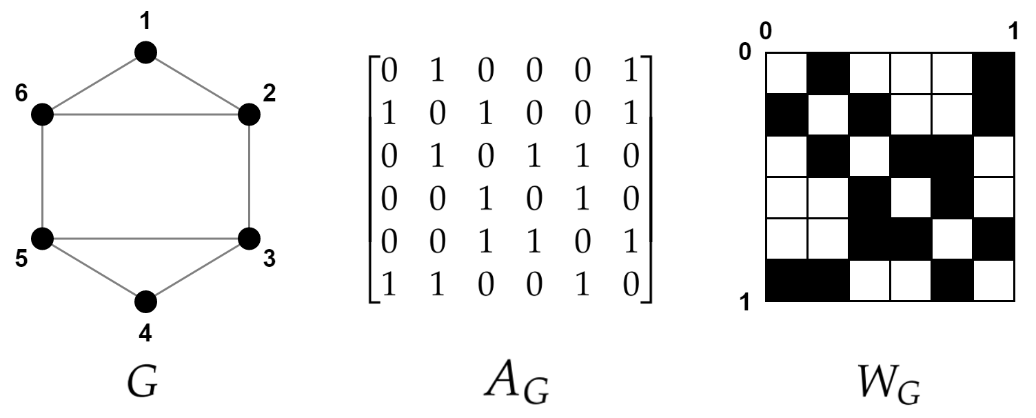
Figure 1: Graph $G$, adjacency matrix $A$ and step graphon $W_{G}$.

II-B Norms

In the study of kernels, various norms are relevant to consider [29, 31, 4]. For $1\leq p<\infty$, we define the $L^{p}$ norm of a kernel as

$$\|W\|_{L^{p}}:=\left(\int_{[0,1]^{2}}|W(x,y)|^{p}dx\;dy\right)^{1/p}$$

and its cut norm by

$$\|W\|_{\square}:=\sup_{S,T\subseteq[0,1]}\left|\int_{S\times T}W(x,y)\,dx\;dy\right|.$$

For $W\in\mathcal{W}_{1}$, we have the following inequalities between $L^{p}$ norms and the cut norm:

$$\|W\|_{\square}\leq\|W\|_{L^{1}}\leq\|W\|_{L^{2}}\leq\|W\|_{L^{1}}^{1/2}\leq 1.$$

By considering the operator $T_{W}$ associated to a kernel $W\in\mathcal{W}$, we can define the operator norm:

$${\left|\kern-1.07639pt\left|\kern-1.07639pt\left|T_{W}\right|\kern-1.07639pt\right|\kern-1.07639pt\right|}:=\sup_{\begin{subarray}{c}f\in L^{2}[0,1]\\ \|f\|_{L^{2}}=1\end{subarray}}\|T_{W}f\|_{L^{2}}.$$

For graphons, the operator norm is equal to the largest eigenvalue of the operator: ${\left|\kern-1.07639pt\left|\kern-1.07639pt\left|T_{W}\right|\kern-1.07639pt\right|\kern-1.07639pt\right|}=\lambda_{1}(T_{W})$. For the elements of $\mathcal{W}_{1}$, the cut and operator norms are related by:

$$\|W\|_{\square}\leq{\left|\kern-1.07639pt\left|\kern-1.07639pt\left|T_{W}\right|\kern-1.07639pt\right|\kern-1.07639pt\right|}\leq\sqrt{8}\|W\|_{\square}^{1/2}.$$

Finally, we can define the Hilbert-Schmidt norm of the operator as:

$$\|T_{W}\|_{\mathrm{HS}}^{2}:=\sum_{i}|\lambda_{i}(T_{W})|^{2}.$$

For all $W\in\mathcal{W}$, $\|T_{W}\|_{\mathrm{HS}}$ is finite (i.e., kernel operators are Hilbert-Schmidt operators), and moreover $\|T_{W}\|_{\mathrm{HS}}=\|W\|_{L^{2}}.$

II-C Sampling and Approximation

A graphon $W$ can be used to generate random graphs using a sampling method [29].

Definition 1 (Sampled Graph [4])

Given a graphon $W$ and a size $N\in\mathbb{N}$, we say that the graph $G$ is sampled from $W$ if it is obtained through:

1. Fixing deterministic latent variables $\{u_{i}=\frac{i}{N}\}_{i=1}^{N}$.

2. Taking $N$ vertices $\{1,\ldots,N\}$ and randomly adding undirected edges between vertices $i$ and $j$ independently with probability $W(u_{i},u_{j})$ for all $i>j$.

Definition 2 (Piecewise Lipschitz graphon [4])

Graphon $W$ is said to be piecewise Lipschitz if there exists a constant $L$ and a sequence of non-overlapping intervals $I_{k}=[\alpha_{k-1},\alpha_{k})$ defined by $0=\alpha_{0}<\cdots<\alpha_{K+1}=1$, for a finite non-negative integer $K$, such that for any $k,l$, any set $I_{kl}=I_{k}\times I_{l}$ and pairs $(x_{1},y_{1})\textrm{ and }(x_{2},y_{2})\in I_{kl}$ we have that:

$$|W(x_{1},y_{1})-W(x_{2},y_{2})|\leq L(|x_{1}-x_{2}|+|y_{1}-y_{2}|).$$

Definition 3 (Large enough $N$ [4])

Given a piecewise Lipschitz graphon $W$ (as per Definition 2) and $\nu<e^{-1}$, $N$ is large enough if $N$ satisfies the following conditions:

$$\dfrac{2}{N}<\min_{k\in\{1,\ldots,K+1\}}(\alpha_{k}-\alpha_{k-1}),$$ (1a)

$$\dfrac{1}{N}\log\left(\dfrac{2N}{\nu}\right)+\dfrac{1}{N}(2K+3L)<\max_{x}d_{W}(x),$$ (1b)

$$Ne^{-N/5}<\nu.$$ (1c)

Lemma 1 (Theorem 1 [4])

Let $W$ be a piecewise Lipschitz graphon (as per Definition 2) and $G$ a graph with $N$ nodes sampled from $W$. Then for $N$ large enough with probability at least $1-\nu$:

$${\left|\kern-1.07639pt\left|\kern-1.07639pt\left|T_{W_{G}}-T_{W}\right|\kern-1.07639pt\right|\kern-1.07639pt\right|}\leq\sqrt{\dfrac{4\log(2N/\nu)}{N}}+\dfrac{2\sqrt{L^{2}-K^{2}+KN}}{N}=:\phi(N).$$

By considering a constant value of $\nu$, the difference between the graphons in the operator norm is bounded by: ${\left|\kern-1.07639pt\left|\kern-1.07639pt\left|T_{W_{G}}-T_{W}\right|\kern-1.07639pt\right|\kern-1.07639pt\right|}=O\left((\log N/N)^{1/2}\right)$.

Lemma 2

Let $W$ be a piecewise Lipschitz graphon and $G$ a graph with $N$ nodes sampled from $W$. Then for $N$ large enough, with probability at least $1-\nu$:

$$\|W-W_{G}\|_{L^{2}}\leq\sqrt[4]{2N}\sqrt{\phi(N)}.$$

Proof:

First, we have

$$\|W-W_{G}\|_{\square}\leq{\left|\kern-1.07639pt\left|\kern-1.07639pt\left|T_{W}-T_{W_{G}}\right|\kern-1.07639pt\right|\kern-1.07639pt\right|}\leq\phi(N).$$

It is easy to see that $W_{G}$ is a step graphon that takes values in $\{0,1\}$ and we can apply the inequality derived in [31, Remark 10.8], so that:

$$\|W-W_{G}\|_{L^{1}}\leq\sqrt{2N}\|W-W_{G}\|_{\square}\leq\sqrt{2N}\phi(N).$$

Applying the relation $\|W-W_{G}\|_{L^{2}}\leq\|W-W_{G}\|_{L^{1}}^{1/2}$ yields the desired result. ∎

III SIS Epidemics

We consider a deterministic SIS model over a network modeled by a connected graph $G$ with homogeneous recovery and infection rates. The dynamics of each agent can be modeled by [17]:

$$\dot{x}_{i}(t)=-\delta x_{i}(t)+\sum_{j=1}^{N}a_{ij}\beta x_{j}(t)(1-x_{i}(t)),$$

where $x_{i}(t)\in[0,1]$ is the fraction of the $i$th subpopulation that is infected at time $t$, $\delta$ is the recovery rate and $\beta$ is the infection rate. The model of all the network can be expressed in vector form as:

$$\dot{x}(t)=(\beta A-\delta I)x(t)-\beta X(t)Ax(t),$$ (2)

where $x(t)=[x_{1}(t),x_{2}(t),\ldots,x_{N}(t)]^{T}$ is the state vector of the system, $I$ is the identity matrix, $X(t)=\mathrm{diag}[x_{1}(t),x_{2}(t),\dots,x_{N}(t)]$ is a diagonal matrix and $A$ is the adjacency matrix of the network.

III-A Stability of SIS epidemics

For any initial condition, the equilibrium $x=0$ (disease-free state) is globally asymptotically stable if the following condition is satisfied [17, Theorem 6]:

$$\lambda_{1}(A)\dfrac{\beta}{\delta}<1.$$ (3)

In the perspective approximating graphs with graphons, it is convenient to consider sequences of graphs parametrized by their size $N$. Therefore, it is reasonable to assume that parameters $\delta$ or $\beta$ be also dependent on $N$: upon need, we shall emphasize this dependence by writing $\delta_{N}$ and $\beta_{N}$.

As a first example of application of graphons, we determine a condition to reach the disease-free state for a graph sampled from $W$, based on the characteristics of the graphon.

Proposition 1 (Stability of epidemics)

Let $W$ be a piecewise Lipschitz graphon and $G$ a graph with $N$ nodes sampled from $W$, representing the network for the SIS epidemic modeled in (2). Then for $N$ large enough, the epidemic will reach the disease-free state with probability at least $1-\nu$ if:

$$\delta_{N}>N\beta_{N}({\left|\kern-1.07639pt\left|\kern-1.07639pt\left|T_{W}\right|\kern-1.07639pt\right|\kern-1.07639pt\right|}+\phi(N)).$$ (4)

Proof:

Condition (3) is equivalent to $\delta>\beta\lambda_{1}(A).$ By Lemma 1, with $N$ large enough and probability at least $1-\nu$:

$$\left|\lambda_{1}\left(T_{W_{G}}\right)-\lambda_{1}(T_{W})\right|\leq\phi(N),$$

$$\lambda_{1}\left(T_{W_{G}}\right)\leq\lambda_{1}(T_{W})+\phi(N).$$

Since $\lambda_{1}(A)=N\lambda_{1}\left(T_{W_{G}}\right)$, the above inequality yields (4). ∎

III-B An Index for the Sensitivity to Noise

When the focus is stability of the disease-free state, it is natural to study the linearization of (2) near the origin [32]:

$$\dot{x}(t)=(\beta A-\delta I)x(t)=\mathcal{A}x(t).$$ (5)

This linearization is exponentially stable [18] under condition (3). We now turn our attention to the robustness of this stability property and more precisely to quantifying how the epidemics react to noise in the neighborhood of the equilibrium. Indeed, noise can represent migrations or other phenomena that are not included in the original model [20]. To this purpose, we include additive noise in (5) and define

$$\dot{x}(t)=\mathcal{A}x(t)+n(t),$$ (6)

where $n(t)\in\mathbb{R}^{N}$ is a stochastic noise process. A measure of this sensitivity can be defined as the asymptotic mean-square error:

$$J^{\mathrm{noise}}_{G}:=\lim_{t\to\infty}\dfrac{1}{N}\mathbb{E}\left[\|x(t)\|_{2}^{2}\right].$$ (7)

Under suitable assumptions on the noise vector, this noise index is determined by the eigenvalues of the network.

Proposition 2

Consider the system given in (6) satisfying condition (3) and a noise vector with zero mean and autocorrelation function $\mathbb{E}[n(t)n(t-\xi)^{T}]=\sigma^{2}\deltaup(\xi)I$. Then, the noise index (7) can be expressed as:

$$J^{\mathrm{noise}}_{G}=\dfrac{\sigma^{2}}{2N}\sum_{i=1}^{N}\dfrac{1}{\delta-\beta\lambda_{i}(A)}.$$ (8)

Proof:

Considering that the solution of system (6) is $x(t)=e^{\mathcal{A}t}x(0)+\int_{0}^{t}e^{\mathcal{A}(t-\tau)}n(\tau)d\tau,$ we calculate the expected value of $\|x(t)\|_{2}^{2}$:

$$\mathbb{E}\left[\|x(t)\|_{2}^{2}\right]= \mathbb{E}\left[\left\|e^{\mathcal{A}t}x(0)+\int_{0}^{t}e^{\mathcal{A}(t-\tau)}n(\tau)d\tau\right\|_{2}^{2}\right]$$

$$= \mathbb{E}\left[\left\|e^{\mathcal{A}t}x(0)\right\|_{2}^{2}\right]$$ (9)

$$+2\,\mathbb{E}\left[\left(e^{\mathcal{A}t}x(0)\right)^{T}\int_{0}^{t}e^{\mathcal{A}(t-\tau)}n(\tau)d\tau\right]$$

$$+\mathbb{E}\left[\left(\int_{0}^{t}e^{\mathcal{A}(t-\tau)}n(\tau)d\tau\!\right)^{\!T}\int_{0}^{t}e^{\mathcal{A}(t-\tau)}n(\tau)d\tau\right].$$

We begin by studying the third term (hereby denoted by $U$):

$$U =\int_{0}^{t}\int_{0}^{t}\mathbb{E}\left[\left(e^{\mathcal{A}(t-\tau_{1})}n(\tau_{1})\right)^{T}\left(e^{\mathcal{A}(t-\tau_{2})}n(\tau_{2})\right)\right]d\tau_{1}d\tau_{2}.$$

Since for a real scalar $a$, we have $a=\mathrm{tr}(a)$, we can apply the trace to the integrand and its cyclic property, obtaining:

$$U =\int_{0}^{t}\int_{0}^{t}\mathbb{E}\left[\mathrm{tr}\left(e^{\mathcal{A}(t-\tau_{1})}e^{\mathcal{A}(t-\tau_{2})}n(\tau_{2})n(\tau_{1})^{T}\right)\right]d\tau_{1}d\tau_{2}$$

$$=\int_{0}^{t}\int_{0}^{t}\mathrm{tr}\left(e^{\mathcal{A}(t-\tau_{1})}e^{\mathcal{A}(t-\tau_{2})}\mathbb{E}\left[n(\tau_{2})n(\tau_{1})^{T}\right]\right)d\tau_{1}d\tau_{2}.$$

Due to the characteristics of the autocorrelation function of the noise, we have $\mathbb{E}\left[n(\tau_{2})n(\tau_{1})^{T}\right]=\sigma^{2}{\deltaup}(\tau_{2}-\tau_{1})I$. Thus:

$$U =\int_{0}^{t}\int_{0}^{t}\mathrm{tr}\left(e^{\mathcal{A}(t-\tau_{1})}e^{\mathcal{A}(t-\tau_{2})}\sigma^{2}{\deltaup}(\tau_{2}-\tau_{1})I\right)d\tau_{1}d\tau_{2}$$

$$=\sigma^{2}\mathrm{tr}\left(\int_{0}^{t}\left(\int_{0}^{t}{\deltaup}(\tau_{2}-\tau_{1})e^{\mathcal{A}(t-\tau_{1})}d\tau_{1}\right)e^{\mathcal{A}(t-\tau_{2})}d\tau_{2}\right).$$

Using linearity of the trace and Dirac’s delta property that $\int_{I_{a}}\deltaup(\tau-a)\varphi(\tau)d\tau=\varphi(a)$ for any interval $I_{a}$ that has $a$ in its interior and any test function $\varphi$, we get:

$$U=\sigma^{2}\int_{0}^{t}\mathrm{tr}\left(e^{2\mathcal{A}(t-\tau_{2})}\right)d\tau_{2}.$$

Being matrix $\mathcal{A}$ symmetric, it can be written $\mathcal{A}=Q\Lambda Q^{T}$ where $Q$ is an orthogonal matrix and $\Lambda$ is a diagonal matrix with the eigenvalues of $\mathcal{A}$. Since $e^{\mathcal{A}}=Qe^{\Lambda}Q^{T}$, we have:

$$U =\sigma^{2}\int_{0}^{t}\mathrm{tr}\left(Qe^{2\Lambda(t-\tau_{2})}Q^{T}\right)d\tau_{2}$$

$$=\sigma^{2}\int_{0}^{t}\mathrm{tr}\left(e^{2\Lambda(t-\tau_{2})}\right)d\tau_{2}$$

$$=\sigma^{2}\int_{0}^{t}\sum_{i=1}^{N}e^{2(t-\tau_{2})\lambda_{i}(\mathcal{A})}d\tau_{2}$$

$$=\sigma^{2}\sum_{i=1}^{N}e^{2t\lambda_{i}(\mathcal{A})}\int_{0}^{t}e^{-2\tau_{2}\lambda_{i}(\mathcal{A})}d\tau_{2}$$

$$=\sigma^{2}\sum_{i=1}^{N}\dfrac{1}{2\lambda_{i}(\mathcal{A})}\left[e^{2t\lambda_{i}(\mathcal{A})}-1\right].$$

We observe that the first term in (9) becomes zero when $t\rightarrow\infty$ because of condition (3), while the second term is zero because the expected value of the noise is zero. Then,

$$J^{\mathrm{noise}}_{G}=\dfrac{1}{N}\lim_{t\to\infty}\left(\sigma^{2}\sum_{i=1}^{N}\dfrac{1}{2\lambda_{i}(\mathcal{A})}\left[e^{2t\lambda_{i}(\mathcal{A})}-1\right]\right).$$

The conclusion follows because condition (3) implies that all eigenvalues of $\mathcal{A}$ are negative. ∎

Our objective is to estimate this noise index for a graph sampled from a graphon, by using the spectrum of the graphon operator. Assuming that the graphon $W$ has finite rank $M$, for all $N\geq M$ we define

$$J^{\mathrm{noise}}_{W,N}:=\dfrac{\sigma^{2}}{2N}\sum_{i=1}^{N}\dfrac{1}{\delta_{N}-\beta_{N}N\lambda_{i}(T_{W})},$$

where $\lambda_{i}(T_{W})$ are the nonzero eigenvalues of $T_{W}$ for $i=1,\ldots,M$ and $\lambda_{i}(T_{W})=0$ for $i=M+1,\ldots,N$. We will use $J^{\mathrm{noise}}_{W,N}$ as an approximation of $J^{\mathrm{noise}}_{G}$ when $G$ is a large graph sampled from $W$; Theorem 1 will ensure that the approximation error is small with high probability. Since this result involves epidemics on graphs of increasing size $N$, we have to specify the dependence on $N$ of the parameters $\delta_{N}$ and $\beta_{N}$. Clearly, we need to satisfy the stability condition (3) for all $N$: actually, we will need the stronger property that $\lambda_{1}(A_{N})\beta_{N}/\delta_{N}$ remains bounded away from $1$ also in the limit for $N\to\infty$. Since almost surely $\lambda_{1}(A_{N})$ grows linearly with $N$ (except for the trivial graphon $W=0$), in order to ensure a uniform bound on $\lambda_{1}(A_{N})\beta_{N}/\delta_{N}$, we will assume that the infection strength $\beta_{N}/\delta_{N}$ satisfies

$$\frac{\beta_{N}}{\delta_{N}}=\frac{1}{N}\frac{\bar{\beta}}{\bar{\delta}}$$ (10)

for some positive constants $\bar{\beta}$ and $\bar{\delta}$.

Theorem 1 (Graphon approximation)

Let $W$ be a piecewise Lipschitz graphon with finite rank $M$ and $G$ a graph with $N$ nodes sampled from $W$ with $N\geq M$. If $\delta_{N}=\bar{\delta}$ and $\beta_{N}=N^{-1}\bar{\beta}$ satisfy condition (4), then for $N$ large enough, with probability at least $1-\nu$:

$$\Delta^{\mathrm{noise}} :=\left|J^{\mathrm{noise}}_{G}-J^{\mathrm{noise}}_{W,N}\right|$$

$$\leq\dfrac{1}{N^{{3}/4}}\dfrac{\sigma^{2}\bar{\beta}\sqrt{\sqrt{N\log(2N/\nu)}+\sqrt{L^{2}-K^{2}+KN}}}{\sqrt[4]{2}(\bar{\delta}-\bar{\beta}{\left|\kern-1.07639pt\left|\kern-1.07639pt\left|T_{W}\right|\kern-1.07639pt\right|\kern-1.07639pt\right|}-\bar{\beta}\phi(N))(\bar{\delta}-\bar{\beta}{\left|\kern-1.07639pt\left|\kern-1.07639pt\left|T_{W}\right|\kern-1.07639pt\right|\kern-1.07639pt\right|})}.$$

Proof:

Throughout this proof, we will assume that $\lambda_{i}(T_{W})$ (i.e., the $M$ non-zero eigenvalues of $T_{W}$ and $N-M$ zeros) are sorted in non-increasing order: this choice does not change the sum that defines $J^{\mathrm{noise}}_{W,N}$ and is consistent with the non-increasing ordering of $\lambda_{i}(A)$. This consistency will be useful in order to apply Wielandt-Hoffman Theorem. Since $\lambda_{i}(A)=N\lambda_{i}\left(T_{W_{G}}\right)$, $\delta_{N}=\bar{\delta}$ and $\beta_{N}=N^{-1}\bar{\beta}$, we have:

$$\Delta^{\mathrm{noise}} =\left|\dfrac{\sigma^{2}}{2N}\sum_{i=1}^{N}\dfrac{1}{\delta_{N}-\beta_{N}\lambda_{i}(A)}-\dfrac{\sigma^{2}}{2N}\sum_{i=1}^{N}\dfrac{1}{\delta_{N}-N\beta_{N}\lambda_{i}(T_{W})}\right|$$

$$=\dfrac{\sigma^{2}}{2N}\left|\sum_{i=1}^{N}\dfrac{1}{\bar{\delta}-\bar{\beta}\lambda_{i}\left(T_{W_{G}}\right)}-\sum_{i=1}^{N}\dfrac{1}{\bar{\delta}-\bar{\beta}\lambda_{i}(T_{W})}\right|$$

$$=\dfrac{\sigma^{2}\bar{\beta}}{2N}\left|\sum_{i=1}^{N}\dfrac{\lambda_{i}(T_{W})-\lambda_{i}\left(T_{W_{G}}\right)}{\left(\bar{\delta}-\bar{\beta}\lambda_{i}\left(T_{W_{G}}\right)\right)(\bar{\delta}-\bar{\beta}\lambda_{i}(T_{W}))}\right|$$

$$\leq\dfrac{\sigma^{2}\bar{\beta}}{2N}\sum_{i=1}^{N}\dfrac{\left|\lambda_{i}(T_{W})-\lambda_{i}\left(T_{W_{G}}\right)\right|}{\left(\bar{\delta}-\bar{\beta}\lambda_{i}\left(T_{W_{G}}\right)\right)(\bar{\delta}-\bar{\beta}\lambda_{i}(T_{W}))}$$

$$\leq\dfrac{\sigma^{2}\bar{\beta}\sum_{i=1}^{N}\left|\lambda_{i}(T_{W})-\lambda_{i}\left(T_{W_{G}}\right)\right|}{2N\left(\bar{\delta}-\bar{\beta}{\left|\kern-1.07639pt\left|\kern-1.07639pt\left|T_{W_{G}}\right|\kern-1.07639pt\right|\kern-1.07639pt\right|}\right)(\bar{\delta}-\bar{\beta}{\left|\kern-1.07639pt\left|\kern-1.07639pt\left|T_{W}\right|\kern-1.07639pt\right|\kern-1.07639pt\right|})}.$$

We define the vector $\lambda_{T_{W}-T_{W_{G}}}$ as:

$$\lambda_{T_{W}-T_{W_{G}}}=\left[\lambda_{1}(T_{W})-\lambda_{1}\left(T_{W_{G}}\right),\ldots,\lambda_{N}(T_{W})-\lambda_{N}\left(T_{W_{G}}\right)\right]^{T},$$

so that the sum in the numerator is

$$\sum_{i=1}^{N}\left|\lambda_{i}(T_{W})-\lambda_{i}\left(T_{W_{G}}\right)\right|=\left\|\lambda_{T_{W}-T_{W_{G}}}\right\|_{1}.$$

Then, the relation $\|\cdot\|_{1}\leq\sqrt{N}\|\cdot\|_{2}$ implies

$$\Delta^{\mathrm{noise}}\leq\dfrac{\sigma^{2}\bar{\beta}\left(\sum_{i=1}^{N}\left|\lambda_{i}(T_{W})-\lambda_{i}\left(T_{W_{G}}\right)\right|^{2}\right)^{1/2}}{2N^{1/2}\left(\bar{\delta}-\bar{\beta}{\left|\kern-1.07639pt\left|\kern-1.07639pt\left|T_{W_{G}}\right|\kern-1.07639pt\right|\kern-1.07639pt\right|}\right)(\bar{\delta}-\bar{\beta}{\left|\kern-1.07639pt\left|\kern-1.07639pt\left|T_{W}\right|\kern-1.07639pt\right|\kern-1.07639pt\right|})}.$$

We can apply Wielandt-Hoffman Theorem in infinite dimensional spaces [33, Theorem 2] and, since $N\geq M$, get:

$$\Delta^{\mathrm{noise}}\leq\dfrac{\sigma^{2}\bar{\beta}\left\|T_{W}-T_{W_{G}}\right\|_{\mathrm{HS}}}{2N^{1/2}\left(\bar{\delta}-\bar{\beta}{\left|\kern-1.07639pt\left|\kern-1.07639pt\left|T_{W_{G}}\right|\kern-1.07639pt\right|\kern-1.07639pt\right|}\right)(\bar{\delta}-\bar{\beta}{\left|\kern-1.07639pt\left|\kern-1.07639pt\left|T_{W}\right|\kern-1.07639pt\right|\kern-1.07639pt\right|})}.$$

Since $\left\|T_{W}-T_{W_{G}}\right\|_{\mathrm{HS}}=\|W-W_{G}\|_{L^{2}}$, Lemma 2 implies that

$$\Delta^{\mathrm{noise}}\leq\dfrac{\sigma^{2}\bar{\beta}\sqrt[4]{2N}\sqrt{\phi(N)}}{2N^{1/2}\left(\bar{\delta}-\bar{\beta}{\left|\kern-1.07639pt\left|\kern-1.07639pt\left|T_{W_{G}}\right|\kern-1.07639pt\right|\kern-1.07639pt\right|}\right)(\bar{\delta}-\bar{\beta}{\left|\kern-1.07639pt\left|\kern-1.07639pt\left|T_{W}\right|\kern-1.07639pt\right|\kern-1.07639pt\right|})},$$

and the proof is completed by using the definition of $\phi(N)$ and applying Lemma 1 in the denominator. ∎

Assuming that $\delta=\bar{\delta}$ is constant and $\beta=N^{-1}\bar{\beta}$ means that, as the graph grows in size, the healing rate (which depends on each individual) remains constant, whereas the infection rate decreases. This natural scaling law is also chosen in [7]. Indeed, on dense graphs this assumption means that in larger graphs, even though there are more potential interactions, the average strength of the connections is suitably adjusted: this fact accounts for natural limitations in the rates of contact between individuals.

Remark 1 (Asymptotics for $N\to\infty$ & scaling factors)

When we let $N$ go to infinity, if $\nu$ is constant or if $\nu=N^{\alpha}$ for some constant $\alpha$, we can see that the upper bound given in Theorem 1 for the estimation error $\Delta^{\mathrm{noise}}$ goes to zero as $O\left((\log N)^{1/4}/(N^{1/2})\right)$. Hence, by choosing $\alpha>1$ and applying Borel-Cantelli Lemma, we obtain that $\Delta^{\mathrm{noise}}$ almost surely converges to zero with rate $O\left((\log N)^{1/4}/(N^{1/2})\right)$. Index $J^{\mathrm{noise}}_{G}$ is bounded and bounded away from zero under the assumptions of Theorem 1. Hence, the same asymptotic behaviour holds for the relative error $\Delta^{\mathrm{noise}}/J^{\mathrm{noise}}_{G}$. This asymptotic behaviour of the relative error does not depend on the assumption $\beta_{N}=N^{-1}\bar{\beta}$ and remains true for any choice of $\delta_{N}$ and $\beta_{N}$ that satisfies (4) and (10). Indeed, any other choice of $\delta_{N}$ and $\beta_{N}$ satisfying (10) would modify both $J^{\mathrm{noise}}_{G}$ and $J^{\mathrm{noise}}_{W,N}$ by the same multiplicative factor, so that the relative error would remain the same.

IV Numerical and Simulation Results

We consider the stochastic block model graphon $W_{\mathrm{SB}}$ with pixel diagram in Fig. 2, where the values of the blocks are:

$$W_{\mathrm{SB}}=\begin{bmatrix}0.9&0.7&0.6&0.5&0.2\\ 0.7&0.4&0.1&0.3&0.1\\ 0.6&0.1&0.5&0.9&0.8\\ 0.5&0.3&0.9&0.5&0.5\\ 0.2&0.1&0.8&0.5&0.7\end{bmatrix}.$$

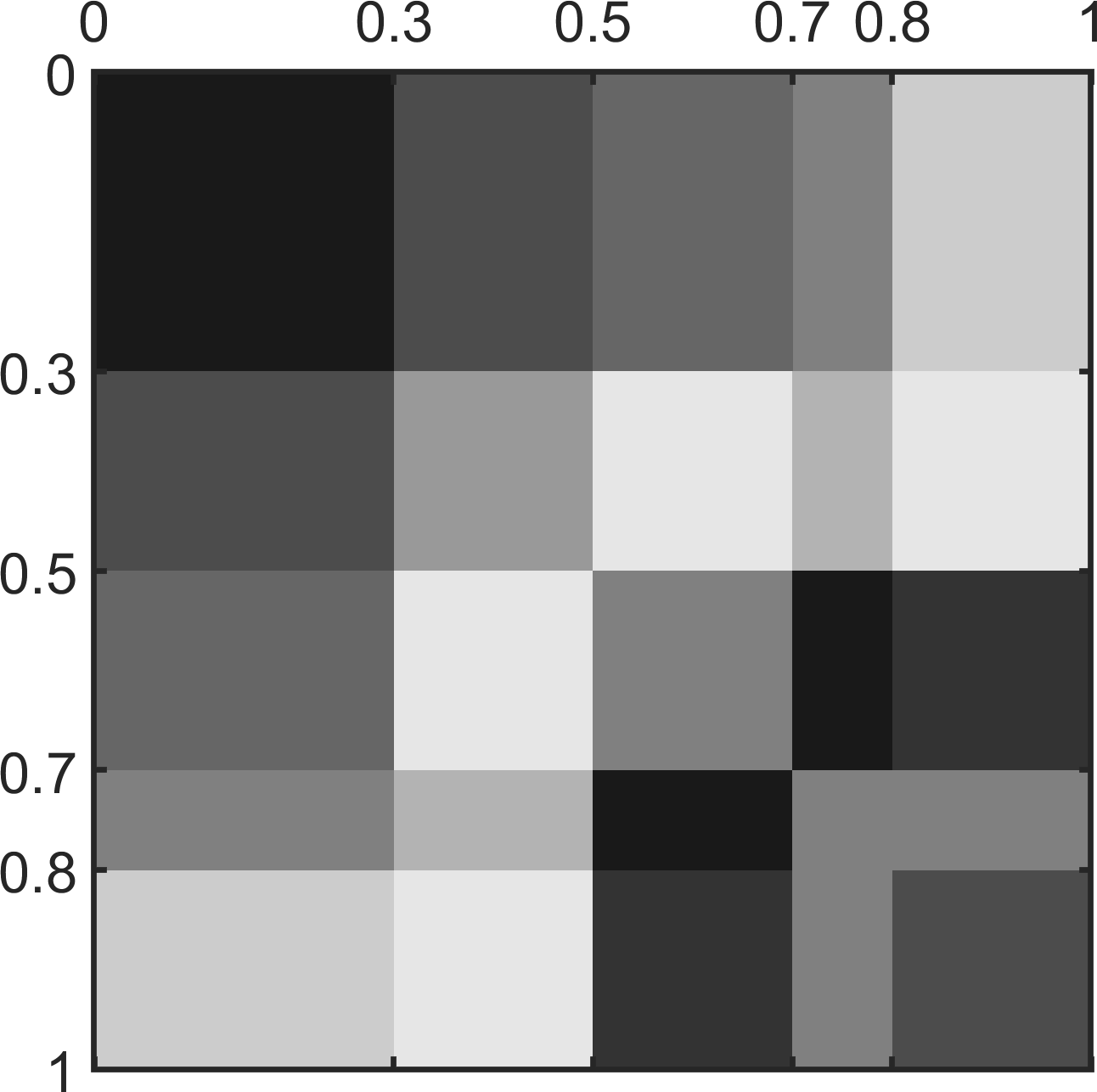
Figure 2: Pixel diagram of the stochastic block model graphon.

The nonzero eigenvalues of the graphon operator $T_{W_{\mathrm{SB}}}$ are $\lambda_{1}=0.5275$, $\lambda_{2}=0.2098$, $\lambda_{3}=0.0126$, $\lambda_{4}=-0.0128$ and $\lambda_{5}=-0.0971$. We assume $\beta_{N}=\bar{\beta}=0.1$ and $\nu=0.02$, which satisfies condition (1c) for $N\geq 40$, and we generate sampled graphs from $W_{SB}$ with $40\leq N\leq 1000$. For each network, the value of $\delta_{N}=N\bar{\delta}=N\bar{\beta}({\left|\kern-1.07639pt\left|\kern-1.07639pt\left|T_{W}\right|\kern-1.07639pt\right|\kern-1.07639pt\right|}+\phi(40))$ is selected, satisfying condition (4), and we compute the relative error $\Delta^{\mathrm{noise}}/J^{\mathrm{noise}}_{G}$, obtaining the results of Fig. 3. As per Remark 1, the relative error goes to zero as $N$ increases.

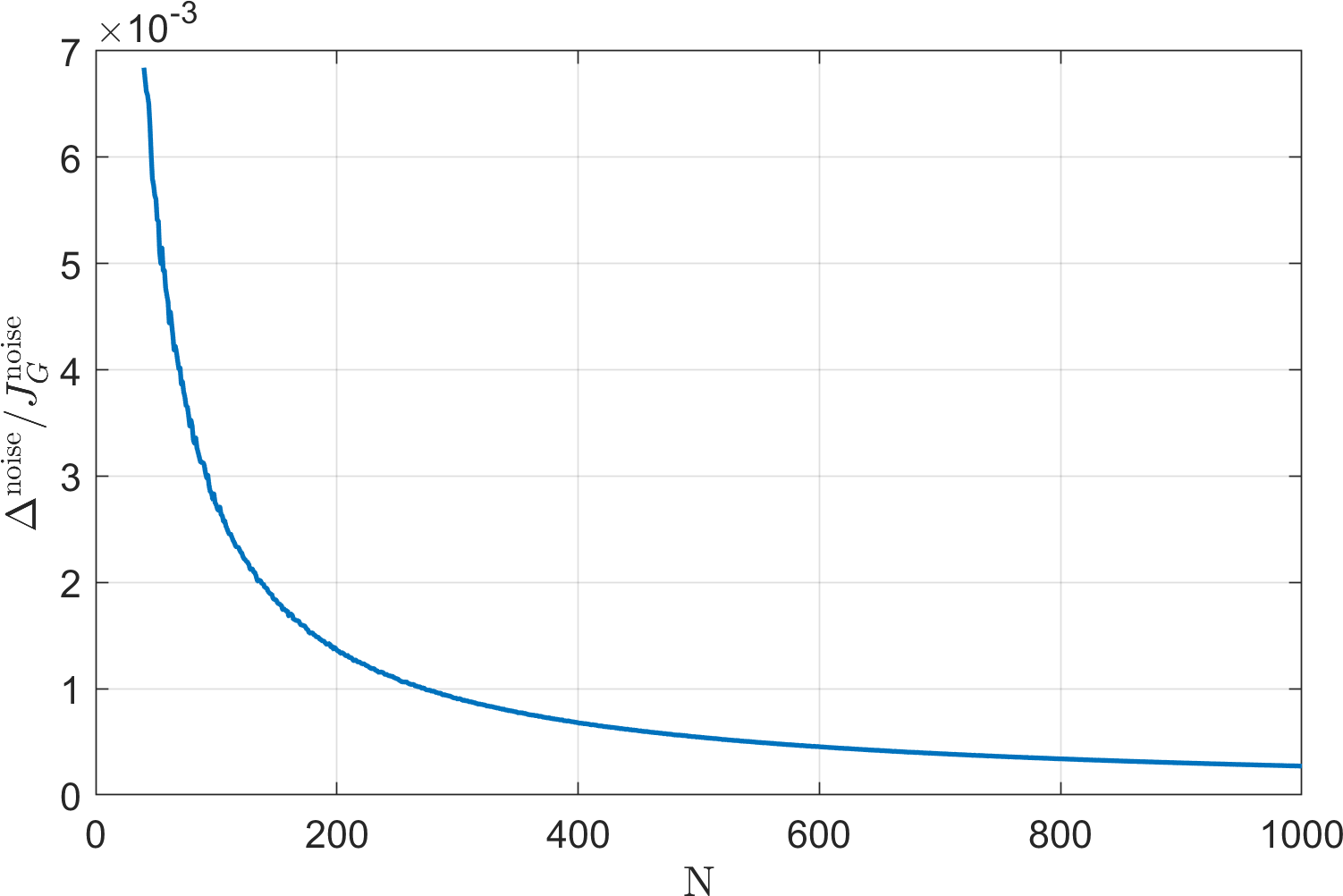
Figure 3: Relative error $\Delta^{\mathrm{noise}}/J^{\mathrm{noise}}_{G}$ as a function of $N$ for the stochastic block model in Fig. 2.

V Conclusion

This work presented an analysis of SIS epidemics on large networks, under the assumption that the network is sampled from a graphon. Relevant information about the stability of an epidemic can be inferred from the graphon, without the need to perform computations on, or even know, the full network topology. In this vein, we have derived a stability criterion in Proposition 1 and defined a noise-sensitivity index (Theorem 1) that both only depend on the graphon.

Several questions are left open by this work, including the extension of our results to networks sampled from graphons that do not have finite rank: this extension could be enabled by the spectral approximation tools developed in [7]. Moreover, we believe that graphons can help not only the analysis but also the control of epidemics: for instance, graphon centrality [4] can provide guidance for targeted interventions such as quarantine or vaccination.

References

• [1] L. Lovász and B. Szegedy, “Limits of dense graph sequences,” Journal of Combinatorial Theory, Series B, vol. 96, no. 6, pp. 933–957, 2006.
• [2] C. Borgs, J. T. Chayes, L. Lovász, V. T. Sós, and K. Vesztergombi, “Convergent sequences of dense graphs I: Subgraph frequencies, metric properties and testing,” Advances in Mathematics, vol. 219, no. 6, pp. 1801–1851, 2008.
• [3] ——, “Convergent sequences of dense graphs II. Multiway cuts and statistical physics,” Annals of Mathematics, vol. 176, no. 1, pp. 151–219, 2012.
• [4] M. Avella-Medina, F. Parise, M. Schaub, and S. Segarra, “Centrality measures for graphons: Accounting for uncertainty in networks,” IEEE Transactions on Network Science and Engineering, 2018.
• [5] Y. Zhang, E. Levina, and J. Zhu, “Estimating network edge probabilities by neighbourhood smoothing,” Biometrika, vol. 104, no. 4, pp. 771–783, 2017.
• [6] C. Kuehn and S. Throm, “Power network dynamics on graphons,” SIAM Journal on Applied Mathematics, vol. 79, no. 4, pp. 1271–1292, 2019.
• [7] S. Gao and P. E. Caines, “Spectral representations of graphons in very large network systems control,” in IEEE Conference on Decision and Control, 2019, pp. 5068–5075.
• [8] ——, “The control of arbitrary size networks of linear systems via graphon limits: An initial investigation,” in IEEE Conference on Decision and Control, 2017, pp. 1052–1057.
• [9] ——, “Optimal and approximate solutions to linear quadratic regulation of a class of graphon dynamical systems,” in IEEE Conference on Decision and Control, 2019, pp. 8359–8365.
• [10] ——, “Graphon control of large-scale networks of linear systems,” IEEE Transactions on Automatic Control, 2019.
• [11] P. E. Caines and M. Huang, “Graphon mean field games and the GMFG equations,” in IEEE Conference on Decision and Control, 2018, pp. 4129–4134.
• [12] F. Parise and A. Ozdaglar, “Graphon games,” in ACM Conference on Economics and Computation, 2019, pp. 457–458.
• [13] A. Lajmanovich and J. A. Yorke, “A deterministic model for gonorrhea in a nonhomogeneous population,” Mathematical Biosciences, vol. 28, no. 3-4, pp. 221–236, 1976.
• [14] N. T. Bailey, “Macro-modelling and prediction of epidemic spread at community level,” Mathematical Modelling, vol. 7, no. 5-8, pp. 689–717, 1986.
• [15] R. Pastor-Satorras, C. Castellano, P. Van Mieghem, and A. Vespignani, “Epidemic processes in complex networks,” Reviews of modern physics, vol. 87, no. 3, p. 925, 2015.
• [16] P. E. Paré, J. Liu, C. L. Beck, B. E. Kirwan, and T. Başar, “Analysis, estimation, and validation of discrete-time epidemic processes,” IEEE Transactions on Control Systems Technology, vol. 28, no. 1, pp. 79–93, 2020.
• [17] C. Nowzari, V. M. Preciado, and G. J. Pappas, “Analysis and control of epidemics: A survey of spreading processes on complex networks,” IEEE Control Systems Magazine, vol. 36, no. 1, pp. 26–46, 2016.
• [18] W. Mei, S. Mohagheghi, S. Zampieri, and F. Bullo, “On the dynamics of deterministic epidemic propagation over networks,” Annual Reviews in Control, vol. 44, pp. 116–128, 2017.
• [19] G. Zhu, X. Fu, and G. Chen, “Spreading dynamics and global stability of a generalized epidemic model on complex heterogeneous networks,” Applied Mathematical Modelling, vol. 36, no. 12, pp. 5808–5817, 2012.
• [20] E. Forgoston, S. Bianco, L. B. Shaw, and I. B. Schwartz, “Maximal sensitive dependence and the optimal path to epidemic extinction,” Bulletin of mathematical biology, vol. 73, no. 3, pp. 495–514, 2011.
• [21] P. E. Paré, C. L. Beck, and A. Nedić, “Epidemic processes over time-varying networks,” IEEE Transactions on Control of Network Systems, vol. 5, no. 3, pp. 1322–1334, 2017.
• [22] A. L. Krause, L. Kurowski, K. Yawar, and R. A. Van Gorder, “Stochastic epidemic metapopulation models on networks: SIS dynamics and control strategies,” Journal of theoretical biology, vol. 449, pp. 35–52, 2018.
• [23] F. Fagnani and P. Frasca, Introduction to Averaging Dynamics over Networks.   Springer, 2018.
• [24] X. Ma and N. Elia, “Mean square performance and robust yet fragile nature of torus networked average consensus,” IEEE Transactions on Control of Network Systems, vol. 2, no. 3, pp. 216–225, 2015.
• [25] E. Lovisari and S. Zampieri, “Performance metrics in the average consensus problem: a tutorial,” Annual Reviews in Control, vol. 36, no. 1, pp. 26–41, 2012.
• [26] F. Garin and L. Schenato, “A survey on distributed estimation and control applications using linear consensus algorithms,” in Networked Control Systems.   Springer, 2010, pp. 75–107.
• [27] P. W. Holland, K. B. Laskey, and S. Leinhardt, “Stochastic blockmodels: First steps,” Social networks, vol. 5, no. 2, pp. 109–137, 1983.
• [28] B. Karrer and M. E. Newman, “Stochastic blockmodels and community structure in networks,” Physical review E, vol. 83, no. 1, p. 016107, 2011.
• [29] L. Lovász, Large Networks and Graph Limits.   American Mathematical Society, 2012.
• [30] E. M. Airoldi, T. B. Costa, and S. H. Chan, “Stochastic blockmodel approximation of a graphon: Theory and consistent estimation,” in Advances in Neural Information Processing Systems, 2013, pp. 692–700.
• [31] S. Janson, Graphons, cut norm and distance, couplings and rearrangements.   NYJM Monographs, 2013, no. 3.
• [32] A. Khanafer and T. Başar, “An optimal control problem over infected networks,” in International Conference of Control, Dynamic Systems, and Robotics, 2014.
• [33] R. Bhatia and L. Elsner, “The Hoffman-Wielandt inequality in infinite dimensions,” vol. 104, no. 3, pp. 483–494, 1994.