On the Robustness of Data-Driven Controllers for Linear Systems

Abstract

This paper proposes a new framework and several results to quantify the performance of data-driven state-feedback controllers for linear systems against targeted perturbations of the training data. We focus on the case where subsets of the training data are randomly corrupted by an adversary, and derive lower and upper bounds for the stability of the closed-loop system with compromised controller as a function of the perturbation statistics, size of the training data, sensitivity of the data-driven algorithm to perturbation of the training data, and properties of the nominal closed-loop system. Our stability and convergence bounds are probabilistic in nature, and rely on a first-order approximation of the data-driven procedure that designs the state-feedback controller, which can be computed directly using the training data. We illustrate our findings via multiple numerical studies.

1 Introduction

Data-driven algorithms are becoming increasingly more popular to solve a variety of engineering problems, ranging from computer vision and speech recognition to the design of stabilizing controllers for dynamical systems (e.g., see [Tabuada et al. (2017), Recht (2018)]). While providing competitive performance under nominal operating conditions and accurate data, these data-driven methods typically offer no robustness guarantees against accidental or adversarial manipulation of the training data, as demonstrated by unfortunate incidents (Poland et al., 2018) and early studies (Persis and Tesi, 2019; Dean et al., 2019; Makdah et al., 2019, 2020). This creates concerns and poses critical limitations on the deployment of data-driven control algorithms for practical problems.

In this paper we propose a novel framework and certain bounds to characterize the robustness of data-driven state-feedback controllers against perturbation of the training data. In particular, we view a data-driven algorithm to design a stabilizing state-feedback controller as a (differentiable) map from the collected data to the space of controllers. Then, we compute a first-order approximation of such map, which inherently measures the sensitivity of the data-driven control algorithm to perturbations of its input data, and use it to derive lower and upper bounds for the stability of the closed-loop system with the controller obtained from the perturbed data. Our stability results are probabilistic in nature, and they explicitly depend upon the statistics of the perturbation, the size of the training data of the data-driven algorithm, the sensitivity of the data-driven algorithm, and the spectral properties of the nominal closed-loop dynamics. Our results can be used to provide stability guarantees for data-driven controllers, as well as to compare the effectiveness of different data-driven procedures. Finally, we illustrate our findings through a numerical example.

We will make use of the following notation. The cardinality of a set $S$ is denoted by $|S|$. The spectral radius and trace of a square matrix are denoted by $\rho(\cdot)$ and $\mathrm{tr}(\cdot)$, resp. The symbol $\|\cdot\|$ denotes the Euclidean norm. The operators vec($\cdot$) and vec${}^{-1}(\cdot)$ denote the vectorization and inverse vectorization of a matrix and a vector, respectively. The probability of an event is denoted by $\mathbb{P}(\cdot)$, and the expectation of a random variable is represented by $\mathbb{E}[\cdot]$. $\mathcal{N}(0,\Sigma)$ denotes a zero-mean Gaussian distribution with covariance $\Sigma$. The complementary cumulative distribution function (CDF) of the standard normal distribution and the error function are denoted by $\mathbb{Q}(\cdot)$ and $\text{erf}(\cdot)$.

2 Problem Setup

We consider a discrete-time linear time-invariant system given by

$$x(t+1) =Ax(t)+Bu(t),\qquad t\geq 0,$$ (1)

where $x\in\mathbb{R}^{n}$, $u\in\mathbb{R}^{m}$, $A\in{}^{n\times n}$, and $B\in{}^{n\times m}$ denote, respectively, the state, the input, the system matrix, and the input matrix. We assume that the system matrices $A$ and $B$ are unknown, and that a set of control experiments have been conducted to generate training data consisting of pairs of input sequences and samples of the system trajectories. Specifically, the training data is

$$U=\begin{bmatrix}u_{1}&\cdots&u_{N}\end{bmatrix}\in\mathbb{R}^{mT\times N},\quad\text{ and }\quad X=C\begin{bmatrix}x_{1}&\cdots&x_{N}\end{bmatrix}\in\mathbb{R}^{p\times N},$$ (2)

where $N\in\mathbb{N}$ and $T\in\mathbb{N}$ denote the number and length of the control experiments, respectively, $u_{i}$ and $x_{i}$ the input and state trajectory of the $i$-th experiment, and $C\in{}^{p\times nT}$ identifies the samples of the state trajectories measured during each experiment. For instance, if $C=[0\;\cdots\;0\;I]$, then only the state at time $T$ is measured during each experiment, as in Baggio et al. (2019). Similarly, if $C=I$, then the whole trajectory is measured as, for instance, in Persis and Tesi (2019).

We assume that a static state-feedback data-driven controller $u=Kx$ is used to stabilize the system (1), where $K=F(U,X)$ and $F:{}^{mT\times N}\times{}^{p\times N}\rightarrow{}^{m\times n}$. The map $F$ denotes an arbitrary data-driven algorithm to compute stabilizing controllers, such as the procedures described in Persis and Tesi (2019) and Valadbeigi et al. (2019). We make the following assumptions:

• The controller $K=F(U,X)$ stabilizes (1), that is, $\rho(A+BK)<1$.

• The closed-loop matrix $A_{\text{cl}}=A+BK$ is diagonalizable.

• The map $F(U,X)$ is Fréchet differentiable with respect to $X$, and admits a first-order Taylor expansion. Formally, for any $Z\in\mathbb{R}^{p\times N}$ the data-driven map satisfies

  $$\mathrm{vec}(F(U,X+Z))=\mathrm{vec}(F(U,X))+J_{X}(U,X)\mathrm{vec}(Z)+R(U,X,Z),$$ (3)

  with $\underset{\|Z\|\to 0}{\lim}\frac{\|R(U,X,Z)\|}{\|Z\|}=0$, where $J_{X}$ is the Jacobian matrix consisting of partial derivatives.

We remark that Assumption (A1) requires the data-driven algorithm to stabilize the system with nominal data. Instead, Assumption (A2) is convenient for the analysis and is not restrictive. Finally, Assumption (A3) is a working assumption of this paper and is typically used in similar studies.

The main objective of this paper is to quantify the robustness of the data-driven controller $K=F(U,X)$ to perturbations of the experimental data, which can be due, for instance, to measurement noise or targeted adversarial manipulation of the data collection sensors. To this aim, let $\widetilde{X}=X+Z$ denote the data perturbed by the zero-mean random noise $Z$. Let $\mathrm{supp}(Z)$ denote the set of compromised entries of $X$, that is, $\mathrm{supp}(Z)=\{i\;:\;z_{i}\neq 0\}$, with $z_{i}$ the $i$-th component of $\mathrm{vec}(Z)$. Then, the main objective of this paper is to characterize whether the perturbed closed-loop matrix ${\widetilde{A}}_{\textup{cl}}=A+B\widetilde{K}$ is stable as a function of the perturbation statistics, where $\widetilde{K}=F(U,\widetilde{X})$ denotes the data-driven controller computed with the perturbed data. Notice that $Z$ is a random matrix, and so are $\widetilde{X}$, $\widetilde{K}$, and ${\widetilde{A}}_{\textup{cl}}$. Thus, the stability of ${\widetilde{A}}_{\textup{cl}}$ will be studied in a probabilistic framework.

3 Robustness results for data-driven state-feedback controllers

In this section we study the stability properties of the perturbed closed-loop system ${\widetilde{A}}_{\textup{cl}}=A+B\widetilde{K}$. In particular, we provide bounds for $\mathbb{P}[\rho({\widetilde{A}}_{\textup{cl}})\geq 1]$, which is a well-defined random variable (see (Bharucha-Reid, 1973, p. 85)) and quantifies the probability that the closed loop system ${\widetilde{A}}_{\textup{cl}}$ is unstable. We start with the following instrumental result to approximate the matrix ${\widetilde{A}}_{\textup{cl}}$.

Lemma 3.1.

(First-order approximation of $\widetilde{A}_{\mathrm{cl}}$) Let ${J}^{\textup{v}}_{i}$ denote the $i$-th column of $J_{X}(U,X)$ in (3), and let $J_{i}=\mathrm{vec}^{-1}({J}^{\textup{v}}_{i})$. Then, for any $\tau>0$, the perturbed closed-loop matrix satisfies

$$\lim_{\mathbb{E}[\|\mathrm{vec}(Z)\|]\rightarrow 0}\mathbb{P}\left[\left\|\widetilde{A}_{\mathrm{cl}}-A_{\mathrm{cl}}-\textstyle\sum_{\mathrm{supp}(Z)}z_{i}BJ_{i}\right\|\geq\tau\sqrt{\mathbb{E}[\|\mathrm{vec}(Z)\|]}\right]\to 0.$$

Proof 3.2.

From (3) we have $\widetilde{K}=K+\textstyle\sum_{i=1}^{d}z_{i}\mathrm{vec}^{-1}({J}^{\textup{v}}_{i})+\mathrm{vec}^{-1}(R)$. Since $\ \widetilde{A}_{\mathrm{cl}}=A_{\mathrm{cl}}+B\widetilde{K}$, it now follows that $B\mathrm{vec}^{-1}(R)=\widetilde{A}_{\mathrm{cl}}-A_{\mathrm{cl}}+\textstyle\sum_{i=1}^{d}z_{i}BJ_{i}$. By invoking (Kollo and von Rosen, 2005, Theorem. 3.1.1), we note that $\mathbb{P}\left[\|B\mathrm{vec}^{-1}(R)\|\geq\tau\sqrt{\mathbb{E}[\|\mathrm{vec}(Z)\|]}\right]\to 0$ as $\mathbb{E}[\|\mathrm{vec}(Z)\|]\to 0$.

Lemma 3.1 states that, if the expected norm of the perturbation $Z$ is sufficiently small, then $\widetilde{A}_{\mathrm{cl}}$ can be well approximated as $A_{\mathrm{cl}}+\textstyle\sum_{\mathrm{supp}(Z)}z_{i}BJ_{i}$. Thus, in what follows we let

$$\widetilde{A}_{\mathrm{cl}}=A_{\mathrm{cl}}+\textstyle\sum_{\mathrm{supp}(Z)}z_{i}BJ_{i}.$$ (4)

The right hand term in (4) captures the effect of each perturbation entry of $Z$ on the nominal system $A_{\mathrm{cl}}$ in an additive form. In particular, the matrix $J_{i}$, consisting of partial derivatives of the data-driven control map $F(U,X)$ with respect to $X$, captures the sensitivity of the data-driven controller to variations of the $i$-th component of $\mathrm{vec}(X)$. Also, the specific form of the perturbation matrix allows us to capture the effect of a particular subset of the data on the controller’s performance, since $z_{i}=0$ if $i\not\in\mathrm{supp}(Z)$. Using (4), we now present bounds on the stability of the closed-loop system for the case of normally distributed perturbations. Our bounds make use of recent concentration inequality results for the sum of random matrices (Tropp, 2015; Boucheron et al., 2013).

Theorem 3.3.

(Probabilistic bounds on the stability of $\widetilde{A}_{\mathrm{cl}}$) Let $z_{i}\sim\mathcal{N}(0,\sigma_{i}^{2})$, with $i\in\mathrm{supp}(Z)$. Let $J_{i}$ be as in Lemma 3.1, and define the following parameters:

$$\overline{v}=\mathrm{max}\left\{\left\|\sum\limits_{\mathrm{supp}(Z)}\sigma_{i}^{2}BJ_{i}\left(BJ_{i}\right)^{\mathsf{T}}\right\|,\left\|\sum\limits_{\mathrm{supp}(Z)}\sigma^{2}_{i}\left(BJ_{i}\right)^{\mathsf{T}}BJ_{i}\right\|\right\},\text{ and }\underline{v}=\textstyle\sum\limits_{\mathrm{supp}(Z)}\sigma^{2}_{i}\left[\mathrm{tr}(BJ_{i})\right]^{2}.$$

Let $\kappa=\|A_{\mathrm{cl}}\|\|A_{\mathrm{cl}}^{-1}\|$ be the condition number of $A_{\mathrm{cl}}$, and let $\mu=\mathrm{tr}(A_{\mathrm{cl}})$. Then,

$$\mathbb{Q}\left(\frac{n+\mu}{\sqrt{\underline{v}}}\right)+\mathbb{Q}\left(\frac{n-\mu}{\sqrt{\underline{v}}}\right)\leq\mathbb{P}\left[\rho(\widetilde{A}_{\mathrm{cl}})\geq 1\right]\leq 2n\exp\left(\frac{-\left(1-\rho(A_{\mathrm{cl}})\right)^{2}}{(2\overline{v})\kappa^{2}}\right).$$ (5)

Proof 3.4.

Let $\Delta=\sum_{\mathrm{supp}(Z)}z_{i}BJ_{i}$. From (4) we have the following estimate:

$$n^{-1}|\mathrm{tr}(\widetilde{A}_{\mathrm{cl}})|\leq\rho(\widetilde{A}_{\mathrm{cl}})\leq\rho(A_{\mathrm{cl}})+\kappa\|\Delta\|.$$ (6)

The second inequality in (6) follows from the Bauer-Fike Theorem (Stewart and Ji-guang Sun, 1990, Chapter 4). Instead, the first inequality is trivially obtained using the triangle inequality.

(Upper bound) Let $t=(1-\rho(A_{\text{cl}}))/\kappa$ and $\widetilde{\Delta}=\sum_{\mathrm{supp}(Z)}\tilde{z}_{i}(\sigma_{i}BJ_{i})$, where $\tilde{z}_{i}$ are independent and identically distributed random variables with zero mean and unit variance, which are also independent of the perturbation variables $z_{i}$. Notice the following chain of inequalities:

$$\mathbb{P}[\rho(\widetilde{A}_{\text{cl}})\geq 1]\leq\mathbb{P}\left[\rho(A_{\mathrm{cl}})+\kappa\|\Delta\|\geq 1\right]=\mathbb{P}\left[\|\Delta\|\geq t\right]=\mathbb{P}\left[\|\widetilde{\Delta}\|\geq t\right]\leq(2n)\exp({-t^{2}}/{2\overline{v}}).$$

The first inequality follows by invoking monotonicity of probabilities on the set inclusion $\{\rho(\widetilde{A}_{\text{cl}})\geq 1\}\subseteq\left\{\rho(A_{\mathrm{cl}})+\kappa\|\Delta\|\geq 1\right\}$. The second equality follows from the fact that the random matrices $\Delta$ and $\widetilde{\Delta}$ are equal in distribution. The last inequality follows from (Tropp, 2015, Theorem. 4.1.1).

(Lower bound) From (6), consider the set inclusion $\{|\mathrm{tr}(\widetilde{A}_{\mathrm{cl}})|\geq n\}\subseteq\{\rho(\widetilde{A}_{\text{cl}})\geq 1\}$, which implies $\mathbb{P}[|\mathrm{tr}(\widetilde{A}_{\mathrm{cl}})|\geq n]\leq\mathbb{P}[\rho(\widetilde{A}_{\mathrm{cl}})\geq 1]$. Further, from (4) it follows that $\mathrm{tr}(\widetilde{A}_{\text{cl}})=\mu+\sum_{\mathrm{supp}}(Z)z_{i}\mathrm{tr}(BJ_{i})$. Since $z_{i}\sim\mathcal{N}(0,\sigma_{i}^{2})$ and the terms $\mu$ and $\mathrm{tr}(BJ_{i})$ are known scalars, $\mathrm{tr}(\widetilde{A}_{\mathrm{cl}})$ is distributed according to $\mathcal{N}(\mu,\underline{v})$. Hence, $|\mathrm{tr}(\widetilde{A}_{\mathrm{cl}})|$ follows a folded normal distribution (Leone et al., 1961), and, by definition, $\mathbb{P}[|\mathrm{tr}(\widetilde{A}_{\mathrm{cl}})|\geq n]=\mathbb{Q}((n+\mu)/\sqrt{\underline{v}})+\mathbb{Q}((n-\mu)/\sqrt{\underline{v}})$.

The bounds in Theorem 3.3 quantify how different properties of the nominal system dynamics and the data perturbation affect the stability of the closed-loop dynamics. First, the variance parameters $\overline{v}$ and $\underline{v}$ depend on the variance of the perturbation ($\sigma_{i}$), the number of perturbed entries ($\mathrm{supp}(Z)$), and the sensitivity of the data-driven control algorithm, as captured by the Jacobian matrices $J_{i}$. In particular, when the variance of the perturbation grows and the other quantities remain bounded, $\underline{v}$ grows to infinity and the lower bound in (5) converges to $1$, since $\mathbb{Q}(\cdot)$ converges to $0.5$. As intuitively expected, the probability of having a stabilizing controller decreases to zero for perturbations of increasing variance. Conversely, when the variance of the perturbation, the number of perturbed experiments, or the sensitivity of the data-driven algorithm converge to zero, then, assuming the other quantities remain bounded, $\overline{v}$ decreases to zero and the upper bound in (5) converges to zero. This shows that the closed-loop system is stable with probability growing to one when the effect of the perturbation on the data-driven controller decreases to zero. Second, the eigenvalues and the non-normality degree of the nominal closed-loop system, as measured by the condition number $\kappa$ (Trefethen and Embree, 2005), also affect the performance of the data-driven controller. Specifically, the upper bound in (5) grows with the condition number $\kappa$, as expected since the sensitivity of the eigenvalues of a matrix increases with its condition number (Trefethen and Embree, 2005), and with the spectral radius $\rho(A_{\mathrm{cl}})$, since matrices with eigenvalues closer to the unit circle require smaller perturbations to become unstable. Similarly, the lower bound in (5) is also increasing with respect to $|\mu|$, thus yielding a larger lower bound for nominal systems that are closer to instability. Finally, Theorem 3.3 can be used to characterize the rate at which the probability of instability of the closed-loop system grows as a function of the number of perturbed experiments, as we show next.

Theorem 3.5.

(Convergence rate) Let $i\in\mathrm{supp}(Z)$, and define $\mathrm{diag}(BJ_{i})=[\gamma_{i}^{1},\ldots,\gamma_{i}^{n}]$, $\alpha_{i}=\mathrm{min}\{\gamma_{i}^{1},\ldots,\gamma_{i}^{n}\}$, and $\gamma=\min_{i}\{\sigma_{i}\alpha_{i}\}$. Then, $\mathbb{P}[\rho(\widetilde{A}_{\mathrm{cl}})\geq 1]>2\mathbb{Q}(2/\sqrt{\gamma^{2}|\mathrm{supp}(Z)|})$.

Proof 3.6.

Because $|\mu|<n$ and $\mathbb{Q}(\cdot)$ is a monotone function, (5) implies that $2\mathbb{Q}(2n/\sqrt{\underline{v}})\leq\mathbb{P}[\rho(\widetilde{A}_{\text{cl}})\geq 1]$. The Theorem follows from $\sqrt{\underline{v}}\geq\sqrt{|\mathrm{supp}(Z)|\min_{i}[\mathrm{tr}(\sigma_{i}BJ_{i})]^{2}}\geq\sqrt{|\mathrm{supp}(Z)|n^{2}\gamma^{2}}$.

Since $2\mathbb{Q}(2/\sqrt{\gamma^{2}|\mathrm{supp}(Z)|})=1-\mathrm{erf}(1/\sqrt{0.5\,\gamma^{2}|\mathrm{supp}(Z)|})$, Theorem 3.5 states that $\mathbb{P}[\rho(\widetilde{A}_{\mathrm{cl}})\geq 1]$ increases to one at the rate of a Gaussian error function of order $1/\sqrt{|\mathrm{supp}(Z)|}$. Further, the convergence rate towards instability is independent of the dimension of the closed-loop system.

To conclude this section, we discuss the performance of the data-driven controller when the number or length of the experiments grows and the number of perturbed entries remain bounded. In this case, if the data-driven control algorithm $F$ depends in a comparable way on all data points but not almost exclusively on any of them, then the Jacobian matrices $J_{i}$ have decreasing norm, and the upper bound in Theorem 3.3 decreases to zero. This implies that the data-driven algorithm becomes increasingly more robust to perturbations that are bounded in variance and support as the number of experimental data increases. To formalize this discussion, let $\overline{v}$ be as in Theorem 3.3, and notice that

$$\overline{v}\leq\sigma_{\text{max}}^{2}|\mathrm{supp}(Z)|J_{\text{max}}^{2}$$ (7)

where $\sigma_{\text{max}}=\max_{i\in\mathrm{supp}(Z)}\sigma_{i}$ and $J_{\text{max}}=\max_{i\in\mathrm{supp}(Z)}\|BJ_{i}\|$. Then, whenever $|\mathrm{supp}(Z)|J_{\text{max}}^{2}$ decreases and ${\sigma}_{\textup{max}}$ remains bounded, $\overline{v}$ converges to zero, and Theorem 3.3 implies that the perturbed closed-loop system remains stable with probability converging to one. This robustness property, which we validate in Section 4 for a class of data-driven control algorithms, is in contrast to model-based control techniques, where only a finite number of perturbations can in general be detected and remedied (e.g., see Sundaram and Hadjicostis (2011); Pasqualetti et al. (2013)).

Remark 3.7.

(Tightness of the bounds) The bounds in (3.3) depends on the dimension of $A_{\mathrm{cl}}$. Although the lower bound ranges between $0$ and $1$, the upper bound can exceed $1$, as suggested by the factor $2n$ outside the exponential function. Other factors can also deteriorate the upper bound; see (Tropp, 2015, Chapter. 4) for a thorough discussion of the role of the dimension on probabilistic tail bounds. Yet, in addition to providing a qualitative understanding of the properties that affect closed-loop stability with perturbed data, the bounds in (3.3) remain useful in many cases (e.g., see Fig. 1). $\square$

Remark 3.8.

(Gaussian assumption in Theorem 3.3) The results in Theorem 3.3 can be readily extended to different classes of stochastic perturbations. For instance, an upper bound similar to the one in (5) can be obtained for perturbations with bounded support (see Matrix Bernstein Inequality in (Tropp, 2015, Chapter. 6)). Lower bounds can be obtained using the Paley-Zygmund or Cantelli’s inequality, although such results would likely be loose without any further assumption on the perturbation. $\square$

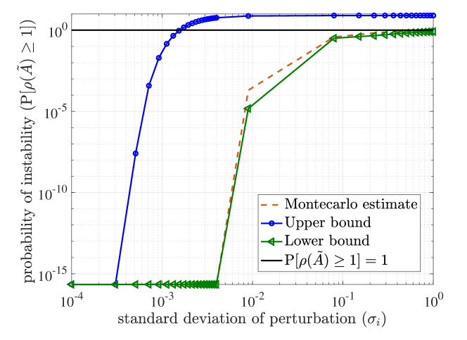
Figure 1: This figure shows the estimate of probability of instability (orange dashed line) of perturbed the closed-loop system described in (8), and the upper and lower bound (blue circle and green triangle, respectively) derived in Theorem 3.3 as a function of perturbation variance ($\sigma_{i}$). Any value less than that of machine epsilon is rounded to that value $(2.2\mathrm{e}-16)$ Notice that (i) the probability of instability lies within the theoretical bounds derived in Theorem 3.3, (ii) the upper (resp. lower) bound converges to zero (resp. one) as the perturbation variance decreases (resp. increases) (iii) the lower bound is tight for all values of $\sigma_{i}$; however, the upper bound proves to be meaningful only when $\sigma_{i}\in(1\mathrm{e}-4,1.5\mathrm{e}-3)$.

4 Illustrative examples

In this section we provide examples to illustrate the bounds derived in Theorem 3.3. To this aim, we consider a simplified discrete-time linear time-invariant model of a vehicle (Dean et al., 2019):

$$x(t+1)=\begin{bmatrix}1&T_{s}&0&0\\ 0&1&0&0\\ 0&0&1&T_{s}\\ 0&0&0&1\end{bmatrix}x(t)+\begin{bmatrix}0&0\\ T_{s}&0\\ 0&0\\ 0&T_{s}\end{bmatrix}u(t),$$ (8)

where $x(t)\in\mathbb{R}^{4}$ contains the vehicle’s position and velocity in cartesian coordinates, $u(t)\in\mathbb{R}^{2}$ is the input signal, and $T_{s}=0.1$ is the sampling time. We assume that the matrices in (8) are unknown, and collect the state trajectory resulting from a single control experiment with a random control input of length $T=500$, which implies that $\mathrm{vec}(X)\in\mathbb{R}^{2000}$. Then, we use the data-driven characterization provided in (Persis and Tesi, 2019, Theorem 3) as a procedure to design a minimum-norm stabilizing controller for (8). We let the experimental data be perturbed at $50$ random locations in $\mathrm{vec}(X)$, that is, $|\mathrm{supp}(Z)|=50$, and compute the Montecarlo estimate of the probability of instability (numerically, over $10000$ instances) of the closed-loop system for different values of the variance of the Gaussian perturbation (with zero mean). Our results are in Fig. 1. We remark that the Jacobian of the data-driven control algorithm ($J_{X}$ in (3)), and thus the matrices $J_{i}$ in (5), can be computed numerically using the available training data, similarly to the numerical computation of the derivative of a scalar function. We refer the reader to Su et al. (2017).

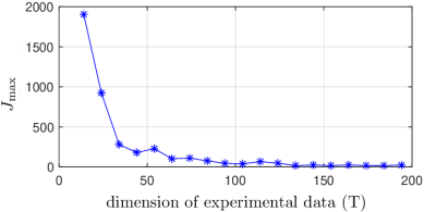
Figure 2: For the setup in Section 4, this figure shows the norm ${J}_{\textup{max}}$ in (7) as a function of the dimension of the experimental data (average over $15$ trials). The norm ${J}_{\textup{max}}$ is a decreasing function of the dimension of the training data, which ensures robustness when the dimension of the experimental data grows faster than the dimension of the compromised data.

To conclude, in Fig. 2 we show that the Jacobian matrix $J_{X}$ of the considered data-driven control algorithm satisfies the bound in (7). That is, the sensitivity of the algorithm in (Persis and Tesi, 2019, Theorem 3) to variations of the training data decreases with the dimension of the training data. This ensures that localized perturbations have increasingly less effect on the final feedback controller, and that the stability of the perturbed closed-loop system is maintained with higher probability. We leave the analytical characterization of this property as the subject of ongoing and future investigation.

5 Conclusion

In this paper we describe a novel framework to quantify the robustness of data-driven control algorithms for linear systems against stochastic perturbations of the training data. We derive lower and upper bounds for the probability of the spectral radius of the closed-loop system exceeding one, as a function of the perturbation statistics, sensitivity of the data-driven algorithm, and properties of the nominal closed-loop system. We also characterize the rate at which the probability of stability of the closed-loop system decreases with the cardinality of the compromised data, and show that such rate is independent of the system dimension. We discuss the qualitative implications of our bounds, and show their effectiveness through numerical simulations. Directions of future research include the derivation of tighter bounds, especially upper bounds since our estimate becomes increasingly more loose with the system dimension, the generalization to more complex algorithms and perturbation models, and the analysis of the sensitivity properties of different data-driven control algorithms.

References

- Baggio et al. (2019) G. Baggio, V. Katewa, and F. Pasqualetti. Data-driven minimum-energy controls for linear systems. IEEE Control Systems Letters, 3(3):589–594, 2019.
- Bharucha-Reid (1973) A.T. Bharucha-Reid. Random Integral Equations. Academic Press, New York, 1973.
- Boucheron et al. (2013) S. Boucheron, G. Lugosi, and P. Massart. Concentration Inequalities: A Nonasymptotic Theory of Independence. Oxford University Press, 2013.
- Dean et al. (2019) S. Dean, N. Matni, B. Recht, and V. Ye. Robust guarantees for perception-based control. arXiv preprint arXiv:1907.03680, 2019.
- Kollo and von Rosen (2005) T. Kollo and D. von Rosen. Advanced Multivariate Statistics with Matrices. Mathematics and Its Applications. Springer, Berlin, 2005.
- Leone et al. (1961) F. C. Leone, L. S. Nelson, and R. B. Nottingham. The folded normal distribution. Technometrics, 3(4):543–550, 1961.
- Makdah et al. (2019) A. A. A. Makdah, V. Katewa, and F. Pasqualetti. A fundamental performance limitation for adversarial classification. IEEE Control Systems Letters, 4(1):169–174, 2019.
- Makdah et al. (2020) A. A. A. Makdah, V. Katewa, and F. Pasqualetti. Accuracy prevents robustness in perception-based control. In American Control Conference, Denver, CO, USA, July 2020.
- Pasqualetti et al. (2013) F. Pasqualetti, F. Dörfler, and F. Bullo. Attack detection and identification in cyber-physical systems. IEEE Transactions on Automatic Control, 58(11):2715–2729, 2013.
- Persis and Tesi (2019) C. De Persis and P. Tesi. Formulas for data-driven control: Stabilization, optimality and robustness. arXiv preprint arXiv:1903.06842, 2019.
- Poland et al. (2018) K. Poland, M. P. McKay, D. Bruce, and E. Becic. Fatal crash between a car operating with automated control systems and a tractor-semitrailer truck. Traffic injury prevention, 19(sup2):S153–S156, 2018.
- Recht (2018) B. Recht. A tour of reinforcement learning: The view from continuous control. Annual Review of Control, Robotics, and Autonomous Systems, 2018.
- Stewart and Ji-guang Sun (1990) G. W. Stewart and Ji-guang Sun. Matrix Perturbation Theory. Computer science and scientific computing. Academic Press, Boston, 1990.
- Su et al. (2017) M. C. Su, Y. Z. Hsieh, C. H. Wang, and P. C. Wang. A jacobian matrix-based learning machine and its applications in medical diagnosis. IEEE Access, 5:20036–20045, 2017.
- Sundaram and Hadjicostis (2011) S. Sundaram and C. Hadjicostis. Distributed function calculation via linear iterative strategies in the presence of malicious agents. IEEE Transactions on Automatic Control, 56(7):1495–1508, 2011.
- Tabuada et al. (2017) P. Tabuada, W.L. Ma, J. Grizzle, and A. D. Ames. Data-driven control for feedback linearizable single-input systems. In IEEE Conf. on Decision and Control, pages 6265–6270, Melbourne, Australia, December 2017.
- Trefethen and Embree (2005) L. N. Trefethen and M. Embree. Spectra and Pseudospectra: the Behavior of Nonnormal Matrices and Operators. Princeton University Press, 2005.
- Tropp (2015) J. A. Tropp. An introduction to matrix concentration inequalities. Foundations and Trends® in Machine Learning, 8(1-2):1–230, 2015.
- Valadbeigi et al. (2019) A. P. Valadbeigi, A. K. Sedigh, and F. L. Lewis. static output-feedback control design for discrete-time systems using reinforcement learning. IEEE transactions on neural networks and learning systems, 2019. To appear.