Rapidity dependence of global polarization in heavy ion collisions

Abstract

We use a geometric model for the hadron polarization with an emphasis on the rapidity dependence. It is based on the model of Brodsky, Gunion, and Kuhn and that of the Bjorken scaling. We make predictions for the rapidity dependence of the hadron polarization in the collision energy range 7.7-200 GeV by taking a few assumed forms of the parameters. The predictions can be tested by future experiments.

I Introduction

In non-central collisions of heavy ions at high energies a huge orbital angular momentum (OAM) is generated. Through spin-orbit couplings in parton-parton scatterings, hadrons can be globally polarized along the OAM of two colliding nuclei Liang and Wang (2005a, b); Voloshin (2004). In a hydrodynamic picture, the huge OAM is distributed into a fluid of quarks and gluons in the form of local vorticity Betz et al. (2007); Becattini et al. (2008, 2015); Pang et al. (2016); Deng and Huang (2016); Jiang et al. (2016), which leads to the local polarization of hadrons along the vorticity direction Becattini et al. (2013); Fang et al. (2016) (for a recent review of the subject, see, e.g., Wang (2017)).

The global polarization of $\Lambda$ and $\bar{\Lambda}$ has been measured in the STAR experiment in Au+Au collisions in the collision energy range 7.7-200 GeV Adamczyk et al. (2017a); Adam et al. (2018) through their weak decays into pions and protons. The magnitude of the global polarization is about a few percent and decreases with increasing collision energies. Hydrodynamic and transport models have been proposed to describe the polarization data for $\Lambda$ and $\bar{\Lambda}$ from which the vorticity fields can be determined Baznat et al. (2013); Csernai et al. (2013, 2014); Teryaev and Usubov (2015); Jiang et al. (2016); Deng and Huang (2016); Ivanov and Soldatov (2017); Li et al. (2017); Wei et al. (2019). Then, through an integration of the vorticity over the freezeout hyper-surface Becattini et al. (2013); Fang et al. (2016), the global polarization of $\Lambda$ and $\bar{\Lambda}$ is obtained and agrees with the data Karpenko and Becattini (2017); Xie et al. (2017); Li et al. (2017); Sun and Ko (2017); Wei et al. (2019).

The previous STAR measurement of the global polarization is limited to the central rapidity region. How the polarization behaves in the forward rapidity region can shed light on the polarization mechanism. The STAR collaboration are currently working on a series of upgrades in the forward region, which will add calorimetry and charged-particle tracking in the rapidity range $[2.5,4]$, and are expected to collect the data of Au+Au collisions at 200 GeV in 2023. Then $\Lambda$ and $\bar{\Lambda}$ may be constructed in this forward region, allowing for the measurement of their polarization.

In this paper, we will give a geometric model for the hadron polarization with an emphasis on the rapidity dependence. This work is the natural extension of a previous work by some of us Gao et al. (2008). The geometric model is based on the model of Brodsky, Gunion, and Kuhn (BGK) Brodsky et al. (1977) and that of the Bjorken scaling Gao et al. (2008). The BGK model can give a good description of the hadron’s rapidity distribution in nucleus-nucleus collisions.

The paper is organized as follows. In Sect. II, we give formulas for the average longitudinal momentum and local orbital angular momentum using the method of Ref. Gao et al. (2008) where the rapidity distribution of hadrons is given by the BGK model. In Sect. III, we use the hard sphere and Woods-Saxon model for the nuclear density distribution to calculate the rapidity distribution of hadrons. In Sect. IV, the hadron polarization from the local orbital angular momentum is calculated with the WS nuclear density distribution. By constraining the parameter by the polarization data at mid-rapidity, we make predictions of the polarization in the forward rapidity region. The summary is given in the last section.

II Average longitudinal momentum and local orbital angular momentum

There is an intrinsic rotation of the initially produced matter in the reaction plane in non-central heavy ion collisions. The rotation can be characterized by tilted local rapidity distribution of produced hadrons toward the projectile and target direction in the transverse plane. We consider non-central collisions of two nuclei $A+A$: the first one is regarded as the projectile moving in $z$ direction while the second is regarded as the target moving in $-z$ direction, see Fig. 1 for illustration. The impact parameter is in the direction from the target to the projectile, i.e. in $x$ direction. The orbital angular momentum (OAM) is in the direction that is determined by the vector product of the impact parameter and the projectile momentum, $\mathbf{b}\times\mathbf{p}_{\mathrm{proj}}$ which is $-y$ direction.

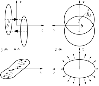
Figure 1: The schematic figure taken from Gao et al. (2008) for non-central heavy ion collisions with impact parameter $\mathbf{b}$ pointing to $x$ direction. The orbital angular momentum is in $-y$ direction.

In the center of the rapidity frame of $\mathrm{p}+A$ collisions, the proton has rapidity $Y_{L}$ and interacts at a transverse impact parameter $\mathbf{r}_{T}$ with $N_{\mathrm{Part}}^{A}\approx\sigma_{NN}T_{A}(\mathbf{r}_{T})$ nucleons with rapidity $-Y_{L}$, where $T_{A}(\mathbf{r}_{T})$ is the thickness function or the number of nucleons per unit area

$$T_{A}(\mathbf{r}_{T})=\int dz\rho_{A}(\mathbf{r}),$$ (1)

with $\mathbf{r}=(x,y,z)$, $\mathbf{r}_{T}=(x,y)$, $\rho_{A}$ is the number density of nucleons in the nucleus, $\sigma_{NN}$ is the inelastic cross section of nucleon-nucleon collisions, and $Y_{L}\approx\ln[\sqrt{s}/(2m_{N})]$ is the largest rapidity. The trangular rapidity distribution of hadrons is the result of string fragmentation between the projectile proton and the target nucleus. The hadrons produced by the wounded projectile proton are in the rapidity range $Y\in[0,Y_{L}]$, while those produced by the wounded target nucleons are in the range $Y\in[-Y_{L},0]$. The rapidity distribution of produced hadrons is approximately given by the BGK model Brodsky et al. (1977) as

$$\frac{d^{3}N_{\mathrm{p}A}}{d^{2}\mathbf{r}_{T}dY} = \frac{dN_{\mathrm{pp}}}{dY}\left[T_{A}(\mathbf{r}_{T})\frac{Y_{L}-Y}{2Y_{L}}+T_{\mathrm{p}}\frac{Y_{L}+Y}{2Y_{L}}\right],$$ (2)

where $T_{\mathrm{p}}\approx 1$ is the number of projectile protons per unit area. In the forward or projectile region $Y\approx Y_{L}$ the rapidity distribution approaches that of p+p collisions $dN_{\mathrm{pp}}/dY$, while in the backward or target region it approaches $(dN_{\mathrm{pp}}/dY)T_{A}(\mathbf{r}_{T})$. From experimental data we take a Gaussian form for $dN_{\mathrm{pp}}/dY$,

$$\frac{dN_{\mathrm{pp}}}{dY}=a_{1}\,\exp\left(-\frac{Y^{2}}{a_{2}}\right)\frac{1}{\sqrt{1+a_{3}(\cosh Y)^{4}}},$$ (3)

where $a_{1}$, $a_{2}$, $a_{3}$ are parameters. The values of these parameters in inelastic non-diffractive events in p+p collisions at some collision energies are determined from the simulation of PYTHIA8.2 Sjostrand et al. (2015) and are listed in Table 1.

Table 1: The values of parameters in the hadron rapidity distribution in inelastic non-diffractive events in p+p collisions at various collision energies from the simulation of PYTHIA8.2 Sjostrand et al. (2015).

$\sqrt{s_{NN}}$ (GeV)	200	130	62.4	54.4	39
$a_{1}$	4.584	4.096	3.862	3.726	3.420
$a_{2}$	26.112	25.896	18.911	18.931	18.779
$a_{3}$	9.70$\times 10^{-8}$	5.61$\times 10^{-7}$	9.75$\times 10^{-6}$	1.71$\times 10^{-5}$	6.61$\times 10^{-5}$

$\sqrt{s_{NN}}$ (GeV)	27	19.6	14.5	11.5	7.7
$a_{1}$	3.421	3.099	3.049	2.784	2.831
$a_{2}$	13.555	13.629	9.947	10.488	8.008
$a_{3}$	2.50$\times 10^{-4}$	8.76$\times 10^{-4}$	2.44$\times 10^{-3}$	5.90$\times 10^{-3}$	9.40$\times 10^{-3}$

Such a trapezoidal shape of the rapidity distribution in (2) in the BGK model is a consequence of the string fragmentation and can be described naturally by the LUND string Andersson et al. (1987) and HIJING model Wang and Gyulassy (1991); Gyulassy and Wang (1994). An extension of the BGK model has been applied to the jet tomography of twisted strongly-coupled quark-qluon plasmas Adil and Gyulassy (2005) as well as the global polarization in nucleus-nucleus collisions Betz et al. (2007). In nucleus-nucleus collisions with projectile $A$ and target $B$, at the point $\mathbf{r}_{T}=(x,y)$ in the transverse plane in the participant region (the coordinate system is shown in the upper-left of Fig. 1), the rapidity distribution of produced hadrons has the form which is a generalization of Eq. (2), i.e. the sum over contributions from projectile (’proj’) and target (’tar’)

$$\frac{d^{3}N_{AB}}{d^{2}\mathbf{r}_{T}dY} = \frac{d^{3}N_{A}^{\mathrm{proj}}}{d^{2}\mathbf{r}_{T}dY}+\frac{d^{3}N_{B}^{\mathrm{tar}}}{d^{2}\mathbf{r}_{T}dY}$$ (4)

$$= \frac{dN_{\mathrm{pp}}}{dY}\left[T_{A}(\mathbf{r}_{T}-\mathbf{b}/2)\frac{Y_{L}+Y}{2Y_{L}}+T_{B}(\mathbf{r}_{T}+\mathbf{b}/2)\frac{Y_{L}-Y}{2Y_{L}}\right].$$

Here, thickness functions $T_{A}(\mathbf{r}_{T}-\mathbf{b}/2)$ and $T_{B}(\mathbf{r}_{T}+\mathbf{b}/2)$ in Eq. (4) are given by

$$T_{A,B}(\mathbf{r}_{T}\mp\mathbf{b}/2) = \int dz\rho^{A,B}(\mathbf{r}_{T}\mp\mathbf{b}/2),$$ (5)

where $\rho^{A,B}(\mathbf{r}_{T}\mp\mathbf{b}/2)$ the participant nucleon number density functions of nuclei $A$ and $B$. One can check that the distribution (4) is proportional to $T_{A/B}(\mathbf{r}_{T}\mp\mathbf{b}/2)$ at the $Y=\pm Y_{L}$.

From Eq. (4) we can derive the distribution in the in-plane position $x$ and the rapidity $Y$ by integrating over the out-plane position $y$ in the range $[-y_{m},y_{m}]$,

$$\frac{d^{2}N_{AB}}{dxdY} = \frac{dN_{\mathrm{pp}}}{dY}\left\{\frac{1}{2}\int_{-y_{m}}^{y_{m}}dy\left[T_{A}(\mathbf{r}_{T}-\mathbf{b}/2)+T_{B}(\mathbf{r}_{T}+\mathbf{b}/2)\right]\right.$$ (6)

$$\left.+\frac{Y}{2Y_{L}}\int_{-y_{m}}^{y_{m}}dy\left[T_{A}(\mathbf{r}_{T}-\mathbf{b}/2)-T_{B}(\mathbf{r}_{T}+\mathbf{b}/2)\right]\right\},$$

where $y_{m}$ is the maximum of $y$ at a specific $x$, in the hard sphere model of the nuclear density distribution it is defined by the boundary of the overlapping region of two nuclei, while in the Woods-Saxon model there is no sharp boundary but it can be set to a value much larger than $y_{m}$ in the hard sphere model. We define the normalized probability distribution of $Y$ at $x$,

$$f(Y,x) = \left(\frac{dN_{AB}}{dx}\right)^{-1}\frac{d^{2}N_{AB}}{dxdY},$$ (7)

where the distribution $dN_{AB}/dx$ is given by

$$\frac{dN_{AB}}{dx} = \int_{-Y_{L}}^{Y_{L}}dY\frac{d^{2}N_{AB}}{dxdY}$$ (8)

$$= \int_{0}^{Y_{L}}dY\frac{dN_{\mathrm{pp}}}{dY}\int_{-y_{m}}^{y_{m}}dy\left[T_{B}(\mathbf{r}_{T}+\mathbf{b}/2)+T_{A}(\mathbf{r}_{T}-\mathbf{b}/2)\right].$$

According to the Bjorken scaling model Gao et al. (2008), the average rapidity of the particle as a function of $Y$ at $x$ in the rapidity window $[Y-\Delta_{Y}/2,Y+\Delta_{Y}/2]$ is given by

$$\left\langle Y\right\rangle_{\Delta} = \frac{\int_{Y-\Delta_{Y}/2}^{Y+\Delta_{Y}/2}dY^{\prime}\>Y^{\prime}f(Y^{\prime},x)}{\int_{Y-\Delta_{Y}/2}^{Y+\Delta_{Y}/2}dY^{\prime}\>f(Y^{\prime},x)}$$ (9)

$$\approx Y+\frac{\Delta_{Y}^{2}}{12}\frac{1}{f(Y,x)}\frac{df(Y,x)}{dY},$$

where $\Delta_{Y}$ is the width of the rapidity window in which particles interact to reach collectivity. We assumed $\Delta_{Y}\ll Y$ so $\Delta_{Y}$ can be treated as a perturbation. The average rapidity of the particle as a function of $x$ in the full rapidity range reads

$$\left\langle Y\right\rangle = \frac{\int_{-Y_{L}}^{Y_{L}}dY\>Yf(Y,x)}{\int_{-Y_{L}}^{Y_{L}}dY\>f(Y,x)}$$ (10)

$$= \frac{1}{Y_{L}}\left\langle Y^{2}\right\rangle_{\mathrm{pp}}\frac{\int_{-y_{m}}^{y_{m}}dy\left[T_{A}(\mathbf{r}_{T}-\mathbf{b}/2)-T_{B}(\mathbf{r}_{T}+\mathbf{b}/2)\right]}{\int_{-y_{m}}^{y_{m}}dy\left[T_{A}(\mathbf{r}_{T}-\mathbf{b}/2)+T_{B}(\mathbf{r}_{T}+\mathbf{b}/2)\right]},$$

where $\left\langle Y^{2}\right\rangle_{\mathrm{pp}}$ is defined as

$$\left\langle Y^{2}\right\rangle_{\mathrm{pp}}=\frac{\int_{-Y_{L}}^{Y_{L}}dY\>(dN_{\mathrm{pp}}/dY)Y^{2}}{\int_{-Y_{L}}^{Y_{L}}dY\>(dN_{\mathrm{pp}}/dY)}.$$ (11)

The average longitudinal momentum $p_{z}$ and the average energy $E_{p}$ of the particle are

$$\left\langle p_{z}\right\rangle = \left\langle p_{T}\right\rangle\sinh\left\langle Y\right\rangle_{\Delta}$$

$$\approx \left\langle p_{T}\right\rangle\sinh Y+\left\langle p_{T}\right\rangle\frac{\Delta_{Y}^{2}}{12}\frac{d\ln f(Y,x)}{dY}\cosh Y,$$

$$\left\langle E_{p}\right\rangle = \left\langle p_{T}\right\rangle\cosh\left\langle Y\right\rangle_{\Delta}$$ (12)

$$\approx \left\langle p_{T}\right\rangle\cosh Y+\left\langle p_{T}\right\rangle\frac{\Delta_{Y}^{2}}{12}\frac{d\ln f(Y,x)}{dY}\sinh Y,$$

where we have treated terms proportional to $\Delta_{Y}^{2}$ as a perturbation. At a given $Y$ we consider two particles located at $x+\Delta x/2$ and $x-\Delta x/2$, in their center of mass frame, the local average OAM for two colliding particles is given by Gao et al. (2008)

$$\left\langle L_{y}\right\rangle \approx -(\Delta x)\left\langle p_{z}^{\mathrm{cm}}\right\rangle$$ (13)

$$\approx -(\Delta x)^{2}\left\langle p_{T}\right\rangle\frac{\Delta_{Y}^{2}}{24}\frac{d\ln f(Y,x)}{dYdx},$$

where $\left\langle p_{z}^{\mathrm{cm}}\right\rangle$ is the average longitudinal momentum in the center of mass frame for one particle. Here $\Delta x$ is a typical impact parameter of particle scatterings. In following sections we will use the average of $d\ln f(Y,x)/dxdY$ over the in-plane coordinate

$$\left\langle\frac{d\ln f(Y,x)}{dYdx}\right\rangle=\frac{\int dx(dN_{AB}/dxdY)(d\ln f(Y,x)/dYdx)}{\int dx(dN_{AB}/dxdY)},$$ (14)

where $dN_{AB}/dxdY$ is given in Eq. (6) as a weight function.

III Rapidity distributions of hadrons in hard sphere and Woods-Saxon model

In this section we will calculate the rapidity distributions for hadrons $f(Y,x)$ in Eq. (7) with the hard sphere (HS) and Woods-Saxon (WS) nuclear density distribution, which are involved in the thickness functions in Eq. (5). As a simple illustration, we consider collisions of two identical nuclei with nucleon number $A$.

III.1 Hard sphere nuclear density distribution

The HS nuclear density is given by

$$\rho_{\mathrm{HS}}(\mathbf{r})=\frac{3A}{4\pi R_{A}^{3}}\theta(R_{A}-r),$$ (15)

where $R_{A}=1.2A^{1/3}$ fm is the nucleus radius. The thickness functions have the analytical form

$$T_{A}(\mathbf{r}_{T}\pm\mathbf{b}/2) = \frac{6A}{4\pi R_{A}^{3}}\left[R_{A}^{2}-(x\pm b/2)^{2}-y^{2}\right]^{1/2}.$$ (16)

Inserting the above into Eq. (4), we obtain the hadron distribution $dN_{AA}/(dxdydY)$, whose numerical results are shown in Fig. 2 at three rapidity values in Au+Au collisions at $\sqrt{s_{NN}}=200$ GeV with the impact parameter $b=1.2R_{A}$. In the HS model, the overlapping region of two nuclei is limited by $|x|<R_{A}-b/2$ and $|y|<\sqrt{R_{A}^{2}-(|x|+b/2)^{2}}$. We see that the distribution at $Y=0$ is symmetric in $x$ and $y$ while that the distribution in the forward (backward) rapidity is shifted to the right (left) in $x$ direction.

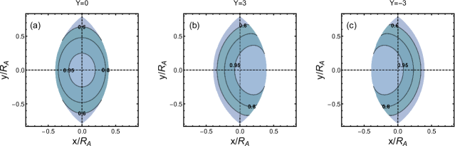
Figure 2: The hadron distributions (contour plot) in the HS model in the transverse plane for Au+Au collisions at $\sqrt{s_{NN}}=200$ GeV and $b=1.2R_{A}$. The number on the contour line denotes the value on the line normalized by that at the origin. The rapidity values are chosen to be $Y=0$ (central), $Y=3$ (forward) and $Y=-3$ (backward).

Integrating over the out-plane coordinate $y$, we obtain the hadron distribution function

$$\frac{d^{2}N_{AA}}{dxdY}=\frac{6A}{4\pi R_{A}^{3}}\frac{dN_{pp}}{dY}\left[C_{1}^{+}+C_{1}^{-}+\frac{Y}{Y_{L}}\left(C_{1}^{+}-C_{1}^{-}\right)\right],$$ (17)

where $C_{1}^{\pm}$ are defined in Eq. (26). In Fig. 3(a), we show $dN_{AA}/dxdY$ as functions of in-plane coordinate $x$ at various rapidity values. We see that the distribution at $Y=0$ is symmetric while the distribution at forward (backward) rapidity is shifted to the positive (negative) $x$. The magnitude of the shift increases slightly with the rapidity. In Fig. 3(b), we show $dN_{AA}/dxdY$ as functions of the rapidity at different $x$. We see that the distribution at $x=0$ is symmetric while that at positive (negative) $x$ is tilted to the forward (backward) rapidity. From Eq. (7), we obtain the normalized function $f(Y,x)$ as

$$f(Y,x) = \frac{dN_{\mathrm{pp}}/dY}{2\int_{0}^{Y_{L}}dY(dN_{\mathrm{pp}}/dY)}\left(1+\frac{Y}{Y_{L}}\cdot\frac{C_{1}^{+}-C_{1}^{-}}{C_{1}^{+}+C_{1}^{-}}\right),$$ (18)

where $|x|\leq R_{A}-b/2$ and $b\leq 2R_{A}$. The numeical results of $f(Y,x)$ are shown in Fig. 3(c,d).

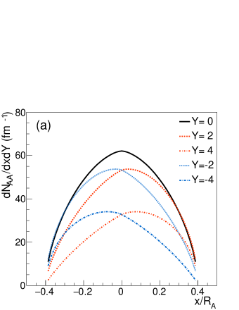
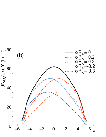
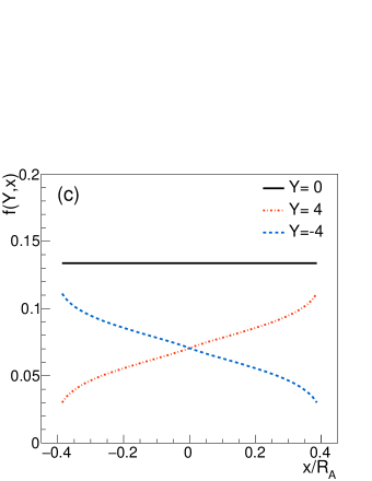
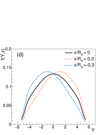
Figure 3: The hadron distributions in the HS model in Au+Au collisions at $\sqrt{s_{NN}}=200$ GeV as functions of (a) the in-plane position $x$ at different rapidity values and as functions of (b) the rapidity $Y$ at different values of $x$. The impact parameter is set to $b=1.2R_{A}$. (c) The normalized distribution $f(Y,x)$ as functions of $x$ at different $Y$. (d) The normalized distribution $f(Y,x)$ corresponding to (b). The definition of $f(Y,x)$ is given in Eq. (18).

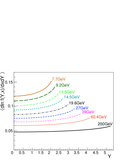
Figure 4: The average quantity $\left\langle d\ln f(Y,x)/dYdx\right\rangle$ as functions of the rapidity $Y$ in the HS model for Au+Au collisions at various collision energies. The impact parameter is set to $b=1.2R_{A}$.

The derivative of $\ln f(Y,x)$ with respect to $Y$ and $x$ is derived in Eq. (35), from which one can obtain $\left\langle d\ln f(Y,x)/dxdY\right\rangle$ through Eq. (14). We show the numerical results of $\left\langle d\ln f(Y,x)/dxdY\right\rangle$ in Fig. 4 as rapidity functions in Au+Au collisions at various collision energies. We see that $\left\langle d\ln f(Y,x)/dYdx\right\rangle$ increases slowly with the rapidity via the $Y/Y_{L}$ term which can be seen in Eq. (35). The relatively obvious increase in the forward rapidity region is an artifact of the HS model in comparison with the WS model in the next subsection. The energy dependence of $\left\langle d\ln f(Y,x)/dYdx\right\rangle$ is mainly controlled by $Y_{L}\approx\ln[\sqrt{s}/(2m_{N})]$ as shown in Eq. (35).

From Eq. (10) we obtain the average rapidity in the full rapidity range as

$$\left\langle Y\right\rangle = \frac{1}{Y_{L}}\left\langle Y^{2}\right\rangle_{\mathrm{pp}}\frac{C_{1}^{+}-C_{1}^{-}}{C_{1}^{+}+C_{1}^{-}}.$$ (19)

The numerical result of the above average rapidity is shown in Fig. 5 which is consistent with Fig. 5 of Ref. Gao et al. (2008).

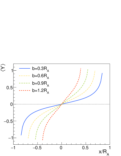
Figure 5: The average rapidity in the full rapidity range for Au+Au collisions at $\sqrt{s_{NN}}=200$ GeV as functions of $x$ from Eq. (19) in the HS model.

III.2 Woods-Saxon nuclear density distribution

In this subsection we choose a more realistic nuclear density distribution, the WS distribution, defined as

$$f_{\mathrm{WS}}(\mathbf{r})=\frac{C_{0}}{\exp\left[\left(r-R_{A}\right)/a\right]+1},$$ (20)

where $r=|\mathbf{r}|$, $a=0.54$ fm, and $C_{0}$ is a normalization constant to make the volume integral of $f_{\mathrm{WS}}(\mathbf{r})$ to be the number of nucleons in the nucleus,

$$C_{0}=\frac{A}{4\pi}\left[\int_{0}^{\infty}drr^{2}\frac{1}{\exp[(r-R_{A})/a]+1}\right]^{-1}.$$ (21)

For Au-197 nuclei, we have $R_{A}\approx 6.98$ fm, $C_{0}\approx A/(4\pi)/120.2\approx 0.131\>\mathrm{fm}^{-3}$. According to the Glauber model, the participant nucleon number density for two colliding nuclei are given by

$$\rho_{\mathrm{WS}}^{A,B}(\mathbf{r}_{T}\mp\mathbf{b}/2) = f_{\mathrm{WS}}^{A,B}(\mathbf{r}_{T}\mp\mathbf{b}/2)$$ (22)

$$\times\left\{1-\exp\left[-\sigma_{NN}\int dzf_{\mathrm{WS}}^{B,A}(\mathbf{r}_{T}\pm\mathbf{b}/2)\right]\right\},$$

where $\sigma_{NN}$ can be taken as the inelastic pp collision cross section.

We consider collisions of two identical nuclei. With the WS distribution in Eq. (20), we can calculate $f(Y,x)$ in Eq. (7). From Eq. (5), the thickness functions become

$$T_{A}(\mathbf{r}_{T}\pm\mathbf{b}/2) = \int_{-\infty}^{\infty}dz\rho_{\mathrm{WS}}^{A}(\mathbf{r}_{T}\pm\mathbf{b}/2)$$ (23)

$$= \int_{-\infty}^{\infty}dzf_{\mathrm{WS}}(\mathbf{r}_{T}\pm\mathbf{b}/2)$$

$$\times\left\{1-\exp\left[-\sigma_{NN}\int dzf_{\mathrm{WS}}(\mathbf{r}_{T}\mp\mathbf{b}/2)\right]\right\}.$$

Substituting Eq. (23) into Eq. (4) and (6), we obtain the hadron distribution $dN_{AA}/(dxdydY)$ in $xy$ plane and $dN_{AA}/(dxdY)$ by an integration over $y$, respectively. The numerical results for $dN_{AA}/(dxdydY)$ and $dN_{AA}/(dxdY)$ are shown in Fig. 6 and 7 respectively for different rapidity values in Au+Au collisions at 200 GeV with $b=1.2R_{A}$. Similar to results of the HS model in Fig. 2 and (3), in the forward/backward rapidity region, the hadron distributions are tilted toward the positive/negative $x$. But different from results of the HS model, the hadron distributions in the WS model are smooth in the edge of the overlapping region.

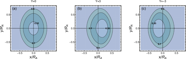
Figure 6: The hadron distributions (contour plot) in the WS model in the transverse plane for Au+Au collisions at $\sqrt{s_{NN}}=200$ GeV and $b=1.2R_{A}$. The number on the contour line denotes the value on the line normalized by that at the origin. The rapidity values are chosen to be $Y=0$ (central), $Y=3$ (forward) and $Y=-3$ (backward).

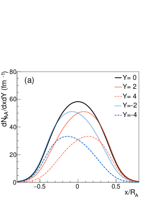
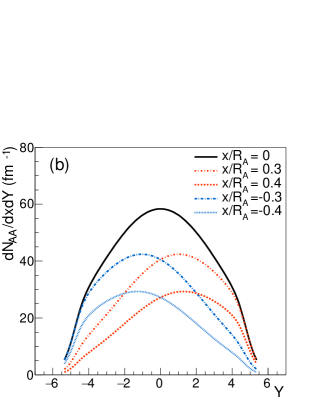
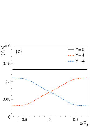
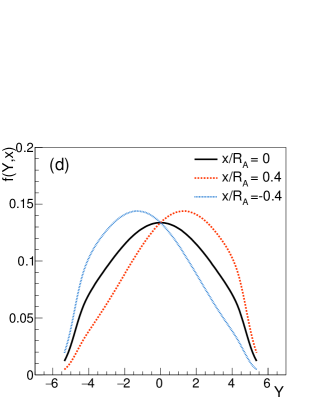
Figure 7: The hadron distributions in the WS model in Au+Au collisions at $\sqrt{s_{NN}}=200$ GeV as functions of (a) the in-plane position $x$ at different rapidity values and as functions of (b) the rapidity $Y$ at different values of $x$. The impact parameter is set to $b=1.2R_{A}$. (c) The normalized distribution $f(Y,x)$ as functions of $x$ at different $Y$. (d) The normalized distribution $f(Y,x)$ corresponding to (b). The definition of $f(Y,x)$ is given in Eq. (7).

We show in Fig. 8 the numerical results for $\left\langle d\ln f(Y,x)/dYdx\right\rangle$ applying Eq. (14) to the WS model. We choose $b=1.2R_{A}$ in Au+Au collisions at different collision energies. We choose $\sigma_{NN}$ as the inelastic proton-proton cross section determined by the global fit of the experimental data Olive et al. (2014), whose values are listed in Table 2. Also shown in Table 2 are the values of $\left\langle d\ln f(Y,x)/dYdx\right\rangle$ at $Y=0$ in Au+Au collisions with the HS and WS distribution.

Table 2: The inelastic nucleon-nucleon cross section $\sigma_{NN}$ at different collisions energies (first two rows). The numerical results of $\left\langle d\ln f(Y,x)/dYdx\right\rangle$ at $Y=0$ in Au+Au collisions at different collisions energies (last two rows). The impact parameter is set to $b=1.2R_{A}$ corresponding to 20-50% centrality in experiments.

$\sqrt{s_{NN}}$(GeV)	200	62.4	54.4	39	27	19.6	14.5	11.5	9.2	7.7
$\sigma_{NN}$(mb)	42.0	36.3	35.2	33.6	32.8	32.3	31.8	31.4	30.9	30.6
$\left\langle\frac{d\ln f(Y,x)}{dYdx}\right\rangle_{\mathrm{HS}}$	0.0471	0.0602	0.0622	0.0678	0.0753	0.0833	0.0925	0.101	0.111	0.121
$\left\langle\frac{d\ln f(Y,x)}{dYdx}\right\rangle_{\mathrm{WS}}$	0.0374	0.0460	0.0472	0.0507	0.0558	0.0614	0.0678	0.0739	0.0809	0.0876

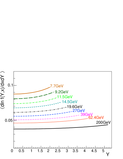
Figure 8: The average quantity $\left\langle d\ln f(Y,x)/dYdx\right\rangle$ as functions of the rapidity $Y$ in the WS model for Au+Au collisions at various collision energies. The impact parameter is set to $b=1.2R_{A}$.

Similar to the results of the HS model, $\left\langle d\ln f(Y,x)/dYdx\right\rangle$ at $Y=0$ increases with decreasing collision energies, and it is a slowly increasing function of $Y$. There are also some differences between the WS and HS results. First, due to the smooth function in the WS model at the edge of the nucleus, the rapidity dependence of $\left\langle d\ln f(Y,x)/dYdx\right\rangle$ in the WS model is slightly weaker than that in the HS model. Second, besides the explicit collision energy dependence of $Y_{L}$, $\sigma_{NN}$ also depends on the collision energy and enters the thickness function via Eq. (22), therefore the increase of $\left\langle d\ln f(Y,x)/dYdx\right\rangle$ at $Y=0$ in the WS model with the decreasing collision energy is slightly slower than in the HS model.

The numerical result for the average rapidity in the full rapidity range from Eq. (10) is shown in Fig. 9 which is consistent with Fig. 5 of Ref. Gao et al. (2008). The difference between Fig. 9 with the WS distribution and Fig. 5 with the HS distribution is that in the edge of the overlapping region of two nuclei $\left\langle Y\right\rangle$ with the WS distribution is smoothly vanishing far outside the overlapping region but $\left\langle Y\right\rangle$ with the HS distribution is discontinuous at the boundary.

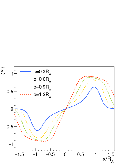
Figure 9: The average rapidity in the full rapidity range for Au+Au collisions $\sqrt{s_{NN}}=200$ GeV as a function of $x$ from Eq. (10) in the WS model.

IV Polarization induced by orbital angular momentum

As proposed in Gao et al. (2008), the OAM in peripheral collisions of two nuclei can induce hadron polarization. Here we assume that the polarization is proportional the local OAM

$$P_{q}\left(Y\right) =\alpha(Y)\left\langle L_{y}\right\rangle$$

$$=-\alpha(Y)(\Delta x)^{2}\frac{\Delta_{Y}^{2}}{24}\left\langle p_{T}\right\rangle\left\langle\frac{d\ln f(Y,x)}{dYdx}\right\rangle,$$ (24)

where we have replaced $d\ln f(Y,x)/dYdx$ in Eq. (13) with its average in Eq. (14), and $\alpha(Y)$ is a rapidity-dependent coefficient. The minus sign means that the polarization is along $-y$ direction. We define a parameter $\kappa(Y)=\alpha(Y)(\Delta x)^{2}\Delta_{Y}^{2}$ as a function of the rapidity $Y$. Note that $\Delta x$, $\Delta_{Y}$ and $\left\langle p_{T}\right\rangle$ can also depend on $Y$ in principle.

The global polarization of $\Lambda$ hyperons at mid-rapidity has been measured in the STAR experiment by which the parameters in Eq. (24) can be determined. At mid-rapidity $Y=0$, Eq. (24) becomes

$$P_{q}(Y=0)=-\frac{1}{24}\kappa_{0}\left\langle p_{T}\right\rangle\left\langle\frac{d\ln f(Y,x)}{dYdx}\right\rangle_{Y=0},$$ (25)

where we have combined three parameters into one $\kappa_{0}\equiv\kappa(0)$. The average transverse momentum $\left\langle p_{T}\right\rangle$ can be determined by kaon data available at some collision energies and an interpolation is made for other collision energies. Results of $\left\langle d\ln f(Y,x)/dYdx\right\rangle_{Y=0}$ are already shown in Table 2.

As our first option, we assume that the parameter $\kappa_{0}$ is a constant of the collision energy whose value is chosen to describe via Eq. (25) the polarization data in the energy range 7.7-62.4 GeV. The results are shown in the left panel of Fig. 10. We see that the collision energy dependence of $P_{q}(Y=0)$ in HS with $\kappa_{0}=6.4$ and that in WS with $\kappa_{0}=8.4$ are roughly consistent with the polarization data in the energy range 7.7-62.4 GeV. But the fitting curves are larger than the data of 200 GeV. Interestingly we find that the energy dependence of our results in both HS and WS model can be well fitted by $\sim 1/Y_{L}$ (dashed line). As our second option, we use the energy dependent $\kappa_{0}$ to fit the data in the energy range 7.7-62.4 GeV including 200 GeV. The results are shown in the right panel of Fig. 10.

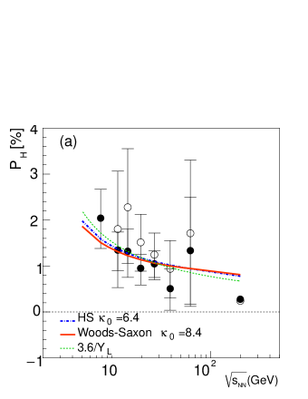
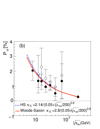
Figure 10: The global polarization of $\Lambda$ and $\bar{\Lambda}$ at mid-rapidity in the HS and WS model in Au+Au collisions at different collision energies. The impact parameter is set to $b=1.2R_{A}$ corresponding to the centrality 20-50%. The STAR data are represented by the solid ($\Lambda$) and open ($\bar{\Lambda}$) circle Adamczyk et al. (2017a); Adam et al. (2018). (a) $\kappa_{0}$ is a contant of the collision energy. (b) $\kappa_{0}$ depends on the collision energy.

Once the values of $\kappa_{0}$ are constrained by the polarization data at mid-rapidity, we can predict the polarization of $\Lambda$ hyperons at larger rapidity. In our prediction we take the WS model and the energy dependent $\kappa_{0}$ as determined in the right panel of Fig. 10. Since we do not know the rapidity dependence of $\kappa(Y)$ and $\left\langle p_{T}\right\rangle$ we will consider three cases and make corresponding prediction for the rapidity dependence of the global polarization: (a) Both $\kappa(Y)=\kappa_{0}$ and $\left\langle p_{T}\right\rangle$ are taken to be constants in rapidity. Therefore the rapidity dependence of the global polarization is solely from $\left\langle d\ln f(Y,x)/dYdx\right\rangle$. (b) Only $\kappa(Y)=\kappa_{0}$ is assumed to be constant in rapidity while $\left\langle p_{T}\right\rangle$ depends on the rapidity. The mid-rapidity values of $\left\langle p_{T}\right\rangle$ are taken from the kaon data in Au+Au collisions in the collision energy range 7.7-200 GeV Abelev et al. (2009); Adamczyk et al. (2017b). The rapidity dependence of $\left\langle p_{T}\right\rangle$ is given by fitting the kaon data in Au+Au collisions at 62.4 GeV and 200 GeV Arsene et al. (2010); Bearden et al. (2005). (c) A rapidity constant $\left\langle p_{T}\right\rangle$ is adopted which takes its value at mid-rapidity at each energy, but the rapidity dependence of $\kappa(Y)$ is assumed to take the form in Eq. (40). (d) Both $\kappa(Y)$ and $\left\langle p_{T}\right\rangle$ depend on the rapidity. The rapidity dependence of $\left\langle p_{T}\right\rangle$ is the same as case (b), while the rapidity dependence of $\kappa(Y)$ is the same as case (c).

Figure 11(a-d) show the polarization results for case (a-d) respectively. In Fig. 11(a) for the constant $\kappa$ and $\left\langle p_{T}\right\rangle$ in rapidity we see that the polarization increases slighly with $Y$ at each collision energy. The positive slope in rapidity (the increase rate of the polarization per unit rapidity) decreases with the collision energy. Figure 11(b) shows the polarization results for the constant $\kappa$ and rapidity dependent $\left\langle p_{T}\right\rangle$. We see that the polarization decreases with $Y$ at each collision energy. At lower energies the decreasing slope (the absolute value of the slope) is larger than that at higher energies. At 200 GeV the polarization is almost a constant of rapidity. In Fig. 11(c) for the rapidity dependent $\kappa$ and constant $\left\langle p_{T}\right\rangle$ in rapidity we see that the polarization increases with rapidity. The lower the collision energy the larger the increasing slope is. The increase trend is stronger than in case (a) and (d) at the same collision energy. Figure 11(d) shows the polarization results for the rapidity dependent $\kappa$ and $\left\langle p_{T}\right\rangle$. At high energies the polarizations increase weakly with rapidity while they are almost contants of rapidity at low energies. Note that the form of $\kappa(Y)$ in Eq. (40) used in case (c) and (d) is valid for $\mu_{B}\lesssim 0.45$ GeV, however, it is beyond such a $\mu_{B}$ limit at 7.7 GeV. Therefore the curves of 7.7 GeV in Figs. 11(c,d) are not shown since they are not reliable.

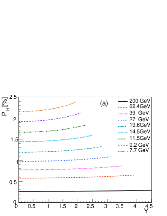
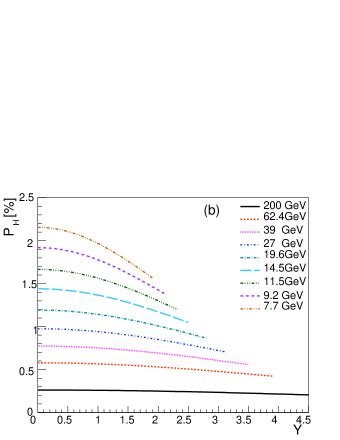
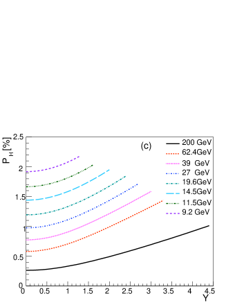
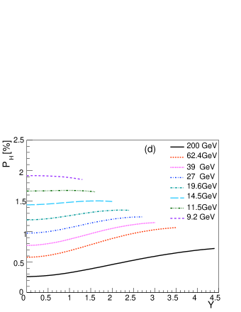
Figure 11: The polarization of $\Lambda$ and $\bar{\Lambda}$ in the WS model as functions of rapidity in Au+Au collisions at different collision energies. We use the collision energy dependent $\kappa_{0}$ as as determined in the right panel of Fig. 10. The impact parameter is set to $b=1.2R_{A}$ corresponding to the centrality 20-50%. The results in case (a), (b), (c) and (d) are presented in panel (a), (b), (c) and (d) respectively.

V Summary

We propose a geometric model for the hadron polarization in heavy ion collisions with an emphasis on the rapidity dependence. It is based on the model of Brodsky, Gunion, and Kuhn and that of the Bjorken scaling Gao et al. (2008). The starting point is the hadron rapidity distribution $d^{3}N_{AA}/d^{2}\mathbf{r}_{T}dY$ as a function of the transverse position $\mathbf{r}_{T}$ in the overlapping region of colliding nuclei and the rapidity $Y$. We use the hard sphere and Woods-Saxon model for the nuclear density distribution from which the thickness function is obtained. The rapidity distribution $d^{3}N_{AA}/dxdY$ depending on the in-plane position $x$ in the overlapping region can be derived from $d^{3}N_{AA}/d^{2}\mathbf{r}_{T}dY$ by integration over the out-plane position $y$. The average rapidity of hadrons can be obtained from the normalized distribution $d^{3}N_{AA}/dxdY$ or $f(Y,x)$. The collective logitudinal momentum $\left\langle p_{z}\right\rangle$ is proportional to $d\ln f(Y,x)/dY$. Then the average local orbital angular momentum $\left\langle L_{y}\right\rangle$ is proportional to the average of $d\ln f(Y,x)/dxdY$ over $x$, which is a function of $Y$. The hadron polarization is assumed to be proportional to $\alpha(Y)\left\langle L_{y}\right\rangle$ with $\alpha(Y)$ is an unknown rapidity function representing a transfer coefficient from the orbital angular momentum in the initial state to the hadron polarization in the final state. There are two parameters in our model that can have rapidity dependence. These parameters at mid-rapidity can be constrained by the polarization data of $\Lambda$ and $\bar{\Lambda}$. Finally we make predictions for the rapidity dependence of the hadron polarization in the collision energy range 7.7-200 GeV by taking a few assumed forms of the parameters. The predictions can be tested by future experiments.

Appendix A Derivation of $d\ln f(Y,x)/dYdx$ for hard sphere distribution

In this Appendix we will derive $d\ln f(Y,x)/dYdx$ in the HS model for the nuclear density distribution from Eq. (17) and (18). The definition of $C_{1}^{\pm}$ and $C_{2}^{\pm}$ are

$$C_{1}^{\pm} =\int_{0}^{y_{m}}dy\left[R_{A}^{2}-(x\mp b/2)^{2}-y^{2}\right]^{1/2},$$ (26)

$$C_{2}^{\pm} =\int_{0}^{y_{m}}dy\left[R_{A}^{2}-(x\mp b/2)^{2}-y^{2}\right]^{-1/2},$$ (27)

where $y_{m}$ is the maximum of $y$ at a fixed $x$

$$y_{m}=\left[R_{A}^{2}-(|x|+b/2)^{2}\right]^{1/2}.$$ (28)

The analytical expressions of $C_{1}^{\pm}$ are

$$C_{1}^{+}\left(x\right)=\begin{cases}\frac{1}{2}\sqrt{R_{A}^{2}-\left(x+b/2\right)^{2}}\sqrt{2bx}+I_{-}(x),&0<x<R_{A}-b/2\\ \frac{\pi}{4}\left[R_{A}^{2}-\left(x-b/2\right)^{2}\right],&-(R_{A}-b/2)<x\leq 0\end{cases}$$ (29)

$$C_{1}^{-}\left(x\right)=\begin{cases}\frac{\pi}{4}\left[R_{A}^{2}-\left(x+b/2\right)^{2}\right],&0\leq x<R_{A}-b/2\\ \frac{1}{2}\sqrt{R_{A}^{2}-\left(x-b/2\right)^{2}}\sqrt{-2bx}+I_{+}(x),&-(R_{A}-b/2)<x<0\end{cases}$$ (30)

where the function $I_{\pm}(x)$ are defined as

$$I_{\pm}(x)=\frac{1}{2}\left[R_{A}^{2}-(x\pm b/2)^{2}\right]\arctan\frac{\sqrt{R_{A}^{2}-\left(x\mp b/2\right)^{2}}}{\sqrt{\mp 2bx}}$$ (31)

The analytical expressions of $C_{2}^{\pm}$ are

$$C_{2}^{+}\left(x\right) =\begin{cases}\arctan\frac{\sqrt{R_{A}^{2}-(x+b/2)^{2}}}{\sqrt{2bx}},&0<x<R_{A}-b/2\\ \frac{\pi}{2},&-(R_{A}-b/2)<x\leq 0\end{cases}$$ (32)

$$C_{2}^{-}\left(x\right) =\begin{cases}\frac{\pi}{2},&0\leq x<R_{A}-b/2\\ \arctan\frac{\sqrt{R_{A}^{2}-(x-b/2)^{2}}}{\sqrt{-2bx}},&-(R_{A}-b/2)<x<0\end{cases}$$ (33)

In terms of $C_{1}^{\pm}$ and $C_{2}^{\pm}$, we obtain the derivative of $\ln f(Y,x)$ with respect to $Y$ as

$$\frac{d\ln f(Y,x)}{dY}=\frac{d\ln(dN_{\mathrm{pp}}/dY)}{dY}+\frac{1}{Y}-\frac{1}{Y}\left\{1+\frac{Y}{Y_{L}}\cdot\frac{C_{1}^{+}-C_{1}^{-}}{C_{1}^{+}+C_{1}^{-}}\right\}^{-1},$$ (34)

and then the derivative of $d\ln f(Y,x)/dY$ with respect to $x$ as

$$\frac{d\ln f(Y,x)}{dYdx} = \frac{1}{Y_{L}}\left[1+\frac{Y}{Y_{L}}\cdot\frac{C_{1}^{+}-C_{1}^{-}}{C_{1}^{+}+C_{1}^{-}}\right]^{-2}\left\{-\frac{x(C_{2}^{+}-C_{2}^{-})-(b/2)(C_{2}^{+}+C_{2}^{-})}{(C_{1}^{+}+C_{1}^{-})}\right.$$ (35)

$$+\frac{(C_{1}^{+}-C_{1}^{-})\left[x(C_{2}^{+}+C_{2}^{-})-(b/2)(C_{2}^{+}-C_{2}^{-})\right]}{(C_{1}^{+}+C_{1}^{-})^{2}}$$

$$-2(2b|x|)^{1/2}(|x|+b/2)\left[R_{A}^{2}-(|x|+b/2)^{2}\right]^{-1/2}$$

$$\times\left.\frac{C_{1}^{+}\theta(-x)+C_{1}^{-}\theta(x)}{(C_{1}^{+}+C_{1}^{-})^{2}}\right\},$$

where we have used

$$\frac{d}{dx}\int_{0}^{a(x)}dyb(x,y) = \int_{0}^{a(x)}dy\frac{\partial b(x,y)}{\partial x}+b(x,a(x))\frac{da(x)}{dx}.$$ (36)

Appendix B Rapidity dependence of $\kappa(Y)$ in case (c) and (d)

There is a similarity in hadron production between the case at forward rapidity but high collision energy and that at central rapidity but lower collision energy. Here the baryon number density or baryon chemical potential is the relevant physical quantity. Therefore, if we neglect the system size effect, we can make an ansatz for $\kappa(Y)$ based on this similarity.

By fitting the data in Fig. 8(b) we find the following energy behavior of $\kappa_{0}\equiv\kappa(Y=0)$,

$$\kappa(Y=0)=\frac{2.8}{\left(0.05+\sqrt{s_{NN}}/200\right)^{0.6}}.$$ (37)

The collision energy dependence of the baryon chemical potential at mid-rapidity can be given by Andronic et al. (2018)

$$\mu_{B}(Y=0)=\frac{1.3075}{1+0.288\sqrt{s_{NN}}}\>\textrm{GeV}.$$ (38)

We can solve $\sqrt{s_{NN}}$ as a function of $\mu_{B}(Y=0)$ and obtain

$$\kappa(Y=0)=\frac{2.8}{\left(0.05+\left(1.3075/\mu_{B}(Y=0)-1\right)/57.6\right)^{0.6}}.$$ (39)

within the range $\mu_{B}\lesssim 0.45$ GeV, i.e., in the collision energy range 7.7-200 GeV. We can generalize the above expression to other rapidity values as

$$\kappa(Y)=\frac{2.8}{\left(0.05+\left(1.3075/\mu_{B}(Y)-1\right)/57.6\right)^{0.6}},$$ (40)

by taking the following parametrization of $\mu_{B}(Y)$ Becattini et al. (2007)

$$\mu_{B}(Y)=\mu_{B}(Y=0)+w\left(\sqrt{s_{NN}}\right)Y^{2},$$ (41)

with the width parameter

$$w\left(\sqrt{s_{NN}}\right)=0.09527-0.01594\log\sqrt{s_{NN}}.$$ (42)

References

- Liang and Wang (2005a) Z.-T. Liang and X.-N. Wang, Phys. Rev. Lett. 94, 102301 (2005a), [Erratum: Phys. Rev. Lett.96,039901(2006)], eprint nucl-th/0410079.
- Liang and Wang (2005b) Z.-T. Liang and X.-N. Wang, Phys. Lett. B629, 20 (2005b), eprint nucl-th/0411101.
- Voloshin (2004) S. A. Voloshin (2004), eprint nucl-th/0410089.
- Betz et al. (2007) B. Betz, M. Gyulassy, and G. Torrieri, Phys. Rev. C76, 044901 (2007), eprint 0708.0035.
- Becattini et al. (2008) F. Becattini, F. Piccinini, and J. Rizzo, Phys. Rev. C77, 024906 (2008), eprint 0711.1253.
- Becattini et al. (2015) F. Becattini, G. Inghirami, V. Rolando, A. Beraudo, L. Del Zanna, A. De Pace, M. Nardi, G. Pagliara, and V. Chandra, Eur. Phys. J. C75, 406 (2015), [Erratum: Eur. Phys. J.C78,no.5,354(2018)], eprint 1501.04468.
- Pang et al. (2016) L.-G. Pang, H. Petersen, Q. Wang, and X.-N. Wang, Phys. Rev. Lett. 117, 192301 (2016), eprint 1605.04024.
- Deng and Huang (2016) W.-T. Deng and X.-G. Huang, Phys. Rev. C93, 064907 (2016), eprint 1603.06117.
- Jiang et al. (2016) Y. Jiang, Z.-W. Lin, and J. Liao, Phys. Rev. C94, 044910 (2016), [Erratum: Phys. Rev.C95,no.4,049904(2017)], eprint 1602.06580.
- Becattini et al. (2013) F. Becattini, V. Chandra, L. Del Zanna, and E. Grossi, Annals Phys. 338, 32 (2013), eprint 1303.3431.
- Fang et al. (2016) R.-H. Fang, L.-G. Pang, Q. Wang, and X.-N. Wang, Phys. Rev. C94, 024904 (2016), eprint 1604.04036.
- Wang (2017) Q. Wang, Nucl. Phys. A967, 225 (2017), eprint 1704.04022.
- Adamczyk et al. (2017a) L. Adamczyk et al. (STAR), Nature 548, 62 (2017a), eprint 1701.06657.
- Adam et al. (2018) J. Adam et al. (STAR), Phys. Rev. C98, 014910 (2018), eprint 1805.04400.
- Baznat et al. (2013) M. Baznat, K. Gudima, A. Sorin, and O. Teryaev, Phys. Rev. C88, 061901 (2013), eprint 1301.7003.
- Csernai et al. (2013) L. P. Csernai, V. K. Magas, and D. J. Wang, Phys. Rev. C87, 034906 (2013), eprint 1302.5310.
- Csernai et al. (2014) L. P. Csernai, D. J. Wang, M. Bleicher, and H. Stoecker, Phys. Rev. C90, 021904 (2014).
- Teryaev and Usubov (2015) O. Teryaev and R. Usubov, Phys. Rev. C92, 014906 (2015).
- Ivanov and Soldatov (2017) Yu. B. Ivanov and A. A. Soldatov, Phys. Rev. C95, 054915 (2017), eprint 1701.01319.
- Li et al. (2017) H. Li, L.-G. Pang, Q. Wang, and X.-L. Xia, Phys. Rev. C96, 054908 (2017), eprint 1704.01507.
- Wei et al. (2019) D.-X. Wei, W.-T. Deng, and X.-G. Huang, Phys. Rev. C99, 014905 (2019), eprint 1810.00151.
- Karpenko and Becattini (2017) I. Karpenko and F. Becattini, Eur. Phys. J. C77, 213 (2017), eprint 1610.04717.
- Xie et al. (2017) Y. Xie, D. Wang, and L. P. Csernai, Phys. Rev. C95, 031901 (2017), eprint 1703.03770.
- Sun and Ko (2017) Y. Sun and C. M. Ko, Phys. Rev. C96, 024906 (2017), eprint 1706.09467.
- Gao et al. (2008) J.-H. Gao, S.-W. Chen, W.-t. Deng, Z.-T. Liang, Q. Wang, and X.-N. Wang, Phys. Rev. C77, 044902 (2008), eprint 0710.2943.
- Brodsky et al. (1977) S. J. Brodsky, J. F. Gunion, and J. H. Kuhn, Phys. Rev. Lett. 39, 1120 (1977).
- Sjostrand et al. (2015) T. Sjostrand, S. Ask, J. R. Christiansen, R. Corke, N. Desai, P. Ilten, S. Mrenna, S. Prestel, C. O. Rasmussen, and P. Z. Skands, Comput. Phys. Commun. 191, 159 (2015), eprint 1410.3012.
- Andersson et al. (1987) B. Andersson, G. Gustafson, and B. Nilsson-Almqvist, Nucl. Phys. B281, 289 (1987).
- Wang and Gyulassy (1991) X.-N. Wang and M. Gyulassy, Phys. Rev. D44, 3501 (1991).
- Gyulassy and Wang (1994) M. Gyulassy and X.-N. Wang, Comput. Phys. Commun. 83, 307 (1994), eprint nucl-th/9502021.
- Adil and Gyulassy (2005) A. Adil and M. Gyulassy, Phys. Rev. C72, 034907 (2005), eprint nucl-th/0505004.
- Olive et al. (2014) K. A. Olive et al. (Particle Data Group), Chin. Phys. C38, 090001 (2014).
- Abelev et al. (2009) B. I. Abelev et al. (STAR), Phys. Rev. C79, 034909 (2009), eprint 0808.2041.
- Adamczyk et al. (2017b) L. Adamczyk et al. (STAR), Phys. Rev. C96, 044904 (2017b), eprint 1701.07065.
- Arsene et al. (2010) I. C. Arsene et al. (BRAHMS), Phys. Lett. B687, 36 (2010), eprint 0911.2586.
- Bearden et al. (2005) I. G. Bearden et al. (BRAHMS), Phys. Rev. Lett. 94, 162301 (2005), eprint nucl-ex/0403050.
- Andronic et al. (2018) A. Andronic, P. Braun-Munzinger, K. Redlich, and J. Stachel, Nature 561, 321 (2018), eprint 1710.09425.
- Becattini et al. (2007) F. Becattini, J. Cleymans, and J. Strumpfer, PoS CPOD07, 012 (2007), eprint 0709.2599.