Abstract

A committee’s decisions on more than two alternatives much depend on the adopted voting method, and so does the distribution of power among the committee members. We investigate how different aggregation methods such as plurality runoff, Borda count, or Copeland rule map asymmetric numbers of seats, shares, voting weights, etc. to influence on outcomes when preferences vary. A generalization of the Penrose-Banzhaf power index is proposed and applied to the IMF Executive Board’s election of a Managing Director, extending a priori voting power analysis from binary simple voting games to choice in weighted committees.

Keywords:

weighted voting $\cdot$ voting power $\cdot$ weighted committee games $\cdot$ plurality runoff $\cdot$ Borda rule $\cdot$ Copeland rule $\cdot$ Schulze rule $\cdot$ IMF Executive Board $\cdot$ IMF Director

We are grateful to Hannu Nurmi for stimulating discussions on the topic. We also benefitted from feedback on seminar or workshop presentations in Bamberg, Bayreuth, Berlin, Bremen, Dagstuhl, Delmenhorst, Graz, Hagen, Hamburg, Hanover, Leipzig, Moscow, Munich and Turku.

1 Introduction

The aggregation of individual preferences by some form of voting is common in politics, business, and everyday life. Members of a board, council, or committee are rarely aware how much their collective choices depend on the adopted aggregation rule. The importance of the method may be identified a posteriori by comparing voting outcomes for a given preference configuration. For instance, suppose a hiring committee involved three groups with $n_{1}=6$, $n_{2}=5$, and $n_{3}=3$ members each and the following preferences over five candidates $\{a,b,c,d,e\}$: $a\succ_{1}d\succ_{1}e\succ_{1}c\succ_{1}b$, $b\succ_{2}c\succ_{2}d\succ_{2}e\succ_{2}a$, and $c\succ_{3}e\succ_{3}d\succ_{3}b\succ_{3}a$. If the groups voted sincerely (for informational, institutional, or other reasons) then candidate $a$ would have received the position under plurality rule with 6 vs. 5 vs. 3 votes. However, requiring a runoff between the front-runners, given that none has majority support, would have made $b$ the winner with 8 to 6 votes. Candidate $c$ would have won every pairwise comparison and been the Condorcet winner; Borda rule would have singled out $d$; candidate $e$ could have been the winner if approval voting had been used.

With enough posterior information, each voter group can identify a ‘most-preferred voting method’ for the decision at hand: group 1 should have tried to impose plurality rule in order to have its way; group 2 should have argued for plurality runoff; and group 3 for pairwise comparisons. It is less obvious, though, how adoption of one aggregation method rather than another will affect a group’s success and influence a priori, i.e., not yet knowing what will be the applicable preferences, or averaged across many decisions. More generally, can we verify if small groups are enjoying a greater say when committees fill a top position, elect an official, etc. by pairwise votes or by the plurality runoff method? Which rules from a given list of suggestions tend to maximize (or minimize) voting power of a particularly sized group in a committee? There is a huge literature on voting power but questions of this kind have to our knowledge not been addressed by it yet. We seek to change this by generalizing tools that were developed for analysis of simple voting games with binary options (‘yes’ or ‘no’) to collective choice from $m\geq 3$ alternatives.

The most prominent tools for analyzing the former are the Penrose-Banzhaf index (Penrose:1946; Banzhaf:1965) and the Shapley-Shubik index [Shapley and ShubikShapley and Shubik1954]. They evaluate the sensitivity of the outcome to changes in a given voter’s preferences – operationalized as the likelihood of this voter being pivotal or critical: flipping its vote would swing the collective decision – under specific probabilistic assumptions. This paper applies the same logic to weighted committee games. These, more simply referred to as weighted committees, are tuples $(N,A,r|\mathbf{w})$ that specify a set $N=\{1,\ldots,n\}$ of players, a set $A=\{a_{1},\ldots,a_{m}\}$ of alternatives, and the combination $r|\mathbf{w}$ of an anonymous voting method $r$ (e.g., Borda rule, plurality rule, and so on) with a vector $\mathbf{w}$ of integers that represents group sizes, voting shares, etc.

As in analysis of (binary) simple voting games, high a priori voting power of player $i\in N$ in a committee goes with high sensitivity of the outcome to $i$’s preferences. It can be quantified as the probability for a change in $i$’s preferences causing a change of the collective choice. Although other assumptions could be made, we focus on the simplest case in which all profiles of strict preference orderings are equally likely a priori. This corresponds to the Penrose-Banzhaf index for $m=2$. The respective power indications help to assess who gains and loses from institutional reforms or whether the distribution of influence in a committee satisfies some fairness criterion; they can also inform stakeholders, lobbyists, or other committee outsiders with an interest in who has how much say in the committee.

2 Related Work

The distribution of power in binary weighted voting games has received wide attention ever since [Ch. 10]vonNeumann/Morgenstern:1953 formalized them as a subclass of so-called simple (voting) games. See, e.g., Mann/Shapley:1962, Riker/Shapley:1968, Owen:1975:presidential, or Brams:1978 for seminal investigations. The binary framework can be restrictive, however. Even for collective ‘yes’-or-‘no’ decisions, individual voters usually have more than two options. For instance they can abstain or not even attend a vote, and this may affect the outcome differently than casting a vote either way. Corresponding situations have been formalized as ternary voting games (Felsenthal/Machover:1997; Tchantcho/DiffoLambo/Pongou/Engoulou:2008; Parker:2012) and quaternary voting games [Laruelle and ValencianoLaruelle and Valenciano2012]. Players can also be allowed to express graded intensities of support: in $(j,k)$-games, studied by Hsiao/Raghavan:1993 and Freixas and Zwicker (Freixas/Zwicker:2003, Freixas/Zwicker:2009), each player selects one of $j$ ordered levels of approval. The resulting $j$-partitions of players are mapped to one of $k$ ordered output levels; suitable power indices have been defined by Freixas (Freixas:2005:Banzhaf, Freixas:2005:Shapley).

Linear orderings of actions and feasible outcomes, as required by $(j,k)$-games, are naturally given in many applications but fail to exist in others. Think of options that have multidimensional attributes – for instance, candidates for office or an open position, policy programs, locations of a facility, etc. Pertinent extensions of simple games, along with corresponding power measures, have been introduced as multicandidate voting games by Bolger:1986 and taken up as simple $r$-games by Amer/Carreras/Magana:1998b and as weighted plurality games by Chua/Ueng/Huang:2002. They require each player to vote for a single candidate. This results in partitions of player set $N$ that, in contrast to $(j,k)$-games, are mapped to a winning candidate without ordering restrictions.

We will draw on the yet more general framework of weighted committee games (Kurz/Mayer/Napel:2018). Winners in these games can depend on the entire preference rankings of voters rather than just the respective top. We conceive of player $i$’s influence or voting power as the sensitivity of joint decisions to $i$’s actions or likings. The resulting ability to affect collective outcomes is closely linked to the opportunity to manipulate social choices in the sense of Gibbard:1973 and Satterthwaite:1975. Our investigation therefore relates to computational studies by Nitzan:1985, Kelly:1993, Aleskerov/Kurbanov:1999, or Smith:1999 that have quantified the aggregate manipulability of a given decision rule. The conceptual difference between corresponding manipulability indices and the power index defined below is that the latter is evaluating consequences of arbitrary preference perturbations, while the indicated studies only look at strategic preference misrepresentation that is beneficial from the perspective of a player’s original preferences. Voting power as we quantify it could be used for a player’s strategic advantage but it need not. A ‘preference change’ might also be purely idiosyncratic, result from log-rolling or external lobbying (where costs of persuasion can relate more to preference intensity than a player’s original ranking of options), or could be a demonstration of power for its own sake.

Other conceptualizations of the influence derived from a given collective choice rule track the sets of outcomes that can be induced by partial coalitions. For instance, Moulin:1981 uses veto functions in order to describe outcomes that given coalitions of players could jointly prevent; Peleg’s Peleg:1984 effectivity functions describe the power structure in a committee by a list of all sets of alternatives that specific coalitions of voters can force the outcome to lie in. We, by contrast, follow the literature pioneered by Penrose:1946, Shapley/Shubik:1954, and Banzhaf:1965, and try to assess individual influence on outcomes concisely by a number between zero and one.

3 Preliminaries

3.1 Anonymous Voting Rules

We consider finite sets $N=\{1,\dots,n\}$ of $n$ voters or players such that each voter $i\in N$ has strict preferences $P_{i}$ over a set $A=\{a_{1},\dots,a_{m}\}$ of $m\geq 2$ alternatives. We write $abc$ in abbreviation of $aP_{i}bP_{i}c$ when the player’s identity is clear. The set of all $m!$ strict preference orderings on $A$ is denoted by $\mathcal{P}(A)$. A (resolute) voting rule $r\colon\mathcal{P}(A)^{n}\to A$ maps each preference profile $\mathbf{P}=(P_{1},\dots,P_{n})$ to a single winning alternative $a^{*}=r(\mathbf{P})$. Rule $r$ is anonymous if for any $\mathbf{P}\in\mathcal{P}(A)$ and any permutation $\pi\colon N\to N$ with $\pi(\mathbf{P})=(P_{\pi(1)},\dots,P_{\pi(n)})$ we have $r(\mathbf{P})=r(\pi(\mathbf{P}))$.

Rule	Winning alternative at preference profile $\mathbf{P}$
Borda	$r^{B}(\mathbf{P})\in\operatorname*{arg\,max}_{a\in A}\sum_{i\in N}b_{i}(a,\mathbf{P})$
Copeland	$r^{C}(\mathbf{P})\in\operatorname*{arg\,max}_{a\in A}\big{|}\{a^{\prime}\in A\ |\ a\succ_{M}^{\mathbf{P}}a^{\prime}\}\big{|}$
Plurality	$r^{P}(\mathbf{P})\in\operatorname*{arg\,max}_{a\in A}\big{|}\{i\in N\ |\ \forall a^{\prime}\neq a\in A\colon aP_{i}a^{\prime}\}\big{|}$
Plurality runoff	$r^{PR}(\mathbf{P})\begin{dcases}=r^{P}(\mathbf{P})\;\text{ if }\;\big{|}\{i\in N\ |\ \forall a^{\prime}\in A\setminus\{r^{P}(\mathbf{P})\}\colon r^{P}(\mathbf{P})P_{i}a^{\prime}\}\big{|}>\tfrac{n}{2}\\ \in\operatorname*{arg\,max}_{a\in\{a_{(1)},a_{(2)}\}}\big{|}\{i\in N\ |\ \forall a^{\prime}\neq a\in\{a_{(1)},a_{(2)}\}\colon aP_{i}a^{\prime}\}\big{|}\text{ otherwise}\end{dcases}$
Schulze	$r^{S}(\mathbf{P})$ – see Schulze:2011

Table 1: Considered anonymous voting rules

We will restrict attention to truthful voting under one of the five anonymous rules summarized in Table 1, assuming lexicographic tie breaking. See Laslier:2012 on the pros and cons of a big variety of voting procedures. Our selection comprises two positional rules (Borda, plurality), two Condorcet methods (Copeland, Schulze), and a two-stage procedure that is used for filling political offices in many European jurisdictions (plurality runoff).

Under plurality rule $r^{P}$, each voter simply names his or her top-ranked alternative and the alternative that is ranked first by the most voters is chosen. This is also the winner under plurality with runoff rule $r^{PR}$ if the obtained plurality constitutes a majority (i.e., more than 50% of votes); otherwise a binary runoff between the alternatives $a_{(1)}$ and $a_{(2)}$ that obtained the highest and second-highest plurality scores in the first stage is conducted.

Borda rule $r^{B}$ has each player $i$ assign $m-1$, $m-2$, …, $0$ points to the alternative that he or she ranks first, second, etc. These points $b_{i}(a,\mathbf{P}):=\big{|}\{a^{\prime}\in A\ |\ aP_{i}a^{\prime}\}\big{|}$ equal the number of alternatives that $i$ ranks below $a$. The alternative with the highest total number of points, known as its Borda score, is selected.

Copeland rule $r^{C}$ considers pairwise majority votes between the alternatives. They define the majority relation $a\succ_{M}^{\mathbf{P}}a^{\prime}\ :\Leftrightarrow\ \big{|}\{i\in N\ |\ aP_{i}a^{\prime}\}\big{|}>\big{|}\{i\in N\ |\ a^{\prime}P_{i}a\}\big{|}$ and the alternative that beats the most others according to $\succ_{M}^{\mathbf{P}}$ is selected. Copeland rule is a Condorcet method: if some alternative $a$ beats all others, then $r^{C}(\mathbf{P})=a$. The same is true for Schulze rule $r^{S}$. But while $r^{C}$ just counts the number of direct pairwise victories, $r^{S}$ also considers indirect victories and invokes majority margins in order to evaluate their strengths. $r^{S}$ then picks the alternative that has the strongest chain of direct or indirect majority support (see Schulze:2011 for details). The attention paid to margins makes $r^{S}$ more sensitive to voting weights than $r^{C}$ in case $\succ_{M}^{\mathbf{P}}$ is cyclical. Despite its non-trivial computation, $r^{S}$ has been applied, e.g., by the Wikimedia Foundation and Linux open-source communities.

3.2 Weighted Committees

Anonymous rules treat any components $P_{i}$ and $P_{j}$ of a preference profile $\mathbf{P}$ like indistinguishable ballots. Still, when a committee conducts pairwise comparisons, plurality voting, etc., two individual preferences often feed into the collective decision rather asymmetrically because, e.g., stockholders have as many votes as they own shares or the relevant players $i\in N$ in a political committee cast bloc votes in proportion to party seats. The resulting (non-anonymous) mapping from preferences to outcomes is a combination of anonymous voting rule $r$ with weights $w_{1},\ldots,w_{n}$ for players $1,\ldots,n$ that is defined for all $\mathbf{P}\in\mathcal{P}(A)^{n}$ by

$$r|\mathbf{w}(\mathbf{P}):=r([P_{1}]^{w_{1}},[P_{2}]^{w_{2}},\ldots,[P_{n}]^{w_{n}})=r(\underbrace{P_{1},\ldots,P_{1}}_{w_{1}\text{ times}},\underbrace{P_{2},\ldots,P_{2}}_{w_{2}\text{ times}},\ldots,\underbrace{P_{n},\ldots,P_{n}}_{w_{n}\text{ times}}).$$ (1)

The combination $(N,A,r|\mathbf{w})$ of a set of voters, a set of alternatives and a particular weighted voting rule defines a weighted committee (game). When the underlying anonymous rule is plurality rule $r^{P}$, then $(N,A,r^{P}|\mathbf{w})$ is called a (weighted) plurality committee. Similarly, $(N,A,r^{PR}|\mathbf{w})$, $(N,A,r^{B}|\mathbf{w})$, $(N,A,r^{C}|\mathbf{w})$ and $(N,A,r^{S}|\mathbf{w})$ are referred to as a plurality runoff committee, Borda committee, Copeland committee, and Schulze committee. See Kurz/Mayer/Napel:2018 on structural differences between them.

Weighted committee games $(N,A,r|\mathbf{w})$ and $(N,A,r^{\prime}|\mathbf{w^{\prime}})$ are equivalent if the respective mappings from preference profiles to outcomes $a^{*}$ coincide; that is, when $r|\mathbf{w}(\mathbf{P})=r^{\prime}|\mathbf{w^{\prime}}(\mathbf{P})$ for all $\mathbf{P}\in\mathcal{P}(A)^{n}$. Equivalent games evidently come with equivalent expectations for individual players to influence the collective decision (voting power) and to obtain outcomes that match their own preferences (success). We will focus on voting power and non-equivalent committees that involve either the same rule $r$ but different weights $\mathbf{w}$ and $\mathbf{w^{\prime}}$, or the same weights $\mathbf{w}$ but different rules $r$ and $r^{\prime}$. Example questions that we would like to address are: to what extent does a change of voting weights, implied for example by the recent re-allocation of voting rights in the International Monetary Fund or party-switching of a member of parliament, shift the respective balance of power? How does players’ attractiveness to lobbyists change when a committee replaces one voting method by another?

4 Measuring Influence in Weighted Committees

Some obvious shortcomings notwithstanding (see, e.g., Garrett/Tsebelis:1999, Garrett/Tsebelis:2001), voting power indices such as the Penrose-Banzhaf and the Shapley-Shubik index have received wide attention in theoretical and applied analysis of binary decisions. See, e.g., the contributions in Holler/Nurmi:2013. Most indices can be seen as operationalizing power of player $i$ as expected sensitivity of collective decisions to player $i$’s behavior [Napel and WidgrénNapel and Widgrén2004]. Sensitivity in the binary case means that, taking the behavior of other players as given, the collective outcome would have been different had player $i$ voted ‘no’ instead of ‘yes’, or ‘yes’ instead of ‘no’. Distinct indices reflect distinct probabilistic assumptions about the voting configurations that are evaluated. For instance, the Penrose-Banzhaf index is predicated on the assumption that the preferences of all $n$ players are independent random variables and the $2^{n}$ different ‘yes’-‘no’ configurations are equally likely.

4.1 Power as (Normalized) Expected Sensitivity of the Outcome

It is not hard to generalize the idea of measuring influence as outcome sensitivity to weighted committees $(N,A,r|\mathbf{w})$. Continuing in the Penrose-Banzhaf tradition, we will assume that individual preferences are drawn independently from the uniform distribution over $\mathcal{P}(A)$, i.e., all profiles $\mathbf{P}\in\mathcal{P}(\{a_{1},\ldots,a_{m}\})^{n}$ are equally likely. In order to assess the voting power of player $i$ with weight $w_{i}$, we perturb $i$’s realized preferences $P_{i}$ to a random $P_{i}^{\prime}\neq P_{i}\in\mathcal{P}(A)$ and check if this individual preference change would change the collective outcome. Specifically, using notation $\mathbf{P}=(P_{i},\mathbf{P}_{-i})$ with $\mathbf{P}_{-i}=(P_{1},\dots,P_{i-1},P_{i+1},\dots,P_{n})$, we are interested in the behavior of indicator function

$$\Delta r|\mathbf{w}(\mathbf{P};{P^{\prime}_{i}}):=\begin{cases}1&\text{if}\quad r|\mathbf{w}(\mathbf{P})\neq r|\mathbf{w}(P_{i}^{\prime},\mathbf{P}_{-i}),\\ 0&\text{if}\quad r|\mathbf{w}(\mathbf{P})=r|\mathbf{w}(P_{i}^{\prime},\mathbf{P}_{-i}).\end{cases}$$ (2)

We stay agnostic about the precise source of perturbations: the switch from $P_{i}$ to $P_{i}^{\prime}$ might reflect a spontaneous change of mind or intentional preference misrepresentation, e.g., because someone has bought $i$’s vote. Variations might also be the result of a mistake or of receiving last-minute private information about some of the candidates. Our important premise is only that: a committee member’s input to the collective decision process matters more, the more influential player $i$ is in the committee and vice versa.

We can then quantify player $i$’s a priori influence or power – and compare it to that of other players or for variations of $r|\mathbf{w}$ – by taking expectations over all $(m!)^{n}$ conceivable $\mathbf{P}$ and all $m!-1$ possible perturbations of $P_{i}$ at any given $\mathbf{P}$:

$$\widehat{\mathcal{I}}_{i}(N,A,r|\mathbf{w}):=\mathbb{E}\big{[}\Delta r|\mathbf{w}(\mathbf{P};{P^{\prime}_{i}})\big{]}=\frac{\sum_{\mathbf{P}\in\mathcal{P}(A)^{n}}\sum_{P_{i}^{\prime}\neq P_{i}\in\mathcal{P}(A)}\Delta r|\mathbf{w}(\mathbf{P};{P^{\prime}_{i}})}{(m!)^{n}\cdot(m!-1)},\;\;i\in N.$$ (3)

A value of $\widehat{\mathcal{I}}_{i}(N,A,r|\mathbf{w})=0.25$, for example, means that 25% of player $i$’s preference variations would change the outcome.

The expected value in (3) equals the probability that a change of player $i$’s preferences from $P_{i}$ to random $P_{i}^{\prime}\neq P_{i}$ at a randomly drawn profile $\mathbf{P}$ affects the outcome. It is zero if and only if player $i$ is a null player, i.e., its preferences never make a difference to the committee decision. However, $\widehat{\mathcal{I}}_{i}(N,A,r|\mathbf{w})$ falls short of one for a dictator player, i.e., when $r|\mathbf{w}(\mathbf{P})=a^{*}$ if and only if player $i$ ranks $a^{*}$ top: since only changes of the dictator’s top preference matter, only $(m!-(m-1)!)$ out of $m!-1$ perturbations of $P_{i}$ affect the outcome. We suggest to normalize power indications so that they range from zero to one. Specifically, we focus on the voting power index $\mathcal{I}(\cdot)$ with

$$\mathcal{I}_{i}(N,A,r|\mathbf{w}):=\frac{\mathbb{E}\big{[}\Delta r|\mathbf{w}(\mathbf{P};{P^{\prime}_{i}})\big{]}}{(m!-(m-1)!)/(m!-1)}=\frac{\sum_{\mathbf{P}\in\mathcal{P}(A)^{n}}\sum_{P_{i}^{\prime}\in\mathcal{P}(A)}\Delta r|\mathbf{w}(\mathbf{P};{P^{\prime}_{i}})}{(m!)^{n}\cdot(m!-(m-1)!)},\;\;i\in N,$$ (4)

denoting player $i$’s a priori influence or voting power in weighted committee $(N,A,r|\mathbf{w})$.

The normalization destroys $\widehat{\mathcal{I}}_{i}(N,A,r|\mathbf{w})$’s interpretation as a probability but facilitates comparison across committees. Regardless of how many alternatives and players are involved, $\mathcal{I}_{i}(N,A,r|\mathbf{w})\in[0,1]$ indicates how close player $i$ is to being a dictator in $(N,A,r|\mathbf{w})$. $\mathcal{I}_{i}(N,A,r|\mathbf{w})=0.5$, for instance, implies that $i$’s influence lies halfway between that of a null player and a dictator. So, on average, outcomes are half as sensitive to $i$’s preferences than they would be if $i$ commanded all votes.

4.2 Relationship to the Penrose-Banzhaf Index

For $m=2$ alternatives, the denominators in (3) and (4) equal $2^{n}$ and ${\mathcal{I}}_{i}(N,A,r|\mathbf{w})=\widehat{\mathcal{I}}_{i}(N,A,r|\mathbf{w})$. Moreover, for any of the rules $r$ introduced above, weighted committees coincide with the subclass of simple voting games $(N,v)$ where $v(S)\in\{0,1\}$ is given by $v(S)=1\Leftrightarrow w(S)\geq\frac{1}{2}w(N)$ with $w(T):=\sum_{i\in T}w_{i}$ for all $T\subseteq N$. If we consider the simple game $(N,v)$ induced by $(N,\{a_{1},a_{2}\},r|\mathbf{w})$, its Penrose-Banzhaf index $PBI(N,v)$ turns out to coincide with ${\mathcal{I}}(N,A,r|\mathbf{w})$. Namely, $PBI(\cdot)$’s usual definition then specializes to

$$PBI_{i}(N,v) :=\frac{1}{2^{n-1}}\sum_{S\subseteq N\setminus\{i\}}[v(S\cup\{i\})-v(S)]$$ (5)

$$=\frac{\big{|}\{S\subseteq N\setminus\{i\}:w(S)<\frac{1}{2}w(N)\text{\ \ and\ \ }w(S\cup\{i\})\geq\frac{1}{2}w(N)\}\big{|}}{2^{n-1}}.$$

In this case, for $r\in\{r^{B},r^{C},r^{P},r^{PR},r^{S}\}$ with lexicographic tie-breaking,

$$\begin{array}[]{rcr}\Delta r|\mathbf{w}(\mathbf{P};{P^{\prime}_{i}})=1&\Leftrightarrow&[r|\mathbf{w}(P_{i},\mathbf{P}_{-i})=a_{1}\text{\ \ and \ \,}r|\mathbf{w}(P_{i}^{\prime},\mathbf{P}_{-i})=a_{2}]\\ &&\text{ or \ \ }[r|\mathbf{w}(P_{i},\mathbf{P}_{-i})=a_{2}\text{\ \ and \ \,}r|\mathbf{w}(P_{i}^{\prime},\mathbf{P}_{-i})=a_{1}]\\ &\Leftrightarrow&w(\overbrace{\{j\neq i\in N:a_{1}P_{j}a_{2}\}}^{S^{\mathbf{P}_{-i}}})+w_{i}\geq\frac{1}{2}w(N)\\ &&\text{ and \ \ }w(\{j\neq i\in N:a_{2}P_{j}a_{1}\})+w_{i}>\frac{1}{2}w(N)\vskip 6.0pt plus 2.0pt minus 2.0pt\\ &\Leftrightarrow&w(S^{\mathbf{P}_{-i}})<\frac{1}{2}w(N)\text{\ \ and \ }w(S^{\mathbf{P}_{-i}}\cup\{i\})\geq\frac{1}{2}w(N).\end{array}$$ (6)

The last line substitutes $w(\{j\neq i\in N:a_{2}P_{j}a_{1}\})=w(N)-w_{i}-w(S^{\mathbf{P}_{-i}})$ where $S^{\mathbf{P}_{-i}}:=\{j\neq i\in N:a_{1}P_{j}a_{2}\}$. Hence

$$\mathcal{I}_{i}(N,\{a_{1},a_{2}\},r|\mathbf{w}) =\frac{\sum_{\mathbf{P}\in\mathcal{P}(A)^{n}}\sum_{P_{i}^{\prime}\in\mathcal{P}(A)}\Delta r|\mathbf{w}(\mathbf{P};{P^{\prime}_{i}})}{2^{n}}$$ (7)

$$=\frac{2\cdot\big{|}\{S\subseteq N\setminus\{i\}:w(S)<\frac{1}{2}w(N)\text{\ \ and\ \ }w(S\cup\{i\})\geq\frac{1}{2}w(N)\}\big{|}}{2^{n}}=PBI(N,v)$$

as every $S=S^{\mathbf{P}_{-i}}\subseteq N\setminus\{i\}$ arises for two profiles $(P_{i},\mathbf{P}_{-i})\in\mathcal{P}(A)^{n}$, one involving $a_{1}P_{i}a_{2}$ and the other $a_{2}P_{i}a_{1}$.

5 Illustration

5.1 A Toy Example

As a first illustration let us evaluate the distribution of voting power when our stylized hiring committee (see Introduction) with three groups of 6, 5, and 3 members adopts Borda rule $r^{B}$, that is weighted committee $(N,A,r^{B}|(6,5,3))$. With $|A|=2$ candidates, the applicant ranked first by any two groups wins. So all three players are symmetric and have identical power according to the Penrose-Banzhaf or any other established voting power index.

The symmetry is broken when three or more candidates are involved. Given $A=\{a,b,c\}$, $\mathcal{I}(N,A,r^{B}|(6,5,3))$ evaluates all $(3!)^{3}=216$ strict preference profiles $\mathbf{P}\in\mathcal{P}(A)^{3}$ and checks whether a change of player $i$’s respective preference $P_{i}$ makes a difference to the Borda winner. Table 2 illustrates this for profile $\mathbf{P}=(bca,abc,cba)$. The Borda winner $b$ at $\mathbf{P}$ has a score of $20=6\cdot 2+5\cdot 1+3\cdot 1$ points vs. 10 for $a$ vs. 12 for $c$ (first block of table). When preferences $P_{1}=bca$ of group 1 are varied (second block), changes to $P_{1}^{\prime}\in\{abc,acb,cab,cba\}$ result in a new Borda winner (indicated by an asterisk) while $P_{1}^{\prime}=bac$ does not. Similarly, three out of five perturbations $P_{2}^{\prime}$ of player 2’s preferences would change the outcome (third block); however, no variation of $P_{3}$ affects the committee choice (last block). The considered profile $\mathbf{P}=(bca,abc,cba)$ therefore contributes $(\nicefrac{{4}}{{864}},\nicefrac{{3}}{{864}},0)$ to $\mathcal{I}(\cdot)$.

	$\mathbf{P}=$		$P_{1}^{\prime}$	$a$	$b$	$c$	$P_{2}^{\prime}$	$a$	$b$	$c$	$P_{3}^{\prime}$	$a$	$b$	$c$
$(bca,$	$abc,$	$cba)$	$abc$	$\mathbf{22}$*	14	6	-	-	-	-	$abc$	16	$\mathbf{20}$	6
	$\Downarrow$		$acb$	$\mathbf{22}$*	8	12	$acb$	10	15	$\mathbf{17}$*	$acb$	16	$\mathbf{17}$	9
$a$	$b$	$c$	$bac$	16	$\mathbf{20}$	6	$bac$	5	$\mathbf{25}$	12	$bac$	13	$\mathbf{23}$	6
10	$\mathbf{20}$	12	-	-	-	-	$bca$	0	$\mathbf{25}$	17	$bca$	10	$\mathbf{23}$	9
			$cab$	16	8	$\mathbf{18}$*	$cab$	5	15	$\mathbf{22}$*	$cab$	13	$\mathbf{17}$	12
			$cba$	10	14	$\mathbf{18}$*	$cba$	0	20	$\mathbf{22}$*	-	-	-	-

Table 2: Effect of perturbation of $\mathbf{P}=(bca,abc,cba)$ to $(P_{i}^{\prime},\mathbf{P}_{-i}$) on Borda scores

Aggregating the corresponding figures for all $\mathbf{P}\in\mathcal{P}(A)^{n}$ yields

$$\mathcal{I}(N,A,r^{B}|(6,5,3))=(\nicefrac{{588}}{{864}},\nicefrac{{516}}{{864}},\nicefrac{{312}}{{864}})\approx(0.6806,0.5972,0.3611).$$ (8)

So for the weights at hand, group 1 has almost 70% of the opportunities to swing the collective choice that it would have when deciding alone. This figure is roughly halved for group 3 even though both are symmetric when choosing between two candidates. The comparison shows that traditional voting power indices for simple voting games, such as $PBI(\cdot)$, can yield highly misleading conclusions when decisions of the investigated institution involve more than $m=2$ alternatives. (This is one of the shortcomings alluded to earlier.) One can also see from the numbers in (8) that $\mathcal{I}(\cdot)$ need not add to one: the collective outcome at a given $\mathbf{P}$ may be sensitive to the preferences of several players at the same time, or to those of none.

	$m=3$	$m=4$	$m=5$
$\mathcal{I}(r^{P}|(6,5,3))$	(0.6667, 0.4444, 0.4444)	(0.7500, 0.3750, 0.3750)	(0.8000, 0.3200, 0.3200)
$\mathcal{I}(r^{PR}|(6,5,3))$	(0.5556, 0.5556, 0.5000)	(0.5833, 0.5833, 0.5000)	(0.6000, 0.6000, 0.5000)
$\mathcal{I}(r^{B}|(6,5,3))$	(0.6806, 0.5972, 0.3611)	(0.7372, 0.6246, 0.3644)	(0.7631, 0.6462, 0.3839)
$\mathcal{I}(r^{C}|(6,5,3))$	(0.5509, 0.5509, 0.5509)	(0.5851, 0.5851, 0.5851)	(0.6098, 0.6098, 0.6098)
$\mathcal{I}(r^{S}|(6,5,3))$	(0.5972, 0.5278, 0.5278)	(0.6584, 0.5426, 0.5426)	(0.7011, 0.5515, 0.5515)

Table 3: Voting power in committee $(N,A,r|(6,5,3))$ for $|A|=m$ and $r\in\{r^{P},r^{PR},r^{B},r^{C},r^{S}\}$

Of course, manual computations as in Table 2 are tedious. It is not difficult, though, to evaluate $\mathcal{I}(\cdot)$ with a standard desktop computer for up to five alternatives; and to compare the respective distribution of voting power to that arising from other voting rules. Findings are summarized for $r\in\{r^{P},r^{PR},r^{B},r^{C},r^{S}\}$ in Table 3. As the comparison between $m=2$ and 3 showed already, voting powers vary in the number of alternatives. Under plurality rule, for instance, player 1 is closer to having dictatorial influence, the more alternatives split the vote of players 2 and 3. $\mathcal{I}(N,\{a_{1},\ldots,a_{m}\},r^{P}|(6,5,3))$ tends to $(1,0,0)$ as $m\to\infty$ (given sincere voting and independent preferences). That power of all three players coincides under $r^{C}$ confirms that Copeland rule extends the symmetry relation between players for $m=2$ alternatives to any number $m>2$ (see [Prop. 3]Kurz/Mayer/Napel:2018).

5.2 Election of the IMF’s Managing Director

Evaluation of $\mathcal{I}(\cdot)$ is, of course, more interesting for real-world institutions than toy examples. We pick the International Monetary Fund (IMF) as a case in point. Binary power indices have been applied to it many times. See, e.g., Leech Leech:2002,Leech:2003, Aleskerov/Kalyagin/Pogorelskiy:2008, or Leech/Leech:2013. We extend the analysis to election of the IMF’s Managing Director from three candidates by the Executive Board.

The Executive Board consists of 24 members whose voting weights reflect financial contributions to the IMF, so-called quotas. The six largest contributors – USA, China, Japan, Germany, France and the UK – and Saudi Arabia currently provide one Executive Director each. The remaining 182 countries are grouped into seventeen constituencies. Each supplies one Executive Director who represents the group members and wields their combined voting rights.

Various changes to the distribution of quotas have taken place since the IMF’s inception in 1944 at Bretton Woods. The most recent reform was agreed in 2010 and started to be implemented in 2016. A significant share of votes has shifted from the USA and Europe to emerging and developing countries. In particular, China’s vote share has gone up to 6.1% (compared to 3.8% before). India’s share increased to 2.6% (2.3%), Russia’s to 2.6% (2.4%), Brazil’s to 2.2% (1.7%) and Mexico’s to 1.8% (1.5%). On the occasion, the IMF also modified the election process for its key representative, the Managing Director (currently: Christine Lagarde).

Prior to the reform, the process was criticized as intransparent and undemocratic: the Managing Director used to be a European chosen in backroom negotiations with the US. The new process is advertised as “open, merit based, and transparent” (IMF Press Release 16/19): all Executive Directors and IMF Governors may nominate candidates. If the number of nominees is too big, a shortlist of three candidates is drawn up based on indications of support. From this shortlist the new Managing Director is elected “by a majority of the votes cast” in the Executive Board.

	Vote share (%)		$\mathcal{I}(r^{P}|\mathbf{w})$		$\mathcal{I}(r^{PR}|\mathbf{w})$		$\mathcal{I}(r^{C}|\mathbf{w})$
	$\mathbf{w}_{\text{pre}}$	$\mathbf{w}_{\text{post}}$	$\mathbf{w}_{\text{pre}}$	$\mathbf{w}_{\text{post}}$	$\mathbf{w}_{\text{pre}}$	$\mathbf{w}_{\text{post}}$	$\mathbf{w}_{\text{pre}}$	$\mathbf{w}_{\text{post}}$
USA	16.72	16.47	0.7126	0.7030	0.6740	0.6653	0.6880	0.6790
Japan	6.22	6.13	0.1986	0.1989	0.2239	0.2233	0.2164	0.2159
China	3.80	6.07	0.1216	0.1967	0.1404	0.2209	0.1340	0.2135
Netherlands	6.56	5.41	0.2092	0.1755	0.2350	0.1983	0.2277	0.1910
Germany	5.80	5.31	0.1851	0.1720	0.2097	0.1950	0.2024	0.1876
Spain	4.90	5.29	0.1567	0.1718	0.1789	0.1945	0.1717	0.1871
Indonesia	3.93	4.33	0.1254	0.1403	0.1448	0.1607	0.1382	0.1538
Italy	4.22	4.12	0.1349	0.1337	0.1551	0.1533	0.1482	0.1465
France	4.28	4.02	0.1370	0.1306	0.1574	0.1499	0.1507	0.1432
United Kingdom	4.28	4.02	0.1369	0.1304	0.1574	0.1498	0.1506	0.1431
Korea	3.48	3.78	0.1114	0.1226	0.1291	0.1410	0.1230	0.1345
Canada	3.59	3.37	0.1150	0.1093	0.1332	0.1265	0.1268	0.1203
Sweden	3.39	3.28	0.1085	0.1063	0.1259	0.1231	0.1198	0.1171
Turkey	2.91	3.22	0.0932	0.1044	0.1088	0.1209	0.1032	0.1149
South Africa	3.41	3.09	0.1091	0.1001	0.1267	0.1162	0.1205	0.1104
Brazil	2.61	3.06	0.0835	0.0993	0.0979	0.1154	0.0927	0.1096
India	2.80	3.04	0.0898	0.0988	0.1048	0.1147	0.0993	0.1089
Switzerland	2.94	2.88	0.0941	0.0935	0.1097	0.1087	0.1041	0.1030
Russian Federation	2.55	2.83	0.0817	0.0920	0.0957	0.1070	0.0905	0.1015
Iran	2.73	2.54	0.0874	0.0823	0.1024	0.0962	0.0970	0.0910
Utd. Arab Emirates	2.57	2.52	0.0822	0.0817	0.0963	0.0955	0.0911	0.0904
Saudi Arabia	2.80	2.01	0.0896	0.0652	0.1046	0.0767	0.0992	0.0723
Dem. Rep. Congo	1.46	1.62	0.0465	0.0526	0.0555	0.0621	0.0521	0.0584
Argentina	1.84	1.59	0.0587	0.0515	0.0695	0.0610	0.0654	0.0573

Table 4: Influence in IMF Executive Board for pre- and post-reform weights and $m=3$
(groups as of Dec. 2018 indicated by largest member, Nauru included in $\mathbf{w}_{\text{post}}$)

The IMF has neither publicly nor upon our email request specified what “majority of the votes cast” exactly means to it for three candidates. We take the resulting room for interpretation as an opportunity to simultaneously investigate the voting power effects of the weight reform and of a procedural choice between using $(i)$ plurality rule, $(ii)$ plurality with a runoff if none of three shortlisted candidates secures 50% of the votes, or $(iii)$ Copeland rule. In the spirit of earlier a priori analysis of the IMF, we maintain the independence assumption that underlies $PBI(\cdot)$ and $\mathcal{I}(\cdot)$. This provides an a priori assessment of how level is the playing field created by weights as such rather than an estimate of who wields how much influence on the next decision given prevailing political ties, economic interdependencies, etc.

Influence figures in Table 4 are based on Monte Carlo simulations with sufficiently many iterations so that differences within rows are significant with $\geq\!95\%$ confidence. We find that 2016’s increase of vote shares for emerging market economies has indeed raised their voting power, no matter which voting rule we consider. This is most pronounced for China, with an increase of more than 50%. Influence of the groups led by Brazil and Russia (incl. Syria) increased by about 18% and 12%, respectively; that of the Turkish and Indonesian group by about 11% each; the Indian and Spanish (incl. Mexico and others) groups gained about 10% and 9%, respectively. Intended or not, the South African group lost about 8% of its a priori voting power; Saudi Arabia is the greatest loser with roughly 27%. Germany, France and UK each lost between 5% and 7% while voting power of the USA stayed largely constant.

The computations exhibit a simple pattern regarding the adopted interpretation of ‘majority’: voting power of the USA is higher for plurality rule than for Copeland than for plurality runoff; the opposite applies to all other (groups of) countries. This echoes findings for our toy example: the largest player’s influence was highest for $r^{P}$; small and medium players were more influential under $r^{PR}$ and $r^{C}$.

6 Towards More General Rule Comparisons

It seems worthwhile to check whether observations like the ones above are robust: does the largest group benefit from plurality votes or the smallest from pairwise comparisons in general? And can recommendations for maximizing a player’s influence be given also if information about the exact distribution of voting weights is vague or fluctuates? We take a first step beyond specific examples and look for possible size biases of the rules. Attention is restricted to small numbers of players and alternatives, namely $n=m=3$. The respective intuitions may still apply more generally to shareholder meetings, weighted voting in political bodies, etc.

We use the standard projection of the 3-dimensional simplex of relative weights to the plane in order to represent all possible weight distributions among three players: vertices give 100% of voting weight to the indicated player, the midpoint corresponds to $(\nicefrac{{1}}{{3}},\nicefrac{{1}}{{3}},\nicefrac{{1}}{{3}})$, etc. Each figure presents the result of comparing influence of player 1 under some rule $\rho_{A}$ vs. rule $\rho_{B}$. Areas colored green (red) indicate weight distributions for which $\mathcal{I}_{1}(N,A,\rho_{A})>\!\!\mbox{$(<)$}\ \mathcal{I}_{1}(N,A,\rho_{B})$. Borda rule was found to be particularly sensitive to weight differences by Kurz/Mayer/Napel:2018; when it is involved in a comparison, we use darker tones of green or red to indicate greater influence differences.

6.1 Borda vs. Plurality

The major cases that arise when we compare player 1’s influence in Borda vs. plurality committees are numbered in Figure 1. We focus on $w_{1}\neq w_{2}\neq w_{3}$ and write $\tilde{w}_{i}=w_{i}/(w_{1}+w_{2}+w_{3})$, $w_{-1}^{+}=\max\{\tilde{w}_{2},\tilde{w}_{3}\}$, and $w_{-1}^{-}=\min\{\tilde{w}_{2},\tilde{w}_{3}\}$. The following recommendations could be given to an influence-maximizing player 1 if the procedural choice between $r^{B}$ and $r^{P}$ is at this player’s discretion:

• If you wield the majority of votes (region 1) impose plurality rule.
  Namely, $\tilde{w}_{1}>\frac{2}{3}$ makes you both a plurality and Borda dictator (region 1a); $\frac{2}{3}\geq\tilde{w_{1}}>\frac{1}{2}$ implies dictatorship only under plurality rule (region 1b).

• Also impose plurality rule (region 5)

  • if your weight is smallest and both other players have a third to half of the votes each ($\frac{1}{3}\leq w_{-1}^{-}<\frac{1}{2}$), or

  • if you have less than a third of votes and the largest player falls short of the majority by no more than a quarter of the remaining player’s votes ($\frac{1}{2}>w_{-1}^{+}\geq\frac{1}{2}-\frac{1}{4}w_{-1}^{-}$).

• Otherwise, as a good ‘rule of thumb’, impose Borda rule.
  Namely, when some other player holds the majority (region 2, $w_{-1}^{+}>\frac{1}{2}$) the observations for region 1 essentially get reversed. In case that nobody holds the majority, Borda comes with greater influence if you are second-largest with at least a third of votes (region 4, $\frac{1}{2}>w_{-1}^{+}>\tilde{w_{1}}\geq\frac{1}{3}$). This extends weakly to when you are largest (region 3). The only exception to the rule are two small subregions where all weights are similar but $\tilde{w}_{1}\ >\tilde{w}_{-1}^{+}>\frac{1}{3}>\tilde{w}_{-1}^{-}$.

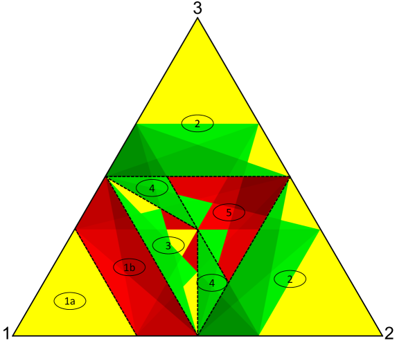
Figure 1: Borda vs. plurality for $m=3$. Regions colored green (yellow/red) indicate that Borda influence is greater than (equal to/smaller than) plurality influence

6.2 Further Comparisons

Analogous pairwise influence comparisons are depicted in the Appendix for all possible weight distributions $\mathbf{w}$ and $r\in\{r^{B},r^{C},r^{P},r^{PR},r^{S}\}$. Again, Borda’s high responsiveness to weight differences makes for more detailed case distinctions (see Figures A-1–A-4). By contrast, when plurality rule is compared to either Copeland, plurality runoff, or Schulze rule (Figure A-5), the recommendation always is simple and intuitive: plurality rule maximizes influence if you have the most votes. If anyone else has more votes, your influence is greater (at least weakly) under the respective other rule.

Recommendations to an influence-maximizing player are similar for Copeland vs. Schulze rule (Figure A-6): if you wield a plurality of votes, Schulze comes with greater influence; in case someone else has more votes, it is the opposite. For Copeland vs. plurality runoff (Figure A-7), the former gives greater influence to you if you have at least the second-most votes. If player 1 is to choose between plurality runoff and Schulze rule (Figure A-8), Schulze rule gives greater influence if $w_{1}$ is either largest or smallest; otherwise it is better to adopt plurality runoff.

6.3 Influence-maximizing Voting Rules

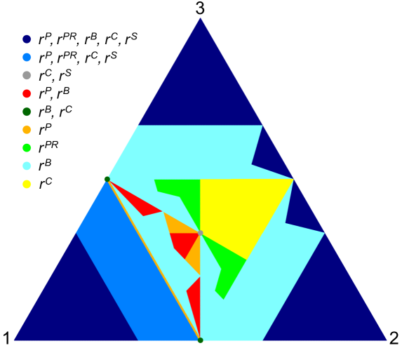
Figure 2: Maximal influence map for Borda, Copeland, plurality, plurality runoff, and Schulze rules for $m=3$.

Complementing pairwise comparisons as in Figures 1 and A-1–A-8, one can also check directly which of the considered voting rules maximizes a specific player’s a priori voting power at any given weight distribution. This is done in Figure 2: configurations of same color indicate the same set of influence-maximizing voting rules for player 1. (When the respective weight regions are lines or single points, we have manually enlarged them.) Tongue-in-cheek, Figure 2 provides a ‘map’ for influence-maximizing chairpersons – or for whoever has a say on the adopted voting rule and cares about a priori influence on decisions between three candidates. It also gives players 2 or 3 reason for criticizing adoption of a particular rule as biased.

7 Concluding Remarks

We have investigated how the distribution of voting power in a committee depends not only on voting weights but which of the many possible aggregation procedures for $m>2$ alternatives is adopted – from simple plurality voting to the elaborate computation of Schulze winners. Traditional measures of voting power, such as the Penrose-Banzhaf or Shapley-Shubik indices, fail to capture this. They should be accompanied by power indices for three or more alternatives.

One such index has been proposed and illustrated here. It evaluates how sensitive the collective choice under the given aggregation rule and weights is to preference changes by an individual player. The index is proportional to the probability for a random individual preference perturbation to affect the outcome, assuming preferences are independently uniformly distributed a priori. A dictator player’s voting power is normalized to one; a null player’s power is zero. The extent to which the distribution of weights matters differs across rules. So do comparative statics regarding the number of alternatives. How the adopted rule affects the distribution of voting power has been illustrated for (non-consensual) election of the IMF’s Managing Director by its Executive Board. Similar analysis might be conducted for multi-candidate election primaries, party conventions, corporate boards, etc.

Several case studies have shown with the benefit of hindsight how choice of a particular voting method may have affected big political decisions (cf., e.g., Leininger:1993; Tabarrok/Spector:1999; or Maskin/Sen:2016). We deem it worthwhile to evaluate collective choice methods also from an a priori perspective and ‘on average’. For the simplest case with three options, we have considered the power implications of all conceivable weight distributions among three players and identified differences in how several prominent rules translate weights into voting power. Except for Borda rule, precise knowledge about the distribution of voting weights is typically not needed for gaging the sensitivity of outcomes to preferences of a large, middle, or small player respectively. It is of course desirable to obtain results also for bigger numbers of players and alternatives in the future.

Our analysis hopefully encourages the extension of voting power analysis to richer choice settings. There is a great variety of single-winner rules that could be added to the influence map in Figure 2 (see, e.g., Aleskerov/Kurbanov:1999; [Ch. 7]Nurmi:2006; or Laslier:2012). And nothing in principle would preclude similar analysis for multi-winner elections (see, e.g., Elkind/Faliszewski/Skowron/Slinko:2017) or strategic voting equilibria, at least for restricted preference domains. It also seems worthwhile to investigate weight apportionment for two-tiered voting systems, such as US presidential elections, with more than two promising candidates. It is unknown, for instance, how the Penrose square root rule for the independent binary case (see, e.g, [Ch. 3.4]Felsenthal/Machover:1998) or Shapley linear rule for affiliated spatial preferences (cf. Kurz/Maaser/Napel:2018) extend to two-tiered plurality decisions or plurality voting with a runoff.

Appendix: Comparisons of voting rules for m$\,\mathbf{=3}$

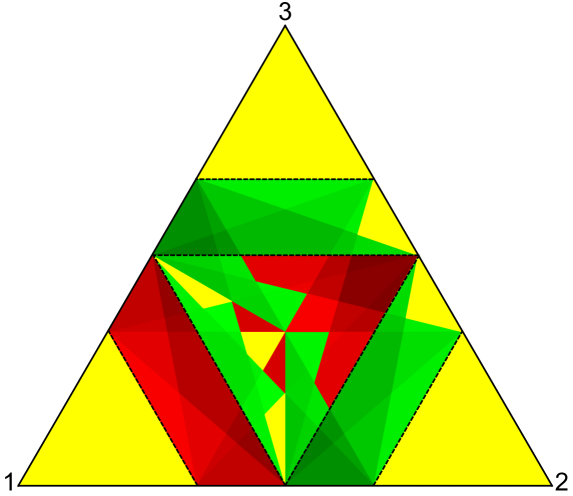
Figure A-1: Borda vs. plurality (repeated from p. 1)

Figure A-2: Borda vs. Copeland

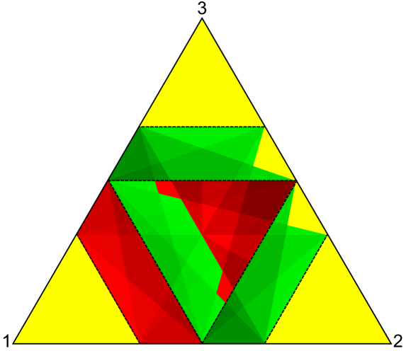
Figure A-3: Borda vs. plurality runoff

Figure A-4: Borda vs. Schulze

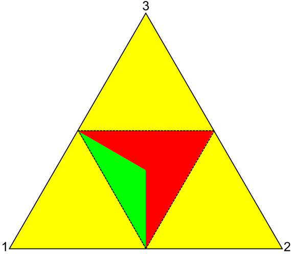
Figure A-5: Plurality vs. plurality runoff, Copeland and Schulze

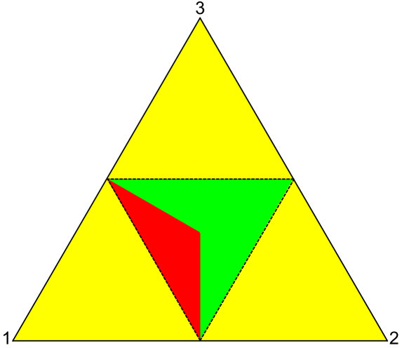
Figure A-6: Copeland vs. Schulze

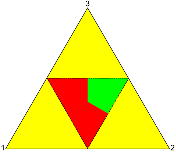
Figure A-7: Copeland vs. plurality runoff

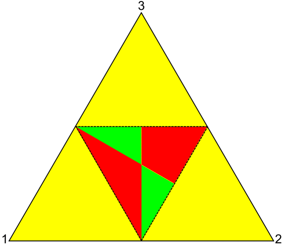
Figure A-8: Plurality runoff vs. Schulze

References

- [\citeauthoryearAleskerov, Kalyagin, and PogorelskiyAleskerov et al.2008] Aleskerov, F., V. Kalyagin, and K. Pogorelskiy (2008). Actual voting power of the IMF members based on their political-economic integration. Mathematical and Computer Modelling 48(9–10), 1554–1569.
- [\citeauthoryearAleskerov and KurbanovAleskerov and Kurbanov1999] Aleskerov, F. and E. Kurbanov (1999). Degree of manipulability of social choice procedures. In A. Alkan, C. D. Aliprantis, and N. C. Yannelis (Eds.), Current Trends in Economics, pp. 13–27. Berlin: Springer.
- [\citeauthoryearAmer, Carreras, and MagãnaAmer et al.1998] Amer, R., F. Carreras, and A. Magãna (1998). Extension of values to games with multiple alternatives. Annals of Operations Research 84(0), 63–78.
- [\citeauthoryearBanzhafBanzhaf1965] Banzhaf, J. F. (1965). Weighted voting doesn’t work: a mathematical analysis. Rutgers Law Review 19(2), 317–343.
- [\citeauthoryearBolgerBolger1986] Bolger, E. M. (1986). Power indices for multicandidate voting games. International Journal of Game Theory 15(3), 175–186.
- [\citeauthoryearBramsBrams1978] Brams, S. J. (1978). The Presidential Election Game. New Haven, CT: Yale University Press.
- [\citeauthoryearChua, Ueng, and HuangChua et al.2002] Chua, V. C. H., C. H. Ueng, and H. C. Huang (2002). A method for evaluating the behavior of power indices in weighted plurality games. Social Choice and Welfare 19(3), 665–680.
- [\citeauthoryearDubey and ShapleyDubey and Shapley1979] Dubey, P. and L. Shapley (1979). Mathematical properties of the Banzhaf power index. Mathematics of Operations Research 4(2), 99–131.
- [\citeauthoryearElkind, Faliszewski, Skowron, and SlinkoElkind et al.2017] Elkind, E., P. Faliszewski, P. Skowron, and A. Slinko (2017). Properties of multiwinner voting rules. Social Choice and Welfare 48(3), 599–632.
- [\citeauthoryearFelsenthal and MachoverFelsenthal and Machover1997] Felsenthal, D. S. and M. Machover (1997). Ternary voting games. International Journal of Game Theory 26(3), 335–351.
- [\citeauthoryearFelsenthal and MachoverFelsenthal and Machover1998] Felsenthal, D. S. and M. Machover (1998). The Measurement of Voting Power. Cheltenham, UK: Edward Elgar.
- [\citeauthoryearFreixasFreixas2005a] Freixas, J. (2005a). Banzhaf measures for games with several levels of approval in the input and output. Annals of Operations Research 137(1), 45–66.
- [\citeauthoryearFreixasFreixas2005b] Freixas, J. (2005b). The Shapley-Shubik index for games with several levels of approval in the input and output. Decision Support Systems 39(2), 185–195.
- [\citeauthoryearFreixas and ZwickerFreixas and Zwicker2003] Freixas, J. and W. S. Zwicker (2003). Weighted voting, abstention, and multiple levels of approval. Social Choice and Welfare 21(3), 399–431.
- [\citeauthoryearFreixas and ZwickerFreixas and Zwicker2009] Freixas, J. and W. S. Zwicker (2009). Anonymous yes-no voting with abstention and multiple levels of approval. Games and Economic Behavior 67(2), 428–444.
- [\citeauthoryearGarrett and TsebelisGarrett and Tsebelis1999] Garrett, G. and G. Tsebelis (1999). Why resist the temptation to apply power indices to the European Union? Journal of Theoretical Politics 11(3), 291–308.
- [\citeauthoryearGarrett and TsebelisGarrett and Tsebelis2001] Garrett, G. and G. Tsebelis (2001). Even more reasons to resist the temptation of power indices in the EU. Journal of Theoretical Politics 13(1), 99–105.
- [\citeauthoryearGibbardGibbard1973] Gibbard, A. (1973). Manipulation of voting schemes: a general result. Econometrica 41(4), 587–601.
- [\citeauthoryearHoller and NurmiHoller and Nurmi2013] Holler, M. J. and H. Nurmi (Eds.) (2013). Power, Voting, and Voting Power: 30 Years After. Heidelberg: Springer.
- [\citeauthoryearHsiao and RaghavanHsiao and Raghavan1993] Hsiao, C.-R. and T. E. S. Raghavan (1993). Shapley value for multichoice cooperative games, I. Games and Economic Behavior 5(2), 240–256.
- [\citeauthoryearKellyKelly1993] Kelly, J. S. (1993). Almost all social choice rules are highly manipulable, but a few aren’t. Social Choice and Welfare 10(2), 161–175.
- [\citeauthoryearKurz, Maaser, and NapelKurz et al.2018] Kurz, S., N. Maaser, and S. Napel (2018). Fair representation and a linear Shapley rule. Games and Economic Behavior 108, 152–161.
- [\citeauthoryearKurz, Mayer, and NapelKurz et al.2019] Kurz, S., A. Mayer, and S. Napel (2019). Weighted committee games. European Journal of Operational Research, doi: 10.1016/j.ejor.2019.10.023.
- [\citeauthoryearLaruelle and ValencianoLaruelle and Valenciano2001] Laruelle, A. and F. Valenciano (2001). Shapley-Shubik and Banzhaf indices revisited. Mathematics of Operations Research 26(1), 89–104.
- [\citeauthoryearLaruelle and ValencianoLaruelle and Valenciano2008] Laruelle, A. and F. Valenciano (2008). Voting and Collective Decision-Making. Cambridge: Cambridge University Press.
- [\citeauthoryearLaruelle and ValencianoLaruelle and Valenciano2012] Laruelle, A. and F. Valenciano (2012). Quaternary dichotomous voting rules. Social Choice and Welfare 38(3), 431–454.
- [\citeauthoryearLaslierLaslier2012] Laslier, J.-F. (2012). And the loser is …plurality voting. In D. S. Felsenthal and M. Machover (Eds.), Electoral Systems: Paradoxes, Assumptions, and Procedures, pp. 327–351. Berlin: Springer.
- [\citeauthoryearLeechLeech2002] Leech, D. (2002). Voting power in the governance of the International Monetary Fund. Annals of Operations Research 109(1–4), 375–397.
- [\citeauthoryearLeechLeech2003] Leech, D. (2003). Computing power indices for large voting games. Management Science 49(6), 831–837.
- [\citeauthoryearLeech and LeechLeech and Leech2013] Leech, D. and R. Leech (2013). A new analysis of a priori voting power in the IMF: Recent quota reforms give little cause for celebration. In M. J. Holler and H. Nurmi (Eds.), Power, Voting, and Voting Power: 30 Years After, pp. 389–410. Heidelberg: Springer.
- [\citeauthoryearLeiningerLeininger1993] Leininger, W. (1993). The fatal vote: Berlin versus Bonn. Finanzarchiv 50(1), 1–20.
- [\citeauthoryearMann and ShapleyMann and Shapley1962] Mann, I. and L. S. Shapley (1962). Values of large games, VI: evaluating the Electoral College exactly. Memorandum RM-3158-PR, The Rand Corporation.
- [\citeauthoryearMaskin and SenMaskin and Sen2016] Maskin, E. and A. Sen (2016). How majority rule might have stopped Donald Trump. New York Times. April 28, 2016.
- [\citeauthoryearMoulinMoulin1981] Moulin, H. (1981). The proportional veto principle. Review of Economic Studies 48(3), 407–416.
- [\citeauthoryearNapelNapel2019] Napel, S. (2019). Voting power. In R. Congleton, B. Grofman, and S. Voigt (Eds.), Oxford Handbook of Public Choice, Volume 1, Chapter 6, pp. 103–126. Oxford: Oxford University Press.
- [\citeauthoryearNapel and WidgrénNapel and Widgrén2004] Napel, S. and M. Widgrén (2004). Power measurement as sensitivity analysis: a unified approach. Journal of Theoretical Politics 16(4), 517–538.
- [\citeauthoryearNitzanNitzan1985] Nitzan, S. (1985). The vulnerability of point-voting schemes to preference variation and strategic manipulation. Public Choice 47(2), 349–370.
- [\citeauthoryearNurmiNurmi2006] Nurmi, H. (2006). Models of Political Economy. London: Routledge.
- [\citeauthoryearOwenOwen1975] Owen, G. (1975). Evaluation of a presidential election game. American Political Science Review 69(3), 947–953.
- [\citeauthoryearParkerParker2012] Parker, C. (2012). The influence relation for ternary voting games. Games and Economic Behavior 75(2), 867–881.
- [\citeauthoryearPelegPeleg1984] Peleg, B. (1984). Game Theoretic Analysis of Voting in Committees. Cambridge: Cambridge University Press.
- [\citeauthoryearPenrosePenrose1946] Penrose, L. S. (1946). The elementary statistics of majority voting. Journal of the Royal Statistical Society 109(1), 53–57.
- [\citeauthoryearRegenwetter, Grofman, Marley, and TsetlinRegenwetter et al.2012] Regenwetter, M., B. Grofman, A. A. J. Marley, and I. M. Tsetlin (2012). Behavioral Social Choice (2nd edition ed.). New York, NY: Cambridge University Press.
- [\citeauthoryearRiker and ShapleyRiker and Shapley1968] Riker, W. H. and L. S. Shapley (1968). Weighted voting: a mathematical analysis for instrumental judgements. In J. R. Pennock and J. W. Chapman (Eds.), Representation: Nomos X, Yearbook of the American Society for Political and Legal Philosophy, pp. 199–216. New York, NY: Atherton Press.
- [\citeauthoryearSatterthwaiteSatterthwaite1975] Satterthwaite, M. A. (1975). Strategy-proofness and Arrow’s conditions: existence and correspondence theorems for voting procedures and social welfare function. Journal of Economic Theory 10(2), 187–217.
- [\citeauthoryearSchulzeSchulze2011] Schulze, M. (2011). A new monotonic, clone-independent, reversal symmetric, and condorcet-consistent single-winner election method. Social Choice and Welfare 36(2), 267–303.
- [\citeauthoryearShapley and ShubikShapley and Shubik1954] Shapley, L. S. and M. Shubik (1954). A method for evaluating the distribution of power in a committee system. American Political Science Review 48(3), 787–792.
- [\citeauthoryearSmithSmith1999] Smith, D. A. (1999). Manipulability measures of common social choice functions. Social Choice and Welfare 16(4), 639–661.
- [\citeauthoryearTabarrok and SpectorTabarrok and Spector1999] Tabarrok, A. and L. Spector (1999). Would the Borda Count have avoided the civil war? Journal of Theoretical Politics 11(2), 261–288.
- [\citeauthoryearTchantcho, Lambo, Pongou, and EngoulouTchantcho et al.2008] Tchantcho, B., L. D. Lambo, R. Pongou, and B. M. Engoulou (2008). Voters’ power in voting games with abstention: influence relation and ordinal equivalence of power theories. Games and Economic Behavior 64(1), 335–350.
- [\citeauthoryearVon Neumann and MorgensternVon Neumann and Morgenstern1953] Von Neumann, J. and O. Morgenstern (1953). Theory of Games and Economic Behavior (3rd ed.). Princeton, NJ: Princeton University Press.