Ground-state properties of the one-dimensional Hubbard model with pairing potential

Abstract

We consider a modification of the one-dimensional Hubbard model by including an external pairing potential. Guided by analytic bosonization results, we quantitatively determine the grand-canonical zero-temperature phase diagram using both finite and infinite density matrix renormalization group algorithm based on the formalism of matrix product states and matrix product operator, respectively. By computing various local quantities as well as the half-system entanglement, we are able to distinguish between Mott, metallic and superconducting phases. We point out the compressible nature of the Mott phase and the fully gapped nature of the many-body spectrum of the superconducting phase, in the presence of explicit U(1)-charge symmetry breaking.

1 Introduction

Long-range quantum correlations often fully characterize the nature of a quantum phase in many-particle systems. An abrupt change of correlations typically occurs at quantum phase transitions [1]. As a quantitative measure of quantum correlations, the entanglement entropy plays a central role, potentially able to signal quantum phase transitions or to characterize critical gapless phases [2].

To define the entanglement entropy [3], one bipartites the quantum system into two parts $A$ and $B$. One then introduces a density matrix $\rho=|\Psi\rangle\langle\Psi|$ of a pure quantum state $|\Psi\rangle$, and obtains the reduced density matrix $\rho_{A}=\mbox{Tr}_{B}\rho$ by tracing out the subsystem $B$. The entanglement entropy is the von Neumann entropy, which is given by $S_{A}=-\mbox{Tr}(\rho_{A}\ln\rho_{A})$. Since we will consider zero-temperature properties in the following, we will compute entanglement properties using the ground-state as wavefunction $|\Psi\rangle$.

In order to find the ground state in quantum many-particle systems, the density matrix renormalization group [4] (DMRG) method is suitable, especially in one dimension. The connection between DMRG and tensor networks was first recognized by the quantum information community [5]. A detailed reformulation of DMRG in terms of matrix product states (MPS) was reviewed by Schollwöck [6]. The generalization of MPS to handle two-dimensional systems was carried out, and the projected entangled pair state (PEPS) was introduced [7]. For critical systems, the multi-scale entanglement renormalization ansatz (MERA) is useful [8]. When a Hamiltonian has translational invariance, we can use the so-called infinite DMRG (iDMRG) [9], in which we assume that the matrices in the MPS are identical. Without entering into too much details, let us simply mention that we update a few matrices and environments to converge to the ground-state $|\Psi_{0}\rangle$ with the iDMRG method.

One motivation of introducing a pairing term is to model condensed matter quasi-1D electronic quantum wires weakly coupled to a thin (3D) supercconductor sheet. Such a set-up has been proposed by Kitaev [10] to realize boundary Majorana fermions by proximity effect with a p-wave superconductor. Our proposal involves a singlet (s-wave or d-wave) superconductor that could be realized using e.g. a (quasi-2D) high-Tc superconductor.

Also, since atoms with an odd number of neutrons [11] are fermions and thus obey the same statistical rules as electrons, some cold atoms [12] in an optical lattice can mimic the behaviors of electrons in a real solid material. In cold atom experiments, quantum gas microscope [13] was used to create and image an antiferromagnet, a phase in which one atom occupies each lattice site, and the spins of neighboring atoms point in opposite directions [14]. This provides us with a motivation to consider the singlet state of neighboring atoms with the pairing interaction.

Since experimentalists can design ultracold many-fermion systems loaded on quasi one-dimensional optical lattices [15], the one-dimensional fermion Hubbard model has become a physical reality. Quite interestingly, the attractive Hubbard model which is the simplest model to describe pairing and superconductivity in a fermionic system can also be realized [16]. In our case, the repulsive Hubbard model with an additional pairing potential, providing a tendency to form nearest-neighbor singlet pairs, could also be realized in fermionic systems, for instance by proximity effect with a singlet superconductor.

The purpose of this paper is to compute the ground-state phase diagram of the one-dimensional Hubbard model with a (singlet) pairing potential. To do so, guided by analytic bosonization results, we apply two standard numerical algorithms (finite and infinite DMRG) separately to optimize the matrices in the MPS. The results obtained by both methods are consistent with each other. By changing the chemical potential, a quantum phase transition occurs between gapless and gapped phases, as can be measured from the scaling of the entanglement entropy.

2 Model and analytical treatments

2.1 Model and some exact transformations

We consider a simple generalization of the Hubbard model on a one-dimensional (1D) lattice :

$$H = -t\sum_{\langle ij\rangle}(c^{\dagger}_{i\uparrow}c_{j\uparrow}+c^{\dagger}_{j\uparrow}c_{i\uparrow}+c^{\dagger}_{i\downarrow}c_{j\downarrow}+c^{\dagger}_{j\downarrow}c_{i\downarrow})$$ (1)

$$+U\sum_{i}(n_{i\uparrow}-\frac{1}{2})(n_{i\downarrow}-\frac{1}{2})-\mu\sum_{i}(n_{i\uparrow}+n_{i\downarrow})$$

$$-\Delta\sum_{\langle ij\rangle}(c^{\dagger}_{i\uparrow}c^{\dagger}_{j\downarrow}+c^{\dagger}_{j\uparrow}c^{\dagger}_{i\downarrow}+c_{i\downarrow}c_{j\uparrow}+c_{j\downarrow}c_{i\uparrow}),$$

where $c$ and $c^{\dagger}$ are the usual spin-1/2 fermion annihilation and creation operators, $n_{i\sigma}=c^{\dagger}_{i\sigma}c_{i\sigma}$ is the local spin-resolved density and $\langle ij\rangle$ stands for nearest neighboring sites on the 1D chain. We fix the hopping strength $t=1$ (as unit of energy) and vary the other three parameters: the on-site Coulomb repulsion $U$, the chemical potential $\mu$, and the pairing strength $\Delta$. The role of the chemical potential is to control the average number of fermions in the system. Note that the (bond) singlet pairing potential does not conserve the particle number so that the model only has SU(2) spin symmetry. Physically, such a potential may account for the proximity effect of a nearby singlet superconductor. Without pairing potential, i.e. for $\Delta=0$, we recover the standard one-dimensional (repulsive) Hubbard model which will be used for benchmark calculations as it is exactly solvable [17, 18].

Let us make some additional remarks about the symmetries of this model. Half-filling will correspond to $\mu=0$ obviously and the phase diagram will be symmetric under $\mu\leftrightarrow-\mu$. Moreover, when $\mu=0$, applying a particle-hole symmetry only on odd sites ($d_{2i,\sigma}=c_{2i,\sigma}$ and $d_{2i+1,\sigma}=c^{\dagger}_{2i+1,-\sigma}$) amounts to exchanging the hamiltonian parameters as $(t,U,\mu=0,\Delta)\leftrightarrow(\Delta,U,\mu=0,t)$, i.e. exchanging the role of $t$ and $\Delta$.

In the non-interacting case ($U=0$), the model is quadratic so that it can be diagonalized in Fourier space using a Bogoliubov transformation to get

$$H_{0}=\sum_{k}E_{k}(\alpha^{\dagger}_{k}\alpha_{k}+\beta^{\dagger}_{k}\beta_{k})$$ (2)

with a dispersion $E_{k}=\pm\sqrt{(\varepsilon_{k}-\mu)^{2}+(\Delta\cos k)^{2}}$ where $\varepsilon_{k}=-2t\cos k$ is the tight-binding dispersion. In particular, for a generic filling (i.e. a generic $\mu$ value), we have a one-dimensional superconductor with a finite gap . Indeed, there is no U(1) symmetry breaking in this model (since the particle number conservation is explicitly broken) and, hence, no emergent zero-energy Goldstone modes. On general grounds, we expect that this superconducting phase will persists in some range of the phase diagram, even in the presence of a finite repulsive $U$. Note also that, in this gapped superconducting phase, the compressibility is finite though.

We now transform the Hamiltonian in a convenient form. Using the Bogoliubov rotation

$$c_{j\uparrow}=\cos\frac{\theta}{2}f_{j\uparrow}-\sin\frac{\theta}{2}f^{\dagger}_{j\downarrow},$$

$$c^{\dagger}_{j\downarrow}=\sin\frac{\theta}{2}f_{j\uparrow}+\cos\frac{\theta}{2}f^{\dagger}_{j\downarrow},$$ (3)

where $t+i\Delta=\sqrt{t^{2}+\Delta^{2}}e^{-i\theta}$ we can rewrite Eq. (1) in the form

$$H = -\sqrt{t^{2}+\Delta^{2}}\,\sum_{j,\sigma}(f^{\dagger}_{j+1\sigma}f_{j\sigma}+f^{\dagger}_{j\sigma}f_{j+1\sigma})$$ (4)

$$+U\sum_{j}\left(f^{\dagger}_{j\uparrow}f_{j\uparrow}-\frac{1}{2}\right)\left(f^{\dagger}_{j\downarrow}f_{j\downarrow}-\frac{1}{2}\right)$$

$$-\frac{\mu t}{\sqrt{t^{2}+\Delta^{2}}}\sum_{j}(f^{\dagger}_{j\uparrow}f_{j\uparrow}+f^{\dagger}_{j\downarrow}f_{j\downarrow})$$

$$-\frac{\mu\Delta}{\sqrt{t^{2}+\Delta^{2}}}\sum_{j}(f^{\dagger}_{j\uparrow}f^{\dagger}_{j\downarrow}+f_{j\downarrow}f_{j\uparrow}),$$

showing that $\mu$ is giving both a chemical potential and an s-wave pairing interaction for the $f$ fermions. Eq. (4) is $\mathrm{SU(2)}$ symmetric, and since the Bogoliubov rotation, Eq. (2.1), leaves the expression of the spin operators in fermions invariant, this rules out all non-$\mathrm{SU(2)}$ singlet ground states for the Hamiltonian of Eq. (1) such as spin-density wave or triplet superconductivity.

2.2 Half-filling

Let us first consider the half-filled case. For $\mu=0$, the Hamiltonian (4) reduces to:

$$H = -\sqrt{t^{2}+\Delta^{2}}\,\sum_{j,r=\pm}(f^{\dagger}_{j+1r}f_{jr}+f^{\dagger}_{jr}f_{j+1r})$$ (5)

$$+U\sum_{j}\left(n_{j+}-\frac{1}{2}\right)\left(n_{j-}-\frac{1}{2}\right).$$

For $U>0$ the Hamiltonian (5) has a charge gap and a $c=1$ gapless spin mode (Mott insulator), while for $U<0$ it has gapped spin modes and a $c=1$ gapless charge mode (Luther-Emery liquid). Since $n_{j\uparrow}-n_{j\downarrow}=n_{j+}-n_{j-}$ and $c^{\dagger}_{j\uparrow}c_{j\downarrow}=f^{\dagger}_{j+}f_{j-}$, the spin density wave correlations of the original $c$ fermions are the same as the ones of the $f$ fermions. However, if we turn to the density, since

$$n_{j\uparrow}+n_{j\downarrow}-1=\cos\theta(n_{j+}+n_{j-}-1)-\sin\theta(f^{\dagger}_{j+}f^{\dagger}_{j-}+f_{j-}f_{j+}),$$ (6)

the density-density correlations of the $c$ fermions are a weighted sum of those of the $f$ fermions and the s-wave superfluid correlations of the same $f$ fermions. In the Mott insulating state, both of those correlations are decaying exponentially, so the density-density correlations show an exponential decay. In the Luther-Emery liquid, the density-density correlations of the $c$ fermions decay as a power law with distance. However, the superfluid component contributes $\sin^{2}\theta/j^{1/K_{c}}$ to the density-density correlations, where $K_{c}$ is the charge Luttinger exponent. Since in the Hubbard model with attractive interaction, $K_{c}>1$, this contribution dominates the $\cos^{2}\theta/j^{2}$ term coming from the density-density correlations.

To summarize, at half-filling the ground state is always a phase with $c=1$: A Mott insulator when $U>0$, a Luther-Emery liquid when $U<0$. But, the Bogoliubov rotation (2.1), turns the density-density correlations and the s-wave superfluid correlation functions into weighted sums of the same correlation functions in the standard 1D Hubbard model. Now, we turn to bosonization [19] to consider the effect of the chemical potential $\mu$.

2.3 Bosonization approach

With $\mu\neq 0$, we need to consider Eq. (4). The third term of Eq. (4) is a chemical potential for the $f$ fermions, while the last term is an s-wave pairing. To make further progress, it is necessary to use the bosonized representation [19] of the Hamitonian (4). We find

$$H = H_{c}+H_{s}+H_{cs},$$ (7)

$$H_{c} = \int\frac{dx}{2\pi}\left[u_{c}K_{c}(\pi\Pi_{c})^{2}+\frac{u_{c}}{K_{c}}(\partial_{x}\phi_{c})^{2}\right]+\frac{\sqrt{2}h}{\pi}\int dx\partial_{x}\phi_{c}$$ (8)

$$-\frac{2g_{3}}{(2\pi\alpha)^{2}}\int dx\cos\sqrt{8}\phi_{c},$$

$$H_{s} = \int\frac{dx}{2\pi}\left[u_{s}K_{s}(\pi\Pi_{s})^{2}+\frac{u_{s}}{K_{s}}(\partial_{x}\phi_{s})^{2}\right]+\frac{2g_{1\perp}}{(2\pi\alpha)^{2}}\int dx\cos\sqrt{8}\phi_{s},$$ (9)

$$H_{cs} = -\frac{2\Omega}{\pi\alpha}\int dx\cos\sqrt{2}\theta_{c}\cos\sqrt{2}\phi_{s},$$ (10)

where $[\phi_{\nu}(x),\Pi_{\nu^{\prime}}(x^{\prime})]=i\delta(x-x^{\prime})\delta_{\nu,\nu^{\prime}}$ and $\pi\Pi_{\nu}=\partial_{x}\theta_{\nu}$, with $\nu=c$ for charge excitations and $\nu=s$ for spin excitations. The short distance cutoff, of the order of the lattice spacing is $\alpha$, and the parameters in the bosonized Hamiltonian are given by

$$u_{c}K_{c}=u_{s}K_{s}=v_{F},$$

$$\frac{u_{c}}{K_{c}}=v_{F}+\frac{U\alpha}{\pi},$$

$$\frac{u_{s}}{K_{s}}=v_{F}-\frac{U\alpha}{\pi},$$

$$g_{3}=g_{1\perp}=U\alpha,$$

$$h=\frac{\mu t}{\sqrt{t^{2}+\Delta^{2}}},$$

$$\Omega=\frac{\mu\Delta}{\sqrt{t^{2}+\Delta^{2}}},$$ (11)

with $v_{F}=2\sqrt{t^{2}+\Delta^{2}}\alpha$. The simplest case is $U<0$. The spin Hamiltonian $H_{s}$ is gapped with $\langle\phi_{s}\rangle=0$, while the charge Hamiltonian $H_{c}$ remains gapless. Physically, the fermions are already paired, but there is only quasi-long range superconducting order. With $\Omega\neq 0$, the pairing term $\sim e^{i\sqrt{2}\theta_{c}}$ simply provides the necessary symmetry breaking and gives rise to a long range superconducting order with $c=0$.

The case of $U>0$ is more complicated. The Hamiltonian $H_{c}$ is gapped, with $\langle\phi_{c}\rangle=0$, while $H_{s}$ is gapless. However, the term proportional to $\Omega$ gives rise to a fully gapped ground state with $\langle\theta_{c}\rangle=0$ and $\langle\phi_{s}\rangle=0$. Since the dual fields $\theta_{c}$ and $\phi_{c}$ cannot be ordered simultaneously, the $g_{3}$ and $\Omega$ term are competing with each other and a phase transition is expected. There are two different scenarios for the transition depending on the ratio $\Delta/t$. First, in the absence of the chemical potential, the transition is driven by $\Omega$. A weak chemical potential term ($t\ll\Delta$), simply drives the charge doping in the superconducting phase. A more detailed picture of that scenario is discussed in the Appendix. Second, in the absence of charge-spin coupling (10), the $h$ term would give rise to a commensurate-incommensurate transition [19, 20, 21] closing the charge gap, yielding a two-component Tomonaga-Luttinger liquid having two $c=1$ modes for spin and charge of different velocities. At the transition point [19], we would have $K_{c}=1/2$ with $K_{s}=1$ because of $\mathrm{SU(2)}$ spin symmetry. Now, Eq. (10), implies that the scaling dimension of $\Omega$ at the transition point is $2-1/(2K_{c})-K_{s}/2=1/2$, so that for $0<|\Delta|\ll t$, a gap $M\sim\frac{v_{F}}{\alpha}\left(\frac{\Omega\alpha}{v_{F}}\right)^{2}$ immediately opens both in the spin and the charge modes. The superconducting state with $\langle\theta_{c}\rangle=0$ and $\langle\phi_{s}\rangle=0$ is then formed.

These two scenarios can be distinguished by considering the evolution of the charge density with $\mu$. In both cases, there is according to Eq. (6) a contribution proportional to $\langle\cos\sqrt{2}\theta_{c}\cos\sqrt{2}\phi_{s}\rangle$. That contribution is non-singular since the charge modes are always gapped, and can be obtained from linear response. However, in the vicinity of the commensurate-incommensurate transition [20, 21], the particle density $\langle n_{+}+n_{-}-1\rangle\sim(h-h_{c})^{1/2}$ giving rise to a kink in the density at the transition between the Mott insulator and the superfluid. Summing the two contributions, the fermion density varies as

$$\langle n_{j\uparrow}+n_{j\downarrow}-1\rangle=A(\Delta,t,U)\mu+B(\Delta,t,U)\sqrt{\mu-\mu_{c}}\Theta(\mu-\mu_{c}),$$ (12)

when $\Delta\ll t$. By contrast, when $\Delta\gg t$, a large gap is present on both sides of the transition, and the density varies smoothly with the chemical potential.

$$\langle n_{j\uparrow}+n_{j\downarrow}-1\rangle=C(\Delta,t,U)\mu+D(\Delta,t,U)f(\mu),$$ (13)

In the Appendix, we show that at the transition, $f(\mu)\sim(\mu-\mu_{c})\ln|\mu-\mu_{c}|$, i.e. there is only a vertical tangent instead of a slope discontinuity.

2.4 Friedel oscillations

So far, we have considered an infinite chain. With a finite chain of $N$ sites, we have to introduce two fictitious sites $0$ and $N+1$ such that

$$c_{0\sigma}=c_{N+1\sigma}=0.$$ (14)

Using Eq. (2.1) this translates into $f_{0+}=f^{\dagger}_{0-}=0$ and $f_{N+1+}=f^{\dagger}_{N+1-}=0$. Thus, the $f$ fermions obey the same open boundary conditions as the original fermions. In bosonization, the boson fields [19, 23] in Eqs. (8)–(9) have to satisfy

$$\phi_{\nu}(0)=\phi_{\nu}(N+1)=0,$$ (15)

for $\nu=c,s$. In the MI phase, the conditions (15) are already satisfied in the bulk by the charge modes. As the edge does not perturb the ordering of the charge modes, only its effect the spin modes needs to be analyzed. In facts [24, 25, 26], the boundary conditions being $\mathrm{SU(2)}$ symmetric, only $\langle\cos\sqrt{2}\phi_{s}\rangle(j)\sim j^{-1/2}\neq 0$ (near the left edge). Taking into account the ordering of the charge modes, only the Bond Order Wave (BOW) order parameter $\langle\cos\sqrt{2}\phi_{c}\cos\sqrt{2}\phi_{s}\rangle\sim j^{-1/2}$ expectation value shows power law oscillations. This translates into

$$\langle\sum_{\sigma}(c^{\dagger}_{j+1\sigma}c_{j\sigma}+c^{\dagger}_{j\sigma}c_{j+1\sigma})\rangle\sim\frac{(-)^{j}}{\sqrt{\frac{N+1}{\pi}\sin\left(\frac{\pi j}{N+1}\right)}}.$$ (16)

In the SC phase, the conditions (15) are already satisfied in the bulk by the spin modes. For the charge modes, however, the boundary conditions (15) impose that the superconducting order parameter vanishes at the edge and make the BOW order parameter nonzero. Moving into the bulk, the BOW operator expectation value decays exponentially, while the SC order parameter recovers its bulk expectation value.

3 Numerical methods

3.1 MPO formalism

We shall now focus exclusively on the (more complicated) $U>0$ case and use both finite and infinite size DMRG. Since the Hamiltonian has translation symmetry, we construct the corresponding matrix product operator (MPO), which acts on matrix product state (MPS). By performing the usual matrix multiplication, we can check that the following MPO does represent our Hamiltonian:

$$\left(\begin{array}[]{cccccc}1&c^{\dagger}_{i\uparrow}&c^{\dagger}_{i\downarrow}&c_{i\uparrow}&c_{i\downarrow}&U(n_{i\uparrow}-\frac{1}{2})(n_{i\downarrow}-\frac{1}{2})-\mu(n_{i\uparrow}+n_{i\downarrow})\\ 0&0&0&0&0&-tc_{i\uparrow}-\Delta c^{\dagger}_{i\downarrow}\\ 0&0&0&0&0&-tc_{i\downarrow}+\Delta c^{\dagger}_{i\uparrow}\\ 0&0&0&0&0&tc^{\dagger}_{i\uparrow}+\Delta c_{i\downarrow}\\ 0&0&0&0&0&tc^{\dagger}_{i\downarrow}-\Delta c_{i\uparrow}\\ 0&0&0&0&0&1\end{array}\right)$$ (17)

where we omit the boundary operators. Obviously, we need to take care of ordering for fermions when we carry out iDMRG by acting with the MPO on the MPS.

Let us assume that the physical index $\sigma_{i}$ labels the state on the $i$-th site. For the Hubbard model, $\sigma_{i}=(\alpha_{i},\beta_{i})$, where $\alpha_{i}(\beta_{i})=0$ or $1$ means that there is a vacancy or occupation of the spin-up (down) fermion at the $i$-th site, respectively. The state of the Fock space for a $L$-lattice system is thus written in terms of the creation operators $c^{\dagger}_{i\uparrow}$ and $c^{\dagger}_{i\downarrow}$ as follows:

$$|\sigma_{0}\cdots\sigma_{L-1}\rangle=(c^{\dagger}_{0\uparrow})^{\alpha_{0}}(c^{\dagger}_{0\downarrow})^{\beta_{0}}\cdots(c^{\dagger}_{L-1\uparrow})^{\alpha_{L-1}}(c^{\dagger}_{L-1\downarrow})^{\beta_{L-1}}|0\rangle\,.$$ (18)

It is important to maintain the order of the fermions in the state of the Fock space to handle the minus sign caused by the exchange of fermion. We adopt the order of spin-up first and spin-down next as above.

For iDMRG with a two-site unit cell, two tensors, $A$ and $B$, in the MPS are repeated as $\cdots ABABAB\cdots$ with the usual matrix multiplication. The tensors, $A_{ab}^{\sigma}$ and $B_{cd}^{\rho}$, have three indices, among which the physical index $\sigma$ and $\rho$ takes a value from $0$ to $3$ for our model. For the degree of freedom of the internal bond, the indices $a$ (left) and $b$ (right) for $A$ range from $0$ to $\chi-1$, where $\chi$ is the dimension of the internal bond. The Schmidt coefficients between $A$ and $B$, and between $B$ and $A$, are denoted by $\lambda^{AB}$ and $\lambda^{BA}$, respectively. Thus, a state in the space of matrix product states is written as

$$|\Psi\rangle=\sum_{\cdots\sigma\rho\nu\eta\cdots}\mbox{Tr}(\cdots A^{\sigma}_{ab}\lambda^{AB}_{b}B^{\rho}_{bc}\lambda^{BA}_{c}A^{\nu}_{cd}\lambda^{AB}_{d}B^{\eta}_{de}\cdots)|\cdots\sigma\rho\nu\eta\cdots\rangle,$$ (19)

where Tr means that the indices of the internal bonds $a,b,c,d,\cdots$ are summed up. Scaling properties will be sought by increasing $\chi$

Regardless of the $t$, $U$, $\mu$, and $\Delta$ values used in our calculations, we have observed a smooth convergence. Our numerical DMRG results show that the ground-state solutions fall into two classes: MPS are either of the form $\cdots ABABAB\cdots$ (i.e. unit cell of two sites that we will identify as a Mott phase) near half filling ($\mu=0$), or uniform $\cdots AAAAAA\cdots$ further away from half-filling, that we will identify as metallic or superconducting phases, for $\Delta=0$ or non-zero, respectively.

3.2 Phase diagram

We will present data obtained using the infinite DMRG (with a two-site unit cell) as well as the finite-size algorithm for chain length up to $L=512$. After computing the ground state $|\Psi\rangle$, we compute local quantities such as the bond energy and the local densities and we also use the half-chain entanglement entropy to determine if the system is critical and, if so, what is its central charge.

By contraction of the Hamiltonian bond operator with the ground-state MPS, we obtain the bond energy. Close to half-filling, since the MPS has an ABAB form, we obtain alternating bond energies on even and odd bonds. We have observed however that the modulation seems to vanish for $\chi\rightarrow\infty$. To be more quantitative, we determine the half-chain entanglement entropy $S$, which is related to the Schmidt coefficients $\lambda_{a}$ as

$$S=-\sum^{\chi-1}_{a=0}\lambda^{2}_{a}\ln\lambda^{2}_{a}.$$ (20)

The Schmidt coefficients $\lambda_{a}$ are obtained when we perform a singular value decomposition (SVD) to find the matrices $A$ and $B$ in the MPS. Normalization of $\sum^{\chi-1}_{a=0}\lambda^{2}_{a}=1$ guarantees $\langle\Psi|\Psi\rangle=1$. For the $\cdots ABABAB\cdots$ solution, we obtain two different values of the entanglement entropy: $S_{o}$ with $\lambda^{AB}$ on the odd bonds and $S_{e}$ with $\lambda^{BA}$ on the even ones.

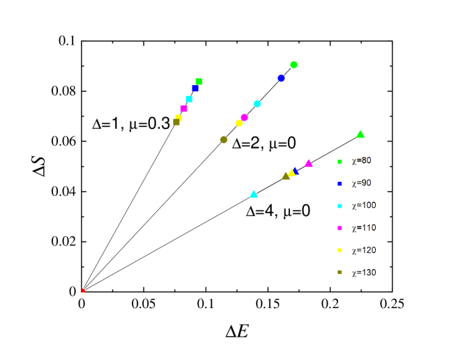
Figure 1: The entanglement entropy difference $\Delta S$ versus the bond energy difference $\Delta E$ for three cases by setting $t=1$ and $U=4$. The different colors of the data points are corresponding to the difference values of $\chi$. We note the particular order of the data points for the case of $\Delta=4$, $\mu=0$. The linear fits are compatible with a zero intercept, i.e. $\Delta S$ and $\Delta E$ are proportional.

The calculation shows that, close to half-filling, both the bond energy and the entanglement entropy have a finite modulation. In such a case, the energy difference $\Delta E=E_{e}-E_{o}$ and the entropy difference $\Delta S=S_{o}-S_{e}$ are proportional to each other [22]. In Fig. 1, we present the $\chi$-dependence of $\Delta E$ versus $\Delta S$. The numerical results confirm that $\Delta S$ is proportional to $\Delta E$ to a very high accuracy of $10^{-6}$. We conclude that $\Delta S=0$ and $\Delta E=0$ for the infinite bond dimension of $\chi=\infty$, as expected.

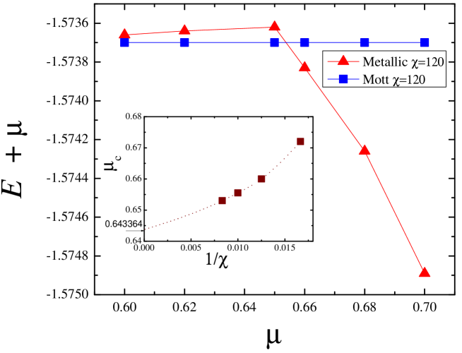
Figure 2: Ground state energy (shifted by $\mu$) versus $\mu$ showing a level crossing between the Mott-insulating and the metallic iDMRG solutions, at a finite $\chi$ value. We have set $t=1$, $U=4$ and $\Delta=0$. Inset: the scaling of the crossing points with $1/\chi$ agrees with the exact transition point at $\mu_{+}\simeq 0.643364$.

In order to determine the Mott transition, characterized by a change in the compressibility, we compute the (average) ground state energy $E=(E_{e}+E_{o})/2$ vs the chemical potential $\mu$ starting from $\mu=0$. On the other hand, we can also compute the ground-state energy in the uniform solution by decreasing $\mu$ (starting from large values). In each iDMRG calculation, the tensors of the initial environment are given by the previous solution of the different $\mu$. First, as a benchmark, we plot in Fig. 2 the evolution of the ground state energy for $\Delta=0$, where we find a level-crossing at a critical $\mu_{c}$. In full care of the entanglement, corresponding to $\chi\rightarrow\infty$, our extrapolation of $\mu_{c}$ is quite close to the exact value $\mu_{+}$ found using the Lieb-Wu method [17, 18] and it corresponds to the well-known second-order phase transition between an incompressible Mott phase and a metallic one.

We also compute the density, i.e. the expectation value of the occupation number $n=\langle n_{i,\uparrow}+n_{i,\downarrow}\rangle$, as a function of $\mu$ as shown in Fig. 3 for several values of the pairing strength $\Delta$ and $U=4$. For $\Delta=0$, we do observe an incompressible phase around $\mu=0$ and a transition point identical to the previous one, see Fig. 2. For $\Delta>0$, the compressibility (which is the slope of $n$ vs $\mu$) is always finite but we do observe a sudden change for some critical $\mu_{c}$, which we identify as the phase transition between Mott and superconducting phases. The finite compressibility is a consequence of Eq. (2.1). The fermion density is a weighted sum of the density of the Bogoliubov quasiparticles and of their superconducting order parameter. The latter responds linearly to $\mu$ according to Eq. (4) resulting in a nonzero compressibility even in the Mott phase.

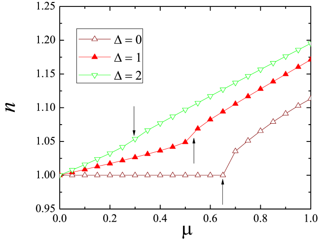
Figure 3: Density $n$ versus chemical potential $\mu$ for $U=4$, $t=1$ and $\chi=120$. For different values $\Delta$, we observe an abrupt change of the slope $\partial n/\partial\mu$.

As a concluding remark about this section, we have observed that the critical $\mu_{c}$ varies with the pairing strength $\Delta$ so that we can summarize the numerical results in the phase diagram shown in Fig. 4. On top of our numerical data, we provide a qualitative sketch of the full phase diagram but it is difficult numerically to determine what happens for large $\Delta$ at $\mu=0$. In this region, we can use the partial particle-hole transformation that was discussed in Sec. 2. Indeed, for $\mu=0$, the model with parameters $(t=1,U,\Delta)$ at large $\Delta$, which is difficult to analyze, is equivalent to the one at $(t=\Delta,U,\Delta=1)$ which is simply a tight-binding chain with small perturbation. In this case, we do expect a Mott phase with a very small gap [18], hence a very small Mott region.

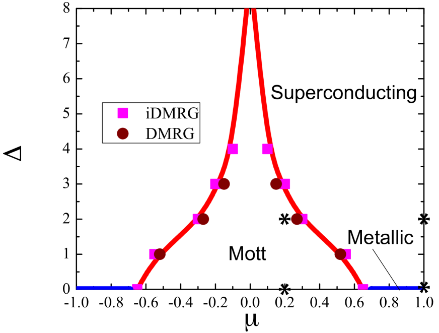
Figure 4: Numerical phase diagram of the one-dimensional Hubbard model at $t=1$ and $U=4$, as a function of the chemical potential $\mu$ and the singlet pairing potential $\Delta$, obtained from iDMRG (magenta squares) and DMRG (purple circles, $L=128$). The red line is a guide to the eyes. The region of the Mott-insulating phase shrinks for smaller $U$. Star symbols correspond to the points where local quantities are plotted in Fig. 5.

3.3 Local observables and exponents

In order to confirm that there is no breaking of the translation symmetry in the thermodynamic limit, we also plot in Fig. 5 several local quantities measured by finite-size DMRG (with open boundary conditions) in several points of the phase diagram. Panels (a-b) correspond to the pure Hubbard model respectively in the Mott and metallic phase. In the Mott phase, the density is locked to $n_{\uparrow}=n_{\downarrow}=n/2=0.5$ per site since the chemical potential is smaller than the gap and we do observe Friedel oscillations in the bond kinetic energy, similar to the well-known oscillations in Heisenberg spin chains [22], which can be fitted as $1/x^{0.55}$ in good agreement with the predicted $1/\sqrt{x}$ knowing that logarithmic corrections are present [19]. In the metallic phase for a generic filling, oscillations are incommensurate and can provide accurate information about Luttinger exponents etc [23, 27]. For finite $\Delta$ and small $|\mu|$, see Fig. 5c, this is the generalized Mott phase with very small density fluctuations (non-zero since there is a finite compressibility) and power-law Friedel oscillations both in the bond kinetic energy and in the bond pairing energy: we have attempted to fit the pairing modulations with a power-law from the edge, which leads to an exponent 0.71; however, fitting the modulation measured in the center of the chain as a function of $1/L$ leads to an exponent $0.51$ in perfect agreement with analytic prediction, see Eq. (16). Last, in the superconducting phase, see Fig. 5d, the Friedel oscillations in all local quantities are short-range and can be fitted with an exponential form, as expected for a fully gapped phase.

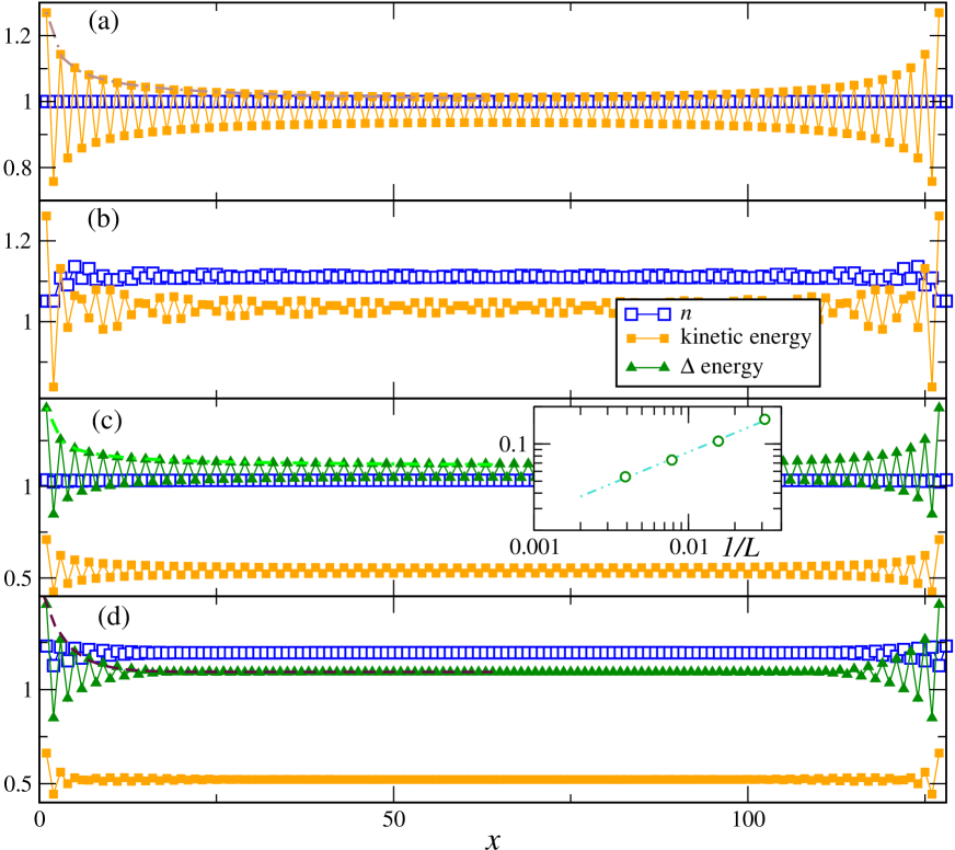
Figure 5: Local quantities of the one-dimensional Hubbard model at $t=1$ and $U=4$, obtained from DMRG on chains of length $L=128$ at various points in the phase diagram (star symbols in Fig. 4). From top to bottom, parameters $(\mu,\Delta)$ are: (a) (0.2,0) in the Mott phase of the pure Hubbard model; (b) (1,0) in the metallic phase of the pure Hubbard model; (c) (0.2,2) in the Mott phase of our model; (d) (1,2) in the superconducting phase. Inset of panel (c) shows the pairing modulation measured in the center of the chain as a function of $1/L$ in logarithmic scale, fitted with an exponent $1/L^{0.51}$.

Note that the physics of our model is rather different from the extended Hubbard model which is known to host long-range ordered BOW [28].

3.4 Entanglement entropy scaling

It is well-established that block entanglement entropy scaling can be used to determine if the ground-state is gapped or critical. In the later case, the central charge of the underlying Conformal Field Theory (CFT) can also be computed [29]. In Fig. 6, we present the half-chain entanglement entropy $S=(S_{o}+S_{e})/2$, which is obtained from iDMRG. In agreement with our local measurements from the previous section, we do observe a rather flat plateau region around $\mu=0$, at least for $\Delta$ not too large, corresponding to the Mott phase obtained from the compressibility data. Note that the size of the plateau is decreasing with $\Delta$ so that it is still difficult to determine the physics for large $\Delta$ at $\mu=0$.

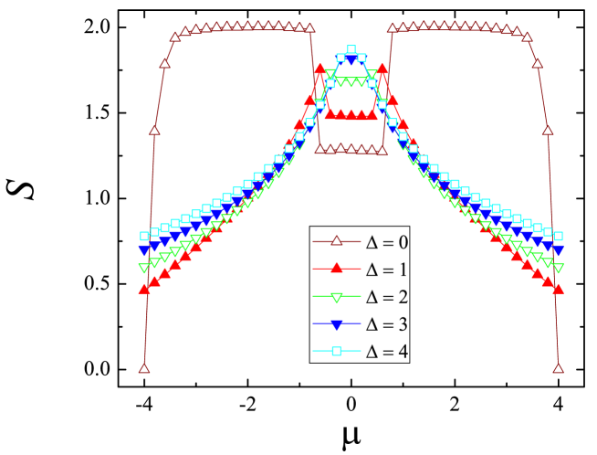
Figure 6: Half-chain entanglement entropy versus $\mu$ for several values of the pairing $\Delta$. We have set the parameters to $t=1$, $U=4$ and $\chi=100$.

In addition, using a conformal scaling with $\chi$,

$$S=\frac{1}{\sqrt{\frac{12}{c}}+1}\ln\chi+\tilde{s},$$

one can determine the central charge $c$ [30] in all critical phases [31] with a constant $\tilde{s}$. In Fig. 7, we present the finite-$\chi$ scaling of the half-chain entanglement entropy for several $\Delta$ and $\mu$. For parameters $U=4$, $\Delta=2$ and $\mu=0.6$, we observe the saturation of $S$ at large $\chi$, a behavior characteristic of a fully gapped phase as expected for the superconducting one. In contrast, for the model with $U=4$, $\Delta=2$ and $\mu=0$, the above conformal scaling is well realized providing the central charge is set to $c=1$, as expected for a Mott phase with a single gapless spin mode.

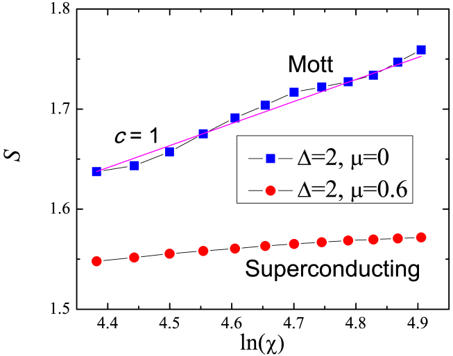
Figure 7: Entanglement entropy versus $\ln(\chi)$ for two values of $\mu$, fixing $U=4$ and $\Delta=2$. For $\mu=0.6$, $S$ saturates at large $\chi$, in agreement with a gapped superconducting behavior. At $\mu=0$, the data can be fitted as $S=0.22\ln(\chi)+\tilde{s}$, in agreement with the conformal scaling with central charge $c=1$ (see text).

In order to provide a complementary quantitative analysis, we have used finite-size DMRG algorithm [32] keeping up to $m=4000$ states and with a discarded weight below $10^{-8}$. For a finite-system with open boundary conditions, conformal field theory [29] predicts that, in a critical region, the block entanglement entropy $S$ should follow the universal scaling behavior:

$$S=\frac{c}{6}\ln d(x|L)+\tilde{s}.$$ (21)

where $c$ is the central charge, $d(x|L)=\pi/L\sin(x\pi/L)$ is the conformal block size of size $x$, and $\tilde{s}$ is a non-universal constant.

In Fig. 8, we present the finite-size scaling of the entanglement entropy for $U=4$ in all different regions. In the metallic phase ($\Delta=0$, $\mu=2$), we measure a large central charge $c\simeq 2$ corresponding to two gapless modes (one in the charge channel, one in the spin channel) as expected. For $\Delta=2$ and $\mu=2$, we are in the fully gapped superconducting phase. Last, in the Mott phase at or close to half-filling (for instance $\Delta=2$ and $\mu=0$), we observe a smooth crossover from a large central charge $c\simeq 2$ at small distance to a proper $c=1$ at large distance, as expected from a single gapless spin mode, as found for instance in the pure Hubbard model with $\Delta=0$. Indeed, it is well-known that, for the pure Hubbard model at half-filling, the charge gap is exponentially small ($\sim\exp(-t/U)$) while it becomes of order $U$ at large $U$ [18]. Similarly, there is a corresponding length scale (proportional to the inverse of the gap) that governs this crossover.

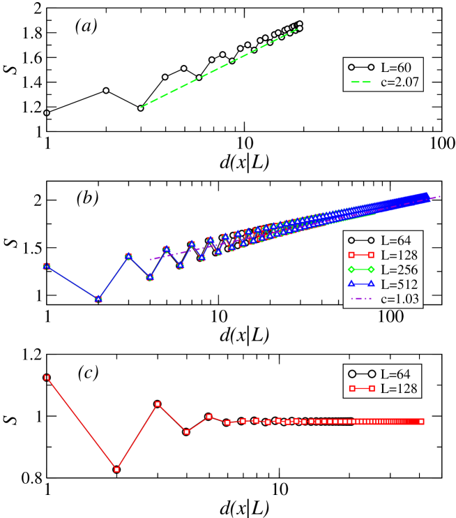
Figure 8: Entanglement entropy scaling versus the conformal size of the block for $U=4$ and various parameters $\Delta$ and $\mu$, obtained from DMRG on chains of length $L$. (a) $\Delta=0$ and $\mu=2$ in the metallic phase; (b) $\Delta=2$ and $\mu=0$ in the Mott phase; (c) $\Delta=2$ and $\mu=2$ in the superconducting phase.

In conclusion on this section, our finite-size DMRG calculations have confirmed that the charge channel is always gapped for finite $\Delta$. However, we have distinguished the Mott phase from the fully gapped superconducting one by its gapless $c=1$ spin mode. Also, we have not seen any clear sign of an intermediate BOW phase with spontaneous translation symmetry breaking, which in principle is allowed as discussed in the Appendix.

4 Conclusion

In summary, we have used both the finite-size and infinite DMRG to obtain the ground-state of the one-dimensional Hubbard model with an additional singlet pairing potential. Such a model would be relevant for a strongly correlated chain with some proximity coupling to a singlet superconductor. We have computed local quantities as well as entanglement properties in order to establish the full phase diagram, including Mott, metallic and superconducting phases.

Our study has revealed a particularly interesting feature of the Mott and superconducting phases, connected to the existence of a potential breaking explicitly particle number conservation. In that case, the inverse of the compressibility $\kappa$ is no longer related to the many-body charge gap $\Delta_{C}$, as $\kappa^{-1}\sim L\,\Delta_{C}$, so that $\Delta_{C}$ and $\kappa$ could be simultaneously non zero in the thermodynamic limit $L\rightarrow\infty$. Such a remarkable feature is examplified by the Mott and the superconducting phases which are both simultaneously gapped (in the charge sector) and compressible. The Mott phase can however be characterized by the existence of a gapless spin mode (described by a $c=1$ CFT) while the superconducting phase is fully gapped.

It would be an interesting prospect to extend this study to two-dimensional systems, using for instance PEPS formulation that does not suffer from the negative sign problem.

Appendix: Mott Insulator to superconductor transition

In the present appendix, we give a more detailed discussion of the case $\mu\neq 0$ where the $g_{3}$ and $\Omega$ terms of (8)–(10) are computed. A similar competition was discussed in the case of the ionic Hubbard model [33, 34] where three phases were found, a Mott insulator, a Band insulator and a narrow [34] intermediate bond order wave phase. Analogously, in our model, an intermediate $c=0$ bond order wave (BOW) phase with $\langle\phi_{c}\rangle=0$ and $\langle\phi_{s}\rangle=0$ could exist between the Mott insulator (MI) and the superconductor (SC). The MI-BOW transition is a Berezinskii-Kosterlitz-Thouless transition where a gap in the spin modes opens, leading to $\langle\phi_{s}\rangle=0$. The BOW-SC transition only affects the charge sector. Thus, to discuss that transition, we can replace $\cos\sqrt{2}\phi_{s}$ by its expectation value in Eq. (10). At the special point $K_{c}=1/2$, using the rescaling $\phi=\sqrt{2}\phi_{c}$ and $\theta=\theta_{c}/\sqrt{2}$ we can rewrite the low-energy Hamiltonian (8)–(10)

$$H_{c}+H_{cs} = \int\frac{dx}{2\pi}\left[u_{c}(\pi\Pi)^{2}+u_{c}(\partial_{x}\phi)^{2}\right]+\frac{h}{\pi}\int dx\partial_{x}\phi$$ (22)

$$-\frac{2g_{3}}{(2\pi\alpha)^{2}}\int dx\cos 2\phi$$

$$+\frac{2\Omega\langle\cos\sqrt{2}\phi_{s}\rangle}{\pi\alpha}\int dx\cos 2\theta,$$

and introduce the fermion operators

$$\psi_{R}=\frac{e^{i(\theta-\phi)}}{\sqrt{2\pi\alpha}},$$ (23)

$$\psi_{L}=\frac{e^{i(\theta+\phi)}}{\sqrt{2\pi\alpha}},$$ (24)

to obtain [19]

$$H_{c}+H_{cs} = -iu_{c}\int dx(\psi^{\dagger}_{R}\partial_{x}\psi_{R}-\psi^{\dagger}_{L}\partial_{x}\psi_{L})-i\frac{U}{2}\int dx(\psi^{\dagger}_{R}\psi_{L}-\psi^{\dagger}_{L}\psi_{R})$$ (25)

$$-h\int dx(\psi^{\dagger}_{R}\psi_{R}+\psi^{\dagger}_{L}\psi_{L})$$

$$-i\frac{2\mu\Delta\langle\cos\sqrt{2}\phi_{s}\rangle}{\sqrt{t^{2}+\Delta^{2}}}\int dx(\psi^{\dagger}_{R}\psi^{\dagger}_{L}-\psi^{\dagger}_{L}\psi^{\dagger}_{R}).$$

The ground state of the Hamiltonian (25) has been studied in [35]. It has a phase transition point in the Ising universality class, whose order parameter is the BOW order parameter. When $h\neq 0$, a disorder point [36, 37] where charge density wave and BOW correlation functions remain short ranged but display incommensuration [35] exists inside the superconducting phase. The Fourier transforms of these correlation functions present a Lifshitz point [38] where a double peak structure develops. In physical terms, the origin of the disorder point is simply that the doping induced by the chemical potential moves the Fermi wavevector away from $\frac{\pi}{2}$ giving rise to incommensurate modulation of the density wave and bond order wave order parameters. While the fermion density displays no singularity at the disorder point, since $h$ can drive the Ising transition [35], it coupled to the Ising energy density operator. This implies that the fermion density has the same singularity at the Ising critical point as the energy density of the Ising model, i.e. $\langle n_{+}+n_{-}\rangle\sim(h-h_{c})\ln|h-h_{c}|$.

References

References

- [1] S. Sachdev, Quantum Phase Transitions, Cambridge University Press, Cambridge, 2011.
- [2] M.-C. Cha, Phys. Rev. B 98 (2018) 235161.
- [3] J. Eisert, M. Cramer, M. B. Plenio, Rev. Mod. Phys. 82 (2010) 277.
- [4] S. White, Phys. Rev. Lett. 69 (1992) 2863.
- [5] S. Östlund, S. Rommer, Phys. Rev. Lett. 75 (1995) 3537.
- [6] U. Schollwöck, Ann. Phys. 326 (2011) 96.
- [7] D. Pérez-García, F. Verstraete, M. M. Wolf, J. I. Cirac, Quant. Inf. Comp. 8 (2008) 0650.
- [8] G. Vidal, Phys. Rev. Lett. 99 (2007) 220405.
- [9] I. P. McCulloch, arXiv:0804.2509.
- [10] A. Y. Kitaev, Physics-Uspekhi 44, (2001) 131.
- [11] M. F. Parsons, F. Huber, A. Mazurenko, C. S. Chiu, W. Setiawan, K. Wooley-Brown, S. Blatt, M. Greiner, Phys. Rev. Lett. 114 (2015) 213002.
- [12] L. W. Cheuk, M. A. Nichols, M. Okan, T. Gersdorf, V. V. Ramasesh, W. S. Bakr, T. Lompe, M. W. Zwierlein, Phys. Rev. Lett. 114 (2015) 193001.
- [13] W. S. Bakr, J. I. Gillen, A. Peng, S. Folling, M. Greiner, Nature 462 (2009) 74.
- [14] A. Mazurenko, C. S. Chiu, G. Ji, M. F. Parsons, M. Kanasz-Nagy, R. Schmidt, F. Grusdt, E. Demler, D. Greif, M. Greiner, Nature 545 (2017) 462.
- [15] M. Schreiber, S. S. Hodgman, P. Bordia, H. P. Lüschen, M. H. Fischer, R. Vosk, E. Altman, U. Schneider, I. Bloch, Science 21 (2015) 842.
- [16] D. Mitra, P. T. Brown, E. Guardado-Sanchez, S. S. Kondov, T. Devakul, D. A. Huse, P. Schauss, W. S. Bakr, Nat. Phys. 14 (2018) 173.
- [17] C. Yang, A. N. Kocharian, Y. L. Chiang, J. Phys.: Condens. Matter 12 (2000) 7433.
- [18] F. H. L. Essler, H. Frahm, F. Göhmann, A. Klümper, V. E. Korepin, The One-Dimensional Hubbard Model, Cambridge University Press, Cambridge, 2005.
- [19] T. Giamarchi, Quantum Physics in One Dimension, Oxford University Press, Oxford, 2004.
- [20] G. I. Japaridze, A. A. Nersesyan, JETP Lett. 27 (1978) 334.
- [21] V. L. Pokrovsky, A. L. Talapov, Phys. Rev. Lett. 42 (1979) 65.
- [22] N. Laflorencie, E. S. Sorensen, M. S. Chang, I. Affleck, Phys. Rev. Lett. 96 (2006) 100603.
- [23] M. Fabrizio, A. O. Gogolin, Phys. Rev. B 51 (1995) 17827.
- [24] S. Eggert, I. Affleck, Phys. Rev. B 46 (1992) 10866.
- [25] S. Eggert, I. Affleck, Phys. Rev. Lett. 75 (1995) 934 .
- [26] S. Rommer, S. Eggert, Phys. Rev. B 62 (2000) 4370.
- [27] G. Bedürftig, B. Brendel, H. Frahm, R. M. Noack, Phys. Rev. B 58 (1998) 10225.
- [28] P. Sengupta, A. W. Sandvik, D. K. Campbell, Phys. Rev. B 65 (2002) 155113.
- [29] P. Calabrese, J. Cardy, J. Stat. Mech. (2004) P06002.
- [30] A. B. Zamolodchikov, JETP Lett 43 (1986) 730.
- [31] F. Pollmann, S. Mukerjee, A. M. Turner, J. E. Moore, Phys. Rev. Lett. 102 (2009) 255701.
- [32] We have used the ITensor C++ library, available at http://itensor.org for our calculations.
- [33] M. Fabrizio, A. O. Gogolin, A. A. Nersesyan, Nucl. Phys. B 580 (2000) 647 .
- [34] L. Tincani, R. M. Noack, D. Baeriswyl, Phys. Rev. B 79 (2009) 165109.
- [35] E. Orignac, R. Citro, M. Di Dio, S. De Palo, Phys. Rev. B 96, (2017) 014518.
- [36] J. Stephenson, Can. J. Phys. 48 (1970) 1724.
- [37] J. Stephenson, Phys. Rev. B 1 (1970) 4405.
- [38] R. M. Hornreich, M. Luban, S. Shtrikman, Phys. Rev. Lett. 35 (1975) 1678.