Anisotropic Mesh Filtering by Homogeneous MLS Fitting

Abstract

In this paper we present a novel geometric filter, a homogeneous moving least squares fitting-based filter (H-MLS filter), for anisotropic mesh filtering. Instead of fitting the noisy data by a moving parametric surface and projecting the noisy data onto the surface, we compute new positions of mesh vertices as the solutions to homogeneous least squares fitting of moving constants to local neighboring vertices and tangent planes that pass through the vertices. The normals for defining the tangent planes need not be filtered beforehand but the parameters for balancing the influences between neighboring vertices and neighboring tangent planes are computed robustly from the original data under the assumption of quadratic precision in each tangent direction. The weights for respective neighboring points for the least squares fitting are computed adaptively for anisotropic filtering. The filter is easy to implement and has distinctive features for mesh filtering. (1) The filter is locally implemented and has circular precision, spheres and cylinders can be recovered exactly by the filter. (2) The filtered mesh has a high fidelity to the original data without any position constraint and salient or sharp features can be preserved well. (3) The filter can be used to filter meshes with various kinds of noise as well as meshes with highly irregular triangulation.

1 Introduction

Along with the development of 3D scanning devices, triangular meshes have been widely used to represent surface shapes in the fields of geometric modeling, computer graphics and computer vision. Due to the accuracy limitations of data capturing, data loss caused by storage or transmission, etc., geometric models represented by triangular meshes can include noise. Thus, constructing a visually smooth triangular mesh from a noisy input one plays a fundamental role for many disciplines and applications.

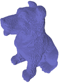
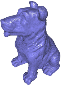
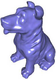
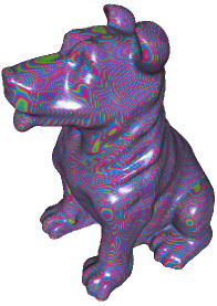
Figure 1: Mesh filtering by H-MLS filter: (a) the surface mesh of a binary voxel model; (b)&(c) meshes after 2 or 5 iterations of filtering; (d) error plot. The purple, green and cyan colors in (d) represent the positive, zero or negative distances from the noisy vertices to the filtered surface. In this paper all noisy and filtered meshes are flat shaded if there is no special declaration.

Many mesh filtering algorithms have been invented by adapting filters for signal processing or techniques for continuous surface smoothing. However, filtering a noisy mesh is more challenging than filtering a 1D or 2D signal or fairing a continuous surface represented by explicit parametric (usually spline) patches. It is more difficult to distinguish sharp features from a noisy mesh than on a piecewise smooth surface. The triangulation of a surface mesh may be highly irregular, direct definition of discrete differential operators on a triangular mesh may be inaccurate. Minor deformation of a filtered signal or image is nearly invisible, but the deformation of a surface mesh can be noticed clearly.

In this paper we present a novel geometric filter for mesh filtering. Figure 1 illustrates an example of mesh filtering by our proposed H-MLS filter. Given a triangulated surface mesh of a binary voxel model, a high fidelity smooth surface is obtained just by a few iterations of filtering without any position constraint. Stairs on original noisy surface have been removed effectively while salient features are preserved perfectly after filtering.

Our proposed technique is motivated by moving least squares (MLS) surface construction from geometric Hermite data [Yang, 2016]. Instead of constructing a smooth parametric surface explicitly, we compute new position of each mesh vertex as the solution to the homogeneous least squares fitting of moving constants to neighboring vertices, tangent planes at the vertices as well as a line passing through or near the original noisy vertex. In order to achieve a high accuracy of approximation, a local shape parameter is introduced to balance the influences between neighboring vertices and neighboring tangent planes. Weights for respective neighboring vertices or planes are used to adapt or control local surface features.

When the filtered vertices are obtained as the solutions to homogeneous moving least squares fitting, the filtering effects depend on the parameters and weights heavily. We use data dependent parameters for high fidelity anisotropic mesh filtering. In order to attenuate the influences of data noise, we compute weights and parameters for least squares fitting from the local geometric data directly under the assumption of quadratic precision in each tangent direction. This filter is flexible enough to recover vertices in smooth surface regions with low or high curvatures as well as vertices lying on sharp edges or corners.

Briefly, the main contributions of the paper are as follows.

• We filter mesh vertices by least squares fitting of moving constants to generalized Hermite data, and the new positions of vertices are directly obtained.

• The weights and parameters for the least squares fitting are chosen for high accuracy approximation or feature preserving filtering.

• The proposed filter is simple but very powerful for filtering meshes with various kinds of noise or triangulation.

The paper is organized as follows. In Section 2 we give a brief review and analysis of existing methods for mesh filtering or denoising. The motivation of the proposed mesh filter is introduced in Section 3 and Section 4 presents the algorithm steps of the new filter. Experimental results are given in Section 5 and the paper is concluded in Section 6 with a brief summary and discussion.

2 Previous work

Lots of algorithms have been proposed for mesh filtering or mesh denoising in the past two decades. According to the basic principles for mesh denoising, the existing algorithms can be roughly classified into four categories.

$\bullet$ Signal processing-based methods. Under the assumption that noises are high frequency signals, many low-pass filters or statistics-based filters for signal or image processing have been generalized to process surface meshes [Taubin, 1995, Alexa, 2002, Peng et al., 2001, Fleishman et al., 2003, Diebel et al., 2006, Sun et al., 2008, Jones et al., 2003]. These methods can usually give visually smooth results, but the challenges are how to distinguish noise from sharp features or how to avoid local or global deformation of the filtered meshes. Practically, a prior step for recognizing features from the noisy data is used for feature-preserving mesh denoising [Shimizu et al., 2005, Fan et al., 2010, Bian and Tong, 2011, Wei et al., 2017].

$\bullet$ PDE or optimization methods. Based on the assumption that a triangular mesh is a discrete approximation of a smooth surface and vertex noise can cause locally high curvatures, techniques based on geometric flows or anisotropic diffusion have been developed for mesh fairing or feature-preserving mesh filtering [Bajaj and Xu, 2003, Clarenz et al., 2000, Hildebrandt and Polthier, 2004, Zhang and Hamza, 2007]. By using $l_{1}$ or $l_{0}$ norm of surface variations as the smoothness measure, sharp features or piecewise flat patches can be recovered [He and Schaefer, 2013, Wu et al., 2015]. When a PDE model has been used for mesh smoothing, proper definition of discrete differential operators plays an important role for the smoothing results [Desbrun et al., 1999, Hildebrandt and Polthier, 2007]. Meshes faired by PDE models can have high quality but may deviate from the original surfaces, one should carefully choose parameters to balance the surface quality and data fidelity [Centin and Signoroni, 2018].

$\bullet$ Normal-guided or data-driven methods. Piecewise smooth normal mapping can help to restore smooth surfaces with feature preserving. Techniques for filtering facet normals and refitting surface meshes to the filtered normals have been studied extensively in recent years [Zhang et al., 2015a, b, Shen and Barner, 2004, Sun et al., 2007, Zheng et al., 2011, Yadav et al., 2018]. Tasdizen, et al. (2003) proposed to filter surface normals by a diffusion equation and refit an implicit surface to the filtered normals. An interesting way is to filter facet normals by data driven-methods [Wang et al., 2016], of which the effects depend much on the quality and amount of training data. Normal filtering does work for mesh denoising, but it is actually a chicken-and-egg problem to filter normals for mesh denoising. Normals of surface meshes constructed from medical image data or binary voxel models may not be filtered correctly by conventional methods. How to avoid flipped edges when refitting triangles to the filtered normals is also a challenge.

$\bullet$ MLS surface fitting methods. Moving least-squares fitting can be used to construct smooth surfaces from noisy input data and the original noisy data can also be filtered by projecting points onto the MLS surface [Lipman et al., 2007, Fleishman et al., 2005, Huang et al., 2013]. For mesh filtering purposes, especially for filtering meshes constructed from medical image data, Wang et al. (2011) proposed to filter mesh vertices by fitting a local quadratic surface to neighborhood of every vertex. Similarly, Wei et al. (2015) employed biquadratic Bézier surfaces for data fitting and point projection. Because a linear system has to be solved for fitting each local surface, how to guarantee the numerical stability and how to improve the computational efficiency have to be considered seriously.

Instead of fitting selected points by moving low-order surface patches, our proposed mesh filter is derived by homogeneous least-squares fitting of moving constants to selected geometric Hermite data. The solutions to the least squares fitting of moving constants can be obtained directly with no need of solving any linear system. By properly chosen parameters for the least squares fitting, points on low or high curvature regions can be restored effectively. Moreover, points on sharp edges or surface meshes with highly irregular triangulation can also be restored very well.

3 Homogeneous MLS Fitting to Geometric Hermite Data

Our proposed mesh filter is motivated by a technique of constructing homogeneous MLS (H-MLS) surfaces from point-normal pairs [Yang, 2016]. Differently from conventional MLS surfaces which fit moving low-order polynomials to points, H-MLS surfaces constructed from point-normal pairs fit moving constants to points and tangent planes at the points. Constructing H-MLS surfaces from point-normal pairs needs not solving any linear system and the obtained surfaces can have circular precision in each tangent direction. Due to its simplicity and high accuracy, the point evaluation scheme for H-MLS surfaces constructed from point-normal pairs will be modified for mesh filtering.

Assume $\{\mathbf{p}_{i}\}_{i=1}^{N}$ are the vertices of a polygon or a surface mesh and $\{\mathbf{n}_{i}\}_{i=1}^{N}$ are unit normal vectors at the points. Assume $\{\xi_{i}\}_{i=1}^{N}$ are the corresponding parameters on a 1D or 2D domain. Let $\phi(\xi)=\phi(|\xi|)$ be a non-negative, symmetric and decreasing function. An H-MLS curve or surface that fits the points and the planes passing through the points with given normals can be obtained by minimizing the following objective function

$$F(\mathbf{p})=\frac{1}{2}\sum_{i=1}^{N}\phi_{i}(\xi)(\mathbf{p}-\mathbf{p}_{i})^{2}+\frac{1}{2}\sum_{i=1}^{N}\mu_{i}\phi_{i}(\xi)[(\mathbf{p}-\mathbf{p}_{i})\cdot\mathbf{n}_{i}]^{2},$$ (1)

where $\phi_{i}(\xi)=\phi(|\xi-\xi_{i}|)$, $i=1,2,\ldots,N$. The parameters $\mu_{i}$s are used to balance the influences of points and lines/planes that pass through the points. When all the parameters satisfy $\mu_{i}>-1$, it is guaranteed that the objective functional $F(\mathbf{p})$ is convex. By minimizing $F(\mathbf{p})$ or solving the equation $\frac{\partial F(\mathbf{p})}{\partial\mathbf{p}}=0$, a curve or surface that fits the original data is obtained as

$$\mathbf{p}=\mathbf{p}(\xi)=\left[\sum_{i=1}^{N}M_{i}\phi_{i}(\xi)\right]^{-1}\sum_{i=1}^{N}M_{i}\mathbf{p}_{i}\phi_{i}(\xi),$$

where $M_{i}=I+\mu_{i}\mathbf{n}_{i}\mathbf{n}_{i}^{T}$, $i=1,2,\ldots,N$, and $I$ is the identity matrix. Figure 2(a) illustrates an H-MLS surface constructed from point-normals which were originally sampled from a torus. Particularly, the points are uniformly parametrized and $\phi(\xi)$ is chosen as the standard bicubic B-spline function. By choosing all $\mu_{i}=1.25$ for defining the functional (1), the obtained H-MLS surface lies closely to the sampled points. As a comparison, if we choose all $\mu_{i}=0$ within the functional, the H-MLS surface reduces to a bicubic B-spline surface; see Figure 2(b).

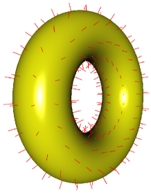
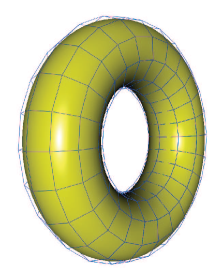
Figure 2: (a) An H-MLS surface constructed from $10\times 20$ point-normal pairs ($\mu_{i}=1.25$). (b) A bicubic B-spline surface with the same set of control points.

Assume the kernel function $\phi(\xi)$ is locally supported, i.e., $\phi(\xi)=0$ when $|\xi|>R$, evaluation of point at a parameter $\xi_{i}$ on the curve or the surface can be simplified. Denote $N(i)=\{j||\xi_{i}-\xi_{j}|\leq R\}$. The point at $\xi=\xi_{i}$ is computed by

$$\hat{\mathbf{p}}_{i}=\mathbf{p}(\xi_{i})=\left[\sum_{j\in N(i)}\omega_{ij}M_{j}\right]^{-1}\sum_{j\in N(i)}\omega_{ij}M_{j}\mathbf{p}_{j},$$ (2)

where $\omega_{ij}=\phi(|\xi_{i}-\xi_{j}|)$. Equation (2) also implies that $\hat{\mathbf{p}}_{i}$ is the solution to a local least squares fitting with weights $\omega_{ij}$ and balance parameters $\mu_{j}$, $j\in N(i)$.

By computing the parameters $\mu_{j}$ under the assumption that the curve $\mathbf{p}(\xi)$ has almost circular or helix precision to the original curve from which the points and normals are sampled, and because smooth curves can be approximated well by smoothly connected circular arcs or helix segments, Equation (2) has been successfully applied for fairing a polygon or a rational spline curve in 2D pr 3D space [Yang, 2018]. In this paper we generalize this technique for filtering surface meshes. However, at least three challenges have to be solved or avoided. First, computing a global parametrization of a general surface mesh is a time consuming step for mesh filtering. Second, the neighborhood of a selected point $\mathbf{p}_{i}$ may not be symmetric and the naively evaluated point may shift on or near the tangent plane that passes through the point. Third, how to preserve salient or sharp features and how to control the fidelity from the filtered mesh to the original one are more challenging.

4 H-MLS Filter for Anisotropic Mesh Filtering

In this section we generalize Equation (2) to filter general types of triangular meshes. Though the weights $\omega_{ij}$ are theoretically dependent on the parametrization of the vertices, we will replace $|\xi_{i}-\xi_{j}|$ by $\|\mathbf{p}_{i}-\mathbf{p}_{j}\|$ or other similar metrics when special properties like feature preserving are desired. In the following we introduce necessary steps and implementation details for our proposed mesh filter.

Before computing new positions for vertices, normal vectors at all mesh vertices are first estimated. Let $N_{T}(i)$ denote the index set of triangles that share a vertex $\mathbf{p}_{i}$. The unit normal vector at the point $\mathbf{p}_{i}$ is computed by

$$\mathbf{n}_{i}=\frac{\sum_{j\in N_{T}(i)}\alpha_{ij}\mathbf{n}_{f_{j}}}{\|\sum_{j\in N_{T}(i)}\alpha_{ij}\mathbf{n}_{f_{j}}\|},$$

where $\mathbf{n}_{f_{j}}$ are the unit normals at the neighboring triangles and $\alpha_{ij}$ are the angles of the triangles at the vertex $\mathbf{p}_{i}$.

$\bullet$ Compute the filtered vertex. We compute the filtered vertex by solving a homogeneous MLS fitting equation. Let $N(i)$ denote the index set of selected neighboring points of vertex $\mathbf{p}_{i}$. We modify the functional (1) to compute optimal new position for vertex $\mathbf{p}_{i}$ as follows

$$F_{i}(\mathbf{p})=\frac{1}{2}\sum_{j\in N(i)}\omega_{ij}(\mathbf{p}-\mathbf{p}_{j})^{2}+\frac{\mu_{i}}{2}\sum_{j\in N(i)}\omega_{ij}[(\mathbf{p}-\mathbf{p}_{j})\cdot\mathbf{n}_{j}]^{2}+\frac{\gamma}{2}[(I-\mathbf{n}_{i}\mathbf{n}_{i}^{T})(\mathbf{p}-\mathbf{p}_{i}^{*})]^{2}.$$ (3)

The first two terms on the right side of Equation (3) represent the squared distances from a point $\mathbf{p}$ to a set of neighboring points as well as the tangent planes at the points. The third term means the squared distance from point $\mathbf{p}$ to the line that passes through $\mathbf{p}_{i}^{*}$ with direction $\mathbf{n}_{i}$. This term can help to keep the filtered vertex lying close to the specified line even when the neighborhood is not symmetric. In this paper we choose $\mathbf{p}_{i}^{*}=\mathbf{p}_{i}$ and $\gamma=1000$ for mesh filtering by default. Figure 3 shows an example of how line constraint can help to preserve the basic triangle shapes of original mesh during filtering. Let $\mathbf{p}_{i}^{center}$ be the centroid of 1-ring neighborhood of $\mathbf{p}_{i}$. We can also choose $\mathbf{p}_{i}^{*}=\mathbf{p}_{i}^{center}$ for vertex filtering, which will lead to a smooth mesh with more uniform triangulation in the end.

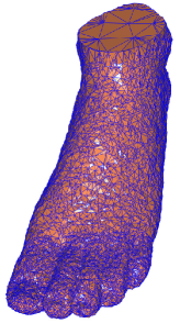
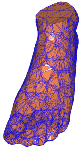
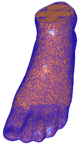
Figure 3: Left: the input noisy mesh; middle & right: meshes filtered by 3 iterations of H-MLS filtering without or with constraint of lines through vertices.

Under the assumption that all weights $\omega_{ij}$ and the parameter $\mu_{i}$ are already known, the derivative of the functional $F_{i}(\mathbf{p})$ with respect to the variable $\mathbf{p}$ is

$$\frac{\partial F_{i}(\mathbf{p})}{\partial\mathbf{p}}=\sum_{j\in N(i)}\omega_{ij}(\mathbf{p}-\mathbf{p}_{j})+\mu_{i}\sum_{j\in N(i)}\omega_{ij}\mathbf{n}_{j}\mathbf{n}_{j}^{T}(\mathbf{p}-\mathbf{p}_{j})+\gamma(I-\mathbf{n}_{i}\mathbf{n}_{i}^{T})(\mathbf{p}-\mathbf{p}_{i}^{*}).$$ (4)

Let $M_{ij}=\omega_{ij}(I+\mu_{i}\mathbf{n}_{j}\mathbf{n}_{j}^{T})$, $j\in N(i)$, and $M_{i}^{*}=\gamma(I-\mathbf{n}_{i}\mathbf{n}_{i}^{T})$. The solution to equation $\frac{\partial F_{i}(\mathbf{p})}{\partial\mathbf{p}}=0$ is

$$\hat{\mathbf{p}}_{i}=\left[\sum_{j\in N(i)}M_{ij}+M_{i}^{*}\right]^{-1}\left(\sum_{j\in N(i)}M_{ij}\mathbf{p}_{j}+M_{i}^{*}\mathbf{p}_{i}^{*}\right).$$ (5)

We assert that the inverse matrix within Equation (5) can be computed robustly by choosing proper weights and parameters.

Proposition 1.

The matrix $\sum_{j\in N(i)}M_{ij}+M_{i}^{*}$ within Equation (5) is reversible when the weights and parameters satisfy $\omega_{ij}\geq 0$, $j\in N(i)$ but $\sum_{j\in N(i)}\omega_{ij}^{2}>0$, $\mu_{i}>-1$ and $\gamma\geq 0$.

Proof.

Notice that the matrix $\sum_{j\in N(i)}M_{ij}+M_{i}^{*}$ is symmetric. To prove the matrix is reversible, we should just prove that the matrix is positive definite. Assume $\mathbf{x}$ is an arbitrary non-zero vector, a quadratic form is obtained as

$$\begin{array}[]{l}\mathbf{x}^{T}\left[\sum_{j\in N(i)}M_{ij}+M_{i}^{*}\right]\mathbf{x}\\ =\sum_{j\in N(i)}\omega_{ij}(\mathbf{x}^{T}\mathbf{x}+\mu_{i}\mathbf{x}^{T}\mathbf{n}_{j}\mathbf{n}_{j}^{T}\mathbf{x})+\gamma(\mathbf{x}^{T}\mathbf{x}-\mathbf{x}^{T}\mathbf{n}_{i}\mathbf{n}_{i}^{T}\mathbf{x})\\ =\sum_{j\in N(i)}\omega_{ij}(\|\mathbf{x}\|^{2}+\mu_{i}|\mathbf{x}^{T}\mathbf{n}_{j}|^{2})+\gamma(\|\mathbf{x}\|^{2}-|\mathbf{x}^{T}\mathbf{n}_{i}|^{2})\\ >0.\end{array}$$

Since the matrix $\sum_{j\in N(i)}M_{ij}+M_{i}^{*}$ is positive definite, it is reversible. The proposition is proven. ∎

Though an inverse matrix has to be computed for filtering each vertex, the computational cost has not been increased significantly as compared with state of art mesh denoising methods. The inverse of a matrix of order 3 can be computed directly by definition. As explained later, Equation (5) will be used as an efficient filter for mesh filtering by computing proper weights and parameters from the original data.

$\bullet$ Compute the parameter $\mu_{i}$. From Equations (3) and (5) we know that the parameter $\mu_{i}$ plays a key role for computing a high fidelity filtered vertex. The mesh vertex may be over smoothed when $\mu_{i}$ has been chosen a small value. A large value of the parameter may push the filtered vertex toward the tangent planes of neighboring vertices. The parameter $\mu_{i}$ should be adaptive to local shape to prevent the filtered mesh from local deformation but it should also be robust enough against data noise for mesh filtering.

We propose to compute the value of $\mu_{i}$ based on the assumption that $\hat{\mathbf{p}}_{i}=\mathbf{p}_{i}$ when the mesh is noise free, irrespective of the point $\mathbf{p}_{i}$ lying on a smooth region or on a sharp feature. Denote by $F^{\prime}_{i}(\mathbf{p}_{i})$ the derivative of the functional $F_{i}(\mathbf{p})$ at $\mathbf{p}=\mathbf{p}_{i}$. The scalar product between $\mathbf{n}_{i}$ and $F^{\prime}(\mathbf{p}_{i})$ is obtained as

$$\mathbf{n}_{i}^{T}F^{\prime}_{i}(\mathbf{p}_{i})=\sum_{j\in N(i)}\omega_{ij}\mathbf{n}_{i}^{T}(\mathbf{p}_{i}-\mathbf{p}_{j})+\mu_{i}\sum_{j\in N(i)}\omega_{ij}\mathbf{n}_{i}^{T}\mathbf{n}_{j}\mathbf{n}_{j}^{T}(\mathbf{p}_{i}-\mathbf{p}_{j}).$$

From equation $\mathbf{n}_{i}^{T}F^{\prime}_{i}(\mathbf{p}_{i})=0$, we have

$$\mu_{i}=\frac{\sum_{j\in N(i)}\omega_{ij}\mathbf{n}_{i}^{T}(\mathbf{p}_{i}-\mathbf{p}_{j})}{\sum_{j\in N(i)}\omega_{ij}\mathbf{n}_{i}^{T}\mathbf{n}_{j}\mathbf{n}_{j}^{T}(\mathbf{p}_{j}-\mathbf{p}_{i})}.$$ (6)

Though the parameter $\mu_{i}$ computed by above equation can be used to recover vertices on a noise-free mesh, the values of $\mu_{i}$ may vary much from vertex to vertex when the mesh data are noisy. A noise sensitive parameter cannot be used for mesh filtering.

To compute a robust value for the parameter $\mu_{i}$, every term in Equation (6) should be computed in a robust way. For a surface mesh the normal curvature at vertex $\mathbf{p}_{i}$ along an edge $\mathbf{p}_{i}\mathbf{p}_{j}$ can be estimated by an osculating arc that interpolates the end points and normal vector $\mathbf{n}_{i}$ at $\mathbf{p}_{i}$, i.e. $k_{ij}^{n}=\frac{2\mathbf{n}_{i}^{T}(\mathbf{p}_{i}-\mathbf{p}_{j})}{\|\mathbf{p}_{i}-\mathbf{p}_{j}\|^{2}}$; see, for example [Meyer et al., 2003]. It yields that $\mathbf{n}_{i}^{T}(\mathbf{p}_{i}-\mathbf{p}_{j})=\frac{1}{2}k_{ij}^{n}\|\mathbf{p}_{i}-\mathbf{p}_{j}\|^{2}$. Similarly, we have $\mathbf{n}_{j}^{T}(\mathbf{p}_{j}-\mathbf{p}_{i})=\frac{1}{2}k_{ji}^{n}\|\mathbf{p}_{j}-\mathbf{p}_{i}\|^{2}$. If $\mathbf{p}_{i}$ and $\mathbf{p}_{j}$ lie closely on a curvature continuous surface, the normal curvatures at the two points satisfy $k_{ij}^{n}\approx k_{ji}^{n}$. It follows that $\mathbf{n}_{i}^{T}(\mathbf{p}_{i}-\mathbf{p}_{j})\approx\mathbf{n}_{j}^{T}(\mathbf{p}_{j}-\mathbf{p}_{i})$. For a mesh vertex lying on a non-convex region the normal curvatures to neighboring vertices may have different signs. Even if the mesh is free of noise, the algebraic sum of the denominator within Equation (6) may still be close to zero or vanish. To keep the denominator from being a small value or zero and to compute the parameter against data noise, we replace both the terms $\mathbf{n}_{i}^{T}(\mathbf{p}_{i}-\mathbf{p}_{j})$ and $\mathbf{n}_{j}^{T}(\mathbf{p}_{j}-\mathbf{p}_{i})$ within Equation (6) by

$$d_{ij}=\max\{\frac{1}{2}(|\mathbf{n}_{i}^{T}(\mathbf{p}_{i}-\mathbf{p}_{j})|+|\mathbf{n}_{j}^{T}(\mathbf{p}_{j}-\mathbf{p}_{i})|),\eta\},$$ (7)

where $\eta>0$ is a small given number. In our experiments we choose $\eta=0.001l_{e}$, where $l_{e}$ is the average edge length of the mesh. By the same way, we replace the term $\mathbf{n}_{i}^{T}\mathbf{n}_{j}$ within Equation (6) by $c_{ij}=\max\{\mathbf{n}_{i}^{T}\mathbf{n}_{j},0.001\}$ which also keeps the denominator positive. Now, the parameter $\mu_{i}$ can be computed robustly as

$$\mu_{i}=\frac{\sum_{j\in N(i)}\omega_{ij}d_{ij}}{\sum_{j\in N(i)}\omega_{ij}c_{ij}d_{ij}}.$$ (8)

The parameter computed by Equation (8) is definitely positive and it is equal to the value computed by Equation (6) when every pair of normal curvatures $k_{ij}^{n}$ and $k_{ji}^{n}$ are equal with each other. Thus, a mesh vertex can be recovered exactly by Equation (5) when its neighboring vertices and normals are uniformly sampled from a sphere or cylinder. This property is important and a filtered surface mesh almost suffers no shrinkage or deformation even without any position constraint.

$\bullet$ Choose kernels and compute weights. As our proposed mesh filtering scheme can be considered a discrete analogy of kernel based MLS surface construction from an arbitrary topology triangular mesh that may have noisy vertices and noisy normals, the smoothness of the filtered mesh depends heavily on the properties of the kernel function. In this paper we choose Gaussian function $\phi(\xi)=\exp(-\frac{\xi^{2}}{2\sigma^{2}})$ as the basic kernel function.

Based on the chosen kernel function, there are two ways to compute the weights for vertex filtering. (1) Weights for isotropic filtering. As discussed in Section 3 and the start of this section, a direct way to compute the weights is $\omega_{ij}=\exp(-\frac{\|\mathbf{p}_{i}-\mathbf{p}_{j}\|^{2}}{2\sigma_{r}^{2}})$, where $\sigma_{r}$ is a user specified number. This choice of weights is useful to remove noise, but sharp features of the mesh are also smoothed out. (2) Weights for anisotropic filtering. To preserve salient or sharp features during filtering, we can choose the weights $\omega_{ij}=\exp(-\frac{d_{ij}^{2}}{2\sigma_{s}^{2}})$, where $d_{ij}$ are computed by Equation (7) and $\sigma_{s}$ is another parameter specified by users. From its definition we know that $d_{ij}=\frac{1}{4}(|k_{ij}^{n}|+|k_{ji}^{n}|)\|\mathbf{p}_{i}-\mathbf{p}_{j}\|^{2}$. By this choice of weights, a mesh is smoothed much more along a feature direction (usually with absolute minor curvature) than across a feature direction. As a result, salient or even sharp features can be preserved well after vertex filtering. In this paper we use the second choice of weights for anisotropic mesh filtering.

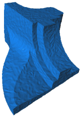
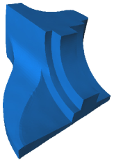
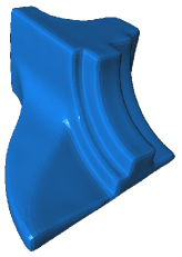
Figure 4: Left: noisy mesh with uniformly distributed noise in normal directions (max. deviation $\pm 10\%l_{e}$); middle: 5 iterations by the proposed filter with $\sigma_{s}=0.05l_{e}$; right: 5 iterations by the proposed filter with $\sigma_{s}=0.2l_{e}$.

The two parameters $\sigma_{r}$ and $\sigma_{s}$ can be chosen depending on the vertex density and noise magnitudes of a noisy mesh. When $\sigma_{r}$ has been specified, at most $m$ nearest points within a sphere centered at a current vertex with radius $R=2\sigma_{r}$ are chosen as the neighborhood of the vertex. The number $m$ is used to balance the computational costs and filtering effects. In our experiments we choose $m=100$ by default for high quality filtering effects and reasonable computational costs. As to the choice of the parameter $\sigma_{s}$, a half of the maximum noise magnitude can be used for feature preserving mesh filtering very well. Mesh noise may not be filtered when $\sigma_{s}$ has been set too small a value, but sharp feature edges or sharp corners will be rounded when $\sigma_{s}$ has been chosen a large one. Figure 4 illustrates an example of mesh filtering with sharp edge preserving or edge and corner rounding by choosing different values for the parameter $\sigma_{s}$. The capability of edge and corner rounding can be used to construct smooth surfaces from rough initial meshes.

Input: Vertex $\mathbf{p}_{i}$ and its neighborhood $\{(\mathbf{p}_{j},\mathbf{n}_{j})\}_{j\in N(i)}$.

Output: New vertex position $\hat{\mathbf{p}}_{i}$.

// sub_routine: Compute_weights_and_parameters;

$s_{a}=0$; $s_{b}=0$ ;

for each neighbor vertex $\mathbf{p}_{j}$ do

      $c_{ij}=\max\{\mathbf{n}_{i}^{T}\mathbf{n}_{j},0.001\}$;

      $d_{ij}=\max\{\frac{1}{2}(|\mathbf{n}_{i}^{T}(\mathbf{p}_{i}-\mathbf{p}_{j})|+|\mathbf{n}_{j}^{T}(\mathbf{p}_{j}-\mathbf{p}_{i})|),\eta\}$;

      $\omega_{ij}=\exp(-\frac{d_{ij}^{2}}{2\sigma_{s}^{2}})$;

      $s_{a}+=\omega_{ij}d_{ij}$;

      $s_{b}+=\omega_{ij}c_{ij}d_{ij}$;

     

      end for

     $\mu_{i}=s_{a}/s_{b}$;

      // main_routine: Compute_the_filtered_vertex;

      $M_{sum}=0$; $\mathbf{p}_{sum}=0$;

      for each neighbor vertex $\mathbf{p}_{j}$ do

           $M_{ij}=\omega_{ij}(I+\mu_{i}\mathbf{n}_{j}\mathbf{n}_{j}^{T})$;

           $M_{sum}+=M_{ij}$;

           $\mathbf{p}_{sum}+=M_{ij}\mathbf{p}_{j}$;

          

           end for

          $M_{i}^{*}=\gamma(I-\mathbf{n}_{i}\mathbf{n}_{i}^{T})$;

           $M_{sum}+=M_{i}^{*}$;

           $\mathbf{p}_{sum}+=M_{i}^{*}\mathbf{p}_{i}^{*}$;

           return $\hat{\mathbf{p}}_{i}=M_{sum}^{-1}\mathbf{p}_{sum}$;

Algorithm 1 H-MLS Filter For Vertex Filtering

So far we have presented all necessary steps for our proposed filter that filter one mesh vertex. The algorithm steps are summarized in Algorithm 1. When all vertices of a mesh have been repositioned by the proposed algorithm, normals at mesh vertices are recomputed for next iteration of vertex filtering. Usually, a few iterations can lead to satisfying results.

5 Results

Our proposed mesh filtering algorithm was implemented using C++ on a double 2.90Ghz Intel(R) Core(TM) CPU with 8G of RAM. We have applied the filter for filtering meshes with several different types of noise. Besides meshes with ordinary triangles, the original mesh can also have highly irregular triangulation or piecewise flat patches. The parameters and time costs for the experimental results are summarized in Table 1.

Table 1: Parameters and time costs for the examples by the proposed algorithm.

Model	Figure	#Vertex	$\frac{R}{l_{e}}$	$\frac{\sigma_{s}}{l_{e}}$	#iter.	Time
Dog	1(c)	208k	3.6	0.4	5	56s
Bunny	5	35k	2	0.25	10	9s
Face	6(e)	41k	2	0.08	4	8s
Retina	7(c)	140k	3.6	0.6	5	36s
Wrench	8(f)	6k	2	0.08	5	2s
Body	9(b)	45k	3.6	0.5	5	12s

Note: The times do not include the time to load meshes or to compute curvatures.

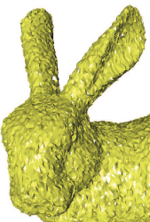
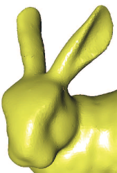
Figure 5: (a) The mesh corrupted by Gaussian noise in randomly chosen directions ($\sigma=0.5l_{e}$); (b)&(c) H-MLS($\mathbf{p}_{i}^{*}=\mathbf{p}_{i}$); (d)&(e)H-MLS($\mathbf{p}_{i}^{*}=\mathbf{p}_{i}^{center}$). The filtered meshes in (c) and (e) are Phong shaded to check the flipped edges or folded triangles.

Figure 5(a) illustrates a bunny model corrupted with Gaussian noise in randomly chosen directions. Consequently, the corrupted mesh has many folded triangles. When the noisy mesh is filtered by our proposed H-MLS filter under the constraint of lines passing through noisy vertices, the mesh has been made smooth but folded triangles still exist; see Figures 5(b)&(c). If we filter the noisy mesh under the constraint of lines passing through 1-ring centroids, the obtained surface is visually smooth and suffers no triangle folding any more; see Figures 5(d)&(e) for the result. In the following we filter vertices under the constraint of lines passing through noisy vertices or 1-ring centroids according to the criterion that the triangle shapes are to be preserved or more smooth results are desired.

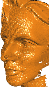
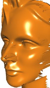
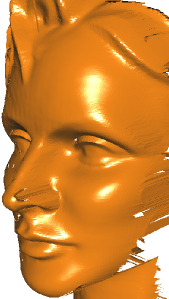
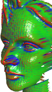
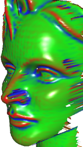
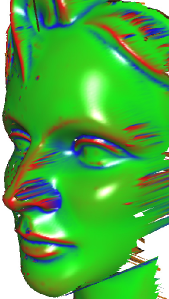
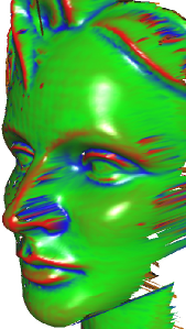
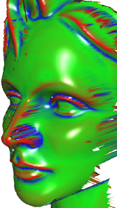
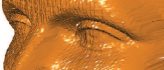
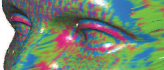
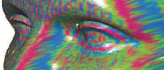
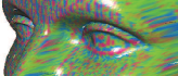
Figure 6: (a) The input noisy mesh; (b) PMC; (c) BMF; (d) BNF; (e) proposed($\mathbf{p}_{i}^{\ast}=\mathbf{p}_{i}$). Middle row: mean curvature plots, where the red color represents the highest value while the blue color means the lowest. Bottom row: error plots for a selected region.

Figure 6 shows a real scan-reconstructed triangular mesh of a face. We have compared our filtering result with those by prescribed mean curvature (PMC) flow [Hildebrandt and Polthier, 2004], bilateral mesh denoising (BMF) [Fleishman et al., 2003] or bilateral normal filtering (BNF) [Zheng et al., 2011]. Similar to ours, these three methods are conceptually simple and can preserve salient features with no complex pre-computation or costly optimization steps. Particularly, the parameters for each known method are chosen carefully to achieve best filtering results. To visualize the surface features and the filtering results clearly, the mean curvature plots of the meshes before or after filtering are computed by employing the method in [Goldfeather and Interrante, 2004]. From the figure we see that both PMC and BNF can preserve or even sharpen local features (e.g. eyelids), but the obtained meshes still suffer low frequency noises in non-feature regions. The BMF can give a smooth filtering result in non-feature regions but minor features have been over smoothed due to the well known shrinkage property of the method. Our proposed method can overcome these shortcomings effectively, a high fidelity filtered mesh with neither over-smoothed areas nor sharpened features is obtained.

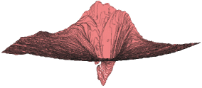
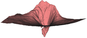
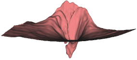
Figure 7: (a) The original mesh; (b) high fidelity mesh denoising [Yadav et al., 2019] (the original and the filtered meshes courtesy of S.K.Yadav); (c) proposed ($\mathbf{p}_{i}^{\ast}=\mathbf{p}_{i}^{center}$).

Figure 7 shows a mesh of a human retina constructed from medical image data. The original surface has many undesired stairs due to limited precision of the marching cubes algorithm. Most noises and minor stairs have been successfully removed by a high fidelity denoising algorithm proposed by Yadav et al. (2019), but stairs at large steps are still visible. Instead of using hard position constraint, we filter the noisy mesh by our proposed H-LMS filter with weights and parameters adaptively computed from the noisy data. By choosing properly sized neighborhood for mesh vertex filtering, a visually smooth surface with neither minor step stairs nor large ones is obtained.

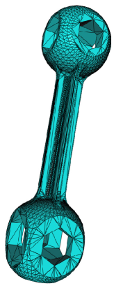
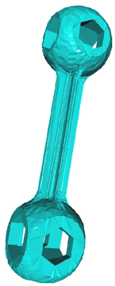
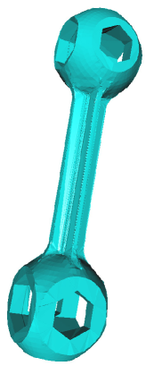
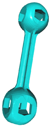
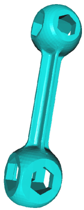
Figure 8: (a) The ground truth model and its triangulation; (b) The mesh corrupted by uniformly distributed noise in normal directions (max. deviation $\pm 10\%l_{e}$); (c) BMF; (d) BNF; (e) proposed($\mathbf{p}_{i}^{\ast}=\mathbf{p}_{i}$).

Figure 8 illustrates a mesh of a CAD model. The original mesh contains highly irregular triangles and the surface is consisting of piecewise smooth patches together with sharp features. From the figure we can see that our proposed filter can almost recover the original mesh exactly. As a comparison, there still exist flipped edges on the meshes denoised by BMF or BNF due to the existence of long and thin triangles.

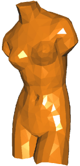
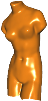
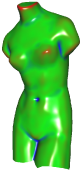
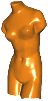
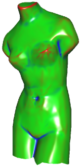
Figure 9: Constructing a smooth surface by filtering a linearly subdivided mesh: (a) the mesh after 3 iterations of binary linear subdivision; (b) result by the proposed filter($\mathbf{p}_{i}^{\ast}=\mathbf{p}_{i}^{center}$); (c) the mean curvature plot of (b); (d) the mesh obtained by linear filtering; (e) mean curvature plot of (d).

Besides filtering a noisy mesh, our proposed filter can also be used to construct smooth surfaces from a rough mesh. Figure 9(a) illustrates a triangular mesh obtained by 3 times of linear binary subdivision. A visually smooth surface is obtained by 5 iterations of H-LMS filtering. The curvature plot also demonstrates the quality of the smoothed mesh. See Figure 9(b)&(c) for the result. As a comparison, if we filter the linearly subdivided mesh by a linear filter, the obtained surface is no longer as fair as expected. See Figure 9(d)&(e) for the surface obtained by 10 iterations of $\lambda|\mu$ algorithm [Taubin, 1995]. We note that discrete fair surfaces can also be constructed by some optimization techniques, e.g. [Schneider and Kobbelt, 2001, Crane et al., 2013]. Even though, our proposed filter owns the advantages of simplicity and efficiency for fair surface modeling.

6 Conclusions and discussion

In this paper we have presented a simple but effective filter for anisotropic mesh filtering. Particularly, new positions of mesh vertices are computed by homogeneous least-squares fitting of moving constants to Hermite data. Curvature-aware parameters and weights for the least squares fitting have been robustly computed from the noisy data. The proposed filter can be used to filter meshes with various kinds of noise as well as meshes with highly irregular triangulation. The filtered mesh has high quality as well as high fidelity to the original data. Smooth surfaces with various curvatures can be restored from noisy meshes effectively by the proposed filter. Sharp features with discontinuous normals can also be preserved well when the noise magnitudes are not high.

Limitations. Our proposed filter can be used to filter meshes with locally high curvatures but free of sharp features or meshes having sharp features but with only low magnitudes noise very well. If the sharp features of a noisy mesh cannot be distinguished from high-magnitude noise locally, our proposed filter no longer preserves sharp features.

Future work. At present we filter meshes with no need of filtering normals beforehand. Combining the filter with other geometric processing techniques such as robust normal estimation or feature detection, etc. will give more impressive results. We focus on mesh filtering in this paper, another interesting future work is to adapt the proposed filter for point set surface processing.

References

- Alexa [2002] Alexa, M., 2002. Wiener filtering of meshes, in: Shape Modeling International, pp. 51–57.
- Bajaj and Xu [2003] Bajaj, C., Xu, G., 2003. Anisotropic diffusion of surfaces and functions on surfaces. ACM Transactions on Graphics 22, 4–32.
- Bian and Tong [2011] Bian, Z., Tong, R., 2011. Feature-preserving mesh denoising based on vertices classification. Computer Aided Geometric Design 28, 50–64.
- Centin and Signoroni [2018] Centin, M., Signoroni, A., 2018. Mesh denoising with (geo)metric fidelity. IEEE Trans. Vis. Comput. Graph. 24, 2380–2396.
- Clarenz et al. [2000] Clarenz, U., Diewald, U., Rumpf, M., 2000. Anisotropic geometric diffusion in surface processing, in: IEEE Visualization 2000, pp. 397–405.
- Crane et al. [2013] Crane, K., Pinkall, U., Schröder, P., 2013. Robust fairing via conformal curvature flow. ACM Trans. Graph. 32, 61:1–61:10.
- Desbrun et al. [1999] Desbrun, M., Meyer, M., Schröder, P., Barr, A.H., 1999. Implicit fairing of irregular meshes using diffusion and curvature flow, in: Proceedings of SIGGRAPH 1999, ACM. pp. 317–324.
- Diebel et al. [2006] Diebel, J.R., Thrun, S., Bruenig, M., 2006. A Bayesian method for probable surface reconstruction and decimation. ACM Transactions on Graphics 25, 39–59.
- Fan et al. [2010] Fan, H., Yu, Y., Peng, Q., 2010. Robust feature-preserving mesh denoising based on consistent subneighborhoods. IEEE Transactions on Visualization and Computer Graphics 16, 312–324.
- Fleishman et al. [2005] Fleishman, S., Cohen-Or, D., Silva, C.T., 2005. Robust moving least-squares fitting with sharp features. ACM Trans. Graph. 24, 544–552.
- Fleishman et al. [2003] Fleishman, S., Drori, I., Cohon-Or, D., 2003. Bilateral mesh denoising. ACM Transactions on Graphics 22, 950–953.
- Goldfeather and Interrante [2004] Goldfeather, J., Interrante, V., 2004. A novel cubic-order algorithm for approximating principal direction vectors. ACM Transactions on Graphics 23, 45–63.
- He and Schaefer [2013] He, L., Schaefer, S., 2013. Mesh denoising via minimization. ACM Trans. Graph. 32, 64:1–64:8.
- Hildebrandt and Polthier [2004] Hildebrandt, K., Polthier, K., 2004. Anisotropic filtering of non-linear surface features. Computer Graphics Forum 23, 391–400.
- Hildebrandt and Polthier [2007] Hildebrandt, K., Polthier, K., 2007. Constrained-based fairing of surface meshes, in: Proceedings of Eurographics symposium on geometry processing, pp. 203–212.
- Huang et al. [2013] Huang, H., Wu, S., Gong, M., Cohen-Or, D., Ascher, U.M., Zhang, H.R., 2013. Edge-aware point set resampling. ACM Trans. Graph. 32, 9:1–9:12.
- Jones et al. [2003] Jones, T.R., Durand, F., Desbrun, M., 2003. Non-iterative, feature preserving mesh smoothing. ACM Transactions on Graphics 22, 943–949.
- Lipman et al. [2007] Lipman, Y., Cohen-Or, D., Levin, D., 2007. Data-dependent MLS for faithful surface approximation, in: Proceedings of the Fifth Eurographics Symposium on Geometry Processing, Barcelona, Spain, July 4-6, 2007, pp. 59–67.
- Meyer et al. [2003] Meyer, M., Desbrun, M., Schröder, P., Barr, A.H., 2003. Discrete differential-geometry operators for triangulated 2-manifolds, in: Visualization and Mathematics III, pp. 35–57.
- Peng et al. [2001] Peng, J., Strela, V., Zorin, D., 2001. A simple algorithm for surface denoising. Tech. Rep.
- Schneider and Kobbelt [2001] Schneider, R., Kobbelt, L., 2001. Geometric fairing of irregular meshes for free-form surface design. Computer Aided Geometric Design 18, 359–379.
- Shen and Barner [2004] Shen, Y., Barner, K.E., 2004. Fuzzy vector median-based surface smoothing. IEEE Transactions on Visualization and Computer Graphics 10, 252–265.
- Shimizu et al. [2005] Shimizu, T., Date, H., Kanai, S., Kishinami, T., 2005. A new bilateral mesh smoothing method by recognizing features, in: Proceedings of the Ninth International Conference on Computer Aided Design and Computer Graphics, pp. 281–286.
- Sun et al. [2007] Sun, X., Rosin, P.L., Martin, R.R., Langbein, F.C., 2007. Fast and effective feature-preserving mesh denoising. IEEE Transactions on Visualization and Computer Graphics 13, 925–938.
- Sun et al. [2008] Sun, X., Rosin, P.L., Martin, R.R., Langbein, F.C., 2008. Random walks for feature preserving mesh denoising. Computer Aided Geometric Design 25, 437–456.
- Tasdizen et al. [2003] Tasdizen, T., Whitaker, R., Burchard, P., Osher, S., 2003. Geometric surface processing via normal maps. ACM Transactions on Graphics 22, 1012–1033.
- Taubin [1995] Taubin, G., 1995. A signal processing approach to fair surface design, in: Proceedings of SIGGRAPH 1995, ACM. pp. 351–358.
- Wang and Yu [2011] Wang, J., Yu, Z., 2011. Quality mesh smoothing via local surface fitting and optimum projection. Graphical Models 73, 127–139.
- Wang et al. [2016] Wang, P., Liu, Y., Tong, X., 2016. Mesh denoising via cascaded normal regression. ACM Trans. Graph. 35, 232:1–232:12.
- Wei et al. [2017] Wei, M., Liang, L., Pang, W., Wang, J., Li, W., Wu, H., 2017. Tensor voting guided mesh denoising. IEEE Trans. Automation Science and Engineering 14, 931–945.
- Wei et al. [2015] Wei, M., Zhu, L., Yu, J., Wang, J., Pang, W., Wu, J., Qin, J., Heng, P., 2015. Morphology-preserving smoothing on polygonized isosurfaces of inhomogeneous binary volumes. Computer-Aided Design 58, 92–98.
- Wu et al. [2015] Wu, X., Zheng, J., Cai, Y., Fu, C., 2015. Mesh denoising using extended ROF model with fidelity. Comput. Graph. Forum 34, 35–45.
- Yadav et al. [2018] Yadav, S.K., Reitebuch, U., Polthier, K., 2018. Mesh denoising based on normal voting tensor and binary optimization. IEEE Trans. Vis. Comput. Graph. 24, 2366–2379.
- Yadav et al. [2019] Yadav, S.K., Reitebuch, U., Polthier, K., 2019. Robust and high fidelity mesh denoising. IEEE Trans. Vis. Comput. Graph. 25, 2304–2310.
- Yang [2016] Yang, X., 2016. Matrix weighted rational curves and surfaces. Computer Aided Geometric Design 42, 40–53.
- Yang [2018] Yang, X., 2018. Fitting and fairing Hermite-type data by matrix weighted NURBS curves. Computer-Aided Design 102, 22–32.
- Zhang et al. [2015a] Zhang, H., Wu, C., Zhang, J., Deng, J., 2015a. Variational mesh denoising using total variation and piecewise constant function space. IEEE Trans. Vis. Comput. Graph. 21, 873–886.
- Zhang et al. [2015b] Zhang, W., Deng, B., Zhang, J., Bouaziz, S., Liu, L., 2015b. Guided mesh normal filtering. Comput. Graph. Forum 34, 23–34.
- Zhang and Hamza [2007] Zhang, Y., Hamza, A.B., 2007. Vertex-based diffusion for 3d mesh denoising. IEEE Transactions on Image Processing 16, 1036–1045.
- Zheng et al. [2011] Zheng, Y., Fu, H., Au, O.K.C., Tai, C.L., 2011. Bilateral normal filtering for mesh denoising. IEEE Transactions on Visualization and Computer Graphics 17, 1521–1530.