Unveiling the importance of magnetic fields in the evolution of dense clumps formed at the waist of bipolar H ii regions: a case study on Sh2-201 with JCMT SCUBA-2/POL-2

Abstract

We present the properties of magnetic fields (B-fields) in two clumps (clump 1 and clump 2), located at the waist of the bipolar H ii region Sh2-201, based on JCMT SCUBA-2/POL-2 observations of 850 $\mu$m polarized dust emission. We find that B-fields in the direction of the clumps are bent and compressed, showing bow-like morphologies, which we attribute to the feedback effect of the H ii region on the surface of the clumps. Using the modified Davis-Chandrasekhar-Fermi method we estimate B-fields strengths of 266 $\mu$G and 65 $\mu$G for clump 1 and clump 2, respectively. From virial analyses and critical mass ratio estimates, we argue that clump 1 is gravitationally bound and could be undergoing collapse, whereas clump 2 is unbound and stable. We hypothesize that the interplay between thermal pressure imparted by the H ii region, B-field morphologies, and the various internal pressures of the clumps (such as magnetic, turbulent, and gas thermal pressure), has the following consequences: (a) formation of clumps at the waist of the H ii region; (b) progressive compression and enhancement of the B-fields in the clumps; (c) stronger B-fields will shield the clumps from erosion by the H ii region and cause pressure equilibrium between the clumps and the H ii region, thereby allowing expanding I-fronts to blow away from the filament ridge, forming bipolar H ii regions; and (d) stronger B-fields and turbulence will be able to stabilize the clumps. A study of a larger sample of bipolar H ii regions would help to determine whether our hypotheses are widely applicable.

=500

1 Introduction

1.1 H ii region feedback and magnetic fields

Massive stars with mass $>$8 M_☉ influence their surroundings via (a) energetic jets and outflows during their initial stages, (b) stellar winds, radiation pressure, and H ii regions (which drive shocks and ionization fronts (I-fronts)) during their intermediate stages, and (c) supernova explosions at the end of their lives (e.g., Tan et al., 2014; Motte et al., 2018). These factors impact the second generation of stars through the resultant injection of energy and momentum into the ambient medium. Stellar feedback has two potential consequences – first by injecting the turbulence into the cloud it stabilizes the cloud against its own gravity and maintains it in a state of quasi-static equilibrium (Krumholz et al., 2005; Krumholz & Tan, 2007; Federrath, 2013); and second, by triggering star formation it reduces the lifetime of a cloud to a few free-fall time scales (Elmegreen, 2007; Dobbs et al., 2011; Vázquez-Semadeni et al., 2009). These effects, which are known as negative and positive feedback, respectively, result in reduced or enhanced levels of star formation in a cloud. The key agents involved in the processes described above include magnetic fields (hereafter B-fields), turbulence, gravity, and H ii region feedback. However the relative importance of B-fields in comparison to the other parameters, and the complex interplay between them is poorly understood.

Deharveng et al. (2015) and Samal et al. (2018) identified several bipolar H ii regions in our Galaxy using Herschel and Spitzer data analyses. They have suggested that such regions form due to the anisotropic expansion of H ii region in flat- or sheet-like filamentary clouds, in accordance with recent 2D numerical simulations (Wareing et al., 2017, 2018). In addition, Samal et al. (2018) found that the most massive and compact clumps are always formed at the waist the bipolar H ii regions (see their Figure 3) showing the signatures of high-mass star formation. Since such clumps are possible sites of massive star and cluster formation, understanding the role of B-fields along with stellar feedback, turbulence, and gravity, as well as the interplay among them holds a key to understand the star formation in such environments. While all other parameters can be relatively well constrained, B-fields are difficult to probe, quantify, and constrain.

Dust grains are believed to be aligned with respect to the B-field orientation via the “radiative alignment torques (RAT)" mechanism (Lazarian, 2007; Lazarian et al., 2015; Andersson et al., 2015). The RAT model predicts that asymmetric, nonspherical dust grains rotate as a result of radiative torques imparted by their local radiation field, and so align themselves with their long axis perpendicular to the ambient B-fields (Dolginov & Mitrofanov, 1976; Draine & Weingartner, 1997; Weingartner & Draine, 2003; Lazarian & Hoang, 2007). The polarized thermal dust emission yields two quantities – the polarization fraction and the polarization position angle, which reveal polarized dust characteristics and the plane-of-sky component of the B-field morphology, respectively.

Several studies have attempted to probe B-fields in regions with stellar feedback using optical, near-infrared, and sub-millimeter polarization observations (Pereyra & Magalhães, 2007; Wisniewski et al., 2007; Kusune et al., 2015; Chen et al., 2017; Pattle et al., 2017; Liu et al., 2018). These studies have demonstrated that initially weak B-fields become stronger as a consequence of feedback-driven compression. These stronger B-fields play a crucial role in the formation and evolution of a variety of structures around H ii regions. Eswaraiah et al. (2017) have carried out NIR polarimetry towards RCW57A, a bipolar H ii region hosting a filament and dense clumps at the waist of H ii region, and found that B-fields are not only important to the formation and evolution of the filamentary cloud, but also strong enough to constrain the flows of expanding I-fronts to form the bipolar H ii regions. However, they could not probe the B-fields in the deeply embedded clumps under the influence of early stellar feedback, due to their heavy extinction. In this study, we probe B-fields in the dense clumps located at the waist of a geometrically simple bipolar H ii region Sh2-201 (hereafter S201).

1.2 Description of Sh2-201

Figure 1: The overall view of the W5-E complex and S201 region. Background image is the color composite of Herschel SPIRE/250 $\mu$m (red; traces cold dust emission), Herschel PACS/100 $\mu$m (green; traces warm dust, mainly from the photodissociation regions (PDRs)), and DSS2-red survey (blue; traces H$\alpha$ emission) images. Various known Bright Rimmed Clouds (BRCs) are shown. This figure is reproduced from Figure 2 of Deharveng et al. (2012) with permission.

S201, with central coordinates of RA (J2000)$=$03^h03^m17$\fs$9, Dec (J2000) $=$ $+$60$\arcdeg$27$\arcmin$52$\arcsec$, is located to the east of the W5-E star-forming complex, as shown in Figure 1. This region is located at a distance of 2 kpc in the Perseus arm (Megeath et al., 2008; Hachisuka et al., 2006). It is a part of an elongated ($\sim$15$\arcmin$) filamentary cloud of mass 3.3$\times$10⁴ M_☉, as seen in ¹³CO (Niwa et al., 2009, see their Figure 1). The local standard of rest velocities (V_LSR) for the clumps of the W5-E region, as well as of S201, lie between $\sim-$38 km s^-1 and $\sim-$40 km s^-1 (Niwa et al., 2009). Similarly, the velocities of radio recombination lines (RRLs) of the ionized gas of S201 (V(RRLs) $=$ $-$34.6 km s^-1, Lockman 1989; V(H$\alpha$) $=$ $-$35.5 km s^-1, Fich et al. 1990) are also in close agreement with those of the molecular gas of W5-E. Based on the distributions of (a) young stellar objects (Class 0, Class I, and Class II) from Spitzer (Koenig et al., 2008) and Herschel (Deharveng et al., 2012) observations, (b) the physical conditions of the cold dust, (c) H ii regions, and (d) exciting OB type stars, Deharveng et al. (2012) suggested that the entire W5-E complex and S201 are formed along a same parental dense, sheet-like, filamentary molecular cloud (see Figure 1). These results corroborate the hypothesis that S201 is a part of W5-E (see Figure 1).

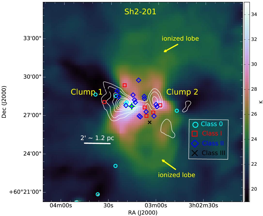
Figure 2: The overall morphology and star formation activity in S201. Background image is the dust temperature map (in units of Kelvin). Column density map is overlaid using white contours at levels of [4, 6, 12, 18, 24, 36, 48, 60, 72, 84]% of the peak column density of 6.94$\times$10²² cm^-2. The Class 0 sources, based on Herschel 100/160 $\mu$m data, are marked with cyan circles (Deharveng et al., 2012). The Class I, II, and III sources, respectively, are marked with square, diamond, and cross symbols (Koenig et al., 2008). Positions of the two clumps, of swept-up matter around the two ionized lobes of the Hii region, and of the ionizing source (green plus) are shown. Both dust temperature and column density maps are provided by Deharveng et al. (2012). A scale length of 2$\arcmin\sim$ 1.2 pc is shown.

Figure 2 shows a zoomed-in view of S201. NIR observations (Ojha et al., 2004) reveal that S201 hosts a compact embedded star cluster containing more than one hundred stars and the most luminous member of the cluster is an O6–O8 zero age main sequence star (green plus symbol; Figures 2, 3, and 5(a)). As can be seen from Figure 2, S201 is made up of two lobes extending from the center of the H ii region and two dense clumps (namely, clump 1 and clump 2) at its waist. Radio, molecular hydrogen, and Br$\gamma$ images have revealed arc-like or bow-like structured photo-dissociation regions at the interface between the H ii region and the clumps, highlighting the interaction between them (Ojha et al., 2004). Several candidate Class 0 and Class I sources have been found within the vicinity of the clumps (Koenig et al., 2008; Deharveng et al., 2012). Since the life-time of Class 0/I YSOs is the order of 10⁵ yr (e.g., Evans et al., 2009), the clumps age is $\lesssim$10⁵ yr. Therefore the clumps are likely to be in the early stages of their evolution, and so ideal candidates for investigating the interplay between B-fields, turbulence, gravity, and thermal pressure, and their implications for the formation and evolution of dense clumps and bipolar H ii regions.

This paper is organized as follows. Section 2 describes JCMT SCUBA-2/POL-2 observations, data reduction, and analyses. This section also presents molecular line (¹³CO and C¹⁸O) data from JCMT/HARP. Results based on the detailed analysis of B-field morphology and correlations between B-fields and intensity gradients (based on the VLA 21cm data) are presented in Section 3. In this section, we also derive various parameters such as dust properties (gas column and number densities, and mass), gas kinematics (velocity dispersion and turbulent pressure), angular dispersion in B-fields (using structure function and auto-correlation function analyses), estimated B-field strength, and ionized gas properties (thermal and radiation pressure). Section 4 discusses the interplay between various parameters, stability analyses based on virial and critical mass estimates, and the consequences for the formation and evolution of clumps, and the formation of bipolar H ii regions. Finally, the conclusions of our current study are summarized in Section 5.

2 Observations and data reduction

2.1 Dust continuum polarization observations using JCMT SCUBA-2/POL-2

Dust continuum polarization observations have been conducted using the POL-2 polarimeter installed on the SCUBA-2 camera (hereafter SCUBAPOL2) at the James Clerk Maxwell Telescope (JCMT; Holland et al. 2013), a 15 m single dish submillimeter observatory located on the summit of Mauna Kea in Hawaii, USA. POL-2 observations of the S201 region (project code: M17BP041; PI: Eswaraiah Chakali) were carried out on 2017 November 18 using the POL-2 DAISY mapping mode (Holland et al., 2013; Friberg et al., 2016). Three sets of observations were acquired under JCMT Band 1 weather conditions, during which the atmospheric optical depth at 225 GHz, $\tau_{225}$, was 0.03. Each set was observed for 30 minutes, resulting in a total integration time of $\sim$1.5 hr.

The POL-2 DAISY scanning mode observes a fully sampled circular region of 15 arcmin diameter. The rms noise is uniform within the central 3$\arcmin$-diameter region of the DAISY map, increasing towards the outer parts of the map. POL-2 data were taken at 450 and 850 $\mu$m simultaneously, with a resolution of 9$\farcs$6 arcsec and 14$\farcs$1, respectively. Here we present the results of 850 $\mu$m data only, due to the low sensitivity of the 450 $\mu$m data. A flux calibration factor (FCF) of 725 Jy pW^-1 beam^-1 was applied to the 850 $\mu$m Stokes I, Q, and U parameters. This FCF value was derived by multiplying the typical SCUBA-2 FCF of 537 Jy pW^-1 beam^-1 (Dempsey et al., 2013) by a transmission correction factor of 1.35 measured in the laboratory and confirmed empirically by the POL-2 commissioning team using observations of Uranus (Friberg et al., 2016).

The POL-2 data were reduced using the Starlink pol2map routine (adapted from the SCUBA-2 data reduction procedure makemap), which was recently added to the Starlink Smurf mapmaking software suite (Berry et al., 2005; Chapin et al., 2013; Currie et al., 2014). To correct for the instrumental polarization at JCMT/850 $\mu$m, we employed the 2018 January IP model during the data reduction, which was extensively tested by the POL-2 commissioning team (Friberg et al., 2016, 2018). Instrumental polarization is typically $\sim$1.5% of the measured total intensity (Friberg et al., 2018). More details on the equations and procedures used to derive the polarization measurements: the debiased degree of polarization [$P$ (%)], polarization angles [$\theta$ ($\arcdeg$)], Stokes parameters [$Q$ (%) and $U$ (%)], intensity [$I$ (mJy/beam)], and polarized intensity [$PI$ (mJy/beam)] along with their uncertainties, can be found in recently-published work (Wang et al., 2019; Coudé et al., 2019; Liu et al., 2019, and references therein).

The final Stokes I, Q, and U maps have a pixel size of 4$\arcsec$; however, the polarization vector catalog was created by setting the bin size parameter in the third step of pol2map to 12$\arcsec$, in order to achieve better sensitivity. The mean rms noise in the Stokes I measurements, $\sigma_{I}$, is $\sim$5 mJy/beam (note that the mean rms noise in the $4\arcsec$ pixel-size Stokes I map is $\sim$14 mJy/beam). In order to infer the B-field orientation in the clumps, we have excluded the data corresponding to fainter regions whose polarization measurements are generally noise-dominated. Therefore, we adopted the following data selection criteria: ratio of intensity to its uncertainty, $I/\sigma_{I}$, $>$ 10; and ratio of polarization fraction to its uncertainty, $P/\sigma_{P}$, $>$ 2, yielding a total of 62 polarization measurements, which are listed, along with their coordinates, in Table 1. We also listed $I$ and $PI$ along with their uncertainties. It should be noted that the $\theta$ values listed have a correction of 90$\arcdeg$, and hence infer the B-field orientation projected on the plane of sky.

In this work, we investigate the morphology and strength of B-fields. Results based on the polarization characteristics and alignment efficiency of the dust grains will be published elsewhere (Eswaraiah et al. in prep), and will consist of various analyses of the relationship between $P$ and $I$ using the POL2 data of S201.

2.2 Molecular lines data from JCMT HARP

The JCMT is also equipped with the Heterodyne Array Receiver Program (HARP)/Auto-Correlation Spectral Imaging System (ACSIS) high-resolution heterodyne spectrometer, capable of observing molecular lines between 325 and 375 GHz (or 0.922 mm and 0.799 mm). HARP is a 4 $\times$ 4 detector array that can be used in combination with ACSIS to rapidly produce large-scale velocity maps of astronomical sources (Buckle et al., 2009). In this paper, we use archival ¹³CO (3–2) and C¹⁸O (3–2) molecular line data ($\sim$14$\arcsec$ resolution, project ID: M09BU04, PI: Mark Thompson, observed on 2009-08-25) to examine the distribution of gas and to extract the gas velocity dispersion values in clumps 1 and 2.

3 Analyses and Results

3.1 B-field morphology

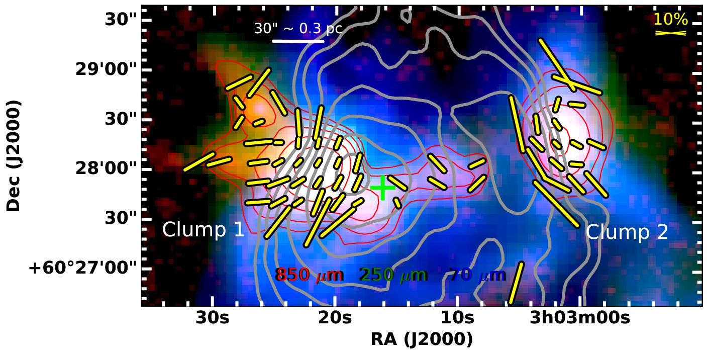
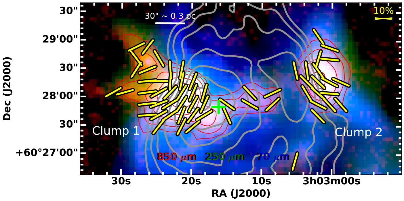
Figure 3: Vector maps showing B-field orientations, lengths proportional to polarization fraction (top panel) and with fixed lengths (bottom panel). B-field vector maps are overlaid on the color composite of JCMT/SCUBAPOL2 850 $\mu$m Stokes I (red), Herschel SPIRE/250 $\mu$m (green), and Herschel PACS/70 $\mu$m (blue) images. Red contours correspond to JCMT/SCUBAPOL2 850 $\mu$m Stokes I map and are drawn at $[$3, 6, 12, 24, 48, 96, 192$]$ $\times$ the rms noise of 14 mJy/beam. Gray contours, corresponding to the VLA/21 cm continuum emission representing the distribution of the ionized medium of H ii region, are drawn at $[$1, 3, 6, 12, 24, 48, 96, 206$]$ $\times$ the rms noise of 2.3$\times$10^-4 mJy/beam (where beam size $\sim 17\arcsec\times 13\arcsec$). In both panels, reference vectors with a B-field orientation of 90$\arcdeg$, along with mean uncertainty of 7$\arcdeg$ are shown.

The measured $P$ values range from $\sim$2% to $\sim$25% with a mean and standard deviation of $\sim$7$\pm$5%, while the B-field orientations ($\theta$) range from $\sim$4$\arcdeg$ to $\sim$177$\arcdeg$ with a mean and standard deviation of $\sim$99$\pm$50$\arcdeg$; a higher standard deviation implies a widely distributed B-field morphology with multiple components. The mean measured uncertainties in $P$ and $\theta$ are $\sim$2$\pm$1% and $\sim$7$\pm$4$\arcdeg$, respectively. The mean uncertainties in Stokes parameters, $\sigma_{I}$, $\sigma_{Q}$, and $\sigma_{U}$, are found to be $\sim$5, $\sim$2, and $\sim$2 mJy beam^-1, respectively. Similarly, the mean uncertainties in polarization ($\sigma_{P}$) and B-field orientation ($\sigma_{\theta}$) are found to be $\sim$2% and $\sim$7$\arcdeg$, respectively.

Our aim is to derive various parameters for the two clumps at the waist of Sh201. We thus separate the polarization data according to the areas covered by individual clumps, and by the ionized medium. Of the 62 total measurements, we find that 36 and 18 are in the direction of clumps 1 and 2, respectively, while the remaining 8 measurements are located between or away from the two clumps, and are excluded assuming that they are not representatives of either clump.

The B-field geometry, based on our 62 measurements, is superimposed on the color composite of POL-2 Stokes I, Herschel/SPIRE 250 $\mu$m, and Herschel/PACS 70 $\mu$m images shown in Figure 3. Red and gray contours correspond to the distributions of dust emission (based on POL-2 850 $\mu$m I map) and of the H ii region (based on VLA 1.45 GHz/21 cm continuum), respectively. Evidently, B-fields in clump 1 follow a bow-like morphology and are conspicuously compressed at the interface region between the dust emission and the ionized medium. This interaction can be witnessed from the closely spaced 21-cm contours. B-fields also seem to be compressed in clump 2 but with a lower degree of curvature.

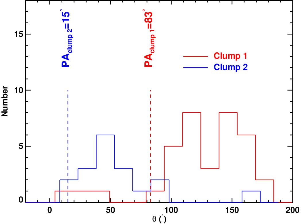
Figure 4: Distributions of B-field orientation of clumps 1 and 2, represented by red and blue histograms, respectively. Position angles of the major axes of clumps 1 and 2 are respectively shown with dashed red and blue lines at 91$\arcdeg$ and 8$\arcdeg$.

Histograms of the B-field orientation, shown in Figure 4, reveal the existence of two major components in clump 1. One component, located near the interaction region of the H ii region and the dust emission (POL2 Stokes I), peaks at $\sim$150$\arcdeg$ and is oriented northwest-southeast. The other component, located on the eastern side of clump 1, is oriented at $\sim$115$\arcdeg$, approximately along the east-west direction, nearly parallel to the major axis (position angle $\sim$83$\arcdeg$) of clump 1. Conversely, the B-fields in clump 2 exhibit a single component with a prominent peak at $\sim$50$\arcdeg$ and is oriented northeast-southwest. This B-field component is neither parallel nor perpendicular to the major axis (position angle of $\sim$15$\arcdeg$) of clump 2. Figures 3 and 4 imply the presence of multiple B-field components in clumps 1 and 2.

3.2 Intensity (ionized gas) gradients versus B-fields

In order to examine whether the multiple B-field components of S201 are shaped by the expanding I-front, we construct intensity gradients using the VLA 21 cm continuum intensity map. More details on making the intensity gradient map are given in Appendix A. To compare the orientation of the intensity gradients ($\theta_{\mathrm{IG}}$) with those of the B-fields ($\theta_{\mathrm{B}}$), we estimate mean $\theta_{\mathrm{IG}}$ over a $\sim$14$\arcsec$ diameter region (corresponding to the beam size of JCMT) around each $\theta_{\mathrm{B}}$ vector. Figure 5(a) shows the pairs of $\theta_{\mathrm{IG}}$ (cyan vectors) and $\theta_{\mathrm{B}}$ (yellow vectors) overlaid on the VLA 21 cm continuum intensity map.

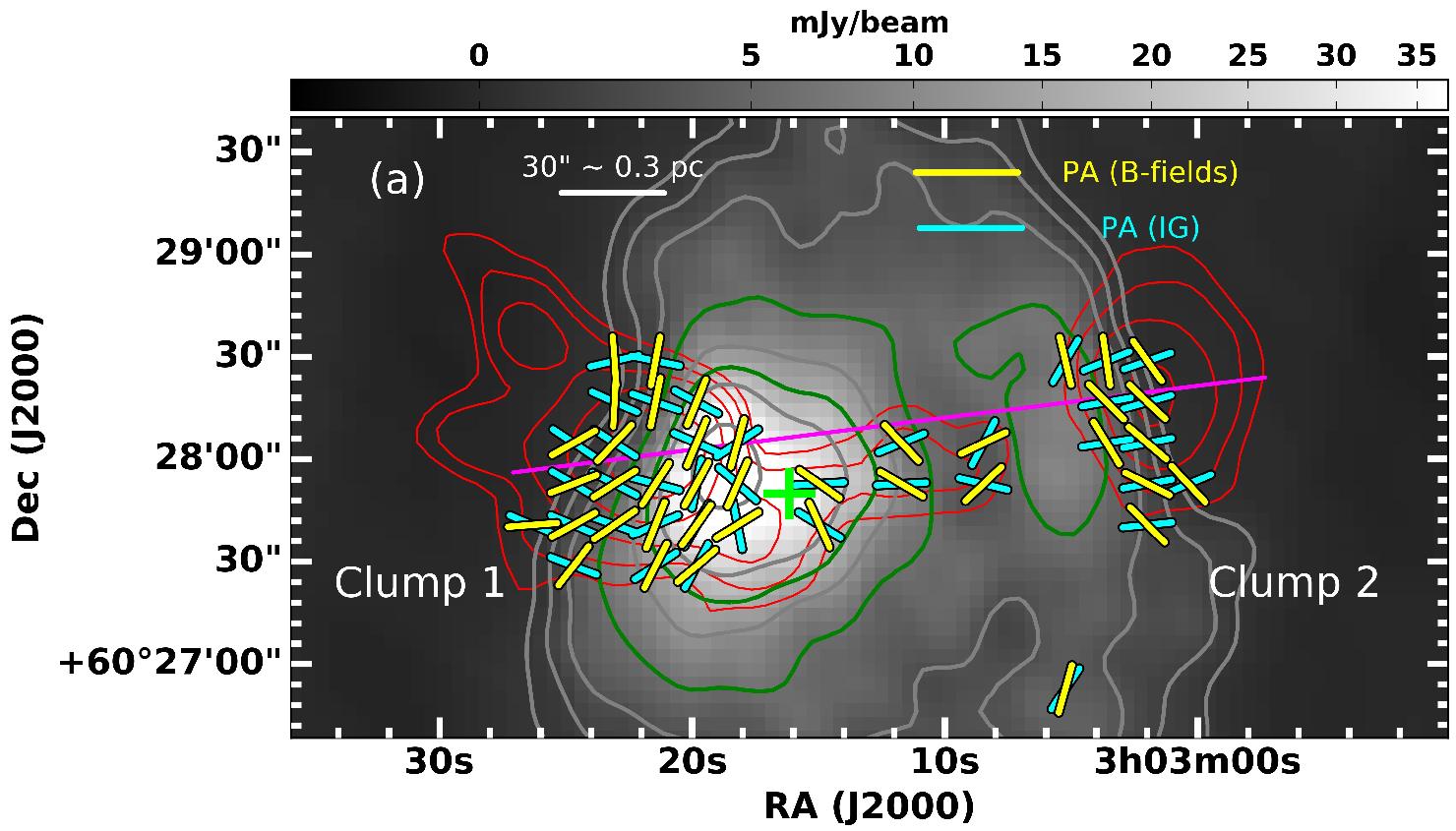
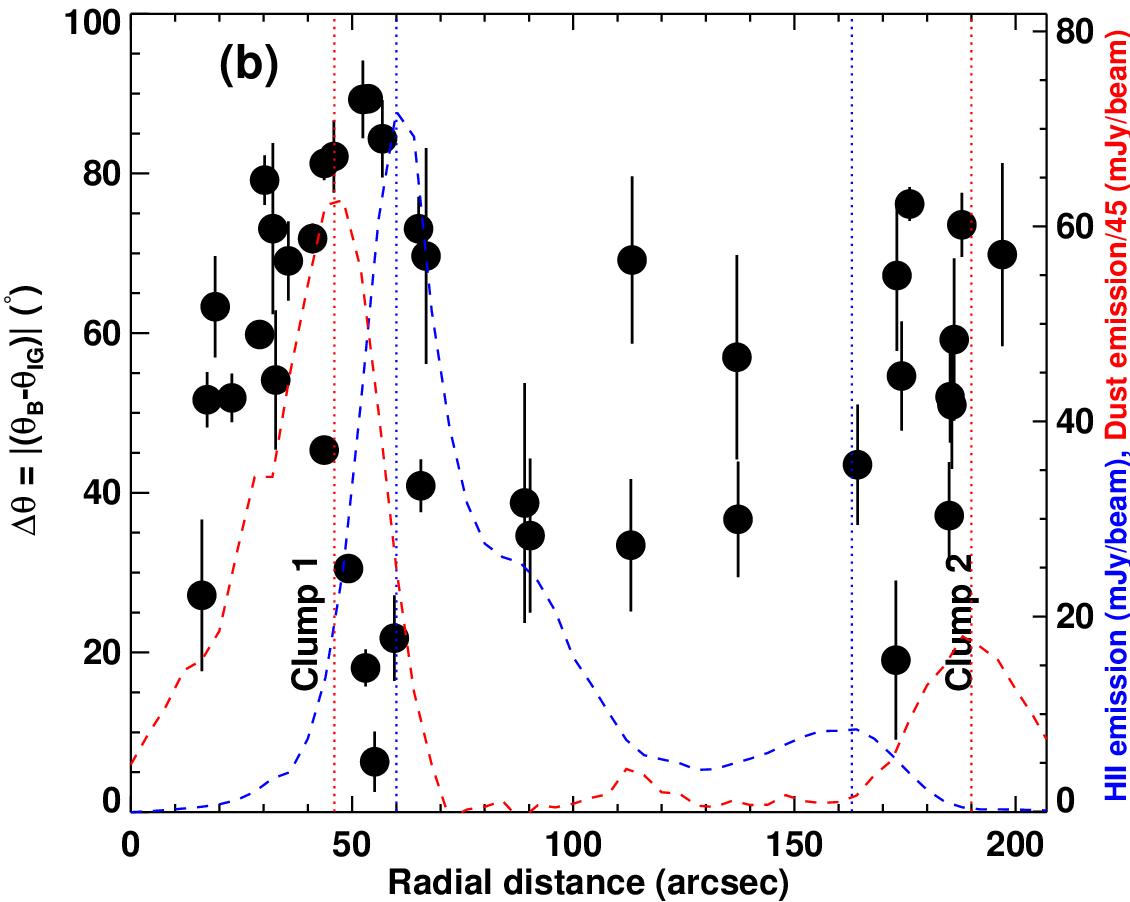
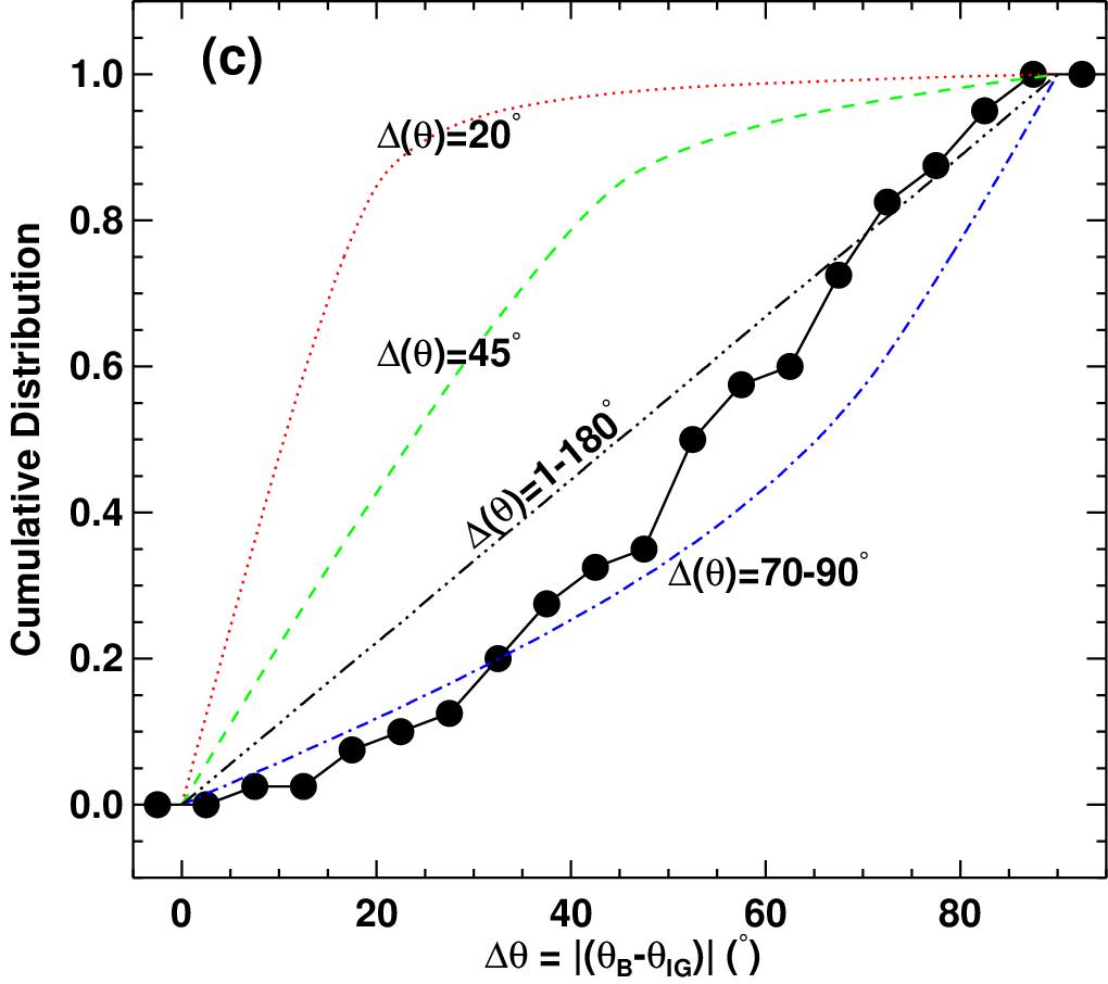
Figure 5: (a) The orientations of B-fields ($\theta_{B}$; yellow vectors) and Intensity Gradients ($\theta_{IG}$; cyan vectors) are overlaid on the VLA 1.45 GHz continuum map. Red and gray contours are the same as those shown in Figure 3. Integrated fluxes within the green contours correspond to 26$\sigma$ and 70$\sigma$ flux levels of 0.006 Jy/beam and 0.016 Jy/beam around clumps 1 and 2, respectively, are used for estimating the thermal pressures exerted on the respective clump surfaces (c.f. Section 3.6 for more details). Locations of the clumps and reference scale length are also shown. Radial profiles of dust and H ii emission are extracted along the magenta line and are drawn in panel (b). (b) The offset between the position angles of B-fields and intensity gradients, i.e., $\Delta\theta$ $=$ $|(\theta_{B}-\theta_{IG})|$ as a function of radial distance (filled circles). The zero radial distance points to the left edge of the magenta line close to the clump 1. Also, in the right-hand of y-axis, we plotted the radial variation of radio emission (VLA 21 cm; blue dashed lines) as well as of the dust emission (SCUBAPOL2 Stokes I; red dashed line) along the same magenta line shown in panel (a). (c) Cumulative distribution of $\Delta\theta$ $=$ $|(\theta_{B}-\theta_{IG})|$ is shown with filled circles. Model cumulative distributions (lines with different colors) for $\Delta\theta$ values of 20$\arcdeg$, 45$\arcdeg$, 70-90$\arcdeg$, and random angles, adopted from Monte Carlo simulations (Hull et al., 2014), are also shown.

Figure 5(b) shows the offset angle ($\Delta\theta$) between $\theta_{\mathrm{B}}$ and $\theta_{\mathrm{IG}}$ as a function of radial distance (from clump 1 to clump 2) along the magenta line shown in Figure 5(a). The radial profiles of dust and H ii emission, extracted along the magenta line, are also shown to examine their correlation with the $\Delta\theta$ values. At radial distances $<$ 70$\arcsec$ and $>$ 160$\arcsec$, where the dust and H ii emission peaks of clump 1 and 2, respectively, are found, the majority of the $\Delta\theta$’s lie between $\sim$50$\arcdeg$ and $\sim$90$\arcdeg$. Notably, perpendicular components prevail around clump 1, and also at clump 2, albeit with less prominence due to the lack of $\Delta\theta$ values in the range 70$\arcdeg$ to 90$\arcdeg$. Here, $\Delta\theta$ $=$ 90$\arcdeg$ refers to perpendicular alignment of B-fields with intensity gradients or parallel alignment of B-fields with intensity contours. Between clumps 1 and 2, i.e., from $\sim 80\arcsec$ to $\sim 150\arcsec$, the $\Delta\theta$ values are neither parallel nor perpendicular, lying between $\sim 30\arcdeg$ and $\sim 40\arcdeg$. These values contribute towards the random component as evident from Figures 5(b) and (c). In addition, there also exist a few parallel components ($\sim 0\arcdeg$ – $\sim 30\arcdeg$) near clump 1 and clump 2.

Therefore, at clump 1, because of the prominent interaction between the dust and H ii emissions, B-fields tend to be perpendicular to the intensity gradients ($\theta_{\mathrm{IG}}$) or parallel to the intensity contours. Whereas at clump 2, as the interaction between the dust and the H ii region is less prominent (based on their peak brightness in comparison to those of clump 1), a lower degree of alignment between B-fields and intensity contours is evident. The cumulative distribution of $\Delta{\theta}$ values also confirms the possibility of both perpendicular and random components, as shown in Figure 5(c). In order to study the projection effect from alignments between B-fields and intensity gradients in three-dimensional space to those in the plane of the sky, we also show cumulative distributions based on Monte Carlo simulations (Hull et al., 2014). These simulations randomly select pairs of orientations in three dimensions that have alignments in the ranges 0$\arcdeg$ – 20$\arcdeg$, 0$\arcdeg$ – 45$\arcdeg$, 70$\arcdeg$ – 90$\arcdeg$, or random alignment; then their $\Delta{\theta}$ are measured on the plane of the sky. The resulting cumulative distribution functions of the simulations are shown in Figure 5(c). Kolmogorov-Smirnov statistics suggest that, with a probability of 82.5%, our data is consistent with the model distribution corresponding to a $\Delta{\theta}$ of 70 – 90$\arcdeg$, while there is a probability of only 26.5% that our data have a random component. Therefore, we conclude that the B-fields in the clumps are shaped by the H ii region.

3.3 Dust properties of the clumps: column density, number density, and mass

For an idealized cloud, the dust emission at frequencies where optical depth is small can be described by (Hildebrand 1983; see also Li et al. 1999)

$$S(\nu)=N(\sigma/D^{2})Q(\nu)B(\nu,T_{d}),$$ (1)

where $S(\nu)$ is the flux density (erg s^-1 cm^-2 Hz^-1 or Jy) from a cloud at distance $D$, $N$ is the number of spherical grains included in the cloud volume subtended by the beam, $Q(\nu)$ is the dimensionless absorption coefficient, $\sigma$ is the geometric cross section of a dust grain, and $B(\nu,T_{d})$ is the Planck function for a blackbody at temperature $T_{d}$.

The above equation can be written as follows to construct the column density map from the POL2 850 $\mu$m Stokes I map (Kauffmann, 2007),

$$N_{\mathrm{H_{2}}}=2.02\times 10^{20}\mathrm{cm^{-2}}\left(e^{1.439{\left(\frac{\lambda}{\mathrm{mm}}\right)}^{-1}{\left(\frac{\mathrm{T_{d}}}{\mathrm{10K}}\right)}^{-1}}-1\right)$$

$${\left(\frac{\kappa_{\nu}}{0.01\,{\mathrm{cm^{2}\,g^{-1}}}}\right)}^{-1}\left(\frac{{S_{\nu}}^{\mathrm{beam}}}{\mathrm{mJy\,beam^{-1}}}\right){\left(\frac{\theta_{\mathrm{HPBW}}}{\mathrm{10\,arcsec}}\right)}^{-2}{\left(\frac{\lambda}{\mathrm{mm}}\right)}^{3},$$

where $T_{d}$ is the mean dust temperature within the two clumps, $\lambda$ $=$ 0.85 mm, and $\theta_{\mathrm{HPBW}}$ $=$ beam size (14$\arcsec$), $\kappa_{\nu}=0.1(\nu/1\mathrm{THz})^{\beta}=0.0182$ is the dust opacity in cm² g^-1, and $\beta$ is the dust opacity exponent of 2 (e.g., Arzoumanian et al. 2011).

We have performed CASA 2D Gaussian fits on the POL2 850 $\mu$m Stokes I map, specifically on the pixels around each clump having I $>$ 140 mJy/beam (i.e., $>$10$\sigma$, where $\sigma$ = 14 mJy beam^-1 is the rms noise in the I map with pixel size $=$ 4$\arcsec$), and extracted the spatial extents of the clumps. The resultant dimensions of the clumps, along with their central coordinates, are given in Table 2. The effective radius of each clump is $R_{\mathrm{eff}}$ $=$ $\sqrt{\sigma_{a}\times\sigma_{b}}$; where $\sigma_{a}$ and $\sigma_{b}$ are the extents of the semimajor and semiminor axes, respectively, and are found to be 13.3$\pm$0.3$\arcsec$ (or 0.13$\pm$0.01 pc) for clump 1 and 15.2$\pm$0.4$\arcsec$ (or 0.15$\pm$0.01 pc) for clump 2. The mean dust temperatures ($T_{d}$), within the dimensions of clump 1 and clump 2, are estimated to be 27 K and 29 K (Deharveng et al., 2012), and are used in the above Equation to estimate the respective column density maps.

The total column densities ($\sum N_{H_{2}}$) are estimated within the clump dimensions, and are found to be (9.2$\pm$1.6)$\times$10²³ cm^-2 for clump 1 and (3.5$\pm$0.5)$\times$10²³ cm^-2 for clump 2. The number density ($n(H_{2})$) is estimated using the relation

$$n(H_{2})=\frac{\sum\,N_{H_{2}}\,\times\,A_{\mathrm{pixel}}}{{\frac{4}{3}}{{\pi\,R_{\mathrm{eff}}}^{3}}},$$ (2)

where $A_{pixel}$ is the area of a pixel (4$\arcsec$) in cm². $R_{eff}$ is the effective radius (estimated above). The derived number densities for clumps 1 and 2, respectively, are (5.1$\pm$0.9)$\times$10⁴ cm^-3 and (1.3$\pm$0.2)$\times$10⁴ cm^-3. The mean column density ($N_{H_{2}}$) for clump 1 is (27$\pm$6)$\times$10²¹ cm^-2 and for clump 2 is (8$\pm$1)$\times$10²¹ cm^-2.

We have estimated clump mass using the relation

$$M~{}=~{}A_{pixel}\,\mu_{H_{2}}\,m_{H}\,\sum N_{H_{2}}.$$ (3)

Here we used the integrated total column densities, $\sum N_{H_{2}}$, within the contours corresponding to 10$\sigma$ Stokes I. The resulting masses are found to be 72$\pm$5 M_☉ and 22$\pm$2 M_☉ for clumps 1 and 2, respectively.

We note that the masses determined above are likely to be lower limits on the true masses because they have been estimated using the average dust temperature over the clump areas. We thus measured masses within the areas corresponding to 10$\sigma$ Stokes I but from the column density map constructed from the Herschel temperature map (for details see Deharveng et al. 2012). The resulting masses are found to be 191$\pm$13 M_☉ and 30$\pm$3 M_☉ for clump 1 and clump 2, respectively. Although these values agree within a factor of two with the masses derived from 850 $\mu$m Stokes I map, they are likely to better represent the true masses. We thus used these values for further analyses. The number densities and masses estimated above are listed in Table 2.

3.4 Gas properties: velocity dispersion

Figure 6 shows the JCMT HARP/ACSIS ¹³CO(3–2) and C¹⁸O(3–2) spectra of the two clumps, averaged over the clump dimensions, in units of brightness temperature ($T_{b}$, K) versus velocity (V_LSR, km s^-1). We performed Gaussian fitting on each spectrum, resultant peak brightness temperature ($T_{b,p}$), central V_LSR, and velocity dispersion ($\sigma_{V_{\mathrm{LSR}}}$) values are given in Table 3. The $\sigma_{V_{\mathrm{LSR}}}$ values for clumps 1 and 2 are 1.05$\pm$0.01 km s^-1 and 1.06$\pm$0.01 km s^-1 in ¹³CO, and 0.69$\pm$0.02 km s^-1 and 0.60$\pm$0.04 km s^-1 in C¹⁸O. For clump 1, using C¹⁸O (J=1–0) measurements, Niwa et al. (2009, clump 9 in their work) derived the mean velocity dispersion over an area somewhat larger than that we consider as 0.71 km s^-1, which is in close agreement with our estimate derived from C¹⁸O(3–2).

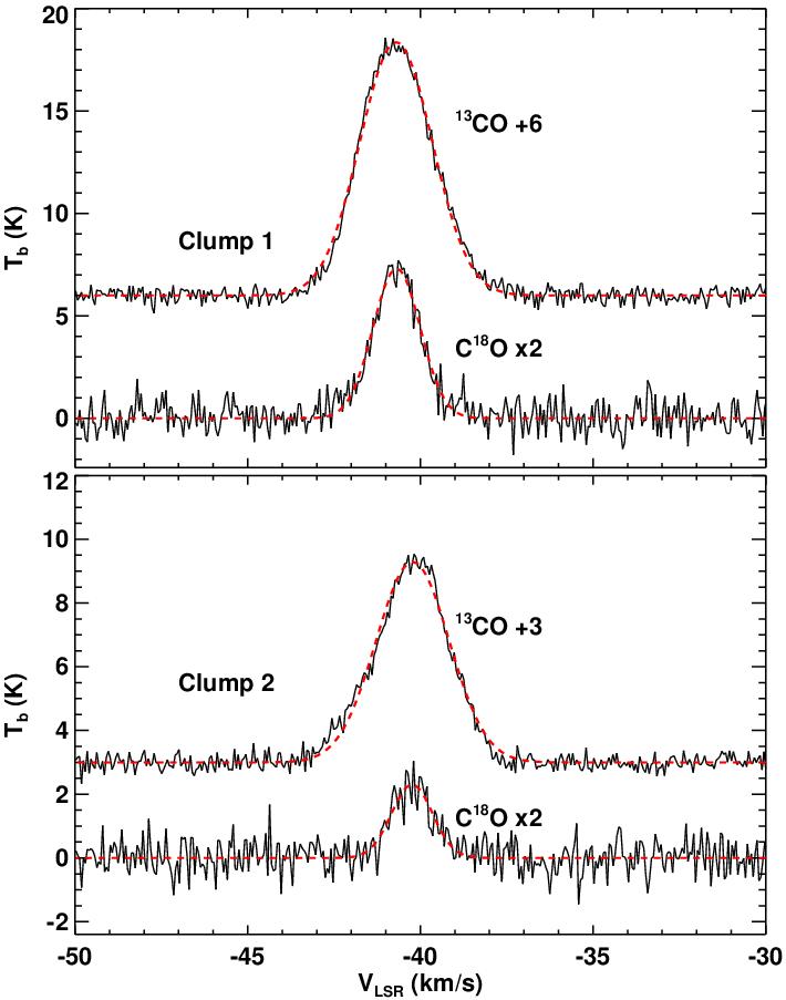
Figure 6: ¹³CO (3–2) and C¹⁸O (3–2) brightness temperature versus $V_{\mathrm{LSR}}$ spectra, averaged over the extents of clumps 1 (top) and 2 (bottom). To view clearly, the spectra of ¹³CO and C¹⁸O are shifted by adding and multiplying by arbitrary numbers as shown in the figure. Best-fit Gaussians are shown with red dashed lines.

The ¹³CO gas traces the extended low-density gas around the clumps, whereas C¹⁸O traces the highly compact central dense regions of the clumps (see Figure 7). To demonstrate this, we estimate the optical depths, column densities of ¹³CO and C¹⁸O , and the resultant $H_{2}$ column densities in Appendix B; these values are listed in Table 4. The optical depths suggest that C¹⁸O is optically thin and hence traces the densest parts of the clumps, thereby revealing the level of turbulence at the densities traced by 850 $\mu$m dust emission.

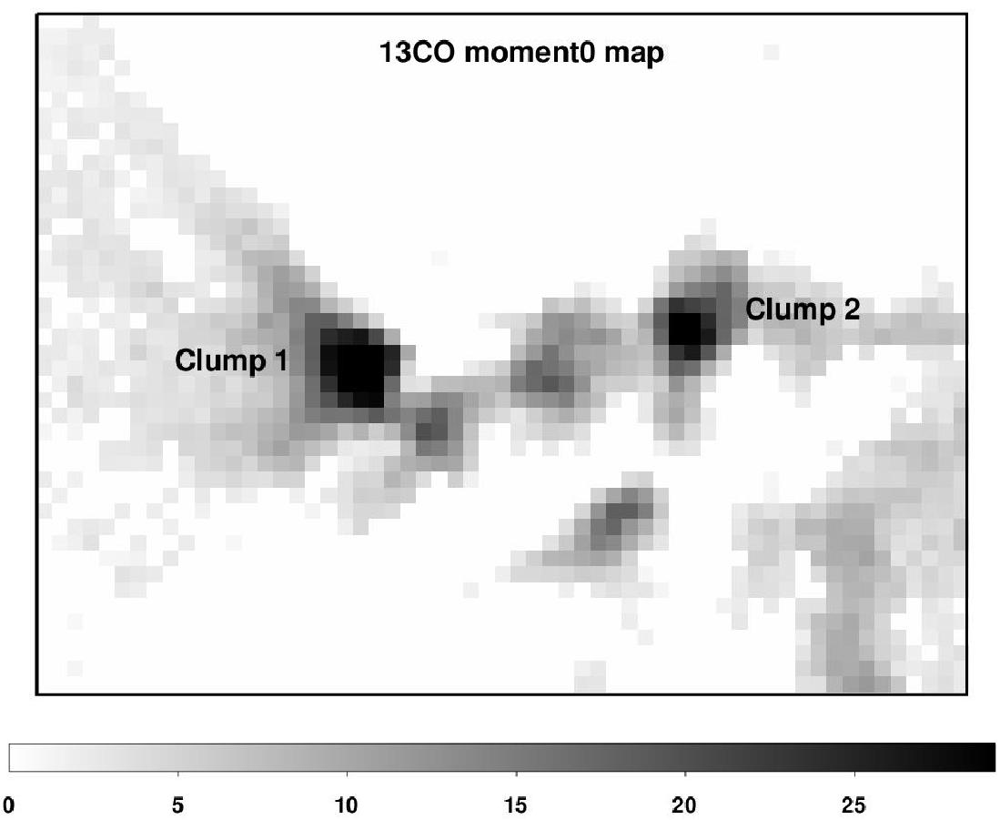
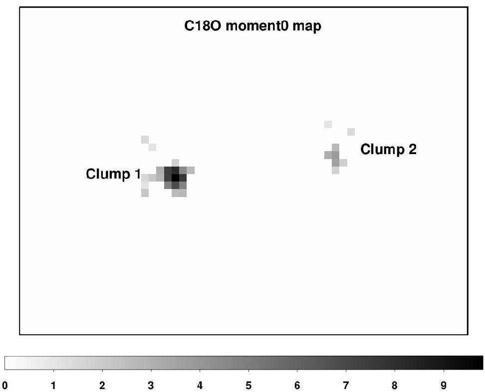
Figure 7: Velocity integrated intensity maps of the S201 region showing the two clumps (identified as clumps 1 and 2) in ¹³CO (left) and C¹⁸O (right). The color scales correspond to the velocity-integrated intensity in K km s^-1. The central coordinates of the maps are $\alpha_{J2000}$ $=$ 03^h03^m12$\fs$72, $\delta_{J2000}$ $=$ $+$60$\arcdeg$28$\arcmin$08$\farcs$01 and the dimensions are $\sim 7\arcmin\times\sim 5\arcmin$. North is up and east is to the left.

We further derive the one-dimensional thermal velocity dispersion ($\sigma_{\mathrm{T}}$) implied by the kinetic temperature of the C¹⁸O gas using the relation

$$\sigma_{T}=\sqrt{\frac{k\,T_{\mathrm{kin}}}{{M_{\mathrm{C^{18}O}}}}},$$ (4)

where $k$ is the Boltzmann constant, $T_{\mathrm{kin}}$ is gas kinetic temperature, which is equivalent to the mean dust temperatures ($T_{\mathrm{d}}$ $=$ 27 K and 29 K for clump 1 and 2; Table 2) under the assumption that the gas and dust are in local thermal equilibrium. $M_{\mathrm{C^{18}O}}$ is the mass of the C¹⁸O molecule and is considered to be 30 amu. The estimated $\sigma_{\mathrm{T}}$ values are found to be 0.087$\pm$0.024 km s^-1 and 0.090$\pm$0.017 km s^-1 for clumps 1 and 2. Finally, the non-thermal velocity dispersion ($\sigma_{\mathrm{NT}}$), which is due to the turbulence, is estimated by correcting for thermal velocity dispersion using the relation

$$\sigma_{\mathrm{NT}}=\sqrt{{\sigma_{\mathrm{V_{LSR}}}}^{2}-{\sigma_{\mathrm{T}}}^{2}}.$$ (5)

The derived $\sigma_{\mathrm{NT}}$ values are 0.68$\pm$0.02 km s^-1 and 0.59$\pm$0.04 km s^-1 for clumps 1 and 2, respectively. Therefore, in the following analysis we used our derived C¹⁸O non-thermal velocity dispersions, $\sigma_{\mathrm{NT}}$, to estimate the B-field strength and pressure, turbulent pressure, Alfvénic velocity, Alfvén Mach number, virial mass, etc.

3.5 Magnetic field strength

In the subsections above, number densities and gas velocity dispersion values were extracted. Here, we derive the angular dispersion of the B-fields in order to estimate the B-field strength and other crucial parameters.

The plane-of-sky component of B-field strength ($B_{pos}$) can be estimated using the Davis-Chandrasekhar-Fermi method (Davis, 1951; Chandrasekhar & Fermi, 1953, hereafter DCF method), which is based on the assumption that turbulence-induced Alfvén waves will distort B-field orientations. This method assumes that the following two conditions hold: (a) the ratio of turbulent (${\delta}B$) to large-scale ordered ($B_{o}$) B-field components is proportional to the ratio of one-dimensional non-thermal velocity dispersion ($\sigma_{v}$) to Alfvénic velocity ($V_{A}$ $=$ $B_{o}/\sqrt{4\pi\rho}$; where $\rho$ is the mass density), i.e., $\delta B/B_{o}\sim\sigma_{v}/V_{A}$ (Hildebrand et al., 2009), and (b) ${\delta}B/B_{o}\sim\sigma_{\theta}$, where $\sigma_{\theta}$ is the dispersion in the measured B-field orientation. The DCF method can be applied to sets of Gaussian-distributed polarization angles with angular dispersions less than 25$\arcdeg$ (Ostriker et al., 2001). However, B-fields in regions altered by H ii regions or dragged by gravity will generally exhibit multiple components, and so have a significantly higher angular dispersions (e.g., Arthur et al., 2011; Chapman et al., 2011; Santos et al., 2014; Eswaraiah et al., 2017; Chen et al., 2017). As shown in Figure 4, the histograms of B-fields being impacted by the H ii region feedback exhibit either a widely spread distribution of angles or multiple distributions with conspicuously separate peaks. In such regions alternative methods must be employed to extract the underlying dispersion in polarization angles caused by magnetized turbulence. Progress has recently been made towards the accurate estimation of ${\delta}B/B_{o}$ through statistical analyses of polarization angles. These analyses include the “structure function" (Hildebrand et al., 2009) and the “auto-correlation function" (Houde et al., 2009) of polarization angles. These are referred to as modified DCF methods, and used to estimate the B-fields in such regions.

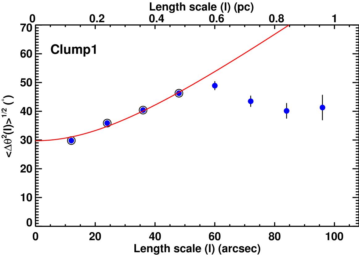
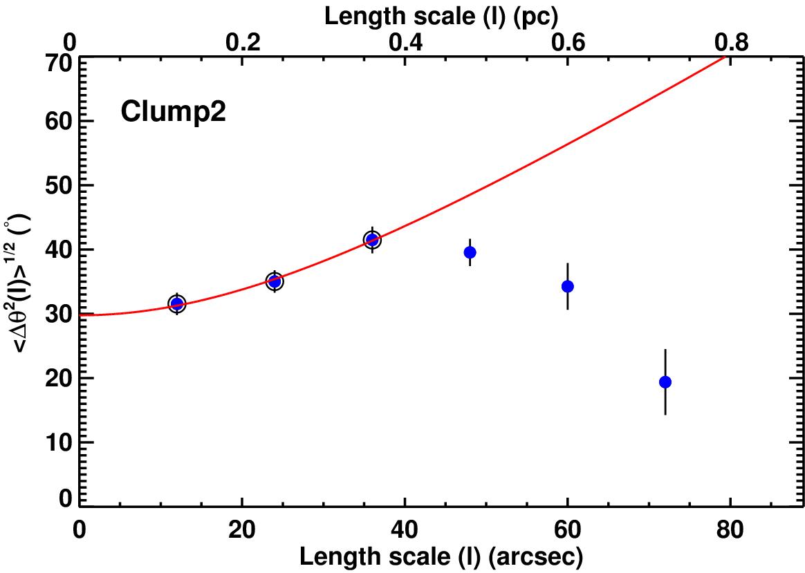
Figure 8: Angular dispersion function versus length scale for clump 1 (left) and clump 2 (right). The plotted angular dispersions (blue filled circles) are corrected for measured uncertainties. The best fits are shown with red lines. The data considered for the fits are depicted with encircled symbols.

3.5.1 Structure function (SF) analysis

In the structure function (SF) analysis (Hildebrand et al., 2009), the B-field is assumed to consist of a large-scale structured field, $B_{o}$, and a turbulent component, ${\delta}B$. The SF analysis demonstrates the variation of dispersion in position angles as a function of vector separation $l$. At some scale larger than the turbulent scale $\delta$, ${\delta}B$ should reach its maximum value. At scales smaller than a scale $d$, the higher-order terms of the Taylor expansion of $B_{0}$ can be canceled out. When $\delta<l\ll d$, the SF follows the form:

$$\langle\Delta\Phi^{2}(l)\rangle_{\mathrm{tot}}-\sigma_{M}^{2}(l)\simeq b^{2}+m^{2}l^{2}.$$ (6)

In this equation, $\langle\Delta\Phi^{2}(l)\rangle_{\mathrm{tot}}$, the square of the total measured dispersion function, consists of $b^{2}$, a constant turbulent contribution, $m^{2}l^{2}$, the contribution from the large-scale structured field, and $\sigma_{M}^{2}(l)$, the contribution of the measured uncertainty. The ratio of the turbulent to the large-scale component of the magnetic field is given by:

$$\frac{\langle{\delta}B^{2}\rangle^{1/2}}{B_{o}}=\frac{b}{\sqrt{2-b^{2}}}.$$ (7)

And $B_{o}$ is estimated using the modified DCF relation:

$$B_{o}\simeq\sqrt{(2-b^{2})4\pi\mu m_{\mathrm{H}}n_{\mathrm{H_{2}}}}\frac{\sigma_{v}}{b}.$$ (8)

Then the estimated plane-of-sky magnetic field strength is corrected by a factor $Q$

$$B_{\mathrm{pos}}=Q~{}B_{0}$$ (9)

where $Q$ is considered as 0.5 based on studies using synthetic polarization maps generated from numerically simulated clouds (Ostriker et al., 2001), which suggest that B-field strength is uncertain by a factor of two when the B-field dispersion is $\leq$ 25$\arcdeg$.

The blue filled circles plotted in Figure 8 represent the angular dispersions corrected for uncertainties ($\langle\Delta\Phi^{2}(l)\rangle_{\mathrm{tot}}-\sigma_{M}^{2}(l)$) as a function of length scale, measured from the polarization data. The bin size of 12$\arcsec$, used in Figure 8, corresponds to the grid size of the polarization catalog yielded by pol2map. The maximum value in the current SF is lower than the value expected for a random field (52$\arcdeg$, Poidevin et al., 2010). Equation 6 is fitted to the data using the IDL MPFIT nonlinear least-squares fitting algorithm (Markwardt, 2009). The resulting $\frac{\langle{\delta}B^{2}\rangle^{1/2}}{B_{o}}$ values are 0.40$\pm$0.02 and 0.40$\pm$0.07 for clumps 1 and 2, and the corresponding $B_{pos}$ strengths are derived using equations 7, 8, and 9 to be 147$\pm$15 $\mu$G and 65$\pm$6 $\mu$G.

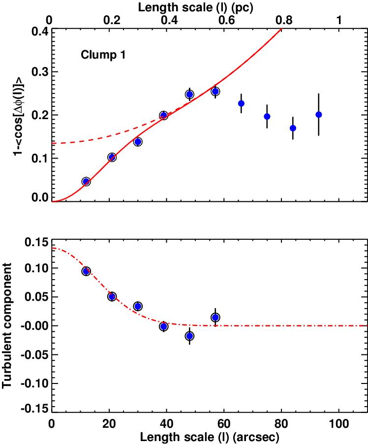
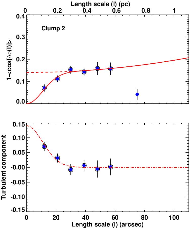
Figure 9: (Top) Auto-correlation function versus length scale for clump 1 (left) and clump 2 (right). Angular dispersions are shown as filled circles. The red continuous line shows the best fit dispersion function and the red dashed line shows the large-scale ordered or non-correlated components (1/N) ($\left<\delta B^{2}\right>/\left<B_{o}^{2}\right>$) + $a_{2}^{{}^{\prime}}l^{2}$. The data used in the fits are depicted with encircled filled symbols. (Bottom) Best fit turbulent or correlated component (1/N) ($\left<\delta B^{2}\right>/\left<B_{o}^{2}\right>$) $e^{-l^{2}/2(\delta^{2}+2W^{2})}$ for clump 1 and clump 2, shown with dot-dashed lines. Plotted data points correspond to the difference between the derived angular dispersions (encircled filled symbols; top panels) and the large-scale ordered component (red dashed line; top panels).

3.5.2 Auto-correlation function (ACF) analysis

Auto-correlation function (ACF) analysis (Houde et al., 2009) is an extension of SF analysis, which includes the effect of signal integration along the line of sight as well as within the beam. According to Houde et al. (2009), the ACF can be written as:

$$1-\langle\cos[\Delta\Phi(l)]\rangle\simeq\frac{1}{N}\frac{\langle{\delta}B^{2}\rangle}{\langle B_{0}^{2}\rangle}\times[1-e^{-l^{2}/2(\delta^{2}+2W^{2})}]+a_{2}\arcmin l^{2},$$ (10)

where $\Delta\Phi(l)$ is the difference in position angle of two vectors separated by a distance $l$, $W$ is the beam radius (6.0$\arcsec$ for the JCMT, i.e., the FWHM beam size of 14$\arcsec$ divided by $\sqrt{8\ln{2}}$), $a_{2}\arcmin$ is the slope of the second-order term of the Taylor expansion, and $\delta$ is the turbulent correlation length. $N$ is the number of turbulent cells probed by the telescope beam and is given by:

$$N=\frac{(\delta^{2}+2W^{2})\Delta\arcmin}{\sqrt{2\pi}\delta^{3}},$$ (11)

where $\Delta\arcmin$ is the effective thickness of the cloud. The ordered magnetic field strength is given by

$$B_{o}\simeq\sqrt{4\pi\mu m_{\mathrm{H}}n_{\mathrm{H_{2}}}}\sigma_{v}\left[\frac{\langle{\delta}B^{2}\rangle}{\langle B_{o}^{2}\rangle}\right]^{-1/2}.$$ (12)

The top panels of Figure 9 show the angular dispersion functions of the polarization vectors in clumps 1 and 2, while the bottom panels show the respective correlated components of the dispersion functions. In our fitting, $\Delta\arcmin$ is set to $31\arcsec\pm 1\arcsec$ for clump 1 and $36\arcsec\pm 1\arcsec$ for clump 2 (these correspond to the effective thickness of the clumps, derived using the relation $\sqrt{\delta_{a}\times\delta_{b}}$; where $\delta_{a}$ and $\delta_{b}$ are the FWHMs of the major and minor axes, respectively (see Table 2).

Equation 10 is fitted to the ACF data shown in Figure 9 for clumps 1 (top panel) and 2 (bottom panel). The bin width for constructing the ACF ($1-\langle\cos[\Delta\Phi(l)]\rangle$) function was chosen to be 9$\arcsec$. Various bin widths were investigated; we found that best fit was achieved with a bin width of 9$\arcsec$. The IDL MPFIT non-linear least-square fitting algorithm (Markwardt, 2009) was used and simultaneously constrained the three fitting parameters (i) $\delta$, (ii) $\frac{\langle{\delta}B^{2}\rangle}{\langle B_{o}^{2}\rangle}$, and (iii) ${a_{2}}\arcmin$; the best-fit values are listed in Table 2. Using the fitted parameter $\frac{\langle{\delta}B^{2}\rangle}{\langle B_{o}^{2}\rangle}$, along with derived parameters such as number densities and velocity dispersions, we have estimated the B-field strength using the modified DCF relation (equation 12). The estimated B-field strengths are 266$\pm$32 $\mu$G and 61$\pm$31 $\mu$G for clumps 1 and 2 respectively. The turbulent correlation length $\delta$ is $13\pm 3\arcsec$ (126$\pm$29 mpc) and $7\pm 4\arcsec$ (68$\pm$36 mpc) for clumps 1 and 2. The number of turbulent cells (N) is derived to be 1.4$\pm$0.4 and 5.0$\pm$4.8 for clumps 1 and 2, respectively. The derived parameters are listed in Table 2.

In summary, the SF and ACF analyses yielded two B-field strengths: for clump 1 these differ by a factor of $\sim$2 (147$\pm$15 $\mu$G and 266$\pm$32 $\mu$G), while they are nearly identical for clump 2 (65$\pm$6 $\mu$G and 61$\pm$31 $\mu$G), although the ACF-derived B-field strength has $\sim$50% uncertainty. It should be noted here that the measured uncertainties in the B-fields strengths are 15 $\mu$G and 32 $\mu$G for clump 1 and 6 $\mu$G and 31 $\mu$G for clump 2. These are random errors, resulting from propagation of the uncertainties of various parameters (such as gas number density, gas velocity dispersion, and B-field angular dispersion) through the modified DCF formulae. We caution here that, in practice these measurement errors can be dominated by systematic errors associated with various parameters such as dust opacity, dust temperature, flux calibration, clump geometry (and hence depth), and inclination angle, etc. (e.g., Pattle et al., 2017; Wang et al., 2019; Liu et al., 2019). These factors could be more severe in clump 1 because of the existence of more extended emission around the peak of dust emission. Therefore the real uncertainties could be much larger than the quoted errors in B-field strengths.

It is clear from Sections 3.5.2 and 3.5.1 above (see also Table 2) that for clump 2 the ACF-yielded parameters have higher uncertainties in comparison to those yielded by SF. This could be attributed to the relatively small number of vectors in clump 2 causing ACF to fail constraining all the fitting parameters simultaneously (see column 3 of Table 2 for ACF). In addition, since the column density is relatively lower, the beam dilution and signal integration effects may not be important in clump 2. Conversely, for clump 1 these factors seem to be crucial and taken care of ACF. Therefore, we have used B-field strengths derived from ACF (266$\pm$32 $\mu$G) for clump 1 and from SF (65$\pm$6 $\mu$G) for clump 2 in the further analyses.

3.6 Ionized gas properties: thermal and radiation pressure in S201

Figure 10 shows the radio continuum view of the S201 H ii region at VLA 21 cm/1.4 GHz. The flux density (S_ν) of S201, estimated by integrating over 3$\sigma$ contours, is $\sim$1.0$\pm$0.1 Jy, where $\sigma$ is the rms noise of the 21 cm map. Our 21 cm flux density is, within uncertainty, consistent with flux density at 6 cm (1.2$\pm$0.2 Jy; Felli et al. 1987, and references therein). The flux densities at 21 cm and 6 cm reflect a flat spectrum, indicating that the nebula is optically thin at 21 cm. Considering 8302 K as the electron temperature ($T_{\mathrm{e}}$; Balser et al. 2011) and $\sim$120$\arcsec$ (or 1.2 pc at 2 kpc) as the effective radius of the ionized gas (Figure 10), we estimated the average electron density ($n_{e}$) of the S201 H ii region using the following equations (Martín-Hernández et al., 2005)

$$n_{e}=\frac{4.092\times 10^{5}\mathrm{cm}^{-3}}{\sqrt{b(\nu,T_{e})}}\left(\frac{S_{\nu}}{\mathrm{Jy}}\right)^{0.5}\left(\frac{T_{e}}{10^{4}\mathrm{K}}\right)^{0.25}\left(\frac{D}{\mathrm{kpc}}\right)^{-0.5}\left(\frac{\theta_{D}}{\arcsec}\right)^{-1.5}$$ (13)

and

$$b(\nu,T_{e})=1+0.3195\log\left(\frac{T_{e}}{10^{4}\mathrm{K}}\right)-0.2130\log\left(\frac{\nu}{\mathrm{GHz}}\right),$$ (14)

where $S_{\nu}$ is the radio continuum integrated flux at frequency $\nu$, $\theta_{D}$ is the angular diameter of the source, $D$ (2 kpc) is the distance from the Sun, and $T_{e}$ is the electron temperature in the ionized plasma. Using this formalism, we estimated $n_{e}$ as 226$\pm$11 cm^-3. We then estimated the corresponding thermal pressure, due to ionized gas distributed over the area of diameter $\sim$120$\arcsec$, to be (5.2$\pm$0.3) $\times$ 10^-10 dyn cm^-2 using the relation $P_{\mathrm{te}}=2n_{e}k_{b}T_{e}$.

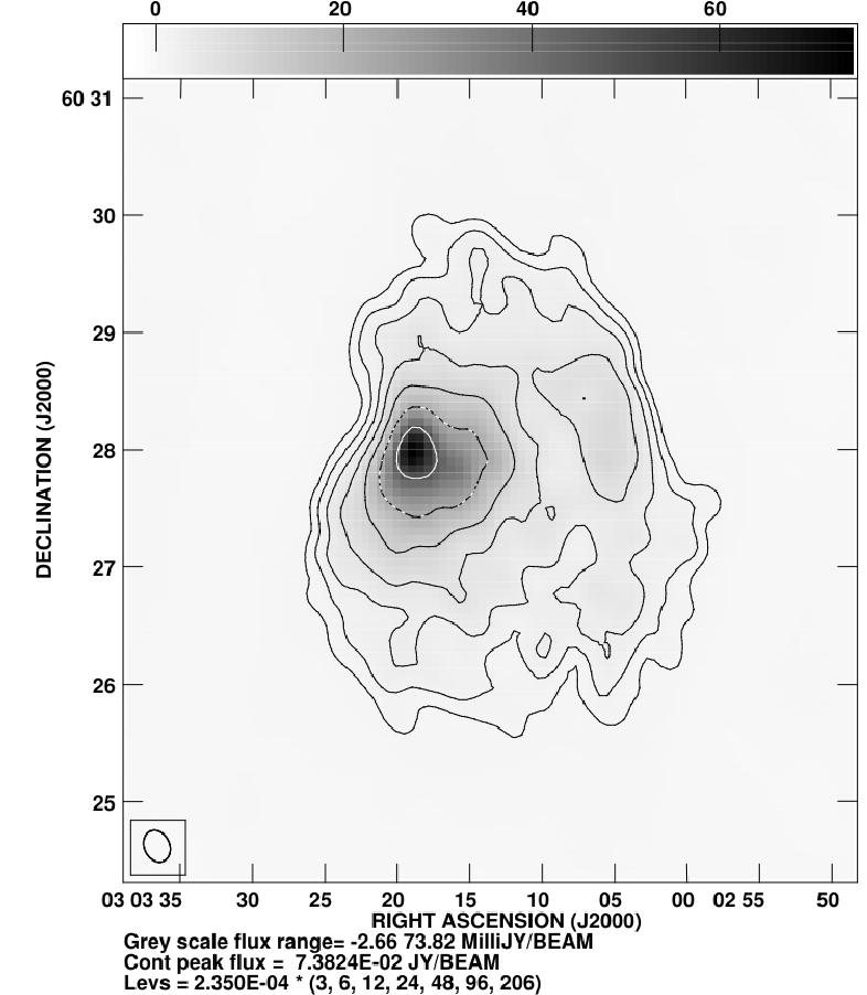
Figure 10: A radio continuum map of S201 at 1.4 GHz. The contour levels are at $[$3, 6, 12, 23, 48, 96, and 202$]$ $\times$ 2.3$\times$10^-4 Jy/beam, where 2.3$\times$10^-4 Jy/beam  is the rms noise of the map. The VLA beam size is shown in the lower-left corner of the figure, and is $\sim 17\arcsec\times\sim 13\arcsec$.

The mean thermal pressure given above my be valid for the entire region surrounded by the H ii emission. The radio emission is observed to be uneven in the region of S201 (cf. Figure 10 and also see Figure 5) in the sense that more H ii emission is concentrated close to clump 1 than is concentrated near clump 2. Because of this, the relative impact of H ii emissions, in terms of the thermal pressures acting on the clump surfaces, will be different. Therefore, we estimate average thermal pressures close to the clumps. The integrated fluxes, $S_{\nu}$, within the green contours (see Figure 5) extended over circular diameters of $\sim$66$\arcsec$ and $\sim$48$\arcsec$, are found to be 0.4$\pm$0.2 Jy and 0.05$\pm$0.01 Jy for clumps 1 and 2, respectively. Using these parameters, along with the value of  $T_{e}$ quoted above, we estimated the electron densities, $n_{e}$, as 360$\pm$80 cm^-3 and 207$\pm$14 cm^-3, and the resultant thermal pressures, $P_{te}$, to be (8$\pm$2) $\times$ 10^-10 dyn cm^-2 and (4.7$\pm$0.3) $\times$ 10^-10 dyn cm^-2 for clumps 1 and 2, respectively.

We estimated the mean radiation pressure ($P_{rad}$) driven by an ionizing star of spectral type O6V (Ojha et al., 2004; Deharveng et al., 2012). The ionizing flux emitted by one O6V star is $q_{0}$ $=$ 4.15$\times 10^{10}$ photons cm^-2 s^-1 (Sternberg et al., 2003), and each UV photon carries an energy h$\nu$ $=$ 20 eV, so the estimated $P_{rad}$, using the relation $P_{rad}$ $=$ $h\nu~{}q_{0}/c$, is $0.44\times 10^{-10}$ dyn cm^-2. We note here that the same $P_{rad}$ value is used for both clumps and in both cases is negligible in comparison to the thermal pressures. The derived thermal and radiation pressure values are listed in Table 2.

4 Discussion

Here we discuss the interplay amongst various key parameters, clump stability based on virial and critical mass estimations, and their relevance to the formation and evolution of clumps as well as to the feedback process.

4.1 B-fields versus Turbulence

For clump 1 the magnetic and turbulent pressures, estimated using the relations $P_{B}$ $=$ $B^{2}/8\pi$ and $P_{\mathrm{turb}}$ $=$ $\rho{\sigma_{\mathrm{NT}}}^{2}$ (c.f. Section 3.4), are found to be (28 $\pm$ 7)$\times$10^-10 dyn cm^-2 and (11 $\pm$ 2)$\times$10^-10 dyn cm^-2, respectively. Similarly, for clump 2, these values are found to be (1.7 $\pm$ 0.3)$\times$10^-10 dyn cm^-2 and (2.1 $\pm$ 0.4)$\times$10^-10 dyn cm^-2. The magnetic to turbulent pressure ratios, $P_{\mathrm{B}}$/$P_{\mathrm{turb}}$, are estimated to be 2.6 $\pm$ 0.8 and 0.8 $\pm$ 0.2 for clump 1 and 2, respectively. This suggests that B-fields dominate over turbulence in clump 1, whereas turbulence dominates over B-fields in clump 2.

The turbulent Alfvén Mach number ($M_{A}$) describes the relative importance of B-fields compared to that of turbulence, and hence it is a key parameter in models of cloud formation and evolution (e.g., Ostriker et al., 2001; Padoan et al., 2001; Nakamura & Li, 2008). In the sub-Alfvénic case ($M_{A}\leqslant$ 1), B-fields are strong enough to regulate turbulence, causing an organized B-field orientation. In the super-Alfvénic case ($M_{A}>$ 1), the turbulence is capable of perturbing the morphology of B-fields.

The Alfvénic velocity, $V_{\mathrm{A}}$ $=$ $\frac{B_{\mathrm{los}}}{\sqrt{4\pi\,\rho}}$ (where $\rho$ $=$ $n_{H_{\mathrm{2}}}\,\mu\,m_{\mathrm{H}}$), is estimated to be 1.6$\pm$0.2 km s^-1 for clump 1 and 0.7$\pm$0.1 km s^-1 for clump 2. The Alfvén Mach number, $M_{\mathrm{A}}$ $=$ $\sqrt{3}(\frac{\sigma_{\mathrm{NT}}}{V_{\mathrm{A}}})$, is estimated to be 0.8$\pm$0.1 for clump 1 and 1.4$\pm$0.2 for clump 2. These estimates agree with the findings above based on the ratios of $P_{\mathrm{B}}$/$P_{\mathrm{turb}}$, and imply that turbulent motions are sub-Alfvénic and super-Alfvénic in clumps 1 and 2, respectively.

4.2 B-field versus Thermal pressure by H ii region

The ratio of magnetic (c.f. Section 4.1) to thermal pressures (c.f. Section 3.6), P_B/P_te, is found to be 3$\pm$1 and 0.4$\pm$0.1 in clumps 1 and 2, respectively. These results imply two contrasting scenarios, in that B-fields dominate over thermal pressure acting on clump 1, whereas thermal pressure dominates over B-fields in clump 2. Evidently, B-fields are strong enough to control the expanding I-front in clump 1 and, conversely, the I-front is strong enough to dictate the B-fields in clump 2. The consequences of this interplay between B-fields and thermal pressures will be discussed in Section 4.6.

4.3 Clump stability: virial and critical mass ratios

4.3.1 Are the clumps gravitationally bound?

Considering the case in which clumps are not supported by B-fields and also not confined by external pressure (in the form of envelope material around the clumps), we estimate the viral masses and virial mass ratios.

In order for self-gravitating clumps to be in virial equilibrium, the following relation between gravitational potential energy ($|{\mathcal{G}}|$) and internal kinetic energy (${\mathcal{E}}$) should hold (McKee & Zweibel, 1992)

$${\mathcal{G}}=2{\mathcal{E}},$$ (15)

where ${\mathcal{E}}$ $=$ 3/2 M$\sigma^{2}$.

The gravitational potential energy can be written as

$${\mathcal{G}}=-\frac{3}{5}\alpha\beta\frac{GM^{2}}{r},$$ (16)

where $r$ $=$ $R_{\mathrm{eff}}$ and $G$ is the gravitational constant. $\alpha$ corresponds to a geometric factor, a function of eccentricity, and $\beta$ is a function of the power-law index of the density profile ($\rho$ $\propto$ r^-a, where $a$ $=$ 1.6 for an isothermal cloud in equilibrium; Bonnor 1956). More details on deriving these factors, assuming that the clumps are prolate ellipsoids, can be found in Li et al. (2013a, and references therein). For our given values of $\sigma$ and $r$, using the above equations, the virial mass ($M_{vir}$) can be estimated using the relation

$$M_{vir}=\frac{5}{\alpha\beta}\frac{\sigma^{2}r}{G}.$$ (17)

Taking $\sigma$ $=$ $\sigma_{\mathrm{V_{LSR}}}$ of C¹⁸O and $r$ $=$ $R_{\mathrm{eff}}$, $M_{vir}$ is estimated to be 50 $M_{\sun}$ and 40 $M_{\sun}$ for clump 1 and clump 2, respectively. For our estimated masses ($M$; 191 $M_{\sun}$ for clump 1 and 30 $M_{\sun}$ for clump 2; c.f. Section 3.3), the derived virial mass ratios, $R_{\mathrm{vir}}$ $=$ $M$/$M_{\mathrm{vir}}$ are 3.9 and 0.7 for clumps 1 and 2. Therefore, clump 1 is bound by gravity and may collapse once it becomes unstable, whereas clump 2 is gravitationally unbound.

4.3.2 Stability and Critical Mass based on Turbulence, Temperature, and B-fields

Critical mass $M_{C}$ is the maximum mass that can be supported by the combined contributions of internal velocity dispersion (contribution from turbulence and neutral gas temperature, i.e., non-thermal and thermal contributions) and B-field in the clump. The two effects can be represented as

$$M_{C}=M_{J}+M_{\mathrm{\phi}},$$ (18)

which is accurate within 5% to results from more rigorous calculations (McKee, 1989).

The Jean mass for a non-magnetic isothermal cloud (Bonnor, 1956; McKee & Zweibel, 1992) is

$$M_{J}=1.182\frac{{C_{\mathrm{eff}}}^{4}}{G^{3/2}{P_{\mathrm{env}}}^{1/2}},$$ (19)

where $C_{\mathrm{eff}}$ $=$ $\sqrt{{C_{\mathrm{s}}}^{2}+{\sigma_{\mathrm{NT}}}^{2}}$. The thermal sound speed $C_{\mathrm{s}}$ $=$ $\sqrt{\frac{k\,T_{\mathrm{kin}}}{\mu_{\mathrm{H}}\,m_{\mathrm{H}}}}$ was estimated to be 0.28$\pm$0.01 km s^-1 for clump 1 and 0.29$\pm$0.01 km s^-1 for clump 2. In this equation, $T_{\mathrm{kin}}$ = $T_{\mathrm{dust}}$ and is 27 K for clump 1 and 29 K for clump 2. The $C_{\mathrm{eff}}$ values are estimated as 0.74$\pm$0.02 km s^-1 and 0.66$\pm$0.04 km s^-1 for clumps 1 and 2.

In Equation 19, the envelope pressure (or external pressure) caused by the low-density ¹³CO gas can be estimated as

$$P_{\mathrm{env}}=n_{\mathrm{env}}\,\mu\,m_{\mathrm{H}}\,{\sigma_{\mathrm{env}}}^{2},$$ (20)

where $\sigma_{\mathrm{env}}$ is the velocity dispersion in the low-density envelope, which we treated as $\sigma_{\mathrm{env}}$ $=$ $\sigma_{\mathrm{V_{LSR}}}$ of the ¹³CO gas (c.f. Table 3), and the corresponding mean gas number densities $n_{\mathrm{env}}$ were estimated over larger extents to be $\sim$0.9$\times$10⁴ cm^-3 and $\sim$0.5$\times$10⁴ cm^-3 for clumps 1 and 2.

The maximum mass that can be supported by B-fields will be

$$M_{\mathrm{\phi}}=c_{\mathrm{\phi}}\frac{\pi Br^{2}}{G^{1/2}},$$ (21)

where $c_{\mathrm{\phi}}\sim 0.12$ according to numerical simulations (Tomisaka et al., 1988).

The estimated critical masses $M_{C}$ are 78 $M_{\sun}$ and 48 $M_{\sun}$ for clumps 1 and 2. The critical mass ratios $R_{C}$ $=$ $M/M_{C}$ are found to be 2.5 and 0.6 for clumps 1 and 2. These results suggest that for clump 1 the support rendered by the combined contributions from thermal gas energy, turbulence, and B-fields is not sufficient to counteract gravity, whereas the opposite situation prevails in clump 2, such that its stability is determined by thermal energy, turbulence, and B-fields rather than by self-gravity. This picture is further corroborated by the presence of a larger number of Class 0 and I source in and around clump 1. In contrast, clump 2 is inactive as there exist no YSOs at its center, except for a few Class I sources formed at its boundary (see Figure 2).

4.4 Compressed B-fields and enhanced B-field strength in the clumps

The B-field strength in clump 1 (266$\pm$32 $\mu$G) is larger by a factor of $\sim$4 than that in clump 2 (65$\pm$6 $\mu$G). Additionally, the spread in ADF values ($\sim$30 – $\sim 50\arcdeg$; Figure 8) as well as ACF values ($\sim$0.05 – $\sim$0.37; top panels of Figure 9) for clump 1 are relatively higher than those of clump 2 (ADF range $\sim$30 – $\sim$40$\arcdeg$; while ACF range $\sim$0.03 – $\sim$0.16). Furthermore, the spread in the offset angles ($\Delta(\theta)$) between B-fields ($\theta_{B}$) and intensity gradients ($\theta_{IG}$) in clump 1 is relatively larger than that of clump 2. These signatures imply that B-fields are more curved and draped around clump 1, thereby following a bow-like structure (see Figure 3). Similar features have been seen in clump 2, but with a lesser degree of curvature. Alūzas et al. (2014), based on 2D MHD simulations, show that when an oblique shock interacts with an isolated cylindrical cloud, the B-fields wrap around the cloud, attaining a roughly circular shape (see their Fig. 1b) similar to the B-field morphologies observed in clump 1 (Figure 3). Based on 3D radiation-magnetohydrodynamic (RMHD) simulations of pillars and globules, Mackey & Lim (2011); Mackey (2012); Mackey & Lim (2013) have shown that in the case of initially strong B-fields (160 $\mu$G) oriented perpendicular to an I-front, field lines at the head of a cometary globule get compressed into a curved morphology, by closely following the bright rim in a similar manner to our present observations towards clumps 1 and 2 (see Figure 3). These findings are consistent with other observations and MHD simulations (e.g., Lyutikov, 2006; Dursi & Pfrommer, 2008; Pfrommer & Jonathan Dursi, 2010; Arthur et al., 2011; Santos et al., 2014; Kusune et al., 2015; Klassen et al., 2017).

As can be seen from Figure 5(a), contours of dust and ionized emission are closely spaced in their zone of interaction, suggesting possible compression in the interface between the hot and cold media. This interaction has also compressed B-fields and enhanced their strength. Consequently, the stronger B-fields may shield the clumps from the H ii region. In the perpendicular field case, the B-fields get amplified directly upstream of the cloud where the flow stagnates against it, where B-field pressure and field tension continue to build (Alūzas et al., 2014, see their Fig. 1c). In MHD simulations, when B-fields get compressed their strengths become enhanced in the shells or clumps by a factor of about 5 to 6 compared to those inside the expanding H ii regions (e.g., Mac Low et al., 1994; Gregori et al., 1999; Klassen et al., 2017, see also Wareing et al. 2017 for a similar enhancement of B-field strength in environments with mechanical stellar feedback). Therefore, our results provide evidence for enhanced B-field strengths in clumps, which we attribute to the effect of thermal pressure. This is because the more the Hii region interacts with the cloud, the more the field lines are compressed, resulting in a considerable enhancement in B-field strengths.

Higher values of B-field strength around $\sim$50 – $\sim$400 $\mu$G, have been measured at the edges of H ii regions using HI/OH Zeeman measurements (Troland et al., 1986, 2016; Mayo & Troland, 2012) as well as dust extinction (e.g., Kusune et al., 2015; Eswaraiah et al., 2017; Chen et al., 2017), and emission polarization (e.g., Vallée & Fiege, 2005; Pattle et al., 2018). For example, Mayo & Troland (2012) have measured B-field strength of $\sim$80 $\mu$G using the HI Zeeman effect in the photodissociation region (PDR) DR 22, which they interpret as resulting from B-fields amplified by compression of the PDR due to absorption of the momentum of stellar radiation (also see Pellegrini et al. 2007, for a similar explanation). Based on NIR polarimetry towards the bright-rimmed cloud SFO 74, Kusune et al. (2015) have measured an enhanced B-field strength of $\sim$90 $\mu$G inside the tip rim due to UV-radiation-induced shock. Similarly, enhanced B-field strengths of 100 – 300 $\mu$G have been inferred in PDRs around ionized regions using radio recombination lines (RRLs; Balser et al. 2016). SCUBAPOL2 observations towards M16 show that the derived B-field strength lies between 170 $\mu$G and 320 $\mu$G (Pattle et al., 2018). Based on SCUBAPOL observations towards S106, Vallée & Fiege (2005) estimated that its B-field strengths lie between 240 $\mu$G and 1040 $\mu$G. Similarly, Roberts et al. (1995) conducted OH Zeeman measurements towards S106; their derived B-field strengths range from 100 $\mu$G to 400 $\mu$G. Evidently, our derived B-field strengths ($\sim$50 – $\sim$200 $\mu$G) towards the clumps in S201 are in close agreement with the values quoted in the literature.

4.5 The role of H ii region feedback and its relation to the observed turbulence in the clumps

We compare the magnetic (P_B) and turbulent (P_turb) pressures of the clumps with the thermal pressure (P_te) exerted on them by the H ii region, and examine whether turbulence is being injected into the clumps by the H ii region in the presence of B-fields of varying strengths. The comparison among these pressures suggests two relations: (i) P_B $>$ P_turb $>$ P_te in clump 1 and (ii) P_te $>$ P_turb $>$ P_B in clump 2. This implies the dominance of B-fields in clump 1 and of thermal pressure on clump 2.

The stronger B-fields in clump 1 could be able to guide the I-front to escape from the filament-ridge and also shield the I-front from entering clump 1; as a consequence the shock strength will be reduced (e.g., Krumholz et al., 2007). Two-dimensional numerical simulations of the interactions between magnetized shocks and radiative clouds show that B-fields external to, but concentrated near, the surface of the cloud suppress the growth of destructive hydrodynamic instabilities (Chandrasekhar, 1961; Mac Low et al., 1994; Jones et al., 1996; Fragile et al., 2005), thereby shielding the cloud from erosion or destruction. Conversely, non-magnetized, nonradiative clouds are destroyed on a few dynamical timescales through hydrodynamic Kelvin-Helmholtz, Richtmyer-Meshkov, and Rayleigh-Taylor instabilities (e.g., Klein et al., 1994; Nakamura et al., 2006). Eventually, the B-field dominates over turbulence as is seen in clump 1 (c.f. Section 4.1). In contrast, due to the limited impact of the H ii region on clump 2, the B-field strength has not been enhanced to higher values in this region. Therefore, we hypothesize that due to these relatively weak B-fields the expanding I-front might have driven a shock front into clump 2, resulting in a higher turbulence pressure compared to magnetic pressure, as is seen (c.f. Section 4.1).

4.6 Pressure balance between clumps and stellar feedback, and the consequences

Assuming that the primordial filament within which S201 and W5E complexes formed (Deharveng et al., 2012), followed a Plummer-like column density profile (Arzoumanian et al., 2011; Juvela et al., 2012; Palmeirim et al., 2013; André et al., 2019) and also that the primordial B-fields were threaded perpendicular to the filament’s long axis (e.g., Chapman et al., 2011; Sugitani et al., 2011; Li et al., 2013b; Wang et al., 2017; Planck Collaboration et al., 2016), we discuss below the formation of clumps, enhanced gas and magnetic pressures, the pressure balance between clumps and feedback, and their consequences for the evolution of clumps and star formation in them, and the formation of bipolar H ii regions.

The expanding I-front from a deeply embedded H ii region in a filament becomes anisotropic, such that the flows along the dense filament-ridge will become sonic as they are obstructed, while they are supersonic in the low-density regions both below and above the ridge. As a result of the natural anisotropic distribution of material in the filament, the H ii region is lead to form bipolar bubbles (Bodenheimer et al., 1979; Fukuda & Hanawa, 2000). Moreover, inclusion of B-fields in the filament would introduce an additional anisotropic pressure (Tomisaka, 1992; Gaensler, 1998; Pavel & Clemens, 2012; van Marle et al., 2015), because ionized material flowing along the B-fields will be accelerated, while those flows in the direction perpendicular to B-fields will be hindered due to the Lorenz force. Krumholz et al. (2007), based on MHD simulations, have shown that B-fields suppress the sweeping up of gas perpendicular to field lines. As the H ii region expands further into the cloud, gas and dust in the filament-ridge will be swept up, and as a result the accumulated material is led to form the dense clumps at the waist of H ii region. It should be noted here that B-field strength will also be continuously enhanced due to flux freezing, as is seen in the clumps (c.f. Section 4.4).

Gas and magnetic pressures, and so total clump pressure, will increase with time. As a result, at certain point in time, the enhanced clump pressure stops further expansion of the I-front into the clump (e.g., Ferland, 2008, 2009, and references therein). For this to occur, a near pressure-equilibrium must be achieved between clumps and feedback, i.e., the total pressure within the clumps should be equal to or higher than the pressure imparted by the feedback from the H ii region. Below we test this hypothesis.

The pressure balance equation can be written as

$$P_{\mathrm{B}}+P_{\mathrm{turb}}+P_{\mathrm{Tg}}=P_{\mathrm{Te}}+P_{\mathrm{rad}},$$ (22)

where the left-hand side (LHS) corresponds to the clump internal pressure, $P_{\mathrm{clump}}$ $=$ $P_{\mathrm{B}}$ + $P_{\mathrm{turb}}$ + $P_{\mathrm{Tg}}$ (e.g., equation 14 of Miao et al. 2006), which is the combination of magnetic ($P_{\mathrm{B}}$), turbulent (or non-thermal; $P_{\mathrm{turb}}$), gas thermal (or kinetic; $P_{\mathrm{Tg}}$) pressures. The combination of the last two components can be treated as the total molecular gas pressure ($P_{\mathrm{mol}}$) in the clumps, i.e., $P_{\mathrm{turb}}$ + $P_{\mathrm{Tg}}$ $=$ $P_{\mathrm{mol}}$.

Molecular gas pressure ($P_{\mathrm{mol}}$) is estimated using the following relations (e.g., Liu et al., 2017)

$$P_{\mathrm{mol}}=n_{\mathrm{H_{2}}}\,k\,T_{\mathrm{eff}}$$ (23)

and

$$T_{\mathrm{eff}}=\frac{{C_{\mathrm{eff}}}^{2}\,m_{\mathrm{H}}\,\mu_{\mathrm{H}}}{k}.$$ (24)

Using the $C_{\mathrm{eff}}$ values measured in Section 4.3.2), the estimated $T_{\mathrm{eff}}$ values are 188$\pm$10 K and 148$\pm$11 K for clumps 1 and 2. Finally, $P_{\mathrm{mol}}$ is derived to be $(13\pm 2)\times 10^{-10}$ dyn cm^-2 for clump 1 and $(2.7\pm 0.5)\times 10^{-10}$ dyn cm^-2 for clump 2.

The right-hand side (RHS) in Equation 22 corresponds to feedback pressure, $P_{\mathrm{fb}}$ $=$ $P_{\mathrm{Te}}$ + $P_{\mathrm{rad}}$, due to the combination of the thermally ionized medium (from electron temperature; $P_{Te}$) and radiation ($P_{rad}$) components.

$P_{\mathrm{clump1}}$ and $P_{\mathrm{fb1}}$ are estimated to be 41$\times$10^-10 and 8$\times$10^-10 dyn cm^-2 for clump 1. Similarly, $P_{\mathrm{clump2}}$ and $P_{\mathrm{fb2}}$ are estimated to be 4.4$\times$10^-10 and 5.1$\times$10^-10 dyn cm^-2 for clump 2. These parameters, holding to the relations $P_{\mathrm{clump1}}$ $>$ $P_{\mathrm{fb1}}$ and $P_{\mathrm{clump2}}$ $\simeq$ $P_{\mathrm{fb2}}$, suggest that clump 1 stops further expansion of the ionized region, whereas feedback pressure is nearly in equilibrium with the pressure in clump 2.

Our analyses show that magnetic pressure dominates over thermal pressure (at least in clump 1; Section 4.2), and that B-fields within the clumps situated at the waist of the H ii region can constrain the paths of I-fronts to blow away from the filament ridge. In RMHD simulations (Mackey & Lim, 2011) initially stronger B-fields are shown to confine the photoevaporation flow into a bar-shaped, dense, ionized ribbon which shields the I-front. These features are observed in both the clumps of S201, as is clear from the PACS/70$\mu$m image shown in Figure 3. Therefore, combined contributions from the anisotropic expansion of the I-front, additional anisotropic pressure introduced by the B-fields in the primordial filament, and the enhanced B-fields in the clumps would result in the formation of bipolar H ii regions (e.g., Deharveng et al., 2015; Samal et al., 2018).

Furthermore, enhanced B-fields not only guide the ionized gas and aid the formation of bipolar H ii regions but also shield the clumps from erosion. These signatures imply that the enhanced B-fields and underlying turbulence at the clump centers counteract gravitational collapse and hence delay the evolution of the clumps. Based on NIR polarimetry, Chen et al. (2017) have found that the B-field strength in a shell, N4, has been enhanced due to magnetically frozen-in gas being swept up into the expanding shell. As a result, the fragmented clumps in N4 remain in a magnetically subcritical state, indicating that the B-field is the dominant force, stronger than gravity. Similarly, based on SCUBAPOL2 observations, Pattle et al. (2018) have probed B-fields in the denser parts of the ‘Pillars of creation’ in M16 and found that initially B-fields are swept up, becoming aligned parallel to the pillars and later due to gas compression the B-field become stronger; and hence govern the evolution and longevity of the pillars.

4.7 Limitations of the current study

Due to limited sensitivity (mean rms noise in 850$\mu$m Stokes I is $\sim$5 mJy/beam with a bin size of 12$\arcsec$) achieved in our study and the relatively small field-of-view ($3\arcmin$ diameter with uniform sensitivity) of SCUBAPOL2 observations, we could not probe B-fields in the clumps on the far side of the H ii region. We also note that because of the small number of measurements made in clump 2, a reliable B-field strength has not been derived from ACF analysis.

According to Mackey & Lim (2011), initial weak (18 $\mu$G) and intermediate-strength (53 $\mu$G) B-fields that are initially oriented perpendicular to the I-front are swept into alignment with the pillar during its dynamical evolution, consistent with B-field observations in M16 (Sugitani et al., 2007; Pattle et al., 2018). Based on SCUBAPOL observations towards S106, Vallée & Fiege (2005) suggested that at large scales B-fields are roughly oriented along the north-south direction around the bipolar H ii region, but close to central region near the IR star the B-fields are twisted into a toroidal morphology. Due to a lack of observations over an extended area, we could not examine these scenarios in S201.

Based on MHD simulations of the evolution of sheet-like clouds due to mechanical stellar feedback from a single massive star (due both to stellar winds and to a supernova explosion), Wareing et al. (2017) showed that B-fields tend to follow a bipolar bubble-like structure similar to B-fields observed in RCW57A using NIR polarimetry (Eswaraiah et al., 2017). In order to examine whether B-fields follow and connect the structures of the photodissociation regions (PDRs) of the clumps (this work) as well as bipolar cavity walls (Eswaraiah et al., 2017), further observations probing B-fields towards similar targets with SCUBAPOL2 are desirable.

MHD simulations focusing on the time evolution of B-fields, turbulence, gravity, and thermal energies, and their impact on the formation and evolution of clumps and bipolar H ii regions would also be valuable.

5 Summary and conclusions

We have performed the dust continuum polarization observations at 850 $\mu$m and probed the B-fields in the deeply embedded massive clumps (clump 1 and clump 2) located at the waist of the bipolar H ii region S201 using the JCMT SCUBA-2/POL-2. In addition, we have utilized JCMT/HARP molecular lines (¹³CO (3–2) and C¹⁸O (3–2)) and VLA 21 cm radio data, respectively, to quantify the turbulent and thermal energies in the region. In this work, we have derived various parameters such as B-fields, turbulence, gravity, and thermal pressures, and studied their interplay in the context of H ii region-influenced star formation. The following are the main findings of our study:

1. The morphological correlation between the orientations of B-fields and intensity gradients of ionized gas (based on the VLA 21 cm continuum) suggests that B-fields are compressed and bent by the expanding ionization fronts from the H ii region.

2. Compressed B-fields in clump 1 follow a bow-like morphology, while the degree of compression as well as of bending in B-fields is lower prominent in clump 2. The observed degree of compression, and of enhancement in the B-field strengths in clumps are in accordance with the amount of ionized medium interacting with the clump surfaces.

3. We have employed structure function (SF) and auto-correlation function (ACF) analyses to derive the ratio of turbulent to ordered B-field in the clumps. Using the velocity dispersion from C¹⁸O data and column density derived from the POL2 Stokes I map, B-field strengths have been estimated by using the modified Davis-Chandrasekhar-Fermi relations. B-field strengths are found to be 266$\pm$32 $\mu$G (from ACF) for clump 1 and 65$\pm$6 $\mu$G (from SF) for clump 2.

4. We find that magnetic pressure dominates in clump 1 and thermal pressure (due to ionized gas) dominates in clump 2. The amount of turbulent pressure lies between those of B-fields and those of ionized gas thermal energies in both clumps.

5. The comparison between clump internal pressure (magnetic, gas thermal, and non-thermal or turbulence) and feedback pressure (ionized gas thermal and radiation) imply that clump 1 has stopped further expansion of the H ii region, while clump 2 maintains a near equilibrium with the feedback pressure.

6. Virial analyses suggest that clump 1 is bound by its gravity and may collapse once it becomes unstable, whereas clump 2 is gravitationally unbound. We suggest that clump 2 may become bound in future if it progressively accumulates sufficient mass.

7. Critical mass ratios reveal that the combined contribution from gas thermal energy, turbulence, and B-fields is not sufficient to counteract the gravity and hence is under collapse, whereas an opposite situation prevails in clump 2, in that its stability against collapse is maintained by these three factors. These results are consistent with the observed distribution of young stellar objects (YSOs), which suggests that star formation is ongoing in clump 1, while there is no star formation in clump 2.

8. Feedback from H ii region has the following consequences – (a) causes the formation of clumps in the filament ridge, i.e., at the waist of the H ii region, (b) enhances the B-field strength in the clumps and injects turbulence into the clumps, and (c) eventually the enhanced B-fields will be able to shield the clumps from erosion and so govern their stability, guiding the expanding I-fronts to be blown away from the filament ridge, and aiding in the formation of bipolar H ii regions.

Table 1: Polarization measurements of S201 based on JCMT SCUBAPOL2 observations at 850 $\mu$m, along with the celestial coordinates of the pixels.

RA (J2000)	Dec (J2000)	$P\pm\sigma$	$\theta\pm\sigma$	$I\pm\sigma$	$Q\pm\sigma$	$U\pm\sigma$	$PI\pm\sigma$
(degree)	(degree)	(%)	(degree)	(mJy beam-1)	(mJy beam-1)	(mJy beam-1)	(mJy beam-1)
45.771767	60.447989	13.4 $\pm$ 5.1	164 $\pm$ 10	38.6 $\pm$ 3.0	-4.7 $\pm$ 1.9	2.8 $\pm$ 1.9	5.2 $\pm$ 1.9
45.852871	60.457997	12.2 $\pm$ 3.4	142 $\pm$ 11	68.6 $\pm$ 3.7	-2.1 $\pm$ 3.3	8.4 $\pm$ 2.2	8.4 $\pm$ 2.3
45.839350	60.458000	17.0 $\pm$ 1.2	153 $\pm$ 2	86.1 $\pm$ 2.8	-8.7 $\pm$ 0.8	11.8 $\pm$ 0.9	14.6 $\pm$ 0.9
45.832592	60.458000	13.8 $\pm$ 2.5	130 $\pm$ 5	100.7 $\pm$ 5.4	2.3 $\pm$ 2.7	14.0 $\pm$ 2.4	13.9 $\pm$ 2.4
45.859637	60.461331	7.2 $\pm$ 2.6	94 $\pm$ 10	113.7 $\pm$ 0.9	8.6 $\pm$ 3.0	1.4 $\pm$ 2.9	8.2 $\pm$ 3.0
45.852875	60.461331	5.3 $\pm$ 0.9	119 $\pm$ 3	185.2 $\pm$ 5.3	5.2 $\pm$ 0.5	8.4 $\pm$ 1.8	9.8 $\pm$ 1.6
45.846112	60.461333	3.0 $\pm$ 1.0	125 $\pm$ 9	279.0 $\pm$ 6.5	3.1 $\pm$ 2.7	8.3 $\pm$ 2.8	8.4 $\pm$ 2.8
45.839354	60.461333	8.3 $\pm$ 0.3	158 $\pm$ 1	352.4 $\pm$ 5.8	-21.4 $\pm$ 0.9	20.1 $\pm$ 0.8	29.4 $\pm$ 0.8
45.832592	60.461333	6.0 $\pm$ 0.3	144 $\pm$ 4	302.8 $\pm$ 4.6	-5.7 $\pm$ 2.5	17.1 $\pm$ 0.5	18.0 $\pm$ 0.9
45.825829	60.461333	2.8 $\pm$ 1.4	122 $\pm$ 14	243.9 $\pm$ 0.6	3.5 $\pm$ 3.7	6.8 $\pm$ 3.3	6.8 $\pm$ 3.4

A portion of the table is given here and in its entirety will be available online.

Table 2: Various parameters for the two clumps of S201.

No	Parameter	clump 1	clump 2
1	clump dimensionsa (fwhmmajor pc, fwhmminor pc, PA$\arcdeg$)	0.334 $\pm$ 0.004, 0.278 $\pm$ 0.004, 83$\pm$6	0.401 $\pm$ 0.005, 0.299$\pm$.005, 15$\pm$4
	clump dimensions (fwhmmajor arcsec, fwhmminor arcsec)	34.43$\pm$0.92, 28.64$\pm$1.06	41.40$\pm$1.3,30.80$\pm$1.2
2	Effective radius ($R_{eff}$, pc)	0.129 $\pm$0.003	0.147$\pm$0.004
	Effective radius ($R_{eff}$, arcsec)	13.3$\pm$0.3	15.2$\pm$0.4
3	Gas number density (n(H2; $\times$104) (cm-3)	5.1$\pm$0.9	1.3$\pm$0.2
4	Mass (M☉)a	191$\pm$13	30$\pm$3
5	Dust temperatured ($T_{d}$; K)	27$\pm$2	29$\pm$1
6	Thermal velocity dispersion ($\sigma_{V_{T}}$; km s-1)	0.087$\pm$0.024	0.090$\pm$0.017
7	Non-thermal velocity dispersion ($\sigma_{V_{NT}}$; km s-1)	0.68$\pm$0.02	0.59$\pm$0.04
8	Turbulence pressure ($P_{turb}$; $\times$10-10 dyn cm-2	11$\pm$2	2.1$\pm$0.4
9	Thermal pressure ($P_{te}$; $\times$10-10 dyn cm-2)	8$\pm$2	4.7$\pm$0.3
10	Radiation pressure ($P_{rad}$; $\times$10-10 dyn cm-2)	0.44	0.44
11	Sound speed (Cs; km s-1)	0.28$\pm$0.01	0.29$\pm$0.01
12	Effective sound speed (Ceff; km s-1)	0.74$\pm$0.02	0.66$\pm$0.04
13	Effective temperature ($T_{eff}$; K)	186$\pm$10	148$\pm$16
14	Molecular gas pressure ($P_{mol}$; $\times$10-10 dyn cm-2)	13$\pm$2	2.7$\pm$0.5
From Structure function (SF) analyses
1	$\left<\delta B^{2}\right>^{1/2}/\left<B_{o}\right>$	0.40$\pm$0.02	0.40$\pm$0.01
2	B-field strength (modified DCF) ($\mu$G)	147$\pm$15	65$\pm$6
3	B-field pressure ($P_{B}$; $\times$10-10 dyn cm-2)	9$\pm$2	1.7$\pm$0.3
4	$P_{B}/P_{turb}$	0.8$\pm$0.2	0.8$\pm$0.2
5	$P_{B}/P_{te}$	1.0$\pm$0.3	0.4$\pm$0.1
6	$P_{turb}/P_{te}$	1.3$\pm$0.4	0.4$\pm$0.1
From Auto-correlation function (ACF) analyses
1	$\left<\delta B^{2}\right>/\left<B_{o}^{2}\right>$	0.19$\pm$0.03	0.71$\pm$0.72
2	($\left<\delta B^{2}\right>/\left<B_{o}^{2}\right>$)1/2	0.43$\pm$0.04	0.84$\pm$0.43
3	Turbulent correlation length ($\delta$ in arcsec)	13$\pm$3	7$\pm$4
4	Coefficient ($a_{2}^{{}^{\prime}}$; $\times$ $10^{-6}$)	41$\pm$13	6$\pm$14
5	B-field strength (modified DCF) ($\mu$G)	266$\pm$32	61$\pm$31
6	B-field pressure ($P_{B}$; $\times$10-10 dyn cm-2)	28$\pm$7	1.5$\pm$1.5
7	$P_{B}/P_{turb}$	2.6$\pm$0.8	0.7$\pm$0.7
8	$P_{B}/P_{te}$	3$\pm 1$	0.3$\pm$0.3

.

Table 3: Gaussian fit parameters ($T_{\mathrm{(b,p)}}$, $V_{\mathrm{LSR}}$, and $\sigma_{\mathrm{V_{LSR}}}$) for clumps 1 and 2 based on ¹³CO(3–2) and C¹⁸O(3–2) data from JCMT/HARP.

Clump	Spectral line	$T_{\mathrm{(b,p)}}$ (K)	$V_{\mathrm{LSR}}$ (km s-1)	$\sigma_{\mathrm{V_{LSR}}}$ (km s-1)
1	13CO(3–2)	12.36 $\pm$ 0.07	$-$40.70 $\pm$ 0.01	1.05 $\pm$ 0.01
1	C18O(3–2)	3.65 $\pm$ 0.09	$-$40.69 $\pm$ 0.02	0.69 $\pm$ 0.02
2	13CO(3–2)	6.28 $\pm$ 0.05	$-$40.22 $\pm$ 0.01	1.06 $\pm$ 0.01
2	C18O(3–2)	1.15 $\pm$ 0.06	$-$40.24 $\pm$ 0.04	0.60 $\pm$ 0.04

$T_{\mathrm{(b,p)}}$ = Peak brightness temperature
$V_{\mathrm{LSR}}$ = centroid velocity
$\sigma_{\mathrm{V_{LSR}}}$ = velocity dispersion

Appendix A Intensity gradients

In order to extract the directions of intensity gradients, we have used the VLA 21 cm/1.4 GHz continuum intensities of all the pixels in the map. Direction of gradients are computed for all the pixels except those at the edges, and when doing so we consider the intensities of adjacent pixels with respect to each central pixel. For the pixel ($\alpha_{i}$, $\delta_{j}$), where $i^{th}$ column and $j^{th}$ row correspond to RA ($\alpha$) and Dec ($\delta$), respectively, we estimate the intensity difference between the $(i+1)^{th}$ and $(i-1)^{th}$ pixels in RA, which is $\Delta I_{\alpha}$ $=$ $I_{\alpha_{i+1}}-I_{\alpha_{i-1}}$, and similarly the intensity difference between the $(j+1)^{th}$ and $(j-1)^{th}$ pixels in Dec, which is $\Delta I_{\delta}$ $=$ $I_{\delta_{j+1}}-I_{\delta_{j-1}}$. The position angle of the gradient $\theta^{\prime}_{IG}$ ($\arcdeg$) for a pixel is then estimated using the relation

$$\theta^{\prime}_{IG}=(180/\pi)\,\times\,\arctan\left[\frac{\Delta I_{\delta}}{\Delta I_{\alpha}}\right].$$ (A1)

In order to obtain the gradient directions ($\theta_{IG}$ values range between 0$\arcdeg$ and 360$\arcdeg$), the following corrections are employed on the above estimated $\theta^{\prime}_{IG}$ based on the values of $\Delta I_{\alpha}$ and $\Delta I_{\delta}$

$$\theta_{IG} =\begin{cases}\theta^{\prime}_{IG};~{}if~{}\Delta I_{\alpha}~{}>~{}0~{}\&~{}\Delta I_{\delta}~{}>~{}0,\\ 180-\theta^{\prime}_{IG};~{}if~{}\Delta I_{\alpha}~{}<~{}0~{}\&~{}\Delta I_{\delta}~{}>~{}0,\\ 180+\theta^{\prime}_{IG};~{}if~{}\Delta I_{\alpha}~{}<~{}0~{}\&~{}\Delta I_{\delta}~{}<~{}0,\\ {\mathrm{and}}\\ 360-\theta^{\prime}_{IG};~{}if~{}\Delta I_{\alpha}~{}>~{}0~{}\&~{}\Delta I_{\delta}~{}<~{}0.\\ \end{cases}$$ (A2)

Accordingly, the $\theta_{IG}$ $=$ 0$\arcdeg$ points towards celestial north and $\theta_{IG}$ increases towards the east. When we plot gradient orientations (c.f. Figure 5) instead of directions, the $\theta_{IG}$ values that lie between $0\arcdeg$ to 360$\arcdeg$ are folded to obtain a range from 0$\arcdeg$ to 180$\arcdeg$. Similarly, while deriving the offset angle between $\theta_{B}$ and $\theta_{IG}$, an acute angle is computed that lies between 0$\arcdeg$ and 90$\arcdeg$.

Appendix B Optical depths and column densities traced by JCMT/HARP ¹³CO(3–2) and C¹⁸O(3–2) data

Since the excitation temperatures of both the lines ¹³CO and C¹⁸O $J=3-2$ are unknown, we first assume that both lines are optically thin. Under this assumption, the peak brightness ratio of the ¹³CO to C¹⁸O $J=3-2$ is expected to be similar to their abundance ratio. Assuming $\rm{[^{12}C/^{13}C]=77}$, and $\rm{[^{16}O/^{18}O]=560}$ (Wilson & Rood, 1994), the abundance ratio of [$\rm{{}^{13}CO/C^{18}O}$] is $\sim 7.3$. As shown in Figure 6, however, the values of $T_{peak}^{13}/T_{peak}^{18}$ of clumps 1 and 2 are 3.3 and 4.3, respectively. This implies that our assumption of both lines being optically thin may be incorrect.

Following the assumption that the gas and dust are in local thermal equilibrium (LTE) conditions, the excitation temperatures of ¹³CO and C¹⁸O emission from clumps 1 and 2 are approximated to be their dust temperatures as given in Table 2, which are 27 and 29 K, respectively. According to equation 1 of Pineda et al. (2010), and providing that the ¹³CO and C¹⁸O emission fully fills the beam of the telescope, the optical depth can be expressed as

$$\tau=-ln\{1-\frac{T_{mb}}{T_{0}}[\frac{1}{(e^{T_{0}/T_{ex}}-1)^{-1}-(e^{T_{0}/T_{bg}}-1)^{-1}}]\}$$ (B1)

where $T_{mb}$ is the main beam brightness temperature, $T_{0}=h\nu_{0}/k$, $\nu_{0}$ is the rest frequency, and $T_{bg}$ is the 2.7 K cosmic microwave background radiation temperature. $T_{mb}$ and $\nu_{0}$ specifically refer to that of the ¹³CO or C¹⁸O $J=3-2$ emission in this work. The upper-level column densities of the ¹³CO and C¹⁸O molecules are related to the observed integrated intensities and optical depths of the two kinds of emission using equation 13 of Pineda et al. (2010). Then the upper-level column density can be converted to the total column density using equation 17 with a partition function $Z=\Sigma(2J+1)exp[-hB_{0}(J+1)/(kT_{ex})]$, where J is the upper level and $B_{0}$ is the molecular rotational constant. The final column densities are related to the Plank constant $h$, Boltzman constant $k$, the Einstein A-coefficient $A_{UL}$, and the rest frequency $\nu_{0}$ of the ¹³CO and C¹⁸O emission. The values of the constants used in this study are summarized in Table 4, and are taken from the Splatalogue database (https://www.cv.nrao.edu/php/splat/advanced.php). The derived column densities of the ¹³CO and C¹⁸O molecules are converted into column density of molecular hydrogen using the abundance ratios $\rm{[^{12}C/^{13}C]=77}$, $\rm{[^{16}O/^{18}O]}=560$, and $\rm{[H_{2}/^{12}CO]}=1.1\times 10^{4}$ (Frerking et al., 1982).

The optical depth and the column densities of the two clumps are derived from the averaged spectra within the extents of the ellipses shown in Figure 7, and are tabulated in Table 4. The optical depth $\tau^{13}$ of clump 1 is 1.01, which is moderately thick, while $\tau^{13}$ of clump 2 is well below 1. However, the C¹⁸O emission of the two clumps is optically thin in both cases. Therefore, we choose the optically thin C¹⁸O line emission to estimate the velocity dispersion of the two clumps.

Table 4: Constants and physical parameters of JCMT/HARP ¹³CO(3–2) and C¹⁸O(3–2) data

Related constants
Emission line	$\nu_{0}$	$\rm{B_{0}}$	$\rm{A_{UL}}$	Z
	(GHz)	(s-1)	(s-1)
13CO $J=3-2$	330.59 GHz	$5.51\times 10^{10}$	$2.19\times 10^{-6}$	10.54 (27K)/11.30 (29K)
C18O $J=3-2$	329.33 GHz	$5.49\times 10^{10}$	$2.17\times 10^{-6}$	10.59 (27K)/11.35 (29K)
Physical parameters of the clumps
Clump	$\tau^{13}$	$\tau^{18}$	$N_{H_{2}}^{13}$	$N_{H_{2}}^{18}$
			(cm-2)	(cm-2)
Clump 1	1.01	0.22	$2.1\times 10^{23}$	$2.0\times 10^{23}$
Clump 2	0.36	0.07	$7.9\times 10^{22}$	$5.0\times 10^{22}$

References

- Alūzas et al. (2014) Alūzas, R., Pittard, J. M., Falle, S. A. E. G., & Hartquist, T. W. 2014, MNRAS, 444, 971, doi: 10.1093/mnras/stu1501
- Andersson et al. (2015) Andersson, B. G., Lazarian, A., & Vaillancourt, J. E. 2015, ARA&A, 53, 501, doi: 10.1146/annurev-astro-082214-122414
- André et al. (2019) André, P., Hughes, A., Guillet, V., et al. 2019, PASA, 36, e029, doi: 10.1017/pasa.2019.20
- Arthur et al. (2011) Arthur, S. J., Henney, W. J., Mellema, G., de Colle, F., & Vázquez-Semadeni, E. 2011, MNRAS, 414, 1747, doi: 10.1111/j.1365-2966.2011.18507.x
- Arzoumanian et al. (2011) Arzoumanian, D., André, P., Didelon, P., et al. 2011, A&A, 529, L6, doi: 10.1051/0004-6361/201116596
- Balser et al. (2016) Balser, D. S., Anish Roshi, D., Jeyakumar, S., et al. 2016, ApJ, 816, 22, doi: 10.3847/0004-637X/816/1/22
- Balser et al. (2011) Balser, D. S., Rood, R. T., Bania, T. M., & Anderson, L. D. 2011, ApJ, 738, 27, doi: 10.1088/0004-637X/738/1/27
- Berry et al. (2005) Berry, D. S., Gledhill, T. M., Greaves, J. S., & Jenness, T. 2005, in Astronomical Society of the Pacific Conference Series, Vol. 343, Astronomical Polarimetry: Current Status and Future Directions, ed. A. Adamson, C. Aspin, C. Davis, & T. Fujiyoshi, 71
- Bodenheimer et al. (1979) Bodenheimer, P., Tenorio-Tagle, G., & Yorke, H. W. 1979, ApJ, 233, 85, doi: 10.1086/157368
- Bonnor (1956) Bonnor, W. B. 1956, MNRAS, 116, 351, doi: 10.1093/mnras/116.3.351
- Buckle et al. (2009) Buckle, J. V., Hills, R. E., Smith, H., et al. 2009, MNRAS, 399, 1026, doi: 10.1111/j.1365-2966.2009.15347.x
- Chandrasekhar (1961) Chandrasekhar, S. 1961, Hydrodynamic and hydromagnetic stability
- Chandrasekhar & Fermi (1953) Chandrasekhar, S., & Fermi, E. 1953, ApJ, 118, 113, doi: 10.1086/145731
- Chapin et al. (2013) Chapin, E. L., Berry, D. S., Gibb, A. G., et al. 2013, MNRAS, 430, 2545, doi: 10.1093/mnras/stt052
- Chapman et al. (2011) Chapman, N. L., Goldsmith, P. F., Pineda, J. L., et al. 2011, ApJ, 741, 21, doi: 10.1088/0004-637X/741/1/21
- Chen et al. (2017) Chen, Z., Jiang, Z., Tamura, M., Kwon, J., & Roman-Lopes, A. 2017, ApJ, 838, 80, doi: 10.3847/1538-4357/aa65d3
- Coudé et al. (2019) Coudé, S., Bastien, P., Houde, M., et al. 2019, ApJ, 877, 88, doi: 10.3847/1538-4357/ab1b23
- Currie et al. (2014) Currie, M. J., Berry, D. S., Jenness, T., et al. 2014, in Astronomical Society of the Pacific Conference Series, Vol. 485, Astronomical Data Analysis Software and Systems XXIII, ed. N. Manset & P. Forshay, 391
- Davis (1951) Davis, L. 1951, Physical Review, 81, 890, doi: 10.1103/PhysRev.81.890.2
- Deharveng et al. (2012) Deharveng, L., Zavagno, A., Anderson, L. D., et al. 2012, A&A, 546, A74, doi: 10.1051/0004-6361/201219131
- Deharveng et al. (2015) Deharveng, L., Zavagno, A., Samal, M. R., et al. 2015, A&A, 582, A1, doi: 10.1051/0004-6361/201423835
- Dempsey et al. (2013) Dempsey, J. T., Friberg, P., Jenness, T., et al. 2013, MNRAS, 430, 2534, doi: 10.1093/mnras/stt090
- Dobbs et al. (2011) Dobbs, C. L., Burkert, A., & Pringle, J. E. 2011, MNRAS, 413, 2935, doi: 10.1111/j.1365-2966.2011.18371.x
- Dolginov & Mitrofanov (1976) Dolginov, A. Z., & Mitrofanov, I. G. 1976, Ap&SS, 43, 291, doi: 10.1007/BF00640010
- Draine & Weingartner (1997) Draine, B. T., & Weingartner, J. C. 1997, ApJ, 480, 633, doi: 10.1086/304008
- Dursi & Pfrommer (2008) Dursi, L. J., & Pfrommer, C. 2008, ApJ, 677, 993, doi: 10.1086/529371
- Elmegreen (2007) Elmegreen, B. G. 2007, ApJ, 668, 1064, doi: 10.1086/521327
- Eswaraiah et al. (2017) Eswaraiah, C., Lai, S.-P., Chen, W.-P., et al. 2017, ApJ, 850, 195, doi: 10.3847/1538-4357/aa917e
- Evans et al. (2009) Evans, Neal J., I., Dunham, M. M., Jørgensen, J. K., et al. 2009, ApJS, 181, 321, doi: 10.1088/0067-0049/181/2/321
- Federrath (2013) Federrath, C. 2013, MNRAS, 436, 3167, doi: 10.1093/mnras/stt1799
- Felli et al. (1987) Felli, M., Hjellming, R. M., & Cesaroni, R. 1987, A&A, 182, 313
- Ferland (2008) Ferland, G. J. 2008, in EAS Publications Series, Vol. 31, EAS Publications Series, ed. C. Kramer, S. Aalto, & R. Simon, 53–56
- Ferland (2009) Ferland, G. J. 2009, in IAU Symposium, Vol. 259, Cosmic Magnetic Fields: From Planets, to Stars and Galaxies, ed. K. G. Strassmeier, A. G. Kosovichev, & J. E. Beckman, 25–34
- Fich et al. (1990) Fich, M., Treffers, R. R., & Dahl, G. P. 1990, AJ, 99, 622, doi: 10.1086/115356
- Fragile et al. (2005) Fragile, P. C., Anninos, P., Gustafson, K., & Murray, S. D. 2005, ApJ, 619, 327, doi: 10.1086/426313
- Frerking et al. (1982) Frerking, M. A., Langer, W. D., & Wilson, R. W. 1982, The Astrophysical Journal, 262, 590, doi: 10.1086/160451
- Friberg et al. (2016) Friberg, P., Bastien, P., Berry, D., et al. 2016, in Society of Photo-Optical Instrumentation Engineers (SPIE) Conference Series, Vol. 9914, Proc. SPIE, 991403
- Friberg et al. (2018) Friberg, P., Berry, D., Savini, G., et al. 2018, in Society of Photo-Optical Instrumentation Engineers (SPIE) Conference Series, Vol. 10708, Proc. SPIE, 107083M
- Fukuda & Hanawa (2000) Fukuda, N., & Hanawa, T. 2000, ApJ, 533, 911, doi: 10.1086/308701
- Gaensler (1998) Gaensler, B. M. 1998, ApJ, 493, 781, doi: 10.1086/305146
- Gregori et al. (1999) Gregori, G., Miniati, F., Ryu, D., & Jones, T. W. 1999, ApJ, 527, L113, doi: 10.1086/312402
- Hachisuka et al. (2006) Hachisuka, K., Brunthaler, A., Menten, K. M., et al. 2006, ApJ, 645, 337, doi: 10.1086/502962
- Hildebrand (1983) Hildebrand, R. H. 1983, QJRAS, 24, 267
- Hildebrand et al. (2009) Hildebrand, R. H., Kirby, L., Dotson, J. L., Houde, M., & Vaillancourt, J. E. 2009, ApJ, 696, 567, doi: 10.1088/0004-637X/696/1/567
- Holland et al. (2013) Holland, W. S., Bintley, D., Chapin, E. L., et al. 2013, MNRAS, 430, 2513, doi: 10.1093/mnras/sts612
- Houde et al. (2009) Houde, M., Vaillancourt, J. E., Hildebrand, R. H., Chitsazzadeh, S., & Kirby, L. 2009, ApJ, 706, 1504, doi: 10.1088/0004-637X/706/2/1504
- Hull et al. (2014) Hull, C. L. H., Plambeck, R. L., Kwon, W., et al. 2014, ApJS, 213, 13, doi: 10.1088/0067-0049/213/1/13
- Jones et al. (1996) Jones, T. W., Ryu, D., & Tregillis, I. L. 1996, ApJ, 473, 365, doi: 10.1086/178151
- Juvela et al. (2012) Juvela, M., Malinen, J., & Lunttila, T. 2012, A&A, 544, A141, doi: 10.1051/0004-6361/201219558
- Kauffmann (2007) Kauffmann, J. 2007, PhD thesis, Max-Planck-Institut fuer Radioastronomie
- Klassen et al. (2017) Klassen, M., Pudritz, R. E., & Kirk, H. 2017, MNRAS, 465, 2254, doi: 10.1093/mnras/stw2889
- Klein et al. (1994) Klein, R. I., McKee, C. F., & Colella, P. 1994, ApJ, 420, 213, doi: 10.1086/173554
- Koenig et al. (2008) Koenig, X. P., Allen, L. E., Gutermuth, R. A., et al. 2008, ApJ, 688, 1142, doi: 10.1086/592322
- Krumholz et al. (2005) Krumholz, M. R., McKee, C. F., & Klein, R. I. 2005, ApJ, 618, L33, doi: 10.1086/427555
- Krumholz et al. (2007) Krumholz, M. R., Stone, J. M., & Gardiner, T. A. 2007, ApJ, 671, 518, doi: 10.1086/522665
- Krumholz & Tan (2007) Krumholz, M. R., & Tan, J. C. 2007, ApJ, 654, 304, doi: 10.1086/509101
- Kusune et al. (2015) Kusune, T., Sugitani, K., Miao, J., et al. 2015, ApJ, 798, 60, doi: 10.1088/0004-637X/798/1/60
- Lazarian (2007) Lazarian, A. 2007, J. Quant. Spec. Radiat. Transf., 106, 225, doi: 10.1016/j.jqsrt.2007.01.038
- Lazarian et al. (2015) Lazarian, A., Andersson, B. G., & Hoang, T. 2015, Grain alignment: Role of radiative torques and paramagnetic relaxation, 81
- Lazarian & Hoang (2007) Lazarian, A., & Hoang, T. 2007, MNRAS, 378, 910, doi: 10.1111/j.1365-2966.2007.11817.x
- Li et al. (1999) Li, D., Goldsmith, P. F., & Xie, T. 1999, ApJ, 522, 897, doi: 10.1086/307668
- Li et al. (2013a) Li, D., Kauffmann, J., Zhang, Q., & Chen, W. 2013a, ApJ, 768, L5, doi: 10.1088/2041-8205/768/1/L5
- Li et al. (2013b) Li, H.-b., Fang, M., Henning, T., & Kainulainen, J. 2013b, MNRAS, 436, 3707, doi: 10.1093/mnras/stt1849
- Liu et al. (2019) Liu, J., Qiu, K., Berry, D., et al. 2019, ApJ, 877, 43, doi: 10.3847/1538-4357/ab0958
- Liu et al. (2017) Liu, T., Lacy, J., Li, P. S., et al. 2017, ApJ, 849, 25, doi: 10.3847/1538-4357/aa8d73
- Liu et al. (2018) Liu, T., Kim, K.-T., Liu, S.-Y., et al. 2018, ApJ, 869, L5, doi: 10.3847/2041-8213/aaf19e
- Lockman (1989) Lockman, F. J. 1989, ApJS, 71, 469, doi: 10.1086/191383
- Lyutikov (2006) Lyutikov, M. 2006, MNRAS, 373, 73, doi: 10.1111/j.1365-2966.2006.10835.x
- Mac Low et al. (1994) Mac Low, M.-M., McKee, C. F., Klein, R. I., Stone, J. M., & Norman, M. L. 1994, ApJ, 433, 757, doi: 10.1086/174685
- Mackey (2012) Mackey, J. 2012, Astronomical Society of the Pacific Conference Series, Vol. 459, Radiation-MHD Simulations of Pillars and Globules in HII Regions, ed. N. V. Pogorelov, J. A. Font, E. Audit, & G. P. Zank, 106
- Mackey & Lim (2011) Mackey, J., & Lim, A. J. 2011, MNRAS, 412, 2079, doi: 10.1111/j.1365-2966.2010.18043.x
- Mackey & Lim (2013) —. 2013, High Energy Density Physics, 9, 1, doi: 10.1016/j.hedp.2012.09.007
- Markwardt (2009) Markwardt, C. B. 2009, in Astronomical Society of the Pacific Conference Series, Vol. 411, Astronomical Data Analysis Software and Systems XVIII, ed. D. A. Bohlender, D. Durand, & P. Dowler, 251
- Martín-Hernández et al. (2005) Martín-Hernández, N. L., Vermeij, R., & van der Hulst, J. M. 2005, A&A, 433, 205, doi: 10.1051/0004-6361:20042143
- Mayo & Troland (2012) Mayo, E. A., & Troland, T. H. 2012, AJ, 143, 32, doi: 10.1088/0004-6256/143/2/32
- McKee (1989) McKee, C. F. 1989, ApJ, 345, 782, doi: 10.1086/167950
- McKee & Zweibel (1992) McKee, C. F., & Zweibel, E. G. 1992, ApJ, 399, 551, doi: 10.1086/171946
- Megeath et al. (2008) Megeath, S. T., Townsley, L. K., Oey, M. S., & Tieftrunk, A. R. 2008, Low and High Mass Star Formation in the W3, W4, and W5 Regions, ed. B. Reipurth, Vol. 4, 264
- Miao et al. (2006) Miao, J., White, G. J., Nelson, R., Thompson, M., & Morgan, L. 2006, MNRAS, 369, 143, doi: 10.1111/j.1365-2966.2006.10260.x
- Motte et al. (2018) Motte, F., Bontemps, S., & Louvet, F. 2018, ARA&A, 56, 41, doi: 10.1146/annurev-astro-091916-055235
- Nakamura & Li (2008) Nakamura, F., & Li, Z.-Y. 2008, ApJ, 687, 354, doi: 10.1086/591641
- Nakamura et al. (2006) Nakamura, F., McKee, C. F., Klein, R. I., & Fisher, R. T. 2006, ApJS, 164, 477, doi: 10.1086/501530
- Niwa et al. (2009) Niwa, T., Tachihara, K., Itoh, Y., et al. 2009, A&A, 500, 1119, doi: 10.1051/0004-6361/200811065
- Ojha et al. (2004) Ojha, D. K., Ghosh, S. K., Kulkarni, V. K., et al. 2004, A&A, 415, 1039, doi: 10.1051/0004-6361:20034312
- Ostriker et al. (2001) Ostriker, E. C., Stone, J. M., & Gammie, C. F. 2001, ApJ, 546, 980, doi: 10.1086/318290
- Padoan et al. (2001) Padoan, P., Juvela, M., Goodman, A. A., & Nordlund, Å. 2001, ApJ, 553, 227, doi: 10.1086/320636
- Palmeirim et al. (2013) Palmeirim, P., André, P., Kirk, J., et al. 2013, A&A, 550, A38, doi: 10.1051/0004-6361/201220500
- Pattle et al. (2017) Pattle, K., Ward-Thompson, D., Berry, D., et al. 2017, ApJ, 846, 122, doi: 10.3847/1538-4357/aa80e5
- Pattle et al. (2018) Pattle, K., Ward-Thompson, D., Hasegawa, T., et al. 2018, ApJ, 860, L6, doi: 10.3847/2041-8213/aac771
- Pavel & Clemens (2012) Pavel, M. D., & Clemens, D. P. 2012, ApJ, 760, 150, doi: 10.1088/0004-637X/760/2/150
- Pellegrini et al. (2007) Pellegrini, E. W., Baldwin, J. A., Brogan, C. L., et al. 2007, ApJ, 658, 1119, doi: 10.1086/511258
- Pereyra & Magalhães (2007) Pereyra, A., & Magalhães, A. M. 2007, ApJ, 662, 1014, doi: 10.1086/517906
- Pfrommer & Jonathan Dursi (2010) Pfrommer, C., & Jonathan Dursi, L. 2010, Nature Physics, 6, 520, doi: 10.1038/nphys1657
- Pineda et al. (2010) Pineda, J. L., Goldsmith, P. F., Chapman, N., et al. 2010, ApJ, 721, 686, doi: 10.1088/0004-637X/721/1/686
- Planck Collaboration et al. (2016) Planck Collaboration, Ade, P. A. R., Aghanim, N., et al. 2016, A&A, 586, A138, doi: 10.1051/0004-6361/201525896
- Poidevin et al. (2010) Poidevin, F., Bastien, P., & Matthews, B. C. 2010, ApJ, 716, 893, doi: 10.1088/0004-637X/716/2/893
- Roberts et al. (1995) Roberts, D. A., Crutcher, R. M., & Troland, T. H. 1995, ApJ, 442, 208, doi: 10.1086/175436
- Samal et al. (2018) Samal, M. R., Deharveng, L., Zavagno, A., et al. 2018, A&A, 617, A67, doi: 10.1051/0004-6361/201833015
- Santos et al. (2014) Santos, F. P., Franco, G. A. P., Roman-Lopes, A., Reis, W., & Román-Zúñiga, C. G. 2014, ApJ, 783, 1, doi: 10.1088/0004-637X/783/1/1
- Sternberg et al. (2003) Sternberg, A., Hoffmann, T. L., & Pauldrach, A. W. A. 2003, ApJ, 599, 1333, doi: 10.1086/379506
- Sugitani et al. (2007) Sugitani, K., Watanabe, M., Tamura, M., et al. 2007, PASJ, 59, 507, doi: 10.1093/pasj/59.3.507
- Sugitani et al. (2011) Sugitani, K., Nakamura, F., Watanabe, M., et al. 2011, ApJ, 734, 63, doi: 10.1088/0004-637X/734/1/63
- Tan et al. (2014) Tan, J. C., Beltrán, M. T., Caselli, P., et al. 2014, in Protostars and Planets VI, ed. H. Beuther, R. S. Klessen, C. P. Dullemond, & T. Henning, 149
- Tomisaka (1992) Tomisaka, K. 1992, PASJ, 44, 177
- Tomisaka et al. (1988) Tomisaka, K., Ikeuchi, S., & Nakamura, T. 1988, ApJ, 335, 239, doi: 10.1086/166923
- Troland et al. (1986) Troland, T. H., Crutcher, R. M., & Kazes, I. 1986, ApJ, 304, L57, doi: 10.1086/184670
- Troland et al. (2016) Troland, T. H., Goss, W. M., Brogan, C. L., Crutcher, R. M., & Roberts, D. A. 2016, ApJ, 825, 2, doi: 10.3847/0004-637X/825/1/2
- Vallée & Fiege (2005) Vallée, J. P., & Fiege, J. D. 2005, ApJ, 627, 263, doi: 10.1086/430341
- van Marle et al. (2015) van Marle, A. J., Meliani, Z., & Marcowith, A. 2015, A&A, 584, A49, doi: 10.1051/0004-6361/201425230
- Vázquez-Semadeni et al. (2009) Vázquez-Semadeni, E., Gómez, G. C., Jappsen, A. K., Ballesteros-Paredes, J., & Klessen, R. S. 2009, ApJ, 707, 1023, doi: 10.1088/0004-637X/707/2/1023
- Wang et al. (2017) Wang, J.-W., Lai, S.-P., Eswaraiah, C., et al. 2017, ApJ, 849, 157, doi: 10.3847/1538-4357/aa937f
- Wang et al. (2019) —. 2019, ApJ, 876, 42, doi: 10.3847/1538-4357/ab13a2
- Wareing et al. (2017) Wareing, C. J., Pittard, J. M., & Falle, S. A. E. G. 2017, MNRAS, 465, 2757, doi: 10.1093/mnras/stw2990
- Wareing et al. (2018) Wareing, C. J., Pittard, J. M., Wright, N. J., & Falle, S. A. E. G. 2018, MNRAS, 475, 3598, doi: 10.1093/mnras/sty148
- Weingartner & Draine (2003) Weingartner, J. C., & Draine, B. T. 2003, ApJ, 589, 289, doi: 10.1086/374597
- Wilson & Rood (1994) Wilson, T. L., & Rood, R. 1994, ARA&A, 32, 191, doi: 10.1146/annurev.aa.32.090194.001203
- Wisniewski et al. (2007) Wisniewski, J. P., Bjorkman, K. S., Magalhães, A. M., & Pereyra, A. 2007, ApJ, 664, 296, doi: 10.1086/519155