TOI 564 b and TOI 905 b: Grazing and Fully Transiting Hot Jupiters Discovered by TESS

Abstract

We report the discovery and confirmation of two new hot Jupiters discovered by the Transiting Exoplanet Survey Satellite (TESS): TOI 564 b and TOI 905 b. The transits of these two planets were initially observed by TESS with orbital periods of 1.651 d and 3.739 d, respectively. We conducted follow-up observations of each system from the ground, including photometry in multiple filters, speckle interferometry, and radial velocity measurements. For TOI 564 b, our global fitting revealed a classical hot Jupiter with a mass of $1.463^{+0.10}_{-0.096}$ $\,M_{\rm J}$ and a radius of $1.02^{+0.71}_{-0.29}$ $\,R_{\rm J}$. TOI 905 b is a classical hot Jupiter as well, with a mass of $0.667^{+0.042}_{-0.041}$ $\,M_{\rm J}$ and radius of $1.171^{+0.053}_{-0.051}$ $\,R_{\rm J}$. Both planets orbit Sun-like, moderately bright, mid-G dwarf stars with $V\sim 11$. While TOI 905 b fully transits its star, we found that TOI 564 b has a very high transit impact parameter of $0.994^{+0.083}_{-0.049}$, making it one of only $\sim 20$ known systems to exhibit a grazing transit and one of the brightest host stars among them. TOI 564 b is therefore one of the most attractive systems to search for additional non-transiting, smaller planets by exploiting the sensitivity of grazing transits to small changes in inclination and transit duration over the time scale of several years.

1 Introduction

Transiting hot Jupiters are among the best-studied and the most mysterious classes of exoplanets. Despite the discovery, confirmation, and characterization of hundreds of these worlds, questions persist as to their mechanisms of formation and orbital evolution. It is not known, for instance, whether hot Jupiters formed beyond the ice line and migrated inwards (Lin et al., 1996), or whether they formed close to their present-day orbits (Bodenheimer et al., 2000; Batygin et al., 2016). Are they connected evolutionarily to warm Jupiters (Huang et al., 2016)? What can we infer about the presence of planetary companions to hot Jupiters, which evidence suggests are rare close to the star (Becker et al., 2015; Millholland et al., 2016; Cañas et al., 2019a), but relatively common farther out (Knutson et al., 2014)? What can the atmospheres of hot Jupiters, which are best studied through transit and eclipse observations, tell us about their formation scenarios (e.g., Öberg et al., 2011; Sing et al., 2016)?

Our empirical knowledge of hot Jupiters is based on the foundation of our small but growing sample of these worlds (currently numbering $\sim$250). While small, rocky planets are understood to be present, on average, around every star (e.g., Fressin et al., 2013; Petigura et al., 2018), various studies have found that on the order of only $\sim$0.5% of stars host a hot Jupiter (e.g., Howard et al., 2012; Petigura et al., 2018; Zhou et al., 2019), about $\sim$10% of which will have a geometry resulting in a visible transit. Transiting hot Jupiters are therefore intrinsically rare, and so given the broad and abiding questions surrounding them, there is value in each additional example found, particularly around stars that are amenable to follow-up observations.

The Rossiter-McLaughlin (RM) effect (Holt, 1893; Schlesinger, 1910; Rossiter, 1924; McLaughlin, 1924) allows measurement of the sky-projected angle $\lambda$ between a planet’s orbital plane and its host star’s equator (e.g., Queloz et al., 2000; Addison et al., 2018). RM measurements are most sensitive in systems with deep transits of a planet orbiting a bright or rapidly rotating star. By measuring spin-orbit alignments of many systems, we can probe the processes involved in the formation and migration of exoplanets (e.g., Lin et al., 1996; Bodenheimer et al., 2000; Ford & Rasio, 2008; Naoz et al., 2011; Wu & Lithwick, 2011), in particular hot (Crida & Batygin, 2014; Winn & Fabrycky, 2015) and warm Jupiters (Dong et al., 2014), and compact transiting multi-planet systems (Albrecht et al., 2013; Wang et al., 2018).

While the Kepler (Borucki et al., 2010) and K2 missions (Howell et al., 2014) together examined only $\sim$5% of the sky, the TESS mission (Ricker et al., 2015) is conducting a survey of $\sim$80% of the sky, scanning sector-by-sector for transit signals around the brightest and nearest stars. After TESS completes its survey, we will have identified nearly all of the most observationally favorable transiting hot Jupiters that will ever be available to astronomers. Therefore, these planets will serve as the best-possible sample for testing the myriad open questions surrounding hot Jupiters.

To date, five new hot Jupiters initially detected by TESS have been confirmed: HD 202772A b (Wang et al., 2019), HD 2685 b (Jones et al., 2019), TOI-150 b (Cañas et al., 2019b; Kossakowski et al., 2019), HD 271181 b (Kossakowski et al., 2019), and TOI-172 b (Rodriguez et al., 2019). Additionally, the HATNet survey (Bakos et al., 2004) detected two transiting hot Jupiter candidates in 2010, HATS-P-69 b and HATS-P-70 b, which were later observed by TESS leading to their confirmation (Zhou et al., 2019).

A grazing transit is a transit in which only part of the planet’s projected disk occults the stellar disk (formally stated: $b+R_{p}/R_{star}>1$, where $b$ is the impact parameter, and $R_{p}$ and $R_{star}$ are the radii of the planet and star respectively). Such systems are observationally rare; of the more than 3,000 known transiting planets, only about half a percent exhibit a grazing transit at the $1\sigma$ level or higher (NASA Exoplanet Archive; Akeson et al., 2013). TESS has detected one grazing transiting planet so far: TOI 216 b, a warm giant planet with an outer companion near the 2:1 resonance, orbiting a $V=12.4$ star (Dawson et al., 2019).

Grazing transiting systems present both upsides and downsides for a system’s characterization prospects. On the one hand, the planetary radius is more difficult to measure because of the covariance between the planet size and other transit parameters (primarily the impact parameter) compared to a fully transiting system. For this reason, the inferred radius should perhaps be viewed only as a lower limit with high confidence. Furthermore, grazing systems will exhibit lower RM amplitudes because they cover less of the rotating star’s surface compared to a fully transiting planet.

On the other hand, grazing transits afford unique opportunities to probe other aspects of the system. Ribas et al. (2008) attempted to exploit the near-grazing transits of the hot Neptune GJ 436 b (Butler et al., 2004) to infer perturbations in the orbital inclination caused by interactions with a putative non-transiting outer planet, GJ 436 c, in a 2:1 mean motion resonance. It was later found that the proposed planet was on an unstable orbit (Bean & Seifahrt, 2008; Demory et al., 2009) and there was a lack of expected TTV signals in future transits (Alonso et al., 2008; Pont et al., 2009; Winn, 2009). Nevertheless, the underlying methodology is sound. A close-in hot Jupiter, for instance, will experience both a precession in its periastron as well as a precession in its line of nodes when an additional planet is present in the system. These precessions cause impact parameter variations, which, in the case of grazing transits, change both the transit duration and transit depth dramatically. Systems with grazing transits are therefore prime candidates when seeking to detect non-transiting exoplanets (e.g., Miralda-Escudé, 2002) and even exomoons (Kipping, 2009, 2010).

WASP-34 b (Smalley et al., 2011), a hot sub-Saturn, was the first planet discovered to have a likely grazing transit (with a confidence of 80%), and its host star remains the brightest known grazing transit host at $V=10.3$. Other notable grazing transiting planets include hot Jupiters such as HAT-P-27 b/WASP-40 b (Béky et al. 2011/Anderson et al. 2011), WASP-45 b (Anderson et al., 2012), Kepler-434 b (Almenara et al., 2015), Kepler-447 b (Lillo-Box et al., 2015), K2-31 b (Grziwa et al., 2016), WASP-140 b (Hellier et al., 2017), Qatar-6b (Alsubai et al., 2018), and NGTS-1 b (Bayliss et al., 2018). A pair of sub-Saturns, WASP-67 b (Hellier et al., 2012; Bruno et al., 2018) and CoRoT-25 b (Almenara et al., 2013) are the smallest known grazing transiting planets.

In this work, we report the discovery and confirmation of two new hot Jupiters detected by TESS, each around relatively bright ($V\sim 11$) stars: TOI 564 b and TOI 905 b. TOI 564 is particularly noteworthy as one of the brightest hosts of a grazing transiting planet, making it highly amenable to follow-up observations. Section 2 describes the observations and data reduction methods. Section 3 details the stellar parameters for the host stars. Section 4 presents planetary and system parameters from global analyses. Section 5 summarizes these results and places them in context.

2 Observation and Data Reduction

2.1 TESS Photometry

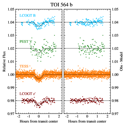
Figure 1: Left: Transits of TOI 564 b. In blue, an LCO-SSO $B$-band light curve from 2019 May 15 (§2.2.1). In green, a PEST $V$-band light curve from 2019 May 10 (§2.2.3). In orange, the detrended and phase-folded light curve of eleven transits from TESS (§2.1). In maroon, an LCO-CTIO $z^{\prime}$-band light curve from 2019 April 13 (§2.2.1). The model corresponding to each light curve’s filter is shown in grey (§4). Right: Residuals obtained by subtracting the model from the observed transits.

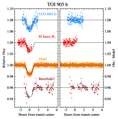
Figure 2: Left: Transits of TOI 905 b. In blue, an LCO-SSO $G$-band light curve from 2019 July 27 (§2.2.1). In red, an El Sauce $R_{\mathrm{c}}$-band light curve from 2019 July 31 (§2.2.5). In orange, the detrended and phase-folded light curve of eleven transits from TESS (§2.1). In maroon, a Brierfield $I$-band light curve from 2019 July 27 (§2.2.4). The model corresponding to each light curve’s filter is shown in grey (§4). Right: Residuals obtained by subtracting the model from the observed transits.

TOI 564 (TIC 1003831) was observed by TESS in Sector 8 by CCD 4 on Camera 2 from 2019 February 2 to 2019 February 27. TOI 905 (TIC 261867566) was observed by TESS in Sector 12 by CCD 1 on Camera 2 from 2019 May 21 to 2019 June 18. Neither target will be observed again as part of TESS’s primary mission. Basic parameters for both targets are given in Table 1.

The photometric data were analyzed with the Science Processing Operations Center (SPOC) pipeline (Jenkins et al., 2016) by NASA Ames Research Center. The data have a cadence of two-minutes, and there is a gap of six days in the case of TOI 564 and a gap of one day in the case of TOI 905. TESS’s CCD pixels have an on-sky size of 21″. The SPOC pipeline produces two types of light curves: the Simple Aperture Photometry (SAP) light curves, which are corrected for background effects; and the Pre-search Data Conditioning (PDCSAP) light curves (Smith et al., 2012; Stumpe et al., 2014), which are additionally corrected for systematics that appear in reference stars.

An automated data validation report (described in Twicken et al., 2018) was created for the PDCSAP light curve of both of our targets, revealing eleven transits on TOI 564 with a period of 1.65114 d and six transits with a period of 3.7395 d for TOI 905. This preliminary analysis gave a companion radius of $1.22\pm 0.16\,R_{\rm J}$ for TOI 905 , consistent with a hot Jupiter. For TOI 564 , the pipeline gave a companion radius of $0.49\pm 0.24\,R_{\rm J}$, but the impact parameter was extremely poorly constrained; we would later find that this impact parameter was near unity, consistent with a grazing transit, and so our ultimate measurement of the planetary radius was substantially larger than the initial estimate (see Section 4). Overall, both reports gave highly dispositive results in favor of the planetary hypothesis. The tests used included (for TOI 564 and TOI 905 respectively) the odd-even test ($2.1\sigma$ and $1.6\sigma$ difference), the weak secondary test ($3\sigma$ and $2\sigma$ for the max secondary peak), the statistical bootstrap test (extrapolated FAP $\sim 3\times 10^{-96}$ and $<10^{-97}$), the ghost diagnostic test (core-to-halo ratio of 3.6 and 5.9), and perhaps most importantly, the difference image centroid offsets from either the TIC position or the out-of-transit centroid (2″ in both cases, which is one tenth of a pixel). The difference images are also extremely clean and consistent with the difference image centroids, demonstrating that each the transit source is collocated with the target star image to within the resolution of the survey image.

To remove any stellar variability and other systematics that remained in the PDCSAP light curves, we further detrended the data using the following approach (see, e.g., Günther et al., 2017, 2018). First, we masked out the in-transit data. Then we trained a Gaussian Process (GP) model with a Matern 3/2 kernel and a white noise kernel on the out-of-transit data, using the celerite package (Foreman-Mackey et al., 2017). After constraining the hyper-parameters of the GP this way, we applied the GP to detrend the entire light curve. The resulting phase-folded TESS light curves near the transits of TOI 564 and TOI 905 are shown in orange in Figure 1 and Figure 2 respectively.

Table 1: Basic Observational Parameters

Parameter	TOI 564	TOI 905	Source
R.A. (hh:mm:ss)	08:41:10.8368	15:10:38.0821	Gaia DR2
Dec. (dd:mm:ss)	$-$16:02:10.7789	$-$71:21:41.8739	Gaia DR2
$\mu_{\alpha}$ (mas yr-1)	$-$2.508 $\pm$ 0.050	$-$25.839 $\pm$ 0.033	Gaia DR2
$\mu_{\delta}$ (mas yr-1)	$-$11.025 $\pm$ 0.04 2	$-$41.150 $\pm$ 0.051	Gaia DR2
Parallax (mas)	4.982 $\pm$ 0.031	6.274 $\pm$ 0.028	Gaia DR2
$TESS$ (mag)	10.670 $\pm$ 0.006	10.572 $\pm$ 0.006	TIC V8
$B$ (mag)	11.946 $\pm$ 0.138	12.358 $\pm$ 0.151	Tycho
$V$ (mag)	11.175 $\pm$ 0.103	11.192 $\pm$ 0.071	Tycho
$J$ (mag)	10.044 $\pm$ 0.030	9.890 $\pm$ 0.020	2MASS
$H$ (mag)	9.710 $\pm$ 0.030	9.510 $\pm$ 0.020	2MASS
$K$ (mag)	9.604 $\pm$ 0.020	9.448 $\pm$ 0.020	2MASS
$W1$ (mag)	9.562 $\pm$ 0.023	9.372 $\pm$ 0.022	AllWISE
$W2$ (mag)	9.598 $\pm$ 0.020	9.433 $\pm$ 0.019	AllWISE
$W3$ (mag)	9.587 $\pm$ 0.041	9.291 $\pm$ 0.030	AllWISE
$W4$ (mag)	—	9.151 $\pm$ 0.533	AllWISE
$G$ (mag)	11.142	11.081	Gaia DR2
$G_{BP}$ (mag)	11.527	11.509	Gaia DR2
$G_{RP}$ (mag)	10.622	10.528	Gaia DR2

2.2 Ground-Based Transit Photometry

Table 2: Ground-Based Transit Photometric Observations

Telescope	Camera	Filter	Pixel Scale	Est. PSF	Aperture Radius	Date	Duration	#	$\sigma$
			(″)	(″)	(pixel)	(UT)	(minutes)	of obs	(ppt)
TOI 564:
LCO-CTIO (1 m)	Sinistro	$z^{\prime}$	0.389	1.68	15	2019 April 13	195	165	0.9
MLAO (0.356 m)	STF-8300M	$B$	0.839	4.26	9	2019 May 2	82.2	48	12.0
PEST (0.3 m)	ST-8XME	$V$	1.23	4.1	7	2019 May 10	155	122	3.0
LCO-SSO (1 m)	Sinistro	$B$	0.389	2.04	14	2019 May 15	199	169	1.0
TOI 905:
LCO-SSO (0.4 m)	SBIG 6303	$g$	0.571	9.59	15	2019 July 27	228	278	2.5
Brierfield (0.36 m)	Moravian 16803	$I$	1.47	4.7	6	2019 July 27	452	137	1.7
El Sauce (0.36 m)	STT1603-3	$R_{c}$	1.47	4.46	6	2019 July 31	184	186	1.4

Ground-based photometric follow-up observations were used to confirm both that the transit signals detected by TESS were indeed on the correct stars (TIC 1003831 and TIC 261867566) and to ensure that the detections were robust in multiple bands. Four distinct transits of TOI 564 were observed between 2019 April 13 and 2019 May 15 in three unique bands from four ground-based telescopes. Two distinct transits of TOI 905 were observed on July 27 and July 31 in three unique bands from three ground-based telescopes. Figure 1 and Figure 2 show the light curves for each transit observed for TOI 564 and TOI 905 respectively.

We used TESS Transit Finder, which is a customized version of the Tapir software package (Jensen, 2013), to schedule all of the following photometric time-series follow-up observations. Table 2 gives a summary of the observations, which are described in detail in the following sections.

2.2.1 Las Cumbres Observatory Global Telescope

We acquired ground-based time-series follow-up photometry of full transits of TOI 564 on 2019 April 13 in $z^{\prime}$ band and on 2019 May 15 in $B$ band from two Las Cumbres Observatory Global Telescope (LCOGT) 1.0 m telescopes (Brown et al., 2013) located at Cerro Tololo Inter-American Observatory (CTIO) and Siding Spring Observatory (SSO) respectively. Additionally, we observed a full transit of TOI 905 on 2019 July 27 using the LCOGT 0.4 m telescope at SSO in $G$ band. All images were calibrated by the standard LCOGT BANZAI pipeline, and the photometric data were extracted using the AstroImageJ (AIJ) software package (Collins et al., 2017). The two 1.0 m telescopes used for TOI 564 are each equipped with a $4096\times 4096$ LCO SINISTRO camera that each have an image scale of $0\farcs 389$ px^-1. The 0.4 m telescope at SSO used an SBIG 6303 camera with an image scale of $0\farcs 571$ px^-1. For TOI 564 , 165 images were acquired during the 195 minute observation in $z^{\prime}$ band, and 169 images were acquired over the 199 minute observation in $B$ band. For the $G$-band transit of TOI 905 , 278 images were taken over 228 minutes.

The TOI 564 light curves show clear transit detections using apertures with radii $\sim 5\farcs 5$. The nearest known Gaia DR2 star is $23\arcsec$ from TOI 564 and 7.2 mag fainter. The FWHM of the target and nearby stars are $\sim$ $1\farcs 7$ and $\sim$ $2\farcs 0$ in $z$ and $B$ bands, respectively, so the follow-up aperture is negligibly contaminated by known nearby Gaia DR2 stars. The $z^{\prime}$- and $B$-band light curves show events having depths consistent with the TESS depth within uncertainties.

The TOI 905 light curve also shows a clear transit detection that is consistent with the TESS light curve using a photometric aperture with radius of $8\farcs 5$. Gaia DR2 finds there is a star that is 6.1 mag fainter located $2\farcs 2$ away from TIC 261867566.

2.2.2 Maury Lewin Astronomical Observatory

We observed a transit of TOI 564 b on 2019 May 2 from the Maury Lewin Astronomical Observatory (MLAO), a home observatory located in Glendora, California, USA, using a 0.356 m F10 Schmidt-Cassegrain Celestron C-14 Edge HD telescope with an SBIG STF-8300 detector and a $B$-band filter. The transit was observed at relatively high airmass, ranging from $\sim 2$ to $\sim 3$, which resulted in low precision ($\sim 12.0$ ppt) and a large trend in the time series data. We fitted and removed this airmass trend and found that the transit’s depth and shape was generally consistent with the other three ground-based transits, within the large error bars. Because of the lower precision of this transit observation compared to the other $B$-band transit observed by LCO-SSO, we ultimately do not include the MLAO data in the global fitting in Section 4.

2.2.3 Perth Exoplanet Survey Telescope

We observed a full transit of TOI 564 b on 2019 May 10 in $V$-band from the 0.3 m Perth Exoplanet Survey Telescope (PEST). PEST is a home observatory located near the city of Perth, Western Australia. The $1530\times 1020$ pixel SBIG ST-8XME camera has an image scale of 1$\farcs$23 px^-1 resulting in a $31\arcmin\times 21\arcmin$ field of view. Image reduction and aperture photometry were performed using the C-Munipack program coupled with custom scripts. The light curve has a precision of $\sim 3.0$ ppt, which is easily sufficient to verify that the transit depth is consistent with the other light curves.

2.2.4 Brierfield Observatory

We observed a transit of TOI 905 on 2019 July 27 in $I$ band using a 0.36 m telescope (PlaneWave CDK14) at the Brierfield Observatory, a home observatory in Brierfield, New South Wales, Australia. The detector was a Moravian 16803 camera, which provided a pixel scale of $1\farcs 47$ px^-1. Seeing conditions were average with some early high cloud limiting pre-ingress time. We observed a continuous transit using 137 images over 452 minutes. The images were reduced and measured as described in §2.2.1 with a photometric aperture of $8\farcs 8$.

2.2.5 El-Sauce

We observed the ingress and of a transit of TOI 905 on 2019 July 31 in $R_{c}$ band with a 0.36 m telescope (PlaneWave CDK14) at the El Sauce Observatory, located in Coquimbo Province, Chile. The detector was an SBIG STT1603-1 CCD with a pixel scale of $4\farcs 46$ px^-1. We acquired 186 images over 184 minutes, which were processed with AstroImageJ. Conditions were excellent with no moon or clouds. However, the camera lost its USB connection shortly before egress, so this part of the transit was not captured in this dataset.

2.3 High Angular-Resolution Observations

High angular-resolution observations were used to check both systems for close binary companions (including background stars or bound binary companions). We found that both stars have a faint companion nearby, all located within the apertures of the available photometric observations.

2.3.1 SOAR/HRCam

TOI 564 was observed using speckle interferometry on 2019 May 18 with HRCam (Tokovinin, 2018; Ziegler et al., 2019) in $I$ band on the SOAR 4.1 m telescope. The detector has a pixel scale of 15.75 mas px^-1, and the angular resolution was 63 mas. We rule out any companions above this limit (e.g., we can rule out a 5.1 mag companion at $>1$″ separation).

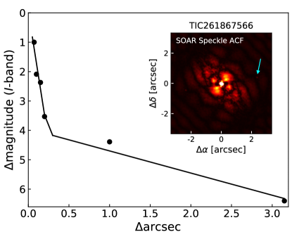
Figure 3: HRCam $I$-band contrast curve for TOI 905 with autocorrelation function (ACF) inset. Each point gives the measured $5\sigma$ contrast at various separations from the target, with a smoothing line indicating the expected shape of the contrast curve. The cyan arrow indicates the $\Delta$mag = 5.9 companion $2\farcs 28$ away from the primary star.

HRCam also conducted $I$-band speckle interferometric observations of TOI 905 on 2019 August 12 with an angular resolution of 71 mas. The ACF image in Figure 3 shows the 5$\sigma$ detection limit for this target. The HRCam reveals another source located $2\farcs 28$ away from TOI 905 that is 5.9 mag fainter in $I$ band. There is no evidence that this companion is physically associated with the system.

2.3.2 Palomar 5.1m/PHARO

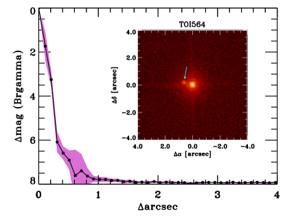
Figure 4: PHARO Br-$\gamma$ ($K$ band) contrast curve for TOI 564 with AO image inset. The cyan arrow indicates a $\Delta$mag = 3.53 companion $0\farcs 5$ away from the primary star.

TOI 564 was observed with AO using the Palomar High Angular Resolution Observer (PHARO) on the Palomar-5.1m telescope on 2019 November 10 in $H$ band (continuum) and $K$ band (narrow band Br-$\gamma$). Figure 4 reveals a stellar companion is located 0$\farcs$5 away from the primary star, with $H$ magnitude of 13.40 $\pm$ 0.04 and $K$ magnitude of 13.18 $\pm$ 0.03. These magnitudes and the $H-K$ color are consistent with a early-to-mid M dwarf binary companion with a projected separation of 100 AU, or a giant star 4–5 kpc distant. The former scenario is more parsimonious and has greater potential to create a false positive detection, so we will operate under this assumption.

2.4 Doppler Measurements

We obtained radial velocity (RV) measurements of both systems using three high-precision spectrographs. The velocities for TOI 564 (Figure 5) and TOI 905 (Figure 6) both show strong and clear Keplerian signals, which are discussed in more detail in Section 4.

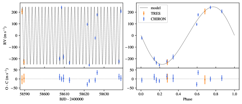
Figure 5: Left: Radial velocities of TOI 564 as a function of time, with RVs from TRES and CHIRON plotted in orange and blue respectively. In black, the modeled RV curve based on the median posterior values for parameters derived from the global fitting given in Table 5. TRES RVs were offset to minimize the rms residual from the model determined by CHIRON data. Right: Same as Left, but radial velocity is given as a function of orbital phase. The transit is centered at phase = 0; the closest RV observation to this point did not occur during the transit.

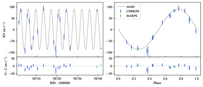
Figure 6: Left: Radial velocities of TOI 905 as a function of time, with RVs from CHIRON and HARPS plotted in blue and green respectively. In black, the modeled RV curve based on the median posterior values for parameters derived from the global fitting given in Table 5. HARPS RVs were offset to minimize the rms residual from the model determined by CHIRON data. Right: Same as Left, but radial velocity is given as a function of orbital phase. The transit occurs at phase = 0.

2.4.1 FLWO 1.5m/TRES

We obtained two spectra of TOI 564 with TRES (Fűrész et al., 2008) on the 1.5 m Tillinghast Reflector telescope at Fred L. Whipple Observatory (FLWO) on Mount Hopkins, AZ, on 2019 April 15 and 16. TRES is an $R\sim 44,000$ echelle spectrograph with a precision of $\sim$10 to 15 m $\mathrm{s^{-1}}$. Spectra are calibrated using a pair of ThAr lamp exposures flanking each set of science exposures. Observations used exposure times of $\sim$ 20 minutes, which yielded a S/N per resolution element of $\sim 32$ at 5110 Å. TRES has an on-sky fiber radius of 1$\farcs$15.

The reduction and analysis procedures are described in Buchhave et al. (2010). To summarize, the 2D spectra are optimally extracted and then cross correlated order-by-order using the stronger of the two observations as the template. The radial velocities are determined from a fit to the summed cross-correlation function (CCF), and the internal errors at each epoch are estimated from the standard deviation of the radial velocities derived from the CCF of each order. We also track the instrumental zero point and instrumental precision by monitoring RV standards every night and use this analysis to adjust the RVs and uncertainties. While the internal errors dominate for this star, we do inflate the internal errors by adding the instrumental uncertainty ($\sim$ 10 m $\mathrm{s^{-1}}$) in quadrature. The RVs and uncertainties reported in Table 3 include these corrections.

2.4.2 SMARTS 1.5m/CHIRON

Table 3: Radial Velocity Measurements

BJD - 2400000	RV	$\sigma_{\mathrm{{RV}}}$	BIS	$\sigma_{\mathrm{{BIS}}}$	FWHM	$\sigma_{\mathrm{{FWHM}}}$	S/N	Target	Instrument
	($\mathrm{m\ s^{-1}}$)	($\mathrm{m\ s^{-1}}$)	($\mathrm{m\ s^{-1}}$)	($\mathrm{m\ s^{-1}}$)	($\mathrm{km\ s^{-1}}$)	($\mathrm{km\ s^{-1}}$)
58588.6801	413.0	24.4	6.9	10.2	—	—	31.0	TOI 564	TRES
58589.6683	-22.8	24.4	-6.9	10.2	—	—	34.2	TOI 564	TRES
58607.5990	-198.7	16.7	13.7	10.5	10.124	0.153	37.1	TOI 564	CHIRON
58608.5907	240.8	13.6	8.6	9.1	10.441	0.118	47.6	TOI 564	CHIRON
58609.5843	-184.6	20.8	27.4	12.9	9.501	0.163	30.9	TOI 564	CHIRON
58612.5903	-234.5	15.3	-12.0	15.2	10.162	0.129	38.7	TOI 564	CHIRON
58621.5585	95.6	12.3	12.0	10.2	10.088	0.116	39.8	TOI 564	CHIRON
58622.5497	-254.5	10.9	13.7	9.6	10.107	0.122	39.4	TOI 564	CHIRON
58625.5427	-22.0	13.2	30.9	10.9	10.243	0.128	38.4	TOI 564	CHIRON
58626.5368	177.7	13.1	24.0	8.1	10.405	0.125	48.5	TOI 564	CHIRON
58637.5439	-223.5	15.9	18.9	13.5	10.241	0.134	43.0	TOI 564	CHIRON
58638.5128	207.4	15.6	22.3	15.9	10.195	0.112	39.9	TOI 564	CHIRON
58701.4994	32.2	9.7	1.3	16.5	9.953	0.073	46.8	TOI 905	CHIRON
58702.5685	83.1	9.7	-2.6	14.1	9.885	0.079	42.2	TOI 905	CHIRON
58704.4989	-93.5	11.3	-16.7	19.2	9.747	0.100	36.3	TOI 905	CHIRON
58705.5794	61.7	10.3	-14.1	18.9	9.864	0.094	41.1	TOI 905	CHIRON
58706.5228	39.5	12.3	-7.7	22.4	9.842	0.087	38.1	TOI 905	CHIRON
58707.5088	-78.8	10.2	-18.0	13.6	9.804	0.085	39.8	TOI 905	CHIRON
58708.5073	-36.4	8.8	-27.0	16.4	9.860	0.087	44.7	TOI 905	CHIRON
58710.5776	-5.7	12.4	0.0	20.4	9.766	0.096	38.8	TOI 905	CHIRON
58713.5038	94.3	11.6	10.3	11.1	9.917	0.088	44.4	TOI 905	CHIRON
58718.5033	-54.9	9.4	-12.9	16.5	9.984	0.083	45.8	TOI 905	CHIRON
58719.5102	-94.1	21.8	-78.4	31.2	9.598	0.108	28.9	TOI 905	CHIRON
58720.5899	61.4	9.4	6.4	16.8	9.951	0.091	44.6	TOI 905	CHIRON
58721.4963	46.2	10.7	1.3	14.9	9.937	0.081	44.1	TOI 905	CHIRON
58723.4948	-32.1	10.9	-12.9	25.0	9.826	0.090	38.9	TOI 905	CHIRON
58724.4959	82.3	7.3	9.0	14.4	9.968	0.087	45.4	TOI 905	CHIRON
58726.4917	-81.9	11.8	38.6	20.1	9.871	0.085	40.2	TOI 905	CHIRON
58739.513	83.1	4.845	43.4	—	6.664	—	39.9	TOI 905	HARPS
58741.512	-82.5	4.054	15.9	—	6.673	—	44.5	TOI 905	HARPS

We collected ten spectra of TOI 564 with CHIRON (Tokovinin et al., 2013), a fiber-fed spectrograph on the SMARTS 1.5 m telescope at Cerro Tololo, Chile, between 2019 May 4 and 2019 June 4, and sixteen spectra of TOI 905 between 5 August 2019 and 30 August 2019. The short period of both planet candidates allowed us to quickly verify that the star showed an RV signal consistent with a planetary-mass companion by observing each star near the quadrature points implied by the transit ephemerides and the assumption of a circular orbit. We then proceeded to fill out the phase curve of each planet’s orbit.

We used CHIRON’s $R=80,000$ slicer mode for all observations, which provides substantially higher instrumental throughput when compared to the slit or narrow slit mode (relative efficiencies of the modes are 0.82, 0.25, and 0.11, respectively; Tokovinin et al., 2013). In addition, we did not use the iodine cell, which would have absorbed about half of the stellar light in the $\sim$ 5000-6100 Å  region. Each observation used an exposure time of 25 minutes, which provided a typical S/N per resolution element of $\sim 40$ at 5500 Å. The on-sky fiber radius of CHIRON is 1$\farcs$35.

The RVs were derived closely following the procedure described in Jones et al. (2017) and Wang et al. (2019). Briefly, we first built a template by stacking the individual CHIRON spectra, after shifting all of them to a common rest frame. We then computed the cross-correlation-function (CCF) between each observed spectrum and the template. The CCF was then fitted with a Gaussian function plus a linear trend. The velocity corresponding to the maximum of the Gaussian fit corresponds to the observed radial velocity. We applied this method to a total of 33 orders, covering the wavelength range of $\sim$ 4700 - 6500 Å. Since CHIRON is not equipped with a simultaneous calibration fiber, we obtained a ThAr lamp immediately before each science observations. The CHIRON pipeline therefore recomputes a new wavelength solution from this calibration observation, thus correcting for the instrumental drift. Using this method, we achieve a long-term stability better than 10 m s^-1, which has been tested using RV standard stars. The final RV at each epoch is obtained from the median in the individual order velocities, after applying a 3$\sigma$ rejection method. The corresponding uncertainty is computed from the error in the mean of the non-rejected velocities (see more details in Jones et al. 2017). The typical RV error found was about 15 $\mathrm{m\ s^{-1}}$. Finally, we also computed the bisector inverse slope (BIS) and full-width-at-half-maximum (FWHM) of the CCF. The full results of the CCF analysis are given in Table 3, including the BIS and FWHM diagnostics.

2.4.3 ESO 3.6m/HARPS

We collected two spectra of TOI 905 with the High Accuracy Radial velocity Planet Searcher (HARPS) (Mayor et al., 2003) at the ESO 3.6 meter telescope. HARPS has a spectral resolution of $R=115,000$ and a fiber with an on-sky radius of 0$\farcs$5. Exposure times were 25 minutes, achieving S/N $\sim$ 42 at 5500 Å.

Our motivation in collecting HARPS spectra was to test if the semiamplitude of the signal was consistent between HARPS and CHIRON, which have sky fibers of 0$\farcs$5 and 1$\farcs$35 respectively. If there is potential RV contamination from the nearby star 2$\farcs$28 away (§2.3.1), then the Doppler semiamplitude should be different between the instruments. Figure 6 shows that when the HARPS RVs are offset to match CHIRON, they agree closely.

3 Host Star Characterization

It is well-understood that when the transit and RV techniques are used for planet characterization, we can only know the planet as well as we know the star. We derived physical and atmospheric parameters for TOI 564 and TOI 905 using several independent methodologies and data sets that are described in the following subsections (the stellar parameters determined by EXOFASTv2 are described later in Section 4).

We find that among the values probed by multiple methods there is generally agreement within 1–2$\sigma$, giving us greater confidence in their collective veracity. Both stars are G-type main sequence stars, which are roughly Sun-like in their mass, radius, and temperature. Both stars are metal-rich. A summary of the parameters derived is shown in Table 4.

Table 4: Stellar Parameters

Parameter	FLWO 1.5m/TRES	SMARTS 1.5m/CHIRON	SED (Stassun)	SED (EXOFASTv2)
TOI 564:
$M_{*}$ ($\,M_{\sun}$)	—	$1.1\pm 0.1$	$1.06\pm 0.06$	$0.998^{+0.068}_{-0.057}$
$R_{*}$ ($\,R_{\sun}$)	—	$1.04\pm 0.05$	$1.092\pm 0.020$	$1.088\pm 0.014$
$L_{*}$ ($\,L_{\sun}$)	—	$1.06\pm 0.11$	—	$1.078^{+0.028}_{-0.030}$
$T_{\rm eff}$ (K)	$5666\pm 50$	$5780\pm 100$	—	$5640^{+34}_{-37}$
$\log{g_{*}}$ (cgs)	$4.41\pm 0.10$	$4.23\pm 0.20$	—	$4.364^{+0.032}_{-0.028}$
$V\ \mathrm{sin}\ i$ ($\mathrm{km\ s^{-1}}$)	$3.54\pm 0.5$	—	—	—
$\left[{\rm Fe}/{\rm H}\right]$ (dex)	$0.15\pm 0.08$	$0.34\pm 0.20$	—	$0.143^{+0.076}_{-0.078}$
Age (Gyr)	—	—	—	$7.3^{+3.5}_{-3.6}$
TOI 905:
$M_{*}$ ($\,M_{\sun}$)	—	$0.85\pm 0.10$	$1.15\pm 0.07$	$0.968^{+0.061}_{-0.068}$
$R_{*}$ ($\,R_{\sun}$)	—	$1.14\pm 0.03$	$0.964\pm 0.052$	$0.918^{+0.038}_{-0.036}$
$L_{*}$ ($\,L_{\sun}$)	—	$0.93\pm 0.05$	—	$0.730^{+0.12}_{-0.095}$
$T_{\rm eff}$ (K)	—	$5300\pm 100$	—	$5570^{+150}_{-140}$
$\log{g_{*}}$ (cgs)	—	$3.94\pm 0.20$	—	$4.498^{+0.025}_{-0.027}$
$V\ \mathrm{sin}\ i$ ($\mathrm{km\ s^{-1}}$)	—	—	—	—
$\left[{\rm Fe}/{\rm H}\right]$ (dex)	—	$0.20\pm 0.10$	—	$0.14^{+0.22}_{-0.18}$
Age (Gyr)	—	—	—	$3.4^{+3.8}_{-2.3}$

3.1 Results from FLWO 1.5m/TRES

We derived spectral parameters from the TRES spectra of TOI 564 using the Spectral Parameter Classification (SPC) tool (Buchhave et al., 2012). SPC cross correlates the observed spectrum against a grid of synthetic spectra based on Kurucz atmospheric models (Kurucz, 1993). $T_{\rm eff}$, $\log{g_{*}}$, $\left[{\rm Fe}/{\rm H}\right]$, and $V\ \mathrm{sin}\ i$ are allowed to vary as free parameters. We find that $T_{\rm eff}=5666\pm 50$ K, $\log{g_{*}}=4.41\pm 0.10$, $\left[{\rm Fe}/{\rm H}\right]=0.15\pm 0.08$, and $V\ \mathrm{sin}\ i=3.54\pm 0.5$ km $\mathrm{s^{-1}}$.

3.2 Results from SMARTS 1.5m/CHIRON

We derive the atmospheric parameters of both TOI 564 and TOI 905 following the method presented in Jones et al. (2011) and Wang et al. (2019). We used the CHIRON template (see §2.4) to measure the equivalent width (EW) of a total of 110 Fe i and 20 Fe ii lines in the weak-line regime (EW $<$ 150 Å). The EWs were measured after fitting the local continuum using the ARES2 v2 automatic tool (Sousa et al., 2015).

We then solved the radiative transfer equation by imposing local excitation and ionization equilibrium (Boltzmann and Saha equations, respectively) and assuming a solar metal content distribution. For this, we used the MOOG code (Sneden, 1973) along with the Kurucz (1993) stellar atmosphere models. For models with different $T_{\rm eff}$ , $\log{g_{*}}$ , and $\left[{\rm Fe}/{\rm H}\right]$ , we iterate until no dependence between the excitation potential and wavelength of the individual lines with the model abundance is found, and with the constraint that the model abundance is the same for both the Fe i and Fe ii lines. We note that the microturbulence velocity ($v_{t}$) is a free parameter in the fit. Using this method, we obtained the following atmospheric parameters for TOI 564: $T_{\rm eff}$ = 5780 $\pm$ 100 K, $\log{g_{*}}=4.23\pm 0.20$ dex, $\left[{\rm Fe}/{\rm H}\right]=0.34\pm 0.20$ and $v_{t}$ = 0.75 $\pm$ 0.10 km s^-1. For TOI 905 , we found: $T_{\rm eff}$ = 5300 $\pm$ 100 K, $\log{g_{*}}=3.94\pm 0.20$ dex, and $\left[{\rm Fe}/{\rm H}\right]=0.20\pm 0.10$.

We adopted a value of A_v = 0.10 $\pm$ 0.10 for the interstellar reddening to derive corrected visual apparent magnitudes. We also correct the Gaia parallax by a systematic offset of 82 $\pm$ 32 $\mu\arcsec$ (Stassun & Torres, 2018) to obtain $\varpi$ = 5.0638 $\pm$ 0.04738 and $6.66^{+0.32}_{-0.30}$ for TOI 564 and TOI 905 respectively. Using the bolometric corrections presented in Alonso et al. (1999), we calculate a stellar luminosity of L_⋆ = 1.06 $\pm$ 0.11 $\,L_{\sun}$. Finally, by comparing the L_⋆, $T_{\rm eff}$ , and [Fe/H] with the PARSEC evolutionary tracks (Bressan et al., 2012), we derived a stellar mass and radius of 1.1 $\pm$ 0.1 $\,M_{\sun}$ and 1.04 $\pm$ 0.05 $\,R_{\sun}$ respectively for TOI 564 , and 0.85 $\pm$ 0.10 $\,M_{\sun}$ and 1.14 $\pm$ 0.03 $\,R_{\sun}$ for TOI 905.

3.3 Results from independent SED fitting

Although we will compute stellar parameters based on the broadband spectral energy distribution (SED) in a global analysis using EXOFASTv2 (see §4), we also perform a separate SED analysis as an independent check on the derived stellar parameters. Here, we use the SED together with the Gaia DR2 parallax in order to determine an empirical measurement of the stellar radius following the procedures described in Stassun & Torres (2016); Stassun et al. (2017, 2018). We pulled the $B_{T}V_{T}$ magnitudes from Tycho-2, the $BVgri$ magnitudes from APASS, the $JHK_{S}$ magnitudes from 2MASS, the W1–W4 magnitudes from WISE, the $G$ magnitude from Gaia, and the NUV magnitude from GALEX. Together, the available photometry spans the full stellar SED over the wavelength range 0.2–22 $\mu$m for TOI 564 and 0.4–22 $\mu$m for TOI 905 (see Figure 7).

We performed a fit using Kurucz stellar atmosphere models. The priors on effective temperature ($T_{\rm eff}$), surface gravity ($\log{g_{*}}$), and metallicity ($\left[{\rm Fe}/{\rm H}\right]$) were from spectroscopically determined values for TOI 564 and from the values provided in the TIC (Stassun et al., 2018) for TOI 905. The remaining free parameter is the extinction ($A_{V}$), which we restricted to the maximum line-of-sight value from the dust maps of Schlegel et al. (1998). The resulting fits are excellent (Figure 7) with a reduced $\chi^{2}$ of 3.8 when excluding the NUV flux, which suggests mild chromospheric activity. The best-fit extinction is $A_{V}=0.03_{-0.03}^{+0.11}$. Integrating the (unreddened) model SED gives the bolometric flux at Earth of $F_{\rm bol}=9.04\pm 0.32\times 10^{-10}$ erg s cm^-2. Taking the $F_{\rm bol}$ and $T_{\rm eff}$ together with the Gaia DR2 parallax, adjusted by $+0.08$ mas to account for the systematic offset reported by Stassun & Torres (2018), gives the stellar radius as $R=1.092\pm 0.020$ R_⊙. Finally, estimating the stellar mass from the empirical relations of Torres et al. (2010) gives $M=1.06\pm 0.06\ M_{\odot}$, which with the radius gives the mean stellar density $\rho=1.15\pm 0.12$ g cm^-3.

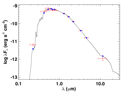
Figure 7: Spectral energy distribution (SED). Red symbols represent the observed photometric measurements, where the horizontal bars represent the effective width of the passband. Blue symbols are the model fluxes from the best-fit Kurucz atmosphere model (black).

4 Planetary System Parameters from Global Analysis

We model planetary system and stellar parameters, as in Wang et al. (2019), using EXOFASTv2 (Eastman et al., 2013; Eastman, 2017; Eastman et al., 2019), a fast and powerful exoplanetary fitting suite. We performed a global simultaneous analyses of both systems using light curves from TESS, LCO-CTIO, PEST, LCO-SSO, Brierfield, El-Sauce, RVs from CHIRON, and stellar spectral energy distributions. We did not include the MLAO $B$-band light curve for TOI 564 because of its lower precision compared to the LCO-SSO $B$-band light curve. We also did not include the two TRES or the two HARPS RVs, which, on their own, were not informative enough to justify introducing an additional two degrees of freedom to the fitting (namely instrumental offset and instrumental jitter); nevertheless, we note that each of these pairs of RVs were consistent with the CHIRON RVs in both systems.

During the global fitting, we applied the quadratic limb darkening law and performed a coefficients fit with a TESS-band prior based on the relation of stellar parameters ($\log{g_{*}}$, $T_{\rm eff}$, and $\left[{\rm Fe}/{\rm H}\right]$) and coefficients (Claret et al., 2018). The corrected Gaia parallax for each target (§3.2) is adopted as the Gaussian prior imposed on the Gaia DR2 parallaxes. An upper limit is imposed on the $V$-band extinction of 0.14 from Schlafly & Finkbeiner (2011).

To constrain each SED, we utilized the photometry from Tycho (Høg et al., 2000), 2MASS $\it JHK$ (Cutri et al., 2003), AllWISE (Cutri et al., 2013), and Gaia DR2 (Gaia Collaboration et al., 2018); these magnitudes are given in Table 1. With the initial value of $T_{\rm eff}$ ($5780\pm 100$ K and $5300\pm 100$ K for TOI 564 and TOI 905 respectively) derived from §3.2, we utilized the available spectral energy distribution and the MIST stellar-evolutionary models (Dotter, 2016; Choi et al., 2016) to further constrain the stellar parameters.

We began the fit with relatively standard Hot Jupiter starting conditions, but, as suggested by Eastman et al. (2019), we iterated with relatively short MCMC runs with parallel tempering enabled to refine the starting conditions and ensure that the AMOEBA optimizer could find a good solution to all constraints simultaneously. This is not strictly required, but can dramatically improve the efficiency of EXOFASTv2. Once we found a good solution, we ran a final fit until the standard criteria (both the number of independent draws being greater than 1000 and a Gelman-Rubin statistic of less than 1.01 for all parameters) were satisfied six consecutive times, indicating that the chains were considered to be well-mixed (Eastman et al., 2013).

Table 5 summarizes the relevant parameters reported by EXOFASTv2, with median value and 68% confidence intervals (CI) for each posterior. TOI 564 is found to be Sun-like, with a mass of $0.998^{+0.068}_{-0.057}$ $\,M_{\sun}$, radius of $1.088\pm 0.014$ $\,R_{\sun}$, and $T_{\rm eff}$ of $5640^{+34}_{-37}$ K. TOI 905 is slightly smaller with a mass of $0.968^{+0.061}_{-0.068}$ $\,M_{\sun}$, radius of $0.918^{+0.038}_{-0.036}$ $\,R_{\sun}$, and $T_{\rm eff}$ of $5570^{+150}_{-140}$. The two stars are each metal-rich with $\left[{\rm Fe}/{\rm H}\right]=0.143^{+0.076}_{-0.078}$ and $0.14^{+0.22}_{-0.18}$ dex, respectively, which is consistent with our understanding of hot Jupiter host stars (Fischer & Valenti, 2005).

The masses of both planets are determined from the CHIRON RVs and the modeled inclinations. TOI 564 b has a mass of $1.463^{+0.10}_{-0.096}\,M_{\rm J}$, and TOI 905 b has a mass of $0.667^{+0.042}_{-0.041}\,M_{\rm J}$. The RV curves corresponding to the median posterior values for the relevant orbital and planetary parameters are shown in Figure 5 and Figure 6 in black.

The transit models based on the median posterior values for each planet and photometric band are plotted in Figure 1 and Figure 2. EXOFASTv2 finds a median radius and 68% CI of TOI 905 b of $1.171^{+0.053}_{-0.051}\,R_{\rm J}$. The radius of TOI 564 b is far more difficult to constrain; we find a median and 68% CI of $1.02^{+0.71}_{-0.29}$ $\,R_{\rm J}$. This value is very sensitive to small changes in the the impact parameter, which we determine to be $0.994^{+0.083}_{-0.049}$ with an inclination of $78.38^{+0.71}_{-0.85}$ degrees. This high impact parameter corresponds to a grazing transit scenario, and it creates a tricky interplay between the modeled $R_{p}$ and $b$.

The uncertainties in the radius of TOI 564 b are compounded in the median and 68% CI of the bulk density estimate of $1.7^{+3.1}_{-1.4}$ g cm^-3. The density of TOI 905 b is more precisely determined to be $0.515^{+0.063}_{-0.057}$ g cm^-3. We find that the eccentricity is consistent with 0 with a median value and 68% CI of $0.072^{+0.083}_{-0.050}$. Indeed, a circular orbit is to be expected for this planet based on the rapid tidal circulation timescale (as computed by Adams & Laughlin, 2006, with $Q_{*}=10^{6}$) of $0.043^{+0.20}_{-0.040}$ Gyr, which is very short compared to the stellar age of $7.3^{+3.6}_{-3.5}$ Gyr. TOI 905 b also has an eccentricity that is consistent with a circular orbit: $0.024^{+0.025}_{−0.017}$. The tidal circularization timescale for this planet is $0.323^{+0.063}_{−0.054}$ Gyr.

5 Discussion

5.1 Consideration of False Positive Scenarios

False positive scenarios such as background eclipsing binaries, or nearby eclipsing binaries can masquerade as giant planets in transit data and occasionally also in radial velocity data as well (e.g., Torres et al., 2004). We should be especially wary of these scenarios given that nearby stars were detected for both of these primary host stars. Here we explicitly discuss several tests for false positive scenarios. Taken together, we find that the lines of evidence collectively demonstrate the planetary nature of these bodies.

5.1.1 RV CCF Correlations

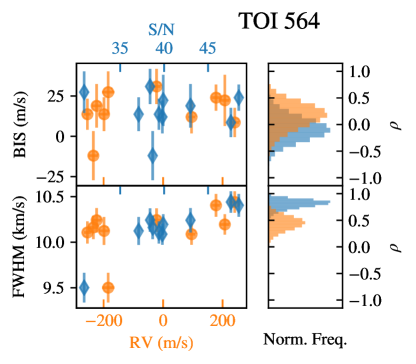
Figure 8: CCF correlations for the CHIRON observations of TOI 564. Left: BIS (top) and the FWHM (bottom) of the CCF are each plotted vs. both RV (orange circles) and vs. S/N (blue diamonds). Right: histograms of the Pearson correlation coefficient ($\rho$) values between either BIS (top) or FWHM (bottom) vs. RV (orange) or S/N (blue), based on a resampling of the data on the left.

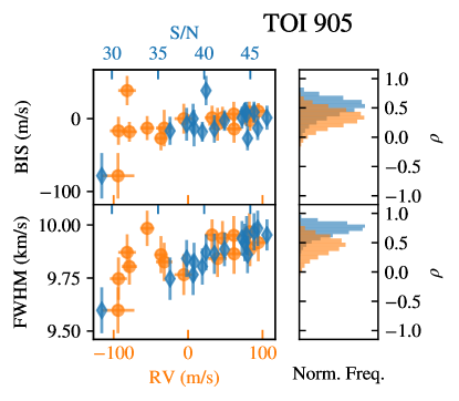
Figure 9: Same as Figure 8, but for TOI 905.

Strong correlations between the CCF BIS or CCF FWHM and RV can raise concerns of stellar activity masquerading as planet signals. Additionally, a marginally resolved double-lined binary can cause RV-correlated CCF variations while producing a false positive diluted planetary transit signal.

We examined the BIS and FWHM for possible linear correlations with both the RVs using the Pearson correlation coefficient, $\rho$. We calculated $\rho$ over 100,000 realizations of the data resampled from a bivarate normal distribution using the $1\sigma$ errors in both quantities. The results are seen in orange in Figure 8 and Figure 9 for TOI 564 and TOI 905 respectively. TOI 564 shows no correlations between BIS and RV, but the zero correlation case for FWHM and RV is excluded with high confidence. For TOI 905, there is a marginally significant correlation between BIS and RV, and, again, a highly significant non-zero correlation for FWHM and RV.

These correlations are potentially concerning. However, we believe that the correlations are better explained as manifestations of systematic errors in our reduction pipeline that increase with low S/N. The correlations between the CCF and S/N are also in Figure 8 and Figure 9 plotted in blue. We find that in each of the cases where zero correlation was ruled out between the RVs and BIS or FWHM, the correlation was many-$\sigma$ stronger when compared to S/N instead. For instance, for TOI 905 the FWHM and RV have non-zero correlation at the $3.3\sigma$-level, whereas the FWHM and S/N have a non-zero correlation at the $9.5\sigma$-level. Therefore, we do not conclude that we have observed statistically significant astrophysically produced CCF-RV correlations, and we so fail to refute the planetary interpretation.

5.1.2 TODCOR Analysis

Since a potentially significant bisector correlation was detected in the CCFs of TOI 905, we further analyzed these spectra using TODCOR (Zucker, & Mazeh, 1994). We searched for additional RV components separated by less than $\sim$15 km/s in a procedure similar to the one applied in the analysis of the wide binary companion of HD 202772 (Wang et al., 2019). The search revealed no significant secondary velocity signal. TODCOR confirmed the RV signal was on target, and that it was not induced by a blend with another component. The upper limit on the relative flux contribution of another star in the system was estimated to be $\sim$5–10%.

An independent reduction of the RVs obtained with TODCOR and BIS measurements obtained with UNICOR (Engel et al., 2017) reproduced the observed RV semi-amplitude using the reduction described in §2.4.2, but not the strong CCF correlations found by the CHIRON reduction; this reinforces our conclusion that the correlations discussed in §5.1.1 are dominated by reduction issues and are not astrophysical in origin.

5.1.3 Bounds for Inclination of M-dwarf Binary

The apparent grazing transit of TOI 564 combined with the existence of a likely M-dwarf companion in the system raises the possibility that the system may consistent of a close M-dwarf binary pair that orbit the G star in a hierarchical triple system. In this scenario, an eclipse of the M-dwarf pair would be contaminated by the bright G star, leading to a spurious planetary transit signal, and the RVs of the system would similarly consist of high amplitude RVs from the M-dwarf pair that are diluted by the G star.

The agreement of the 1.65 day period between the transit and RV observations rule out a mutual-eclipse scenario in a hypothetical M-dwarf pair; such a binary must only experience one eclipse per orbit. A single-eclipse orbit necessitates an orbit that has non-zero eccentricity. The RVs for this system constrain the eccentricity to $0.072^{+0.083}_{-0.050}$.

We simulated this geometry, assuming the two M-dwarfs each were 0.3 $\,M_{\sun}$ and 0.3 $\,R_{\sun}$. The semi-major axis is therefore 0.0231 AU. We find that an inclination of $82.5^{\circ}<i<83.5^{\circ}$ is required to produce exactly one eclipse in this scenario. Although possible, it would be unlikely a priori to find a two-body system that falls within such a tight inclination bounds.

5.1.4 Color Dependence

In the hierarchical triple system scenario for TOI 564 explored in §5.1.3, an eclipse of an M dwarf would produce transits that are deeper in redder wavelengths, in accordance with the cool stars’ colors. A typical M3 star has $B-V=1.5$, compared to the primary star’s measured $B-V$ value of 0.77. This color difference between the two spectral types corresponds to a factor of $\sim$2 difference in the expected transit depths between $B$ and $V$ if the M dwarf is being eclipsed. Instead, we find that there is only a $\sim$ 0.1 ppt depth difference between the transit depth in $B$ and $V$ for this star; indeed, all transit depths only vary by 0.5 ppt between $B$ and $z^{\prime}$.

The hierarchical triple system scenario would similarly cause a color dependence in the RVs, due to a varying amount of spectral contamination from the red to the blue wavelengths. We found that RVs as a function of spectral order were distributed randomly, and there is no sign of any color dependence.

5.2 Planets in Context

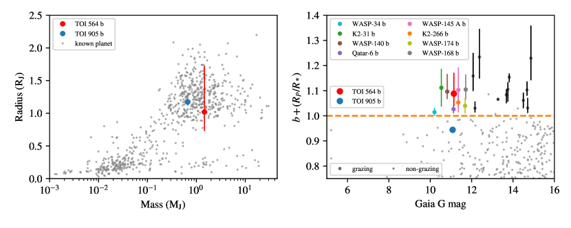
Figure 10: Newly discovered planets TOI 564 b and TOI 905 b compared to known planets that have parameters published on the NASA Exoplanet Archive (Akeson et al., 2013). Left: Mass-radius relation for confirmed transiting planets, with TOI 564 b and TOI 905 b in blue and red, respectively, with 68% confidence indicated (errors omitted for known planets). The both masses and radii are typical of gas giant planets. Right: The grazing transit condition vs. $G$ (Gaia) magnitude. The orange dashed line indicates the threshold above which transits become grazing. Planets with grazing transit probability greater than 84% (i.e., based on published $1\sigma$ uncertainties) are labeled in various colors or in black. TOI 564 is among the brightest stars known to host a grazing transiting planet with high confidence.

TOI 564 b and TOI 905 b are each classical transiting hot Jupiters, orbiting G-type host stars with (respectively) periods of 1.65 d and 3.74 d, masses of 1.46 and 0.67 $\,M_{\rm J}$, and radii of 1.02 and 1.17 $\,R_{\rm J}$. Figure 10 (left) shows that these planets’ masses and radii compared to other transiting planets. TOI 905 b sits comfortably among previously discovered gas giants, as does TOI 564 b, even near the extremes of its 68% CI radius values. Given the nature of the grazing transit, however, TOI 564 b could be much larger (commensurate with a greater value of the impact parameter).

Based on TOI 564 b’s calculated $T_{\mathrm{eq}}$ of $1714^{+20}_{-21}$ K, the fact this is a gas-giant mass planet, and comparison to other known hot Jupiters (see, e.g., Wu et al., 2018), it is likely that TOI 564 b is inflated. A typical hot Jupiter at this $T_{eq}$ would have a radius of $\sim$1.3 $\,R_{\rm J}$, which is consistent within our measured radius of $1.02^{+0.71}_{-0.29}$ $\,R_{\rm J}$. If TOI 564 b’s radius fell at the low end of the 68% CI derived from EXOFASTv2, it would be one of the least inflated giant planets given its temperature. Given the difficulties in modeling a grazing transit, we suggest that TOI 564 bś radius should be viewed cautiously as a lower-bound. TOI 905 b has a calculated $T_{\mathrm{eq}}$ of $1192^{+39}_{-36}$ K, which puts it just past the critical temperature of inflation ($1123.7\pm 3.3$ K) found by Wu et al. (2018). At 1.17 $\,R_{\rm J}$, this planet is fully consistent with known giant planets at this $T_{\mathrm{eq}}$.

The high impact parameter, $b=0.994^{+0.083}_{-0.049}$, makes TOI 564 b stand out in Figure 10 (right), which plots the grazing transit condition vs. $Gaia$ magnitude. TOI 564 is among the brightest stars known to host a grazing transiting planet. This makes it one of the most attractive targets for long term monitoring in searches for transit depth variations and impact parameters variations that could reveal the presence of non-transiting planets or exomoons (Kipping, 2009, 2010). The grazing transits also offer an opportunity to search for exotrojan asteroids (e.g., Lillo-Box et al., 2018) by exploiting the sensitivity of the orbit of TOI 564 b to co-orbital perturbations.

Miralda-Escudé (2002) examines this possibility using the 51 Peg system (Mayor, & Queloz, 1995) as an example. A close-in hot Jupiter will experience both a precession in its periastron as well as a precession in its line of nodes when an additional planet is present in the system. Miralda-Escudé (2002) finds, for example, that in the case of an Earth-mass planet located at $a=0.2$ AU with an inclination of $45^{\circ}$, 51 Peg b would experience transit duration changes of 1 s $\mathrm{yr^{-1}}$, which would be detectable over many years of observation. However, the grazing nature of TOI 564 b’s transit means that any line-of-nodes precession will manifest itself as a change to the already-high impact parameter, upon which the transit duration and transit depth are both extremely sensitive. These changes can be used to dynamically constrain the presence of smaller and more distant planetary companions, which are of particular interest because they can help address hot Jupiter formation and evolution scenarios.

We find that TOI 564 b is unlikely to be eclipsed by its host star, with the 68% CI eclipse duration being $0.000^{+0.021}_{-0.00}$ d. However, TOI 905 b is expected to be eclipsed by its host, with an eclipse duration of $0.0845^{+0.0011}_{-0.0015}$ d. There is therefore potential for further study of this planet’s thermal emission and atmospheric characterization.

We simulated the Rossiter-McLaughlin effect using ExOSAM (see, Addison et al., 2018) for both TOI 564 b and TOI 905 b. Following the results of the TRES observations, we set set $V\ \mathrm{sin}\ i=\mathrm{3.5\ km\ s^{-1}}$ for TOI 564, and we consider two cases: an aligned orbit with $\lambda=0^{\circ}$, and with a polar orbit with $\lambda=90^{\circ}$. For an aligned orbit, the predicted semi-amplitude of the velocity anomaly is $\mathrm{\sim 8\ m\ s^{-1}}$. In the case where $\lambda\sim 90^{\circ}$ and the star has a non-trivial vsini, either the red-shifted or the blue-shifted limb of the star will be occulted, which will result in a measurable, fully asymmetric Rossiter-McLaughlin signal of $\mathrm{\sim 7\ m\ s^{-1}}$. With a transit duration of just over one hour, it would be readily possible for a large-aperture telescope with a spectrograph attaining better than $\mathrm{4\ m\ s^{-1}}$ precision with a cadence of $\sim 10$ min, (e.g., Keck/HIRES, Vogt et al. 1994; Magellan/PFS, Crane et al. 2006), to measure $\lambda$ in this system. We do not have measurements of $V\ \mathrm{sin}\ i$ for TOI 905, but the deeper transit would probably create a larger RM signal; e.g., arbitrarily assuming the same $V\ \mathrm{sin}\ i$ of $\mathrm{3.5\ km\ s^{-1}}$, we find that TOI 905 b would have an RM semi-amplitude of $\mathrm{\sim 23\ m\ s^{-1}}$ for an aligned orbit.

The confirmation of this grazing transiting planet may also serve as a valuable data point in informing the mystery behind the paucity in detections of exoplanets with grazing transits, even after accounting for the detection biases resulting from their shallower and shorter transits. Polar star spots have been observed on both main sequence stars (Jeffers et al., 2002) and active, rapid rotators (Schuessler & Solanki, 1992). These spots reduce the background flux of the region occulted by planets exhibiting a grazing transit, which necessarily transit at high latitude in the default case of $\lambda=0^{\circ}$. Oshagh et al. (2015) posits that this effect could be responsible for the dearth of grazing transiting planet detections by Kepler. If TOI 564 b is indeed in an aligned orbit, then its transits must cross the stellar pole (because of the grazing transits), which would grant us the opportunity to study this phenomenon.

6 Summary and Conclusion

We report the discovery and confirmation of two new hot Jupiters identified by TESS: TOI 564 b and TOI 905 b. TOI 564 b is noteworthy in that it displays a grazing transit across its Sun-like host star in over its 1.65 d orbit. Both targets are main sequence G stars that are relatively bright ($V\sim 11$), making them good targets for follow-up characterization.

Both planets were validated based on the TESS light curves, ground-based photometry in three different filters, and robust radial velocity detections by CHIRON. Both stars were observed with speckle interferometry (HRCam/SOAR) and TOI 564 was also observed with PHARO/Palomar AO. TOI 564 is a probable binary system, with an M-dwarf companion at a projected distance of $\sim$100 AU.

We conducted multiple independent measurements of the host stars’ stellar parameters using the high resolution CHIRON and TRES spectra as well as an SED analysis and found a general agreement between the derived parameters. Using the EXOFASTv2 planet fitting suite, we ran a global analysis by simultaneously fitting the transit and RV data with a Markov chain Monte Carlo. TOI 564 b’s impact parameter was found to be near unity, diminishing our ability to constrain its radius, but its mass, as well as the radius and mass of TOI 905 b, was measured with high precision.

We explored and rejected a variety of false positive scenarios for both systems. We conducted simulations of the Rossiter-McLaughlin effect for TOI 564 b, assuming either an equatorial orbit or a polar orbit and found that in both cases the RV anomaly ($\sim 8\ \mathrm{m\ s^{-1}}$) should be detectable by large aperture telescopes with spectrographs capable of attaining $\sim\mathrm{4\ m\ s^{-1}}$ precision with $\sim 10$ minute cadence. We noted that the unique sensitivity of grazing transits to small orbital perturbations like inclination changes (the effects of which are magnified when the transit depth changes) may be exploited to search the system for additional non-transiting bodies.

Table 5: Median Values and 68% Confidence Interval for the TOI 564 and TOI 905 Planetary Systems

Parameter	Units	Values
Stellar Parameters:		TOI 564	TOI 905
$M_{*}$	Mass ($\,M_{\sun}$)	$0.998^{+0.068}_{-0.057}$	$0.968^{+0.061}_{-0.068}$
$R_{*}$	Radius ($\,R_{\sun}$)	$1.088\pm 0.014$	$0.918^{+0.038}_{-0.036}$
$L_{*}$	Luminosity ($\,L_{\sun}$)	$1.078^{+0.028}_{-0.030}$	$0.730^{+0.12}_{-0.095}$
$\rho_{*}$	Density (cgs)	$1.095^{+0.090}_{-0.075}$	$1.76\pm 0.16$
$\log{g}$	Surface gravity (cgs)	$4.364^{+0.032}_{-0.028}$	$4.498^{+0.025}_{-0.027}$
$T_{\rm eff}$	Effective Temperature (K)	$5640^{+34}_{-37}$	$5570^{+150}_{-140}$
$[{\rm Fe/H}]$	Metallicity (dex)	$0.143^{+0.076}_{-0.078}$	$0.14^{+0.22}_{-0.18}$
$[{\rm Fe/H}]_{0}$	Initial Metallicity	$0.165^{+0.069}_{-0.072}$	$0.12^{+0.19}_{-0.16}$
$Age$	Age (Gyr)	$7.3^{+3.6}_{-3.5}$	$3.4^{+3.8}_{-2.3}$
$A_{V}$	V-band extinction (mag)	$0.108^{+0.021}_{-0.033}$	$0.23\pm 0.12$
$\sigma_{SED}$	SED photometry error scaling	$1.27^{+0.42}_{-0.27}$	$1.54^{+0.49}_{-0.32}$
$\varpi$	Parallax (mas)	$5.067\pm 0.046$	$6.66^{+0.32}_{-0.30}$
$d$	Distance (pc)	$197.4\pm 1.8$	$150.2^{+7.2}_{-6.9}$
Planetary Parameters:		TOI 564 b	TOI 905 b
$P$	Period (days)	$1.651144\pm 0.000018$	$3.739494\pm 0.000038$
$R_{P}$	Radius ($\,R_{\rm J}$)	$1.02^{+0.71}_{-0.29}$	$1.171^{+0.053}_{-0.051}$
$M_{P}$	Mass ($\,M_{\rm J}$)	$1.463^{+0.10}_{-0.096}$	$0.667^{+0.042}_{-0.041}$
$\rho_{P}$	Density (cgs)	$1.7^{+3.1}_{-1.4}$	$0.515^{+0.063}_{-0.057}$
$T_{C}$	Time of conjunction ($\rm{BJD_{TDB}}$)	$2458518.20381^{+0.00057}_{-0.00058}$	$2458628.35101\pm 0.00026$
$T_{0}$	Optimal conjunction Time ($\rm{BJD_{TDB}}$)	$2458549.57554^{+0.00045}_{-0.00046}$	$2458643.30898\pm 0.00020$
$a$	Semi-major axis (AU)	$0.02734^{+0.00061}_{-0.00053}$	$0.04666^{+0.00096}_{-0.0011}$
$i$	Inclination (Degrees)	$78.38^{+0.71}_{-0.85}$	$85.68^{+0.22}_{-0.26}$
$e$	Eccentricity	$0.072^{+0.083}_{-0.050}$	$0.024^{+0.025}_{-0.017}$
$\omega_{*}$	Argument of Periastron (Degrees)	$94^{+32}_{-35}$	$39^{+61}_{-82}$
$K$	RV semi-amplitude (m/s)	$247\pm 13$	$89.1^{+3.8}_{-3.6}$
$T_{eq}$	Equilibrium temperature (K)	$1714^{+20}_{-21}$	$1192^{+39}_{-36}$
$\tau_{\rm circ}$	Tidal circularization timescale (Gyr)	$0.043^{+0.20}_{-0.040}$	$0.323^{+0.063}_{-0.054}$
$\delta$	Transit depth (fraction)	$0.0092^{+0.017}_{-0.0045}$	$0.01718^{+0.00032}_{-0.00030}$
$Depth$	Flux decrement at mid transit	$0.00484^{+0.00039}_{-0.00047}$	$0.01718^{+0.00032}_{-0.00030}$
$b$	Transit Impact parameter	$0.994^{+0.083}_{-0.049}$	$0.816^{+0.010}_{-0.012}$
$\tau$	Ingress/egress transit duration (days)	$0.02139^{+0.00062}_{-0.00077}$	$0.0278^{+0.012}_{-0.0038}$
$T_{14}$	Total transit duration (days)	$0.0428^{+0.0012}_{-0.0013}$	$0.0845^{+0.0011}_{-0.0015}$
$b_{S}$	Eclipse impact parameter	$1.152^{+0.14}_{-0.089}$	$0.827^{+0.047}_{-0.031}$
$\tau_{S}$	Ingress/egress eclipse duration (days)	$0.000^{+0.021}_{-0.00}$	$0.0278^{+0.012}_{-0.0038}$
$T_{S,14}$	Total eclipse duration (days)	$0.000^{+0.041}_{-0.00}$	$0.0845^{+0.0011}_{-0.0015}$
$logg_{P}$	Surface gravity	$3.55^{+0.30}_{-0.46}$	$3.081\pm 0.035$
$\langle F\rangle$	Incident Flux (109 erg s-1 cm-2)	$1.937^{+0.099}_{-0.11}$	$0.458^{+0.063}_{-0.052}$
$T_{P}$	Time of Periastron ($\rm{BJD_{TDB}}$)	$2458516.57^{+0.13}_{-0.14}$	$2458627.86^{+0.60}_{-0.85}$
$T_{S}$	Time of eclipse ($\rm{BJD_{TDB}}$)	$2458517.374^{+0.028}_{-0.036}$	$2458630.245^{+0.049}_{-0.031}$
$T_{A}$	Time of Ascending Node ($\rm{BJD_{TDB}}$)	$2458517.822^{+0.044}_{-0.030}$	$2458627.436^{+0.046}_{-0.026}$
$T_{D}$	Time of Descending Node ($\rm{BJD_{TDB}}$)	$2458518.580^{+0.036}_{-0.050}$	$2458629.288^{+0.032}_{-0.029}$
$e\cos{\omega_{*}}$		$-0.004^{+0.026}_{-0.033}$	$0.010^{+0.020}_{-0.013}$
$e\sin{\omega_{*}}$		$0.063^{+0.086}_{-0.058}$	$0.006^{+0.028}_{-0.016}$
$d/R_{*}$	Separation at mid transit	$5.05^{+0.33}_{-0.46}$	$10.85^{+0.47}_{-0.59}$
Telescope Parameters:		CHIRON (TOI 564)	CHIRON (TOI 905)
$\gamma_{\rm rel}$	Relative RV Offset (m/s)	$22\pm 11$	$-36.2^{+2.7}_{-2.9}$
$\sigma_{J}$	RV Jitter (m/s)	$25.9^{+17}_{-9.7}$	$2.0^{+6.8}_{-2.0}$
$\sigma_{J}^{2}$	RV Jitter Variance	$670^{+1100}_{-410}$	$3^{+73}_{-38}$
Wavelength Parameters for TOI 564:		TESS	LCO-SSO (B)	PEST (V)	LCO-CTIO (z’)
$u_{1}$	Linear limb-darkening coeff	$0.370^{+0.045}_{-0.046}$	$0.664\pm 0.047$	$0.488\pm 0.050$	$0.267\pm 0.047$
$u_{2}$	Quadratic limb-darkening coeff	$0.301^{+0.046}_{-0.047}$	$0.079\pm 0.048$	$0.220\pm 0.050$	$0.265\pm 0.048$
Wavelength Parameters for TOI 905:		TESS	LCO-SSO (G)	El Sauce ($R_{\mathrm{c}}$)	Brierfield (I)
$u_{1}$	Linear limb-darkening coeff	$0.345^{+0.054}_{-0.055}$	$0.637^{+0.066}_{-0.067}$	$0.424^{+0.059}_{-0.060}$	$0.315^{+0.055}_{-0.056}$
$u_{2}$	Quadratic limb-darkening coeff	$0.263^{+0.050}_{-0.049}$	$0.153^{+0.062}_{-0.061}$	$0.262^{+0.053}_{-0.052}$	$0.253\pm 0.051$
Transit Parameters for TOI 564:		TESS	LCO-SSO (B)	PEST (V)	LCO-CTIO (z’)
$\sigma^{2}$	Added Variance	$0.000000010\pm 0.000000024$	$0.00000091^{+0.00000025}_{-0.00000021}$	$0.0000010^{+0.0000015}_{-0.0000012}$	$0.00000052^{+0.00000016}_{-0.00000014}$
$F_{0}$	Baseline flux	$1.000011^{+0.000012}_{-0.000013}$	$1.00070\pm 0.00022$	$0.99954\pm 0.00062$	$0.99994\pm 0.00019$
$M_{0}$	Multiplicative detrending coeff	–	$0.00212\pm 0.00049$	$-0.0008\pm 0.0013$	$-0.00027^{+0.00039}_{-0.00040}$
Transit Parameters for TOI 905:		TESS	LCO-SSO (G)	El Sauce ($R_{\mathrm{c}}$)	Brierfield (I)
$\sigma^{2}$	Added Variance	$0.000000004\pm 0.000000032$	$0.0000064^{+0.0000015}_{-0.0000013}$	$0.0000083^{+0.0000012}_{-0.0000010}$	$0.0000207^{+0.0000034}_{-0.0000029}$
$F_{0}$	Baseline flux	$1.000002\pm 0.000013$	$0.99993\pm 0.00031$	$1.00112^{+0.00028}_{-0.00027}$	$1.00022\pm 0.00044$

References

- Adams & Laughlin (2006) Adams, F. C., & Laughlin, G. 2006, ApJ, 649, 1004
- Addison et al. (2018) Addison, B. C., Wang, S., Johnson, M. C., et al. 2018, AJ, 156, 197
- Akeson et al. (2013) Akeson, R. L., Chen, X., Ciardi, D., et al. 2013, PASP, 125, 989
- Albrecht et al. (2013) Albrecht, S., Winn, J. N., Marcy, G. W., et al. 2013, ApJ, 771, 11
- Almenara et al. (2013) Almenara, J. M., Bouchy, F., Gaulme, P., et al. 2013, A&A, 555, A118
- Almenara et al. (2015) Almenara, J. M., Damiani, C., Bouchy, F., et al. 2015, A&A, 575, A71
- Alsubai et al. (2018) Alsubai, K., Tsvetanov, Z. I., Latham, D. W., et al. 2018, AJ, 155, 52
- Alonso et al. (1999) Alonso, A., Arribas, S., & Martinez-Roger, C. 1999, A&A, 140,
- Alonso et al. (2008) Alonso, R., Barbieri, M., Rabus, M., et al. 2008, A&A, 487, L5
- Anderson et al. (2011) Anderson, D. R., Barros, S. C. C., Boisse, I., et al. 2011, PASP, 123, 555
- Anderson et al. (2012) Anderson, D. R., Collier Cameron, A., Gillon, M., et al. 2012, MNRAS, 422, 1988
- Bakos et al. (2004) Bakos, G., Noyes, R. W., Kovács, G., et al. 2004, PASP, 116, 266
- Batygin et al. (2016) Batygin, K., Bodenheimer, P. H., & Laughlin, G. P. 2016, ApJ, 829, 114
- Bayliss et al. (2018) Bayliss, D., Gillen, E., Eigmüller, P., et al. 2018, MNRAS, 475, 4467
- Bean & Seifahrt (2008) Bean, J. L., & Seifahrt, A. 2008, A&A, 487, L25
- Becker et al. (2015) Becker, J. C., Vanderburg, A., Adams, F. C., et al. 2015, ApJ, 812, L18
- Béky et al. (2011) Béky, B., Bakos, G. Á., Hartman, J., et al. 2011, ApJ, 734, 109
- Bodenheimer et al. (2000) Bodenheimer, P., Hubickyj, O., & Lissauer, J. J. 2000, Icarus, 143, 2
- Borucki et al. (2010) Borucki, W. J., Koch, D., Basri, G., et al. 2010, Science, 327, 977
- Bressan et al. (2012) Bressan, A., Marigo, P., Girardi, L. et al. 2012, MNRAS, 427, 127
- Gaia Collaboration et al. (2018) Gaia Collaboration, Brown, A. G. A., Vallenari, A., et al. 2018, A&A, 616, A1
- Brown et al. (2013) Brown, T. M., Baliber, N., Bianco, F. B., et al. 2013, PASP, 125, 1031
- Bruno et al. (2018) Bruno, G., Lewis, N. K., Stevenson, K. B., et al. 2018, AJ, 155, 55
- Buchhave et al. (2010) Buchhave, L. A., Bakos, G. Á., Hartman, J. D., et al. 2010, ApJ, 720, 1118
- Buchhave et al. (2012) Buchhave, L. A., Latham, D. W., Johansen, A., et al. 2012, Nature, 486, 375
- Butler et al. (2004) Butler, R. P., Vogt, S. S., Marcy, G. W., et al. 2004, ApJ, 617, 580
- Cañas et al. (2019a) Cañas, C. I., Wang, S., Mahadevan, S., et al. 2019a, ApJ, 870, L17
- Cañas et al. (2019b) Cañas, C. I., Stefansson, G., Monson, A. J., et al. 2019b, ApJ, 877, L29
- Choi et al. (2016) Choi, J., Dotter, A., Conroy, C., et al. 2016, ApJ, 823, 102
- Claret et al. (2018) Claret, A. 2018, A&A, 618, A20
- Collins et al. (2017) Collins, K. A., Kielkopf, J. F., Stassun, K. G., et al. 2017, AJ, 153, 77
- Crane et al. (2006) Crane, J. D., Shectman, S. A., & Butler, R. P. 2006, Proc. SPIE, 626931
- Crida & Batygin (2014) Crida, A., & Batygin, K. 2014, A&A, 567, A42
- Cutri et al. (2003) Cutri, R. M., Skrutskie, M. F., van Dyk, S., et al. 2003, yCat, 2246, 0C
- Cutri et al. (2013) Cutri, R. M., et al. 2013, yCat, 1322, 0Z
- Dawson et al. (2019) Dawson, R. I., Huang, C. X., Lissauer, J. J., et al. 2019, AJ, 158, 65
- Demory et al. (2009) Demory, B.-O., Gillon, M., Waelkens, C., et al. 2009, Transiting Planets, 424
- Dong et al. (2014) Dong, S., Katz, B., & Socrates, A. 2014, ApJ, 781, L5
- Dotter (2016) Dotter, A. 2016, ApJS, 222, 8
- Eastman et al. (2013) Eastman, J., Gaudi, B. S., & Agol, E. 2013, PASP, 125, 83
- Eastman (2017) Eastman, J. 2017, Astrophysics Source Code Library, ascl:1710.003
- Eastman et al. (2019) Eastman, J. D., Rodriguez, J. E., Agol, E., et al. 2019, arXiv e-prints, arXiv:1907.09480
- Engel et al. (2017) Engel, M., Shahaf, S., & Mazeh, T. 2017, PASP, 129, 065002
- Fischer & Valenti (2005) Fischer, D. A., & Valenti, J. 2005, ApJ, 622, 1102
- Ford & Rasio (2008) Ford, E. B., & Rasio, F. A. 2008, ApJ, 686, 621
- Foreman-Mackey et al. (2017) Foreman-Mackey, D., Agola, E., Ambikasaran, S., Angus, R. 2017, AJ, 154, 220
- Foreman-Mackey et al. (2013) Foreman-Mackey, D., Hogg, D. W., Lang, D., Goodman, J. 2013, PASP, 125, 306
- Fressin et al. (2013) Fressin, F., Torres, G., Charbonneau, D., et al. 2013, ApJ, 766, 81
- Fűrész et al. (2008) Fűrész, G., Szentgyorgyi, A. H., & Meibom, S. 2008, Precision Spectroscopy in Astrophysics, 287
- Grziwa et al. (2016) Grziwa, S., Gandolfi, D., Csizmadia, S., et al. 2016, AJ, 152, 132
- Günther et al. (2017) Günther, M. N., Queloz, D., Gillen, E., et al. 2017, MNRAS, 472, 295
- Günther et al. (2018) Günther, M. N., Queloz, D., Gillen, E., et al. 2018, MNRAS, 478, 4720
- Kurucz (1993) Kurucz, R. 1993, ATLAS9 Stellar Atmosphere Programs and 2 km/s grid. Kurucz CD-ROM No. 13. Cambridge, Mass.: Smithsonian Astrophysical Observatory, 1993.
- Hellier et al. (2012) Hellier, C., Anderson, D. R., Collier Cameron, A., et al. 2012, MNRAS, 426, 739
- Hellier et al. (2017) Hellier, C., Anderson, D. R., Cameron, A. C., et al. 2017, MNRAS, 465, 3693
- Høg et al. (2000) Høg, E., Fabricius, C., Makarov, V. V., et al. 2000, A&A, 335L, 27H
- Holt (1893) Holt, J. R. 1893, Astronomy and Astro-Physics (formerly The Sidereal Messenger), 12, 646
- Howard et al. (2012) Howard, A. W., Marcy, G. W., Bryson, S. T., et al. 2012, ApJS, 201, 15
- Howell et al. (2014) Howell, S. B., Sobeck, C., Haas, M., et al. 2014, PASP, 126, 398
- Huang et al. (2016) Huang, C., Wu, Y., & Triaud, A. H. M. J. 2016, ApJ, 825, 98
- Jeffers et al. (2002) Jeffers, S. V., Barnes, J. R., & Collier Cameron, A. 2002, MNRAS, 331, 666
- Jenkins et al. (2016) Jenkins, J. M., Twicken, J. D., McCauliff, S., et al. 2016, Proc. SPIE, 99133E
- Jensen (2013) Jensen, E. 2013, Tapir: A web interface for transit/eclipse observability, ascl:1306.007
- Jones et al. (2019) Jones, M. I., Brahm, R., Espinoza, N., et al. 2019, A&A, 625, A16
- Jones et al. (2017) Jones, M. I., Brahm, R., Wittenmyer, R. A., et al. 2017, A&A, 602, A58
- Jones et al. (2011) Jones, M. I., Jenkins, J. S., Rojo, P., et al. 2011, A&A, 536, A71
- Kipping (2009) Kipping, D. M. 2009, MNRAS, 396, 1797
- Kipping (2010) Kipping, D. M. 2010, MNRAS, 407, 301
- Knutson et al. (2014) Knutson, H. A., Fulton, B. J., Montet, B. T., et al. 2014, ApJ, 785, 126
- Kossakowski et al. (2019) Kossakowski, D., Espinoza, N., Brahm, R., et al. 2019, arXiv e-prints, arXiv:1906.09866
- Kurucz (1993) Kurucz, R. L. 1993, Kurucz CD-ROM
- Lillo-Box et al. (2018) Lillo-Box, J., Barrado, D., Figueira, P., et al. 2018, A&A, 609, A96
- Lillo-Box et al. (2015) Lillo-Box, J., Barrado, D., Santos, N. C., et al. 2015, A&A, 577, A105
- Lin et al. (1996) Lin, D. N. C., Bodenheimer, P., & Richardson, D. C. 1996, Nature, 380, 606
- Mayor et al. (2003) Mayor, M., Pepe, F., Queloz, D., et al. 2003, The Messenger, 114, 20
- Mayor, & Queloz (1995) Mayor, M., & Queloz, D. 1995, Nature, 378, 355
- McLaughlin (1924) McLaughlin, D. B. 1924, ApJ, 60, 22
- Millholland et al. (2016) Millholland, S., Wang, S., & Laughlin, G. 2016, ApJ, 823, L7
- Miralda-Escudé (2002) Miralda-Escudé, J. 2002, ApJ, 564, 1019
- Naoz et al. (2011) Naoz, S., Farr, W. M., Lithwick, Y., et al. 2011, Nature, 473, 187
- Öberg et al. (2011) Öberg, K. I., Murray-Clay, R., & Bergin, E. A. 2011, ApJ, 743, L16
- Oshagh et al. (2015) Oshagh, M., Santos, N. C., Figueira, P., et al. 2015, A&A, 583, L1
- Petigura et al. (2018) Petigura, E. A., Marcy, G. W., Winn, J. N., et al. 2018, AJ, 155, 89
- Pont et al. (2009) Pont, F., Gilliland, R. L., Knutson, H., et al. 2009, MNRAS, 393, L6
- Queloz et al. (2000) Queloz, D., Eggenberger, A., Mayor, M., et al. 2000, A&A, 359, L13
- Ribas et al. (2008) Ribas, I., Font-Ribera, A., & Beaulieu, J.-P. 2008, ApJ, 677, L59
- Ricker et al. (2015) Ricker, G. R., Winn, J. N., Vanderspek, R., et al. 2015, Journal of Astronomical Telescopes, Instruments, and Systems, 1, 014003
- Rodriguez et al. (2019) Rodriguez, J. E., Quinn, S. N., Huang, C. X., et al. 2019, AJ, 157, 191
- Rossiter (1924) Rossiter, R. A. 1924, ApJ, 60, 15
- Rossum et al. (1995) Rossum, G. 1995, Python Reference Manual
- Schlafly & Finkbeiner (2011) Schlafly, E. F., Finkbeiner, D. P., 2011, ApJ, 737, 103
- Schlegel et al. (1998) Schlegel, D. J., Finkbeiner, D. P., & Davis, M. 1998, ApJ, 500, 525
- Schlesinger (1910) Schlesinger, F. 1910, Publications of the Allegheny Observatory of the University of Pittsburgh, 1, 123
- Sing et al. (2016) Sing, D. K., Fortney, J. J., Nikolov, N., et al. 2016, Nature, 529, 59
- Schuessler & Solanki (1992) Schuessler, M., & Solanki, S. K. 1992, A&A, 264, L13
- Smalley et al. (2011) Smalley, B., Anderson, D. R., Collier Cameron, A., et al. 2011, A&A, 526, A130
- Smith et al. (2012) Smith, J. C., Stumpe, M. C., Van Cleve, J. E., et al. 2012, PASP, 124, 1000
- Sneden (1973) Sneden, C. 1973, ApJ, 184, 839
- Sousa et al. (2015) Sousa, S. G., Santos, N. C., Adibekyan, V., Delgado-Mena, E., & Israelian, G. 2015, A&A, 577, A67
- Stassun et al. (2017) Stassun, K. G., Collins, K. A., & Gaudi, B. S. 2017, AJ, 153, 136
- Stassun et al. (2018) Stassun, K. G., Corsaro, E., Pepper, J. A., & Gaudi, B. S. 2018, AJ, 155, 22
- Stassun et al. (2018) Stassun, K. G., Oelkers, R. J., Pepper, J., et al. 2018, AJ, 156, 102
- Stassun & Torres (2016) Stassun, K. G., & Torres, G. 2016, AJ, 152, 180
- Stassun & Torres (2018) Stassun, K. G. & Torres, G. 2018 ApJ, 862, 61
- Stumpe et al. (2014) Stumpe, M. C., Smith, J. C., Catanzarite, J. H., et al. 2014, PASP, 126, 100
- Tokovinin et al. (2013) Tokovinin, A., Fischer, D. A., Bonati, M., et al. 2013, PASP, 125, 1336
- Tokovinin (2018) Tokovinin, A. 2018, PASP, 130, 035002
- Torres et al. (2004) Torres, G., Konacki, M., Sasselov, D. D., et al. 2004, ApJ, 614, 979
- Torres et al. (2010) Torres, G., Andersen, J., & Giménez, A. 2010, A&A Rev., 18, 67
- Twicken et al. (2018) Twicken, J. D., Catanzarite, J. H., Clarke, B. D., et al. 2018, PASP, 130, 064502
- van der Walt et al. (2011) van der Walt, S., Colbert, S. C., Varoquaux, G. 2011, Computing in Science & Engineering, 13, 22
- Vogt et al. (1994) Vogt, S. S., Allen, S. L., Bigelow, B. C., et al. 1994, Proc. SPIE, 362
- Wang et al. (2018) Wang, S., Addison, B., Fischer, D. A., et al. 2018, AJ, 155, 70
- Wang et al. (2019) Wang, S., Jones, M., Shporer, A., et al. 2019, AJ, 157, 51
- Winn (2009) Winn, J. N. 2009, Transiting Planets, 99
- Winn & Fabrycky (2015) Winn, J. N., & Fabrycky, D. C. 2015, ARA&A, 53, 409
- Wu & Lithwick (2011) Wu, Y., & Lithwick, Y. 2011, ApJ, 735, 109
- Wu et al. (2018) Wu, D.-H., Wang, S., Zhou, J.-L., et al. 2018, AJ, 156, 96
- Zhou et al. (2019) Zhou, G., Huang, C., Bakos, G., et al. 2019, arXiv e-prints, arXiv:1906.00462
- Ziegler et al. (2019) Ziegler, C., Tokovinin, A., Briceno, C., et al. 2019, arXiv e-prints, arXiv:1908.10871
- Zucker, & Mazeh (1994) Zucker, S., & Mazeh, T. 1994, ApJ, 420, 806