also at ]Jawaharlal Nehru Centre For Advanced Scientific Research, Jakkur, Bangalore, India

The formation of compact objects at finite temperatures in a dark-matter-candidate self-gravitating bosonic system

Abstract

We study self-gravitating bosonic systems, candidates for dark-matter halos, by carrying out a suite of direct numerical simulations (DNSs) designed to investigate the formation of finite-temperature, compact objects in the three-dimensional (3D) Fourier-truncated Gross-Pitaevskii-Poisson equation (GPPE). This truncation allows us to explore the collapse and fluctuations of compact objects, which form at both zero temperature and finite temperature. We show that the statistically steady state of the GPPE, in the large-time limit and for the system sizes we study, can also be obtained efficiently by tuning the temperature in an auxiliary stochastic Ginzburg-Landau-Poisson equation (SGLPE). We show that, over a wide range of model parameters, this system undergoes a thermally driven first-order transition from a collapsed, compact, Bose-Einstein condensate (BEC) to a tenuous Bose gas without condensation. By a suitable choice of initial conditions in the GPPE, we also obtain a binary condensate that comprises a pair of collapsed objects rotating around their center of mass.

Gravitational effects are important on stellar scales; it might also be possible to mimic such effects in laboratory Bose-Einstein condensates ODell2000 and thus emulate gravitationally bound, condensed, assemblies of bosons, which are candidates for dark-matter halos RuffiniBonazzola1969 ; Ingrosso:1991 ; Jetzer1992 ; Hu2000 . Although many experiments have been carried out to establish the identity of dark matter, there is still no unambiguous dark-matter candidate. For many years the front runners have been weakly interacting massive particles (WIMPs); but their existence has not been established convincingly (see, e.g.,  abdallah2018search ; kachulis2018search and references therein), so investigations of other candidates, e.g., axions, boson stars, black holes, and superfluids, have experienced a renaissance apslink ; lawson2019tunable ; Chavanis1 ; Chavanis2 ; Chavanis3 ; Chavanis4 ; Chavanis5 .

The Gross-Pitaevskii-Poisson equation (GPPE), for a self-gravitating assembly of weakly interacting bosons, is the natural theoretical model for dark-matter-candidate bosonic assemblies, both in laboratory and astrophysical settings. We address finite-temperature ($T>0$) effects in such condensation, a problem of central importance in this challenging field. Several ways have been suggested for including $T>0$ effects in the Gross-Pitaevskii (GP) model PhDTutorial without gravity; one important way uses the Fourier-truncated GP model, in which this truncation generates a classical-field model PhDTutorial ; Berloff14 ; Krstulovic11 ; vmrnjp13 . We generalize these studies by using the Fourier-truncated GPPE to study $T>0$ effects during the gravitational collapse of a system of self-gravitating bosons. In addition, we define an algorithm that directly reconstructs the thermalized state of such a system by using an auxiliary stochastic Ginzburg-Landau-Poisson equation (SGLPE).

We obtain several interesting results by pseudospectral direct numerical simulations (DNSs) of the truncated GPPE and the SGLPE in three dimensions (3D). We follow the spatiotemporal evolution of different initial conditions for the density of bosons. If we start from a very-nearly uniform density in the truncated GPPE, this system undergoes gravitational collapse and thermalizes to a Bose-Einstein condensate (BEC), at low $T$. Our SGLPE study yields a hitherto unanticipated, thermally driven, first-order phase transition from a collapsed, compact, BEC to a tenuous Bose gas without condensation, for a wide variety of parameters in the GPPE. Finally, by a suitable choice of initial conditions in the GPPE, we obtain a binary condensate that comprises a pair of collapsed objects rotating around their center of mass.

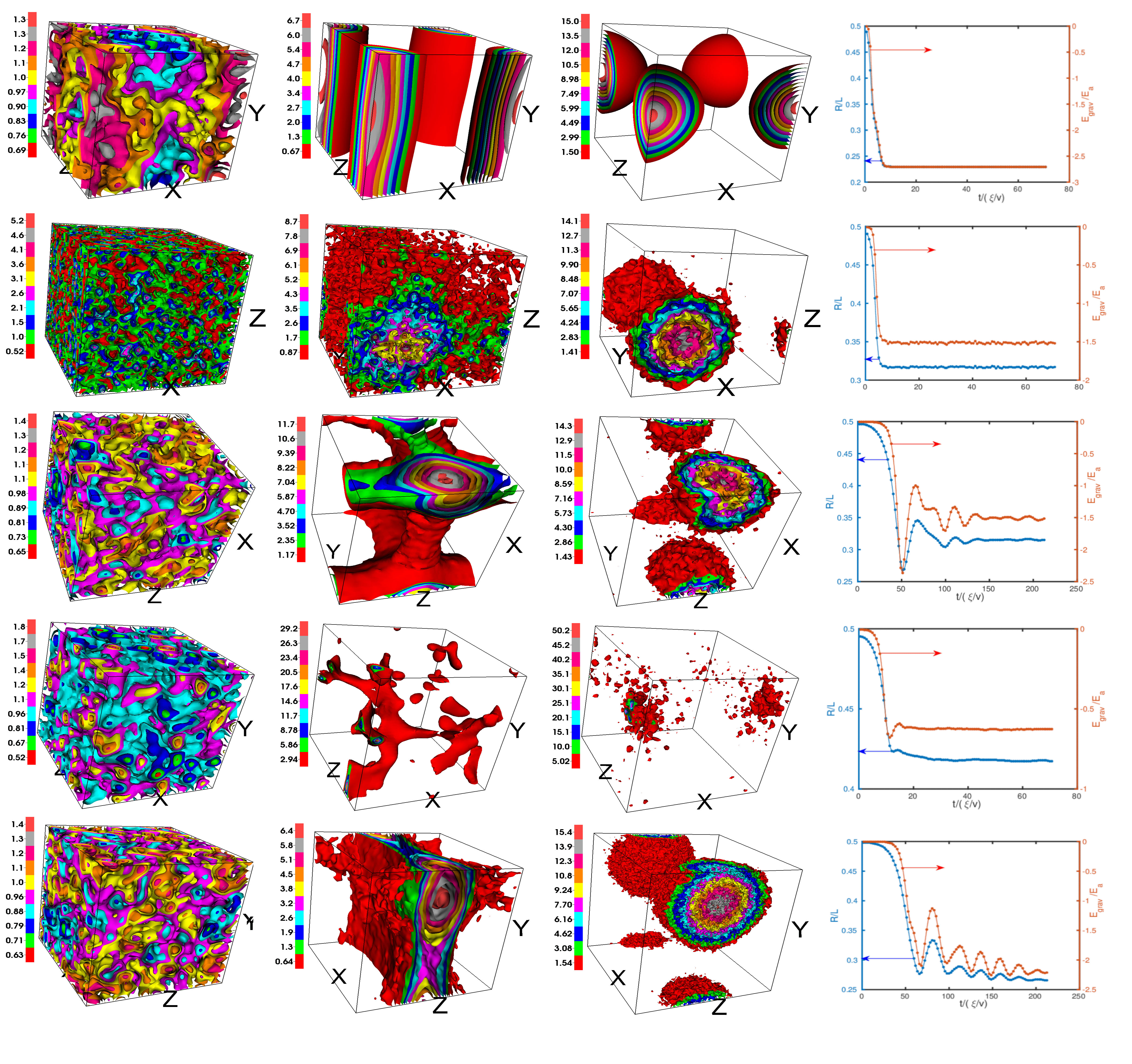
Figure 1: Columns $(1)-(3)$: Ten-level contour plots of ${\left|\psi({\bf x},t)\right|}^{2}$, at representative times: SGLPE ($T=0$) (top row, run $R1$); SGLPE (second row, run $R2$); GPPE (third row, run $R3$); GPPE (fourth row, run $R4$); and $256^{3}$ GPPE (fifth row, run $R5$) [the videos V1-V5 (Supplemental Material supplement ) show, respectively, the complete spatiotemporal evolution for these cases]. Column$(4)$: Plots of the scaled radius of gyration $\frac{R}{L}=\frac{1}{L}\sqrt{\frac{\int_{V}\rho(r)r^{2}d{\bf r}}{\int_{V}\rho(r)d{\bf r}}}$, (blue) and the scaled gravitational energy $E_{\rm grav}/E_{a}$ (red ) versus the scaled time $t/(\xi/v)$ for the different runs, where $E_{\rm a}=2^{5}\pi^{4}(G/g^{3})^{1/2}$.

A self-gravitating BEC is described by a complex wave function $\psi({\bf x},t)$; for weakly interacting bosons, the spatiotemporal evolution of $\psi({\bf x},t)$ is governed by the GPPE:

$$i\hbar\partial_{t}\psi = -\frac{\hbar^{2}}{2m}\nabla^{2}\psi+\left[G\Phi+g|\psi|^{2}\right]\psi,$$

$$\nabla^{2}\Phi = |\psi|^{2}-<|\psi|^{2}>,$$ (1)

where $m$ is the mass of the bosons, $n=|\psi|^{2}$ their number density, $\Phi$ is the gravitational potential field, $G=4\pi G_{\rm N}m^{2}$ ($G_{\rm N}$ is Newton’s constant), and $g=4\pi a\hbar^{2}/m$, with $a$ the $s$-wave scattering length. The subtraction of the mean density $\langle|\psi|^{2}\rangle$ can be justified either by taking into account the cosmological expansion Peebles ; falco2013 or by defining a Newtonian cosmological constant KIESSLING2003 . By linearizing Eq. (1) around the constant $|\psi|^{2}=n_{0}$, we obtain the dispersion relation $\omega(k)=\sqrt{-Gn_{0}/m+k^{2}gn_{0}/m+k^{4}(\hbar/2m)^{2}}$, which displays a low-$k$ Jeans instability, for wave numbers $k<k_{\rm J}=\sqrt{\frac{G}{g}}\left[\left(1+\sqrt{1+\frac{G\hbar^{2}}{mg^{2}n_{0}}}\right)/2\right]^{-1/2}$. In the absence of gravity ($G=0$), we identify the speed of sound $c=\sqrt{\frac{gn_{0}}{m}}$ and the coherence length $\xi=\sqrt{\frac{\hbar^{2}}{2g{n_{0}}m}}$. Units relevant to astrophysics are discussed in  Chavanis5 .

We solve the GPPE (1) by using the $3D$ Fourier pseudospectral method, with the $2/3$-rule for dealiasing Krstulovic11 ; vmrnjp13 ; Got-Ors : We expand the $2\pi$ periodic wave function as $\psi(x)=\sum_{{\bf k}\in\mathbb{Z}^{3}}\hat{\psi}_{\bf k}\exp(i{\bf k}\cdot{\bf x})$ and then we truncate it spectrally, by setting $\hat{\psi}_{\bf k}\equiv 0$ for $|{\bf k}|>k_{\rm max}$, with $k_{\rm max}=[{\cal N}/3]$, where $\cal{N}$ is the resolution and $[\cdot]$ denotes the integer part PhDTutorial ; Berloff14 . If we introduce the Galerkin projector $\mathcal{P}_{\rm G}$ [in Fourier space $\mathcal{P}_{\rm G}[\hat{\psi}_{\bf k}]=\theta(k_{\rm max}-|{\bf k}|)\hat{\psi}_{\bf k}$, with $\theta(\cdot)$ the Heaviside function], the Fourier-truncated GPPE becomes

$$i\hbar\frac{\partial\psi}{\partial t}=\mathcal{P}_{\rm G}[-\frac{\hbar^{2}}{2m}{\bf\nabla}^{2}\psi+\mathcal{P}_{\rm G}[(G{\bf\nabla}^{-2}+g)|\psi|^{2}]\psi].$$ (2)

Equation (2) conserves exactly the number of particles $N=\int d^{3}x|\psi|^{2}$ and the energy $E=E_{kq}+E_{int}+E_{G}$, where $E_{kq}=\frac{\hbar^{2}}{2m}\int d^{3}x|{\bf\nabla}\psi|^{2}$, $E_{int}=\frac{g}{2}\int d^{3}x[\mathcal{P}_{\rm G}|\psi|^{2}]^{2}$, and $E_{G}=E_{\rm grav}=\frac{G}{2}\int d^{3}x[\mathcal{P}_{\rm G}|\psi|^{2}]{\bf\nabla}^{-2}[\mathcal{P}_{\rm G}|\psi|^{2}]$. If we use the $2/3$-rule for dealiasing, then the momentum ${\bf P}=\frac{i\hbar}{2m}\int d^{3}x\left(\psi{\bf\nabla}\overline{\psi}-\overline{\psi}{\bf\nabla}\psi\right)$, where the over-bar denotes complex conjugation, is also conserved Krstulovic11 .

This spectral truncation generates a classical-field model that allows us to study finite-$T$ effects in the GPPE (Refs. Berloff14 ; Krstulovic11 ; vmrnjp13 for the GP case). We show that this spectrally truncated GPPE can describe dynamical effects and, at the same time, yield thermalized states, which we can obtain both by the thermalization of the long-time GPPE dynamics or directly, by using the SGLPE

$$\hbar\frac{\partial\psi}{\partial t} = \mathcal{P}_{\rm G}[\frac{\hbar^{2}}{2m}{\bf\nabla}^{2}\psi+\mu\psi-\mathcal{P}_{\rm G}[(G{\bf\nabla}^{-2}+g)|\psi|^{2}]\psi]$$ (3)

$$+\sqrt{\frac{2\hbar}{\beta}}\mathcal{P}_{\rm G}\left[\zeta({\bf x},t)\right],\hskip 8.53581pt$$

where the zero-mean, Gaussian white noise $\zeta({\bf x},t)$ has the variance $\langle\zeta({\bf x},t)\zeta^{*}({\bf x^{\prime}},t^{\prime})\rangle=\delta(t-t^{\prime})\delta({\bf x}-{\bf x^{\prime}})$, with $\beta=\frac{1}{k_{B}T}$ the inverse temperature; we tune the chemical potential $\mu$ at each time step to conserve the total number of particles $N$. The finite-$T$ SGLPE dynamics does not describe any physical evolution; but it converges more rapidly, than does the GPPE dynamics, toward a thermalized state (Refs. Berloff14 ; Krstulovic11 ; vmrnjp13 for the GP case). Clearly, the SGLPE leads to a state with a given temperature; but the GPPE yields a state with a given energy.

Our pseudospectral DNSs of the GPPE (1) and SGLPE (3) use a cubical computational domain that is $(2\pi)^{3}$ periodic; we normalise $\psi$ such that $N=(2\pi)^{3}$, and use units with $\hbar=1$ and $m=1$. We list the parameters for different runs in Tables 1 and 2.

$M_{\rm a}=\frac{\hbar}{\sqrt{G_{N}ma}}$	$\frac{M}{M_{\rm a}}=\frac{M\sqrt{Gg}}{4\pi\hbar^{2}}$
$R_{\rm a}=\sqrt{\frac{a\hbar^{2}}{m^{3}G_{N}}}$	$\frac{R}{R_{\rm a}}=\frac{R}{\sqrt{g/G}}$
$a_{\rm Q}=\frac{\hbar^{2}}{G_{N}M^{2}m}$	$\frac{a}{a_{\rm Q}}=\frac{M^{2}{Gg}}{(4\pi\hbar)^{2}}$
$R_{\rm Q}=\frac{\hbar^{2}}{G_{N}m^{2}M}$	$\frac{R}{R_{\rm Q}}=\frac{M{GR}}{4\pi\hbar^{2}}$

Table 1: Dimensionless variables: in the second column of the table we use quantities from the first column; $G_{\rm N}$ denotes Newton’s constant and $G=4\pi G_{\rm N}m^{2}$.

Run	R1	R2	R3	R4	R5
Type	SGLPE ($T=0$)	SGLPE	GPPE	GPPE	GPPE
$\cal{N}$	$64$	$64$	$64$	$64$	$256$
$g$	$50$	$50$	$50$	$5$	$50$
$G$	$105$	$105$	$105$	$550$	$105$

Table 2: This table shows the representative runs for which we give plots in Fig.$1$.

In columns $(1)-(3)$ of Fig. 1 we show ten-level contour plots of ${\left|\psi({\bf x},t)\right|}^{2}$ to illustrate, at representative times, the spatial organization of ${\left|\psi({\bf x},t)\right|}^{2}$ that we obatin via the SGLPE ($T=0$) (top row, run $R1$), the SGLPE (second row, run $R2$), and three GPPE runs (third row, run $R3$; fourth row, run $R4$; fifth row, run $R5$); the videos V1-V5 (Supplemental Material supplement ) show, respectively, the complete spatiotemporal evolution of ${\left|\psi({\bf x},t)\right|}^{2}$ for these five runs. In column $(4)$ of Fig. 1 we give, for these runs, plots of the scaled radius of gyration $R/L=\frac{1}{L}\sqrt{\frac{\int_{V}\rho(r)r^{2}d{\bf r}}{\int_{V}\rho(r)d{\bf r}}}$ (blue curves) and the scaled gravitational energy $E_{\rm grav}/E_{a}$ (red curves) versus the scaled time $t/(\xi/v)$, where $E_{\rm a}=2^{5}\pi^{4}(G/g^{3})^{1/2}$. If we tune $T$ in the SGLPE (3), it yields a statistically steady state whose properties (like $R/L$ and $E_{\rm grav}/E_{a}$) are close to their counterparts in the thermalized state of the GPPE (e.g., by comparing rows (2) and (3) in column(4) of Fig. 1 we see that the final state of the SGLPE has nearly the same energy and radius as the corresponding statistically steady GPPE state). Furthermore, convergence to this thermalized state is more rapid in the (canonical) SGLPE than in the (microcanonical) GPPE. To validate our DNSs, we have checked explicitly (Supplemental Material supplement ) that, at zero temperature, our results agree with those of the $T=0$ study of Refs. Chavanis1 ; Chavanis2 , which yield spherically symmetric ground states ( row $(1)$ of Fig. 1) with radius $R$ and $N$ bosons. Their ground-state energy can be approximated as $E(R)=\frac{\hbar^{2}N}{2mR^{2}}+\frac{gN^{2}}{2R^{3}}-\frac{GN^{2}}{2R}$ and the equilibrium radius follows from $dE/dR|_{R=R_{0}}=0$, whence $R_{0}=\frac{R_{\rm Q}}{4\pi}(1+\sqrt{1+48\pi^{2}(\frac{R_{\rm a}}{R_{\rm Q}}})^{2}$, where $R_{\rm Q}=\frac{\hbar^{2}}{G_{\rm N}m^{3}N}$ and $R_{\rm a}=\sqrt{\frac{a\hbar^{2}}{G_{\rm N}m^{3}}}$. The details of our extensive DNSs for the GPPE and the SGLPE are given in the Supplemental Material supplement (see, especially, Table I there). Figure 2(a) shows plots of of $R/R_{\rm Q}$ versus $a/a_{\rm Q}$ for three different values of $G$. In Fig. 2(b) we give plots of $M/M_{\rm a}$ versus $R/R_{\rm a}$, from our GPPE DNSs for three different values of $g$; the trends in these plots are markedly different than those at $T=0$ (see Fig.(1) in the Supplemental Material supplement ). In Fig. 2(c) we plot the scaled energies $E_{kq}/E_{a},\,E_{int}/E_{a},\,E_{\rm G}/E_{\rm a},$ and their total $E/E_{\rm a}$ versus the scaled temperature $k_{\rm B}T/E_{a}$ from our SGLPE DNSs; the jumps in these curves at $k_{\rm B}T/E_{\rm a}\simeq 3.25\times 10^{-5}$ suggest a first-order transition from a collapsed BEC to a tenuous, non-condensed assembly.

To confirm such a transition, we carry out an SGLPE hysteresis study, whose results are summarised in the plots in the panels of Fig. 3. The left panel of this figure shows $R/L$ versus $k_{\rm B}T/E_{\rm a}$; we obtain the red and green curves by, respectively, increasing and decreasing $k_{\rm B}T/E_{\rm a}$ (often referred to as heating and cooling runs in statistical mechanics). In these SGLPE runs, we use the final steady-state configuration for $\psi({\bf x})$, from the previous temperature, as the initial condition at the next temperature; clearly, there is significant hysteresis at the first-order transition from the - collapsed BEC to the non-collapsed state. In the right side panels of Fig. 3, we show ten-level contour plots of ${\left|\psi({\bf x})\right|}^{2}$ and the associated spectra ${\left|\psi(k)\right|}^{2}$ to illustrate, at representative points on heating and cooling curves in the hysteresis plot, the real-space density distribution and the $k-$space density spectra ($k_{\rm B}T/E_{\rm a}=2.7\times 10^{-5}$ and $k_{\rm B}T/E_{\rm a}=3.62\times 10^{-5}$ in the top panels A and B, respectively, and $k_{\rm B}T/E_{\rm a}=2.3\times{10^{-5}}$ and $k_{\rm B}T/E_{\rm a}=3.16\times 10^{-5}$ in the bottom panels C and D, respectively). From these density distributions and spectra, we conclude that our system undergoes a first-order transition from a collapsed BEC to a tenuous, non-condensed assembly. The panel of figures at the very bottom of Fig. 3 show that this first-order transition occurs at $g=0$ too. We expect that this also occurs when $g<0$, which is the appropriate parameter range for axion stars Chavanis4 ; Chavanis5 ; the $g<0$ case requires a quintic nonlinearity in Eq. 1 for stability; finite-temperature effects can be studied for this case by using the methods that we have described above (as we will show in future work).

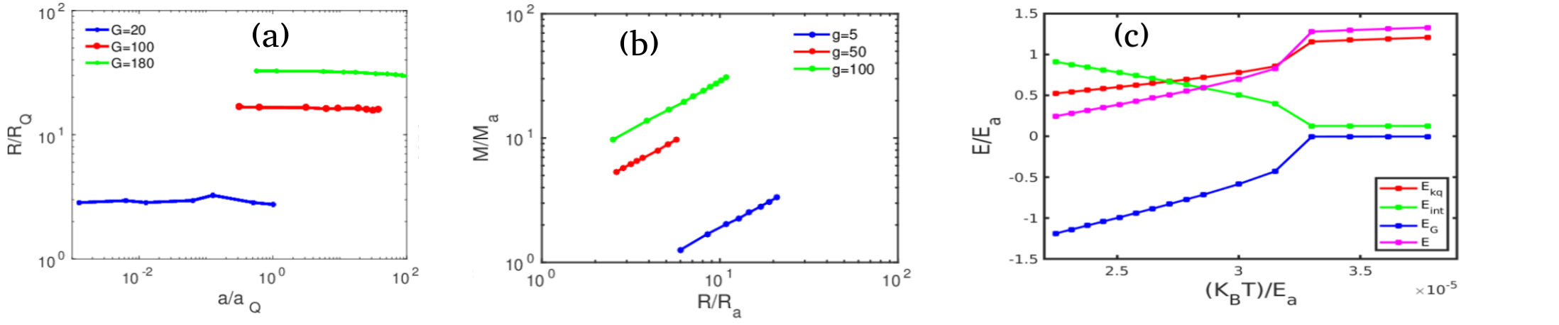
Figure 2: The plots of (a) the scaled radius of gyration $(R/R_{\rm Q})$ versus scaled scattering length $(a/a_{\rm Q})$ for the GPPE Runs A1-A30, (b) the scaled mass $(M/M_{\rm a})$ versus the scaled radius of gyration $R/R_{\rm a}$ for GPPE Runs B1-B30 on a log-log scale, (c) the scaled energy components ($E_{\rm kq}/E_{\rm a},E_{\rm int}/E_{\rm a},E_{\rm G}/E_{\rm a})$, and the total energy $(E/E_{\rm a})$ versus the scaled temperature $k_{\rm B}T/E_{\rm a}$.

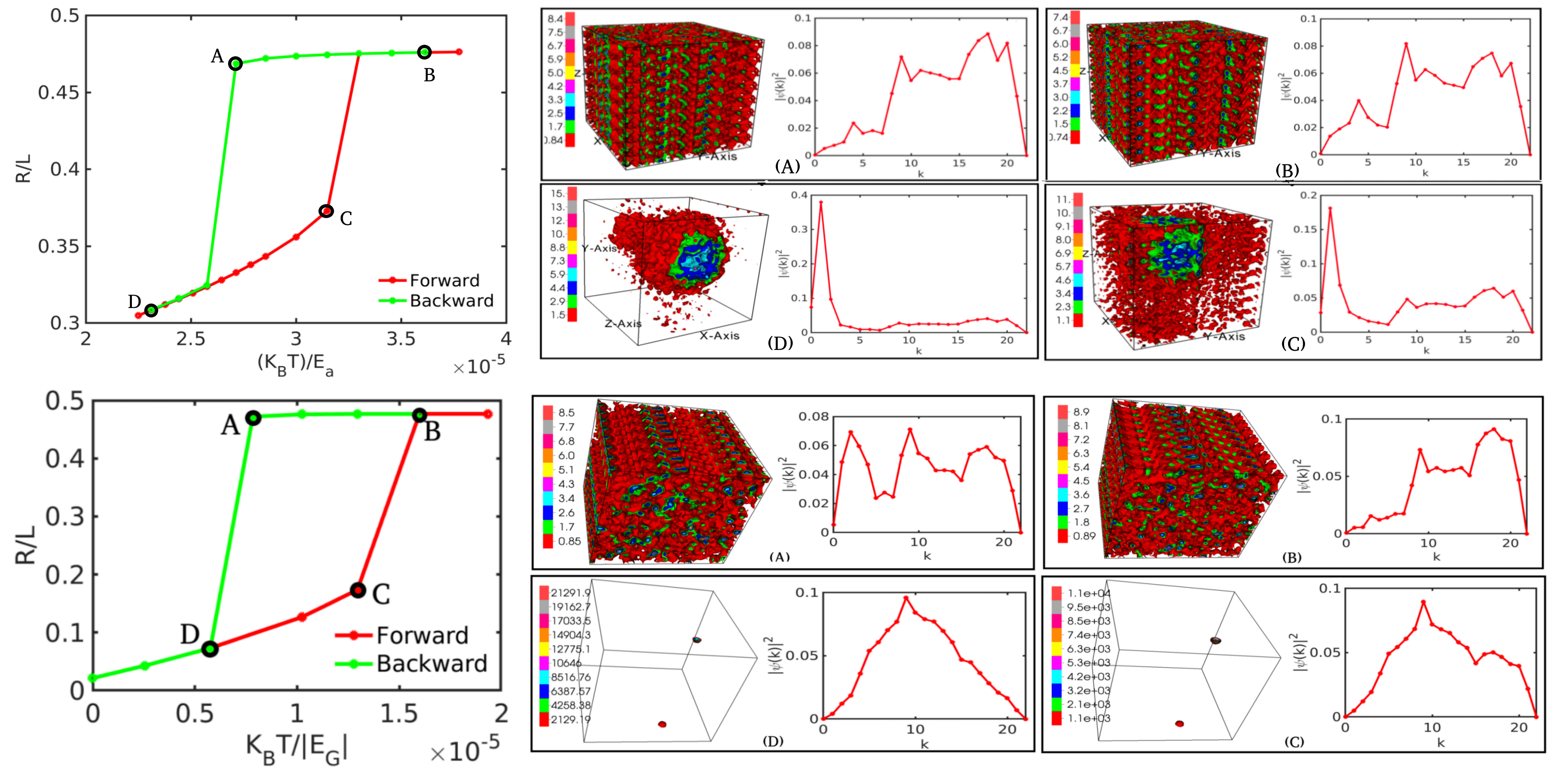
Figure 3: Top left panel: plots of the dimensionless radius ($R/L$) versus the dimensionless temperature ($k_{\rm B}T/E_{a}$), for heating (red) and cooling (green) runs showing a hysteresis loop. We show ten-level contour plots of ${\left|\psi({\bf x})\right|}^{2}$ and the associated spectra ${\left|\psi(k)\right|}^{2}$ to illustrate, at representative points on heating and cooling curves in the hysteresis plot, the real-space density distribution and the $k-$space density spectra ($k_{\rm B}T/E_{\rm a}=2.7\times 10^{-5}$ and $k_{\rm B}T/E_{\rm a}=3.62\times 10^{-5}$ in panels A and B of top panels, respectively, and $k_{\rm B}T/E_{\rm a}=2.3\times{10^{-5}}$ and $k_{\rm B}T/E_{\rm a}=3.16\times 10^{-5}$ in panels C and D of bottom panels, respectively). The analogs of these plots, for the case $g=0$, are shown in the panels at the very bottom. In the bottom left panel we use $|E_{G}|$ at $T=0$ to make the temperature dimensionless.

Do our Fourier-truncated GPPE yield only single collapsed objects? No. We now show, for the illustrative parameter values $g=20$, $G=1000$, and $128^{3}$ collocation points, that this GPPE can also yield long-lived states with temporal oscillations. In particular, by using an initial condition with two rotating spherical compact objects, the truncated GPPE dynamics yields a rotating binary system, which we depict at representative times in Fig. 4 and in the Video V6 in the Supplementary Material supplement (this also gives the initial data).

Our study goes well beyond earlier studies  harkofinite ; schivecosmic that employ the Thomas-Fermi approximation and include finite-temperature effects at the level of a non-interacting Bose gas (with $g=0$). We have shown that the truncated GPPE can be used effectively to study the graviational collapse of an assembly of weakly interacting bosons at finite temperature. Our study of this collapse shows that there is a clear, thermally driven first-order transition from a non-condensed bosonic gas, at high $T$, to a condensed BEC phase at low $T$; this transition should be contrasted with the continuous BEC transition in the weakly interacting Bose gas, which is described by the GPE, in the absence of gravitation. Furthermore, we have shown that gravitationally bound, rotating binary objects can be obtained in our GPPE simulations. Therefore, our work opens up the possibility of carrying out detailed finite-temperature studies of self-gravitating bosonic systems, which are potentially relevant for studies of dark-matter candidates like boson stars and axions.

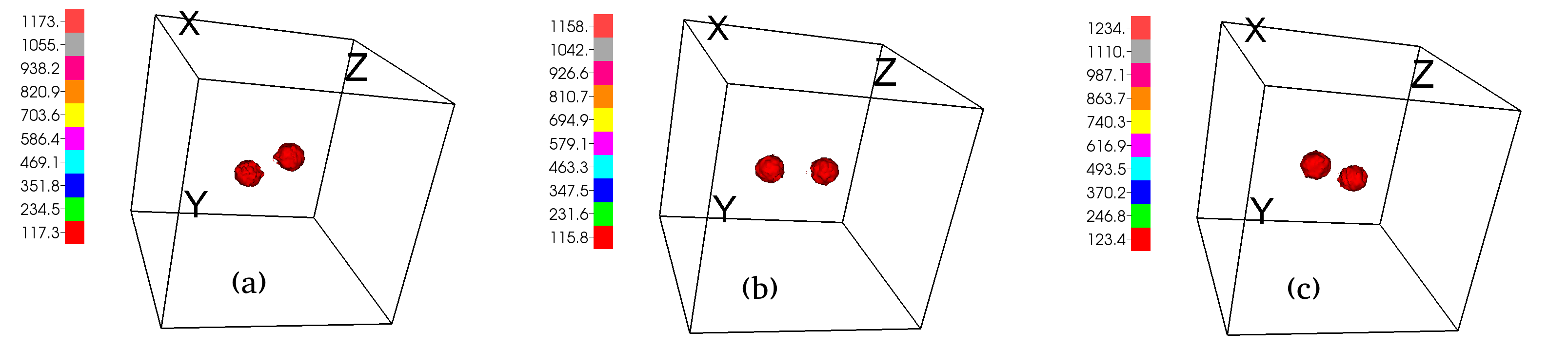
Figure 4: Ten-level contour plots of the $|\psi({\bf x},t)|^{2}$ (a) at $t=0.018$, (b) at $t=0.025$, and (c) at $t=0.03$, for the initial condition for $\psi({\bf x},t)$ given in Eq.(1) of the Supplementary Material supplement , showing rotating binary system (see video V6 in supplemental material).

Acknowledgements: We thank DST, CSIR (India), and the Indo French Center for Applied Mathematics (IFCAM) for their support.

References

- (1) D. O’Dell, S. Giovanazzi, G. Kurizki, and V. M. Akulin, Phys. Rev. Lett. 84, 5687 (2000).
- (2) R. Ruffini and S. Bonazzola, Phys. Rev. 187, 1767 (1969).
- (3) G. Ingrosso, D. Grasso, and R. Ruffini, Astron. Astro- phys. 248, 481 (1991).
- (4) P. Jetzer, Physics Reports 220, 163 (1992).
- (5) W. Hu, R. Barkana, and A. Gruzinov, Phys. Rev. Lett. 85, 1158 (2000).
- (6) H. Abdallah et al., Phys. Rev. Lett. 120, 201101 (2018).
- (7) C. Kachulis et al., Phys. Rev. Lett. 120, 221301v(2018).
- (8) https://physics.aps.org/articles/v11/48?utm_campaign=weekly&utm_medium=email&utm_source=emailalert
- (9) M. Lawson et al., Phys. Rev. Lett. 123, 141802 (2019).
- (10) P.-H. Chavanis, Phys. Rev. D 84, 043531 (2011).
- (11) P.-H. Chavanis and L. Delfini, Phys. Rev. D 84, 043532 (2011).
- (12) P.-H. Chavanis, Phy. Rev. D 94, 083007 (2016).
- (13) P.-H. Chavanis, Phys. Rev. D 98, 023009 (2018).
- (14) P.-H. Chavanis, Quantum Aspects of Black Holes, eds. X. Calmet et al, (Springer, 2015), pp. .
- (15) N. P. Proukakis and B. Jackson, Journal of Physics B: Atomic, Molecular and Optical Physics 41, 203002 (2008).
- (16) N. G. Berloff, M. Brachet, and N. P. Proukakis, Proc. Natl. Acad. Sci. U.S.A. 111, 4675 (2014).
- (17) G. Krstulovic and M. Brachet, Phys. Rev. E 83, 066311 (2011).
- (18) V. Shukla, M. Brachet, and R. Pandit, New J. Phys. 15, 113025 (2013).
- (19) Supplemental Material (2019).
- (20) P. Peebles, The large-scale structure of the universe, 2011 (Princeton University Press, Princeton, NJ, 1980).
- (21) M. Falco, S. H. Hansen, R. Wojtak, and G. A. Mamon, Mon. Not. R. Astron. Soc. 431, L6 (2013).
- (22) M. K.-H. Kiessling, Advances in Applied Mathematics 31, 132 (2003).
- (23) D. Gottlieb, and S. A. Orszag, Numerical Analysis of Spectral Methods (SIAM, Philadelphia, 1977).
- (24) T. Harko, and J.M. Madarassy, J. Cosmol. Astropart. Phys. 01 (2012) 025.
- (25) H-Y. Schive, T. Chiueh, and T. Broadhurst, Nat. Phys. 10, 496 (2014) .