Methods for comparing uncertainty quantifications for material property predictions

Abstract

Data science and informatics tools have been proliferating recently within the computational materials science and catalysis fields. This proliferation has spurned the creation of various frameworks for automated materials screening, discovery, and design. Underpinning these frameworks are surrogate models with uncertainty estimates on their predictions. These uncertainty estimates are instrumental for determining which materials to screen next, but the computational catalysis field does not yet have a standard procedure for judging the quality of such uncertainty estimates. Here we present a suite of figures and performance metrics derived from the machine learning community that can be used to judge the quality of such uncertainty estimates. This suite probes the accuracy, calibration, and sharpness of a model quantitatively. We then show a case study where we judge various methods for predicting density-functional-theory-calculated adsorption energies. Of the methods studied here, we find that the best performer is a model where a convolutional neural network is used to supply features to a Gaussian process regressor, which then makes predictions of adsorption energies along with corresponding uncertainty estimates.

These authors contributed equally to this work These authors contributed equally to this work

1 Introduction

The fields of catalysis and materials science are burgeoning with methods to screen, design, and understand materials.^{1, 2, 3, 4} This research has spurned the creation of Machine Learning (ML) models to predict various material properties. Unfortunately, the design spaces for these models are sometimes too large and intractable to sample completely. These under-sampling issues can limit the training data and therefore the predictive power of the models. It would be helpful to have an uncertainty quantification (UQ) for a model so that we know when to trust the predictions and when not to. More specifically: UQ would enable various online, active frameworks for materials discovery and design (e.g., active learning,⁵ online active learning,⁶ Bayesian optimization,⁷ active search,⁸ or goal oriented design of experiments⁹).

Such active frameworks have already been used successfully in the field of catalysis and materials informatics. For example: Peterson ¹⁰ has used a neural network to perform online active learning of nudged elastic band (NEB) calculations, reducing the number of force calls by an order of magnitude. Torres et al. ¹¹ have also used online active learning to accelerate NEB calculations, but they used a Gaussian Process (GP) model instead of a neural network. Jinnouchi et al. ¹² have used online active learning to accelerate molecular dynamics simulations. These methods are all underpinned by models with UQ, which have garnered increasing attention.^{13, 14}

The goal of UQ is to quantify accurately the likelihood of outcomes associated with a predicted quantity. For example, given an input for which we wish to make a prediction, a predictive UQ method might return a confidence interval that aims to capture the true outcome a specified percentage of the time or might return a probability distribution over possible outcomes. Performance metrics for predictive UQ methods aim to assess how well a given quantification of the probabilities of potential true outcomes adheres to a set of observations of these outcomes. Some of the performance metrics for predictive UQ are agnostic to prediction performance—they provide an assessment of the uncertainty independent of the predictive accuracy (i.e. a method can predict badly, but could still accurately quantify its own uncertainty).

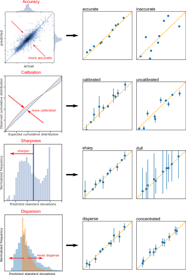
We have seen few^{15, 16} comparisons of different methods for UQ within the field of catalysis and materials informatics. Here we examine a protocol^{17, 18} for comparing the performance of different modeling and UQ methods (Figure 1). We then illustrate the protocol on a case study where we compare various models’ abilities to predict Density Functional Theory (DFT) calculated adsorption energies. We also offer anecdotal insights from our case study. We acknowledge that such insights may not be transferable to other applications, but we find value in sharing them so that others can build their own intuition.

Figure 1: Overview of proposed procedure for judging the quality of models with uncertainty estimates. First and foremost, the models should be accurate. Second, the models should be “calibrated”, which means that their uncertainty estimates should be comparable with their residuals. Third, the models should be “sharp”, which means that their uncertainty estimates should be low. Lastly, the models should be “disperse”, which means that the distribution of the uncertainty estimates should be wide. This study demonstrates how to visualize and quantify these characteristics so that different methods of UQ can be compared objectively.

2 Methods

2.1 Dataset information

All regressions in this paper were performed using a dataset of 47,279 DFT calculated adsorption energies created with the Generalized Adsorption Simulator for Python (GASpy) ^{19, 20}. Within this dataset, there were 52 different elements within the 1,952 bulk structures used as bases for the adsorption surfaces. The 61 bulk structures that contained one element encompassed 5,844 of the adsorption calculations; the 1,057 bulk structures that contained two elements encompassed 31,651 of the calculations; the 774 bulk structures that contained three elements encompassed 9,139 of the calculations; and the 60 bulk structures that contained four or five elements encompassed 645 of the calculations. The dataset also comprised 9,102 symmetrically distinct surfaces and 29,843 distinct coordination environments (as defined by the surface and the adsorbate neighbors). Lastly, the dataset comprised 21,269 H adsorption energies; 18,437 CO adsorption energies; 3,464 OH adsorption energies; 2,515 O adsorption energies; and 1,594 N adsorption energies.

GASpy performed all DFT calculations using the Vienna Ab-initio Simulation Package (VASP) ^{21, 22, 23, 24} version 5.4 implemented in the Atomic Simulation Environment (ASE) ²⁵. The revised Perdew-Burke-Ernzerhof (rPBE) functionals²⁶ were used along with VASP’s pseudopotentials, and no spin magnetism or dispersion corrections were used. Bulk relaxations were performed with a $10\times 10\times 10$ k-point grid and a 500 electron volts (eV) cutoff, and only isotropic relaxation were allowed during this bulk relaxation. Slab relaxations were performed with k-point grids of $4\times 4\times 1$ and a 350 eV cutoff. Slabs were replicated in the X/Y directions so that each cell was at least 4.5 Å wide, which reduces adsorbate self-interaction. Slabs were also replicated in the Z direction until they were at least 7 Å thick, and at least 20 Å of vacuum was included in between slabs. The bottom layers of each slab were fixed and defined as those atoms more than 3 Å from the top of the surface in the scaled Z direction.

To split the data into train/validate/test sets, we enumerated all adsorption energies on monometallic slabs and added them to the training set manually. We did this because some of the regression methods in this paper use a featurization that contains our monometallic adsorption energy data¹⁹, and so having the monometallic adsorption energies pre-allocated in the training set prevented any information leakage between the training set and validation/test sets. After this allocation, we performed a 64/14/20 train/validate/test split that was stratified²⁷ by adsorbate. We then used the validation set’s results to tune various hyperparameters manually. After tuning, we calculated the test set results and present them in this paper exclusively. Note that the test results were obtained using models that were trained only using the training set, not the validation set. This is acceptable because we only seek to compare methods here, not to optimize them.

Note that random splits such as this may yield overly optimistic model results. If a model created with the training set is meant to make extrapolative predictions in feature domains outside of the training set, then it may be appropriate to use a train/validate/test split using k-means clustering²⁸ rather than random splitting. If the model is meant to be used in an online and iterative fashion, then it may be appropriate to use a time-series split²⁹. If the model is meant to be used to interpolate within a given feature space, then the basic random split may be appropriate. We chose to use a basic random split in this work to simplify the results for illustrative purposes. Future work for different applications should use splitting methods that align with the intended use of the models to be generated.

2.2 Regression methods

We explore various methods that aim to quantify the uncertainty for regression procedures where the predicted quantity is a continuous variable. To standardize the assessment of performance, we ensure that each UQ method returns predictive uncertainty results in a consistent format: a distribution over possible outcomes of the predicted quantity for any specified input point. This result format allows us to compute all the predictive uncertainty performance metrics which we introduce in subsequent sections. Figure 2 illustrates all of the methods we investigate in this study, and we describe each method in detail below.

Figure 2: Overview of the various UQ methods we investigated in this study. $\Delta E$ represents DFT-calculated adsorption energies; $\Delta\hat{E}$ represents ML-predicted adsorption energies; $UQ$ represents ML-predicted uncertainty quantifications; $\mu$ represents the mean of a sample of points; $\sigma$ represents the standard deviation of a sample of points; $\epsilon$ represents the residuals between DFT and ML; and $\hat{\epsilon}$ represents the residuals between ML-predicted $\epsilon$ and the actual $\epsilon$.

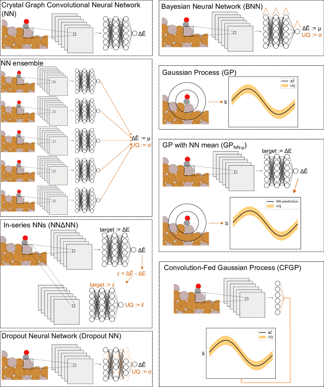
NN: To establish a baseline for predictive accuracy, we re-trained a previously reported crystal graph convolutional Neural Network (NN) ^{30, 31} on this study’s training set. This NN model projects a three-dimensional atomic structure into a graph, which is then fed into convolutional layers to extract local atomic information for predicting global target properties. In this case, we predict DFT-calculated adsorption energies, $\Delta$E. The graph consists of nodes representing atoms and edges representing distances between atoms. The NN updates the node features using the local information extracted in the convolutional layers, then hidden layers in the NN maps the node features to the adsorption energies. Reference Back et al. ³¹ for additional details.

NN Ensemble: We created an ensemble of NN s by 5-fold subsampling the training data and then training individual NN models on the 5 folds. Each individual NN model’s architecture is identical to the base NN architecture outlined previously. The only differences are their training sets and their individually randomized initial weights. For the final prediction of the ensemble we computed the mean of the set of models’ predictions, and for the ensemble’s estimate of uncertainty we computed the standard deviation of the set of predictions.

BNN: The aim of Bayesian Neural Network (BNN) is to determine the posterior distribution of model parameters rather than a single optimal value of the parameters. In practice, inferring true posterior distributions is very difficult and even infeasible in most cases. Thus, we approximate the model posterior to be as close as possible to the true posterior. The same NN architecture was used, but we converted the NN into BNN by assigning posterior distributions to all model parameters in the hidden layers in the NN model. The BNN then approximated the true posterior distributions using variational inference so that it could use the approximated posterior to predict the adsorption energies. We sampled the model parameters 20 times from the approximated posterior distributions, and used the mean of these predictions as the final prediction and the standard deviation of these predictions as the estimation of uncertainty. We implemented the BNN and performed variational inference using Pyro.³²

Dropout NN: Dropout Neural Networks (Dropout NN) have been shown to approximate Bayesian models.³³ We created a Dropout NN by first replicating the exact architecture used to create the convolutional NN outlined previously. Then we enforced a random dropout rate of 30% in the dense hidden layers that followed the convolutional layers. The nodes were randomly dropped out during both training and prediction. To make predictions, we sampled the Dropout NN 20 times. The mean of the predictions was used as the final prediction of the Dropout NN, and the standard deviation of the predictions was used as the estimation of uncertainty.

NN$\Delta$NN: Suppose we have trained a NN. We may aim to empirically fit an additional mapping that predicts the error of the first NN. Here we show in-series NNs (NN$\Delta$NN), which trains a secondary NN to predict the residuals of the initial NN. When training the first NN, we hold out 10% of the training data. Afterwards, we use the residuals of the initial NN on the held-out portion as training data for the second NN. After the secondary training, this second NN can predict residuals for the first NN on some new set of input data. The predictions of the second NN can then be used as uncertainty estimates. Note that both the NN s included within the NN$\Delta$NN were constructed using the same convolutional architecture outlined previously.

GP: GP s are one of the most common regression methods for producing UQ s, and so we use them here as a baseline. We fit a standard GP using the same exact features that we used in previous work.¹⁹ These features are defined by the elements coordinated with the adsorbate and by the elements of its next-nearest neighbors. Specifically: We use the atomic numbers of these elements, their Pauling electronegativity, a count of the number of atoms of each element near the adsorbate, and the median adsorption energy between the adsorbate and the elements. To ensure that these features interacted well with the GP’s kernel, we normalized each of the features to have a mean of zero and standard deviation of one. Reference Tran and Ulissi ¹⁹ for additional details. To define the GP, we assumed a constant mean and used a Matern covariance kernel. We trained the length scale of the Matern kernel using the Maximum Likelihood Estimation (MLE) method. All GP training and predictions were done with GPU acceleration as implemented in GPyTorch.³⁴.

GP_NN-μ: GP s are Bayesian models in which a prior distribution is first specified and then updated given observations to yield a posterior distribution. The mean of this posterior distribution is used for regression, and the covariance matrix is used for UQ. Typically, in lieu of any additional prior knowledge, practitioners will take the prior distribution to have zero-mean. However, we could instead supply an alternative curve for the prior mean, and then perform the usual Bayesian updates to compute the posterior of this GP given observations. Here, for the GP prior mean, we supply the prediction given by a single pre-trained NN. We call this method GP with NN mean (GP_NN-μ). For the input features of this GP, we used the same exact features we used for the plain GP—i.e., the vector of atomic numbers, electronegativity, etc. For the covariance kernel of this GP, we used a Matern kernel where we fit the kernel hyperparameters using MLE. All GP training and predictions were done with GPU acceleration as implemented in GPyTorch.³⁴.

CFGP: A limitation of using this formulation of a GP with NN-predicted mean is that it requires the use of hand-crafted features for the GP. This requirement reduces the transferability of the method to other applications where such features may not be readily available. To address this, we formulated a different method where we first train a NN (as described previously) to predict adsorption energies and then fix the network’s weights. Then we use the 46 pooled outputs of the convolutional layers of the network as features in a new GP. The GP would then be trained to use these features to produce both mean and uncertainty predictions on the adsorption energies. We call this a Convolution-Fed Gaussian Process (CFGP). Note that we normalized the 46 convolution outputs of the NN so that each output would have a mean of zero and a standard deviation of one across the training set. To define the GP, we assumed a constant mean and used a Matern covariance kernel. We trained the length scale of the Matern kernel using the MLE method. All GP training and predictions were done with GPU acceleration as implemented in GPyTorch.³⁴.

2.3 Performance metrics

We used five different metrics to quantify the accuracy of the various models: Median Absolute Error (MDAE), Root Mean Squared Error (RMSE), Mean Absolute Error (MAE), Mean Absolute Relative Percent Difference (MARPD), and R² correlation coefficient (R²). We used MDAE because is insensitive to outliers and is therefore a good measure of accuracy for the majority of the data. We used RMSE because it is sensitive to outliers and is therefore a good measure of worst-case accuracy. We used MAE because it lies between MDAE and RMSE in terms of sensitivity to outliers. We used MARPD and R² because they provide normalized measures of accuracy that may be more interpretable for those unfamiliar with adsorption energy measurements in eV. MARPD values were calculated with Equation 1:

$$MARPD=\frac{1}{N}\sum_{n=1}^{N}\mathinner{\!\left\lvert 100\cdot\frac{\hat{x}_{n}-x_{n}}{\mathinner{\!\left\lvert\hat{x}_{n}\right\rvert}+\mathinner{\!\left\lvert x_{n}\right\rvert}}\right\rvert}$$ (1)

where $n$ is the index of a data point, $N$ is the total number of data points, $x_{n}$ is the true value of the data point, and $\hat{x}_{n}$ is the model’s estimate of $x_{n}$. In this case, $x_{n}$ is a DFT-calculated adsorption energy and $\hat{x}_{n}$ is the surrogate-model-calculated adsorption energy. The ensemble of these metrics provide a more robust view of accuracy than any one metric can provide alone.

To assess the calibration (or “honesty”) of these models’ UQ s, we created calibration curves. A calibration curve “displays the true frequency of points in each interval relative to the predicted fraction of points in that interval”, as outlined by Kuleshov et al. ¹⁷. In other words: We used the standard deviation predictions to create Gaussian random variables for each test point and then tested how well the residuals followed their respective Gaussian random variables. Thus “well-calibrated” models had residuals that created Gaussian distributions whose standard deviations were close to the model’s predicted standard deviations. We discuss calibration curves in more detail in the Results section alongside specific examples. We also calculated the calibration errors¹⁷ of our models, which is a quantitative measure of calibration.

As Kuleshov et al. ¹⁷ also pointed out, well-calibrated models are necessary but not sufficient for useful UQ s. For example: A well-calibrated model could still have large uncertainty estimates, which are inherently less useful than well-calibrated and small uncertainty estimates. This idea of having small uncertainty estimates is called “sharpness”, and Kuleshov et al. ¹⁷ define it with Equation 2:

$$sha=\frac{1}{N}\sum_{n=1}^{N}var(F_{n})$$ (2)

where $var(F_{n})$ is the variance of the random variable whose cumulative distribution function is $F$ at point $n$. This is akin to the average variance of the uncertainty estimates on the test set. Here we propose and use a new formulation (Equation 3) where we add a square root operation. This operation gives the sharpness the same units as the predictions, which provides us with a more intuitive reference. In other words: Sharpness is akin to the average of the ML-predicted standard deviations.

$$sha=\sqrt{\frac{1}{N}\sum_{n=1}^{N}var(F_{n})}$$ (3)

Another consideration is the dispersion of the uncertainty estimates. If a model predicts a constant value for uncertainty, it may still be able to perform well with regards to calibration or sharpness. Constant values for uncertainty are likely to fail when models are used to make predictions outside the bounds of the training data. One way to address this issue is to calculate the coefficient of variation (C_v) ¹⁸. See Equation 4:

$$C_{v}=\frac{\sqrt{\frac{\sum_{n=1}^{N}(\sigma_{n}-\mu_{\sigma})^{2}}{N-1}}}{\mu_{\sigma}}$$ (4)

where $\sigma_{n}$ is the predicted standard deviation of point $n$, $\mu_{\sigma}$ is the average value of $\sigma_{n}$, and $N$ is the total number of test points. Low values of C_v indicate a narrow dispersion of uncertainty estimates, which may suggest poor performance in out-of-domain predictions. Thus a higher C_v may indicate more robust uncertainty estimates. But as Scalia et al. ¹⁶ point out, the optimal dispersion is a function of the validation/test data distribution. Therefore, C_v should be used as a secondary screening metric rather than a primary performance metric.

We also assessed the performance of each predictive uncertainty method by comparing their negative log-likelihood (NLL) values the test set. For each test point, we established a Gaussian probability distribution using the mean and uncertainty predictions of each UQ model. Then we calculated the conditional probability of observing the true value of the test point given the probability distribution created from the UQ; this is the likelihood of one test point. We then calculated the product of all the likelihoods of all test points, which yielded the total test likelihood. It follows that better UQ methods yield higher total likelihood values. Equivalently, we could calculate the natural logarithms of each likelihood, sum them, and then take the negative of this value; this is NLL. Equation 5 shows how we calculated NLL:

$$NLL=-\sum_{i=1}^{n}\ln{P(y_{i}|N(\hat{y_{i}},\hat{\sigma_{i}}^{2}))}$$ (5)

where $y_{i}$ is the true value of a test point, $\hat{y}_{i}$ is a model’s predicted mean value at that test point, $\hat{\sigma_{i}}^{2}$ is the model’s predicted variance at that test point, $n$ is the set of all test points, and $N(x,y)$ is a normal distribution with mean $x$ and variance $y$. Note how the NLL value depends on the size and location of the test set. This means that the absolute value of NLL changes from application to application, and so a “good” NLL value must be contextualized within a particular test set. Within a test set, a lower NLL value indicates a better fit. We also note that we assumed Gaussian distributions for our UQ methods’ predictions. This assumption does not necessarily need to be applied, meaning that the normal distribution in Equation 5 may be replaced with any other appropriate distribution.

We use NLL because it provides an overall assessment that is influenced by both the predictive accuracy of a method as well as the quality of its UQ. Previous work ^{35, 36} has shown the NLL to be a strictly proper scoring rule, which intuitively means that it provides a fair quantitative assessment (or score) for the performance of the UQ method, and that it can be decomposed into terms that relate to both calibration and sharpness. NLL is also a popular performance metric that has been used to quantify uncertainty in a variety of prior work ³⁷ and provides an additional single score for UQ methods.

3 Results

3.1 Illustrative examples

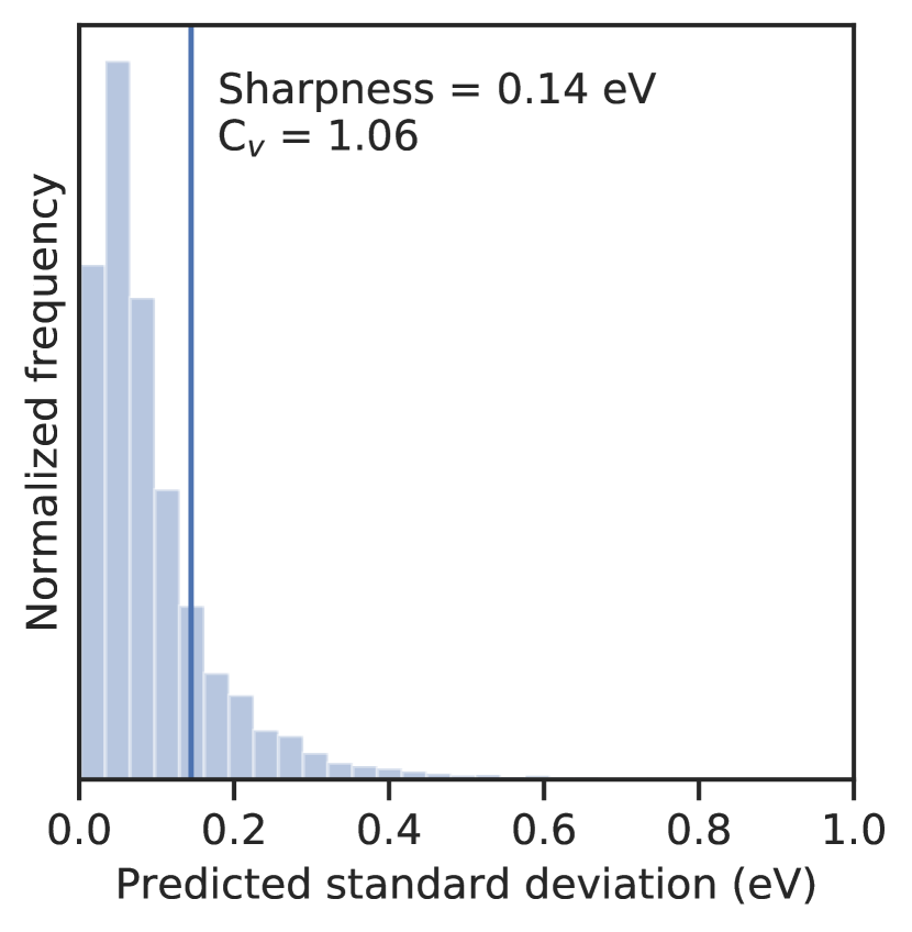
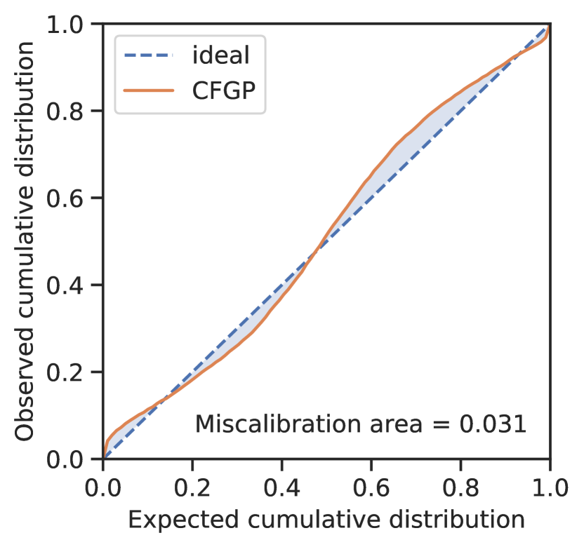
Let us first discuss the results of our NN ensemble for illustrative purposes. Figure 3 contains a parity plot, calibration curve, and predicted-uncertainty distribution of our NN ensemble model. The parity plot shows the accuracy of the model; the calibration curve shows the honesty of the model’s uncertainty predictions; and the uncertainty distribution shows the sharpness of the model’s uncertainty predictions. Accurate models have parity plots whose points tend to fall near the diagonal parity line. Calibrated models have calibration curves that approach the ideal diagonal line. Sharp models have uncertainty distributions that tend towards zero. Note that sharpness should not be won at the cost of calibration.

(a) parity plot

(b) calibration curve

(c) uncertainty distribution

Figure 3: Results of the NN ensemble. Each figure here was created with the test set of 8,289 points.

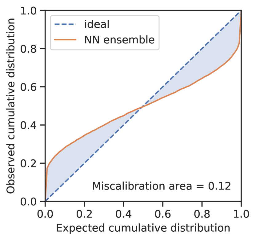
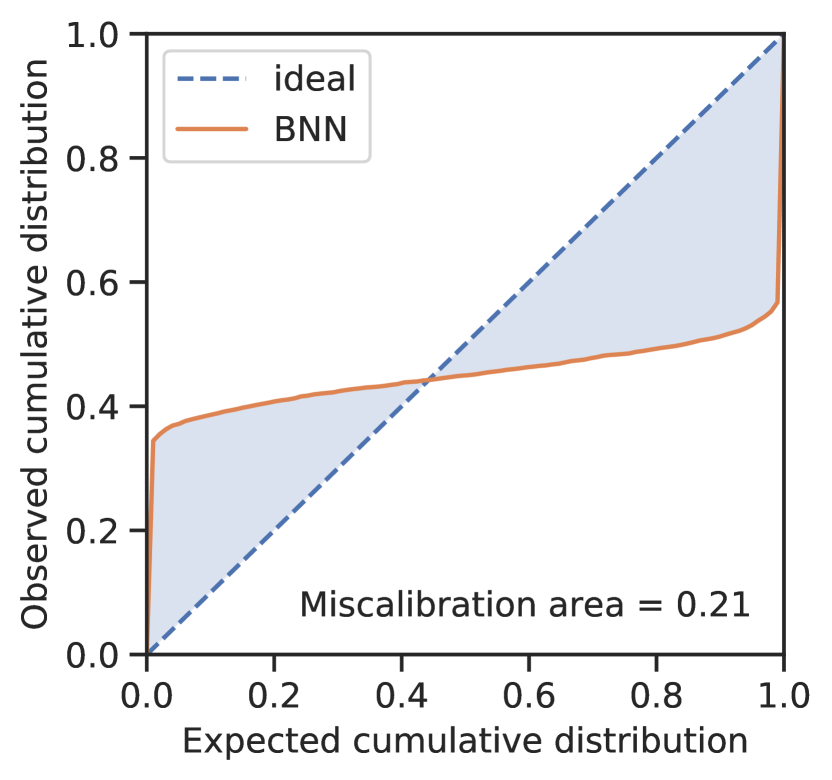
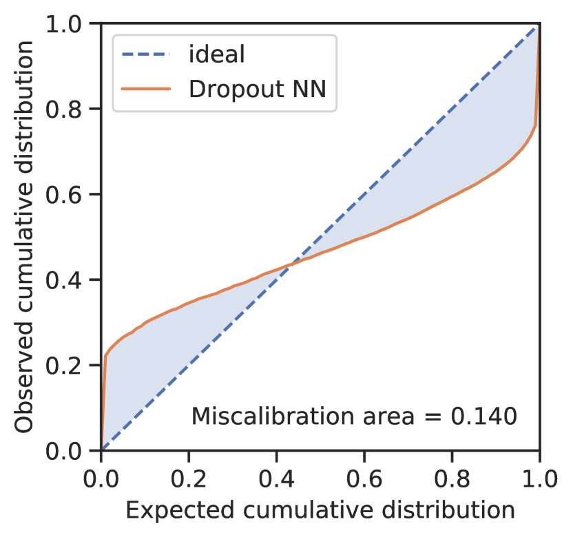
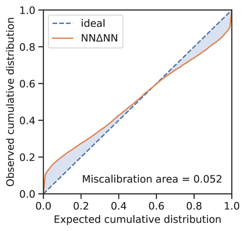
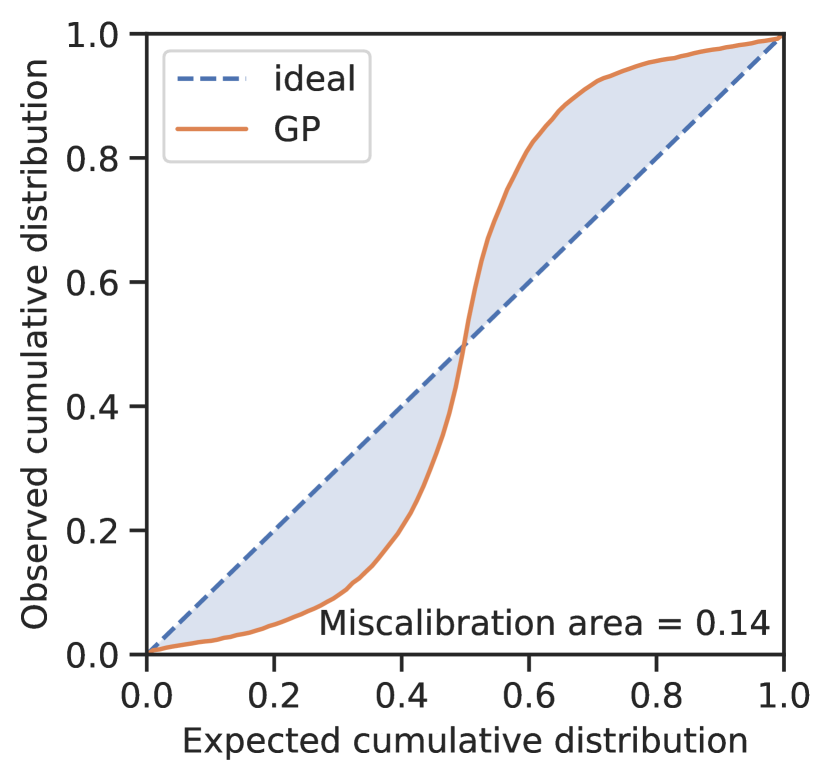
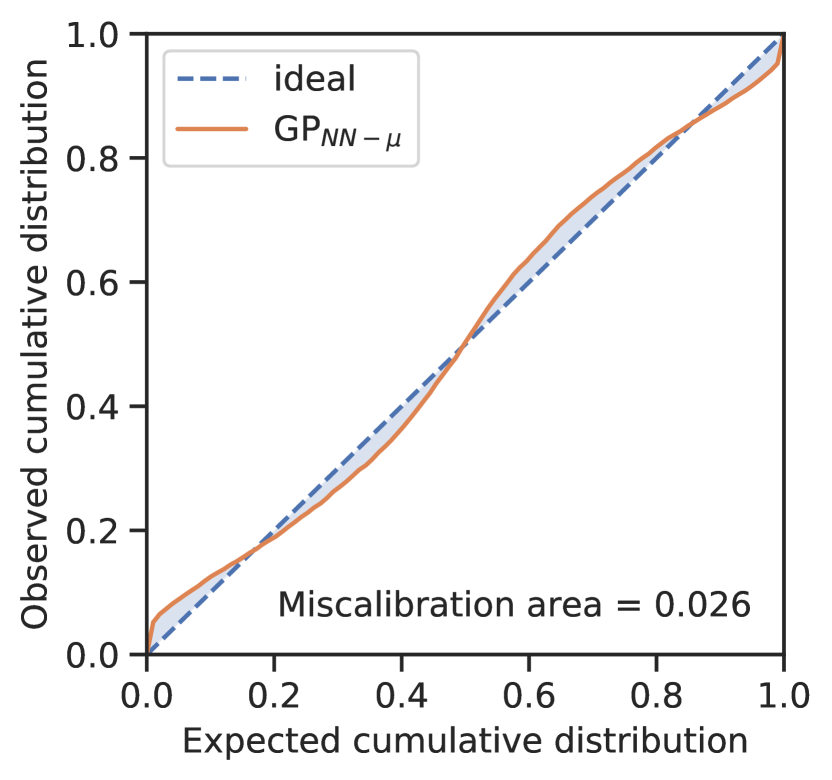
The calibration curve was created by first establishing Gaussian random variables for each test point where the means were the model’s predictions and the variances were the model’s predicted variances. The test residuals could then be compared against their respective random variables. For simplification purposes, we divided each of the test residuals by their corresponding standard deviations so that we could test all residuals against the same unit Gaussian distribution. Thus if the normalized test residuals followed a unit Gaussian distribution, then the model’s uncertainty predictions could be considered well-calibrated. We tested this by calculating the theoretical cumulative distribution of points within the intervals $(-\infty,x]\mkern 9.0mu\forall\mkern 9.0mux\in(-\infty,\infty)$ and then compared it against the observed cumulative distributions. A plot of the observed cumulative distributions against the theoretical cumulative distributions is called a calibration curve. A perfectly calibrated model would have normalized residuals that are Gaussian, which would yield a diagonal calibration line. Therefore, models’ calibration could be qualified by the closeness of their calibration curves to this ideal, diagonal curve. We quantified this closeness by calculating the area between the calibration curve and the ideal diagonal. We call this the miscalibration area, and smaller values indicate better calibration. We also calculated the calibration error,¹⁷ which is the mean square difference between the expected cumulative distributions and observed cumulative distributions.

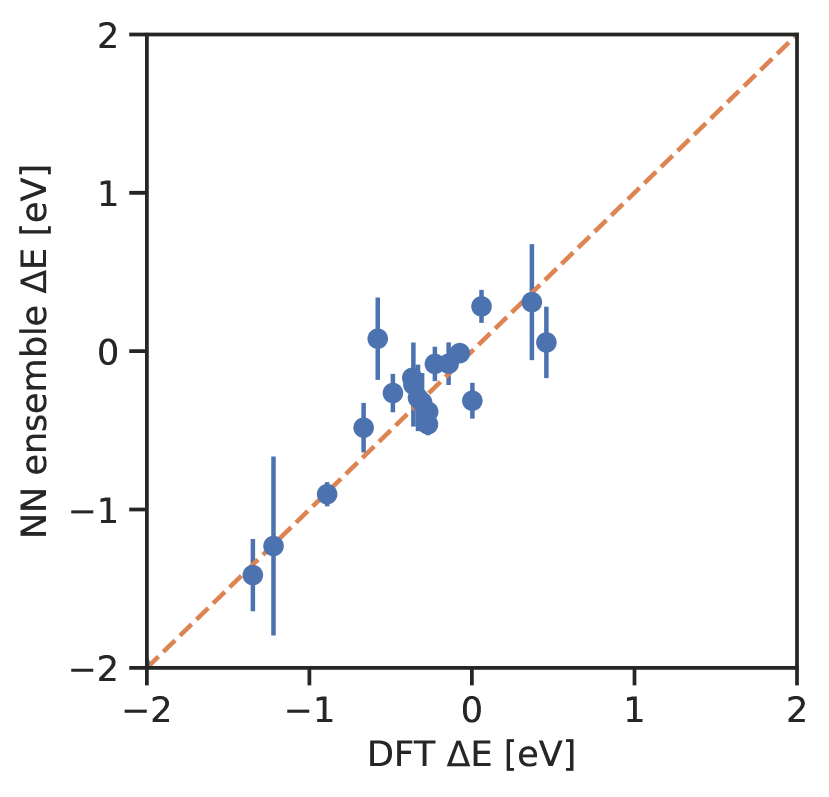
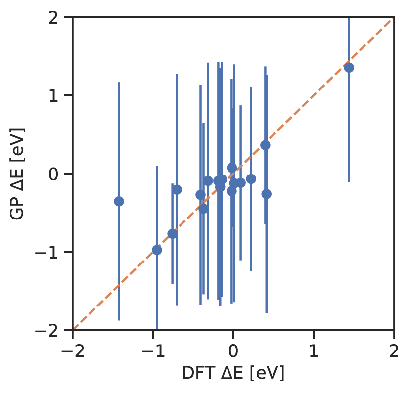
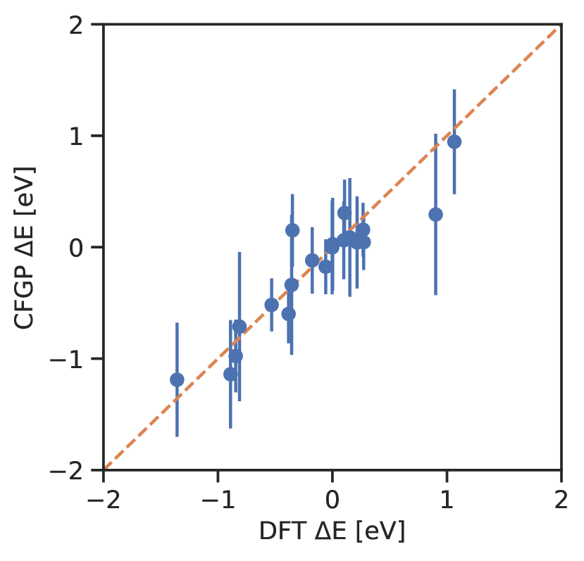
The shape of a calibration curve could also yield other insights. If a model’s UQ s were too low/confident, then the normalized residuals would be too large and they would fall outside their distributions too frequently. This would result in a lower observed cumulative distributions compared to the expected cumulative distributions, which would correspond to a calibration curve that falls below the ideal diagonal. Therefore, overconfident models yield calibration curves that fall under the ideal diagonal, and underconfident models yield calibration curves that fall over the ideal diagonal. Figure 4 illustrates this point by plotting calibration curves of various models alongside their parity plots that contain error bars corresponding to $\pm$2 standard deviations. Note that when we say a calibration curve “falls under the diagonal”, we allude to curves whose right-hand-side fall under the diagonal.

(a) calibration of NN ensemble

(b) calibration of GP

(c) calibration of CFGP

(d) parity of NN ensemble

(e) parity of GP

(f) parity of CFGP

Figure 4: Calibration curves and parity plots of an overconfident NN ensemble, an underconfident GP, and better-calibrated CFGP. The vertical uncertainty bands in the parity plots indicate $\pm$2 standard deviations in the uncertainty predictions of each model. For clarity, we sampled only 20 points of the 8,289 test points to put in the parity plots. It follows that relatively overconfident models would have more points with uncertainty bands that do not cross the diagonal parity line; relatively underconfident models would have more points that cross the diagonal parity line; and a well-calibrated model would have ca. 19 out of 20 points cross the parity line.

3.2 Summary results

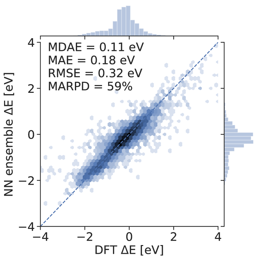
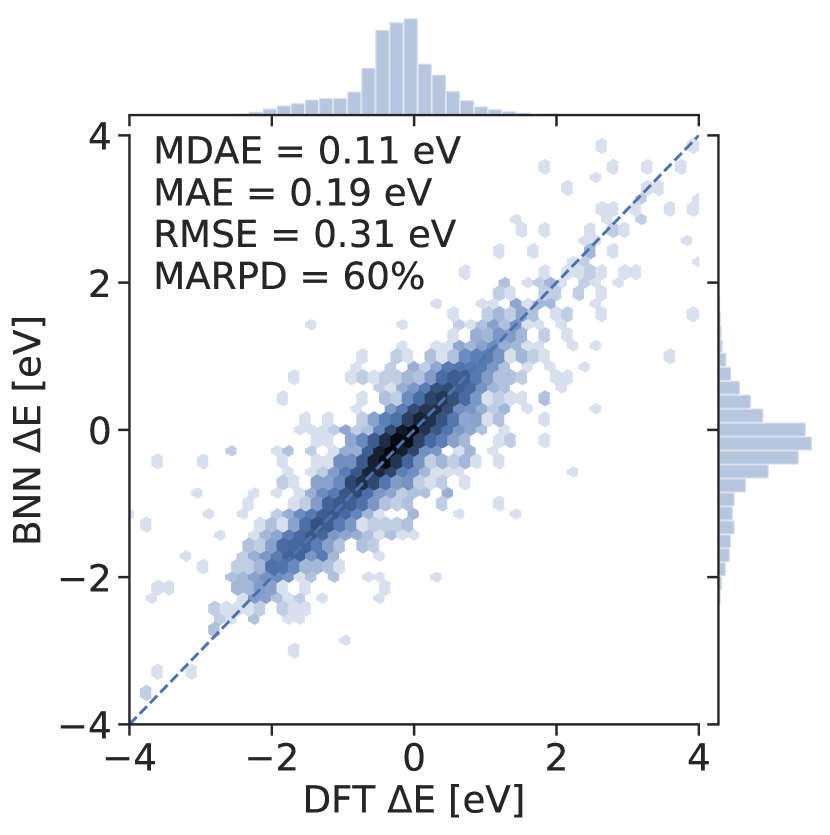
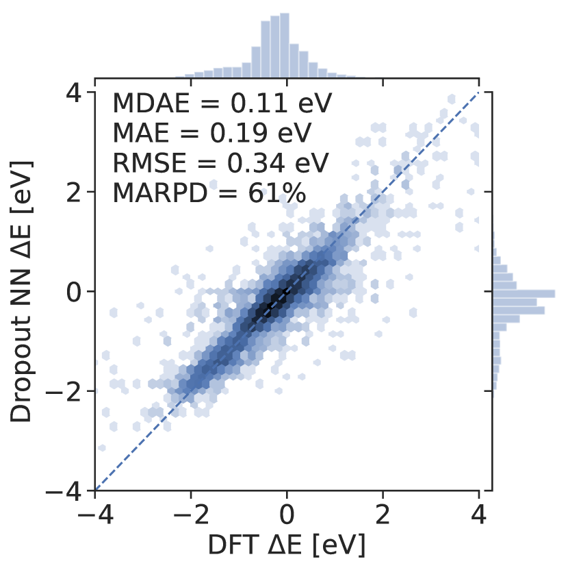
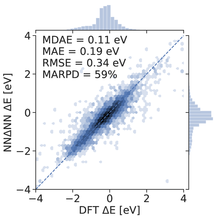
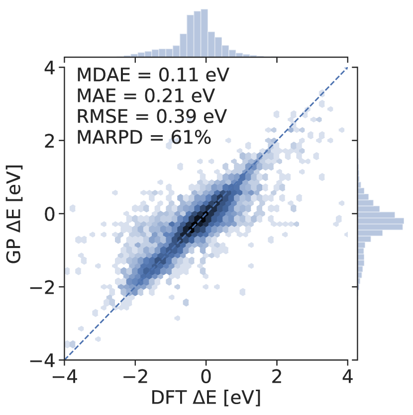
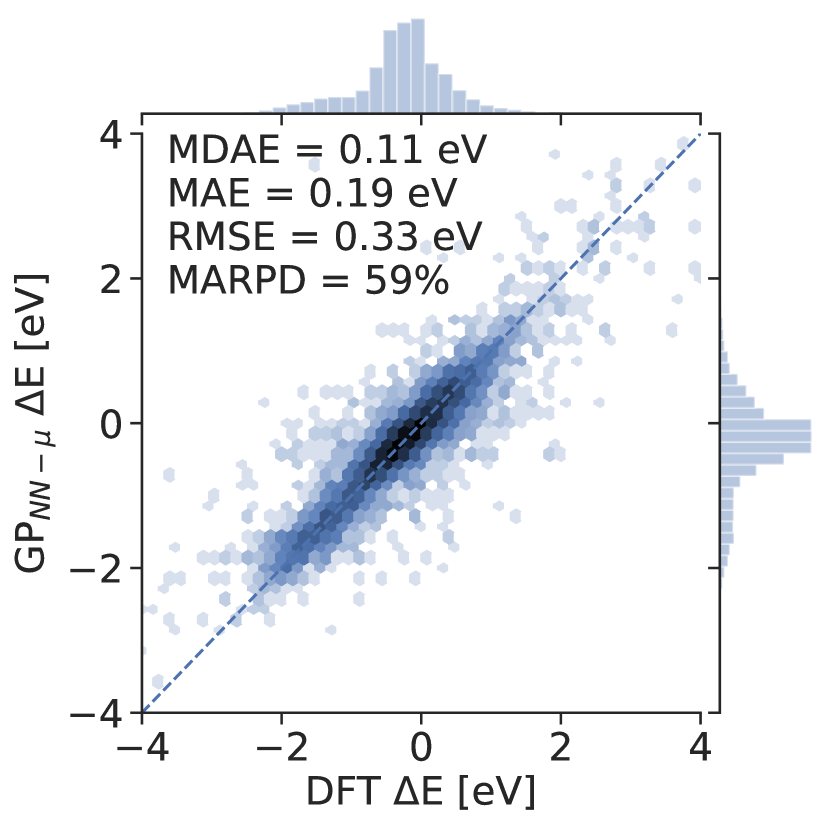
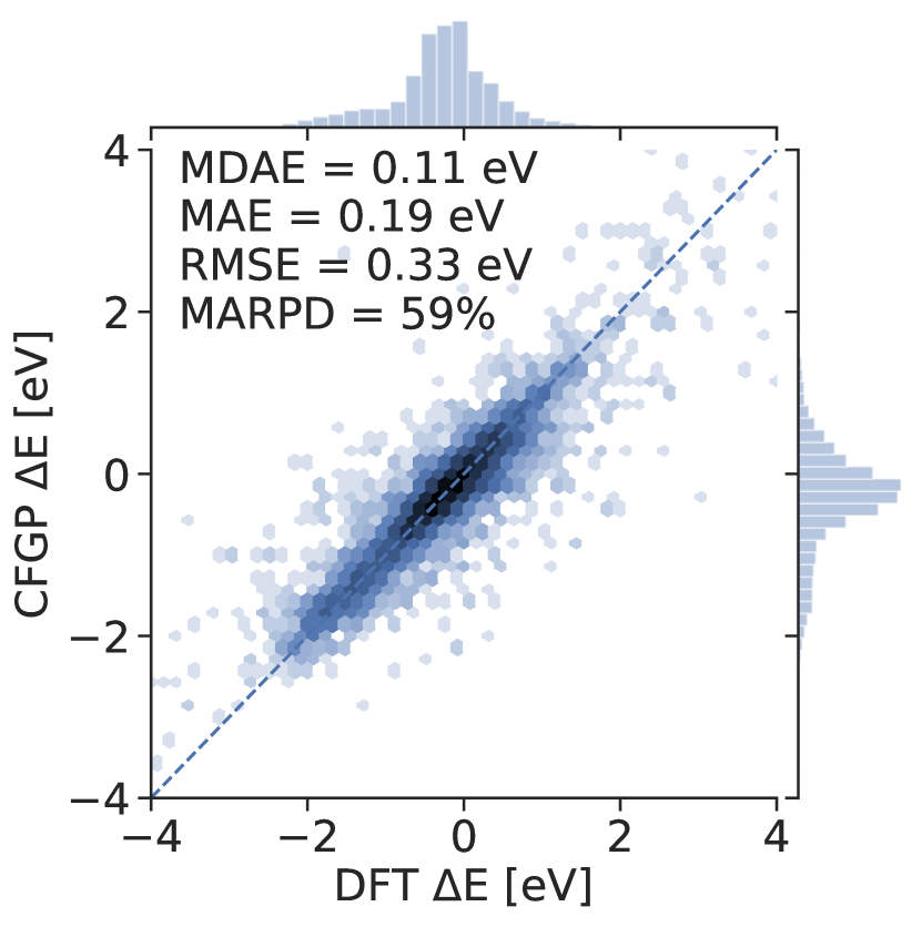
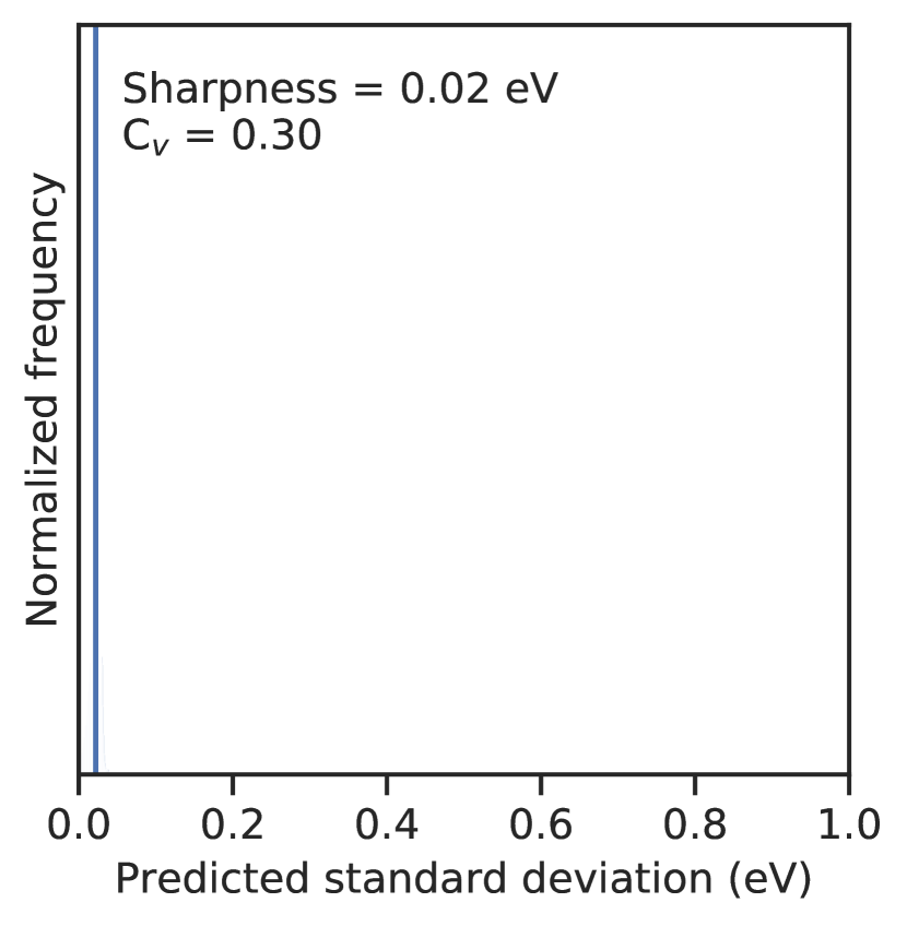
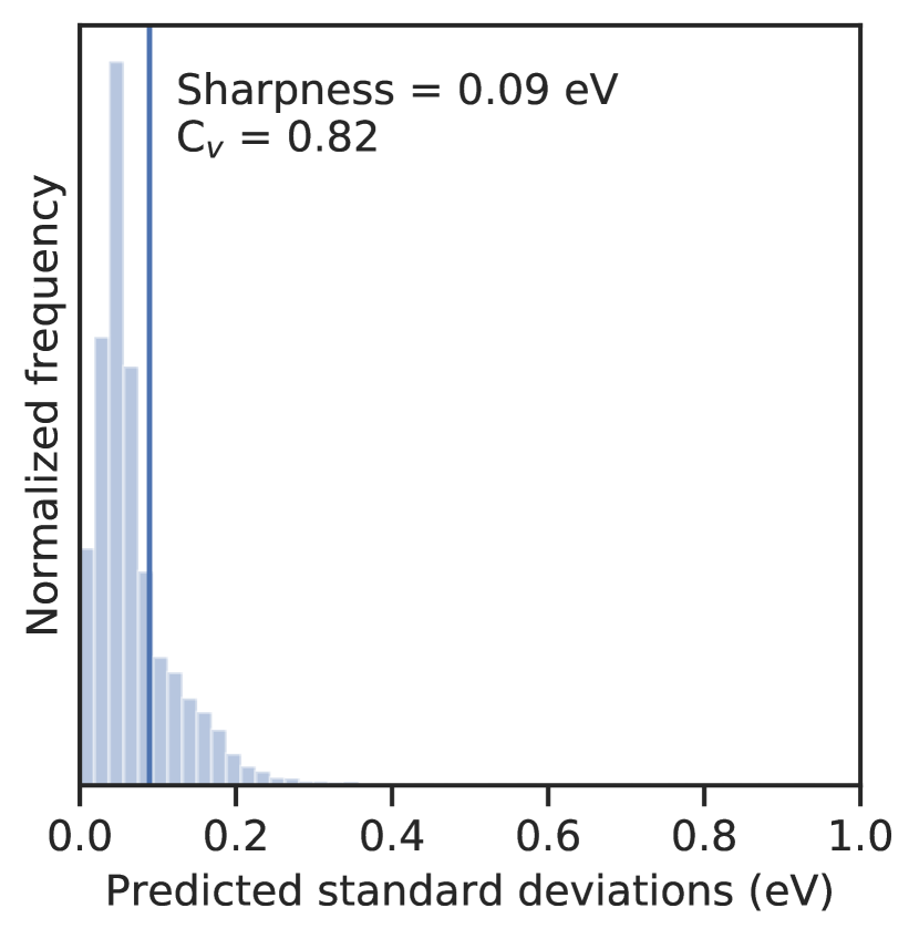
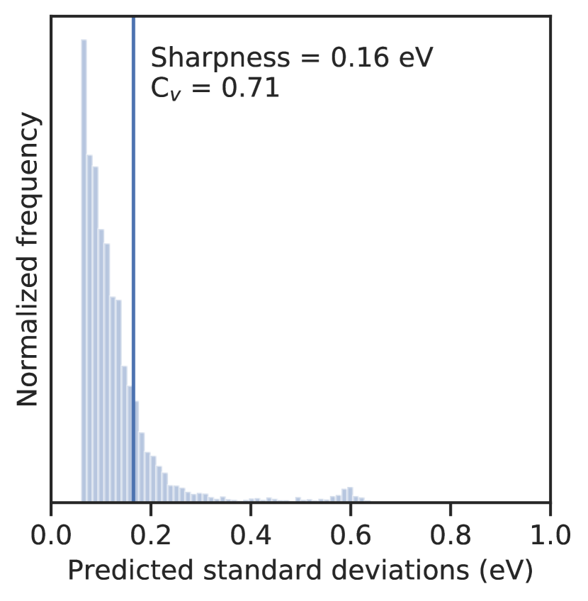
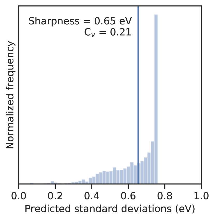
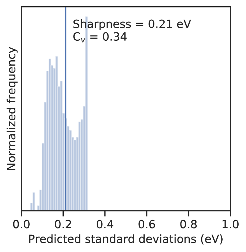
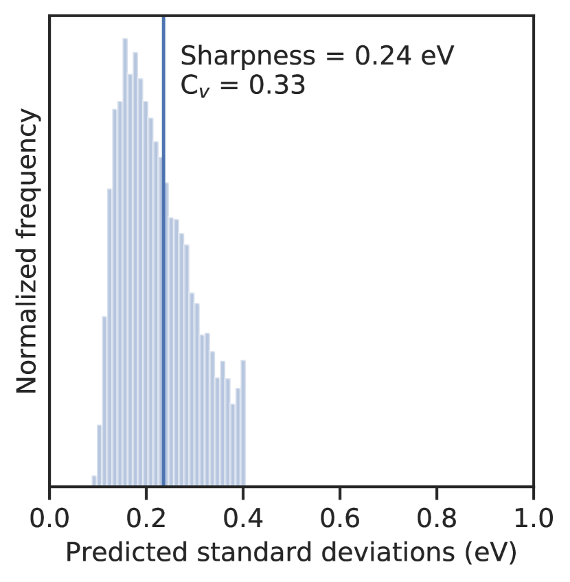
Figure 5 contains parity plots for all UQ methods studied here; Figure 6 contains all calibration curves; and Figure 7 contains all distribution plots of the ML-predicted UQ s. These figures illustrate the accuracy, calibration, and sharpness of the different UQ methods, respectively. Table 1 lists their performance metrics.

(a) NN ensemble

(b) BNN

(c) Dropout NN

(d) NN$\Delta$NN

(e) GP

(f) GP_NN-μ

(g) CFGP

Figure 5: Parity plots for all UQ methods used in this study. Shading plots were used in lieu of scatter plots because the large number of test points (8,289) obfuscated patterns. Darker shading indicates a higher density of points. Logarithmically scaled shading was used to accentuate outliers. The dashed, diagonal lines indicate parity.

(a) NN ensemble

(b) BNN

(c) Dropout NN

(d) NN$\Delta$NN

(e) GP

(f) GP_NN-μ

(g) CFGP

Figure 6: Calibration curves for all UQ methods used in this study. Dashed, blue lines indicate perfect calibration while solid orange lines indicate the experimental calibration of the test set. The blue, shaded area between these lines is defined as the miscalibration area.

(a) NN ensemble

(b) BNN

(c) Dropout NN

(d) NN$\Delta$NN

(e) GP

(f) GP_NN-μ

(g) CFGP

Figure 7: Distribution plots of the ML-predicted standard deviations for each method. Sharpness values are indicated by vertical lines.

Method	MDAE	MAE	RMSE	MARPD	R2	MisCal	CalErr	Sha	Cv	NLL $\cdot$103
NN	0.11	0.19	0.34	61	0.80	N/A	N/A	N/A	N/A	N/A
NN ensemble	0.11	0.18	0.32	59	0.82	0.12	1.70	0.14	1.06	192.08
BNN	0.11	0.19	0.31	59	0.83	0.20	5.32	0.03	0.30	669.61
Dropout NN	0.11	0.19	0.34	61	0.79	0.14	2.52	0.09	0.82	7.38$\cdot$1014
NN$\Delta$NN	0.11	0.19	0.34	59	0.80	0.05	0.39	0.16	0.71	18.61
GP	0.11	0.21	0.39	61	0.73	0.14	2.35	0.65	0.21	6.41
GPNN-μ	0.11	0.19	0.33	59	0.81	0.03	0.08	0.21	0.34	6.09
CFGP	0.11	0.19	0.33	59	0.80	0.03	0.13	0.24	0.33	2.80

Table 1: Performance metrics for all methods used in this study, which include: Median Absolute Error (MDAE), Mean Absolute Error (MAE), Root Mean Squared Error (RMSE), Mean Absolute Relative Percent Difference (MARPD), R² correlation coefficient (R²), miscalibration area (MisCal), calibration error (CalErr), sharpness (Sha), coefficient of variation (C_v), and negative log-likelihood (NLL). The units of MDAE, MAE, RMSE, and sharpness are all in eV. The units of MARPD are in %. The miscalibration area, calibration error, C_v, and NLL are unitless.

Regarding accuracy: All methods’ MDAE results are virtually identical, and their MAE results are within 10% of each other. This suggests that all methods have comparable predictive accuracies for inliers. The plain GP has a higher RMSE value than the rest of the methods, indicating that it has the worst predictive accuracy for outliers. Correlations between residuals and uncertainty estimates are discussed in the Supplementary Information section briefly.

Regarding calibration: The NN ensemble, BNN, and Dropout NN are overconfident; the GP is underconfident; and the NN$\Delta$NN, GP_NN-μ, and CFGP models are relatively calibrated. The three more calibrated methods all share a characteristic that the other methods do not: They all start with a NN that is dedicated for prediction alone, and then they end with some other in-series method to estimate uncertainty. Interestingly, this in-series method of learning predictions and then learning uncertainties is similar in spirit to how gradient boosted models “learn in stages” using an ensemble of models.

Regarding sharpness: The NN ensemble, BNN, and Dropout NN models yield the most sharp uncertainties, although they do so at the cost of calibration. Among the three more calibrated models, the NN$\Delta$NN yields the lowest sharpness of 0.16 eV while the GP_NN-μ and CFGP yield sharpnesses of 0.21 and 0.24 eV, respectively. Note how GP-based UQ methods tend to yield less sharp uncertainties than methods based purely on NN s. This suggests that GP s may yield more conservative UQ s.

Regarding NLL: The CFGP method yields the best (i.e., lowest) NLL value of ca. 2,800 while both the GP and GP_NN-μ models yield relatively moderate NLL values of ca. 6,000. Note how the under-confident GP model has a worse miscalibration area, calibration error, and sharpness than the NN$\Delta$NN but a better NLL value. Simultaneously, the three most over-confident and sharp models (NN ensemble, BNN, and Dropout NN) yield the worst NLL results. This shows that better NLL values correlate with relatively conservative estimates of UQ, but not with relatively liberal estimates. In other words: If we use NLL as our main performance metric, then we will favor under-confident UQ estimates in lieu of over-confident estimates.

Given the performance metrics for accuracy, calibration, sharpness, and NLL, we expect the CFGP or GP_NN-μ methods to yield the best performing UQ models for our dataset. When choosing UQ methods for different applications, other factors should be considered. For example: Although the GP_NN-μ method performed relatively well, it relied on hand-crafted features. If future researchers wish to use the GP_NN-μ method to predict other properties from atomic structures, they may have to define their own set of features. This process of feature engineering is non-trivial and varies from application to application. In some cases, it may be easier to use a UQ method that does not require any additional features beyond the NN input, such as NN$\Delta$NN or CFGP. This is why declare CFGP as the method of choice for our study here; it has a relatively competitive accuracy, calibration, and sharpness while requiring less information than GP_NN-μ.

Another factor to consider is the overhead cost of implementation. For example: The NN ensemble method is arguably the simplest NN-based UQ method used here and may be the easiest method to implement. Conversely, NN ensembles also have a higher computational training cost than some of the other methods used here, such as NN$\Delta$NN or CFGP. This high training cost is exacerbated if the ensemble is meant to be used in an active framework where the model needs to be trained continuously. As another example: The BNN method yielded perhaps the worst results of all the methods studied here. It could be argued that further optimization of the BNN could have resulted in higher performance. But creation and training of BNN s is still an active area of research with less literature and support than GP s or non-Bayesian NN s. This lack of support led to us spending nearly twice as long creating a BNN compared to the other methods. It follows that further optimization of the BNN would be non-trivial and may not be worth the overhead investment.

4 Conclusions

We examined a procedure for comparing different methods for uncertainty quantification (UQ). This procedure considers the accuracy of each method, the honesty of their uncertainty estimates (i.e., their calibration), and the size of their uncertainty estimates (i.e., their sharpness). To assess accuracy, we outlined a common set of error metrics such as MAE or RMSE, among others. To assess calibration, we showed how to create, interpret, and quantify calibration curves. To assess sharpness, we showed how to calculate and plot sharpness. To assess all three aspects simultaneously, we suggest using the negative log-likelihood (NLL) as a performance metric. The ensemble of all these metrics and figures can be used to judge the relative performance of various UQ methods in a holistic fashion.

As a case study, we tested six different methods for predicting Density Functional Theory (DFT) calculated adsorption energies with UQ. The best performing method was a Convolution-Fed Gaussian Process (CFGP), which used a pre-trained convolutional output from a NN as features for a subsequent GP that made probabilistic predictions. Our studies also showed that the GP-based methods we tested tended to yield higher and more conservative uncertainty estimates than the methods that used only NN s and NN derivatives. We also found that in-series methods tended to yield more calibrated models—i.e., methods that use one model to make value predictions and then a subsequent model to make uncertainty estimates were more calibrated than models that attempted to make value and uncertainty predictions simultaneously. These results are limited to our dataset. Results may vary for studies with different applications, different models, or different hyperparameters. But the underpinning procedure we used to compare these models is still broadly applicable.

Note that it would be possible to recalibrate¹⁷ each of the models in this study to improve their uncertainty estimates. We purposefully omitted recalibration in this study to (1) simplify the illustration of the UQ assessment procedure; (2) assess the innate performance of each of these UQ methods without confounding with recalibration methods; and (3) reduce overhead investment. Future work should consider recalibration if the feasible UQ methods provide insufficiently calibrated uncertainty predictions

Future work may also consider inductively biased UQ s. For example: If we used the Bayesian Error Estimation Functional with van der Waals correlation (BEEF-vdW),³⁸ then our DFT calculated adsorption energies would have been distributions rather than than single point estimates. Such distributions could be propagated to certain UQ surrogate models, e.g., as a variable-variance kernel in a GP-type method. As another example of inductively biased UQ s: A model may be able to make low-uncertainty predictions on a DFT-optimized structure and then also make high-uncertainty predictions on a similar but DFT-unoptimized structure. UQ s do not need to be derived strictly from data. They may also be derived from previous knowledge.

Author information

Corresponding author email: zulissi@andrew.cmu.edu. The authors declare no competing financial interest.

Code availability

Visit https://github.com/ulissigroup/uncertainty_benchmarking for the code used to create the results discussed in this paper. The code dependencies are listed inside the repository.

Data availability

The data that support the findings of this study are available from the corresponding author upon reasonable request.

References

- Medford et al. 2018 Medford, A. J.; Kunz, M. R.; Ewing, S. M.; Borders, T.; Fushimi, R. Extracting Knowledge from Data through Catalysis Informatics. ACS Catalysis 2018, 8, 7403–7429
- Gu et al. 2019 Gu, G. H.; Noh, J.; Kim, I.; Jung, Y. Machine learning for renewable energy materials. Journal of Materials Chemistry A 2019, 7, 17096–17117
- Schleder et al. 2019 Schleder, G. R.; Padilha, A. C. M.; Acosta, C. M.; Costa, M.; Fazzio, A. From DFT to Machine Learning: recent approaches to Materials Science – a review. Journal of Physics: Materials 2019, 2, 1–46
- Alberi et al. 2019 Alberi, K. et al. The 2019 materials by design roadmap. J. Phys. D: Appl. Phys 2019, 52, 1–48
- Settles 2012 Settles, B. In Synthesis Lectures on Artificial Intelligence and Machine Learning; Brachman, R. J., Cohen, W. W., Dietterich, T. G., Eds.; Morgan & Claypool, 2012; p 100
- Chu et al. 2011 Chu, W.; Zinkevich, M.; Li, L.; Thomas, A.; Tseng, B. Unbiased online active learning in data streams. Proceedings of the ACM SIGKDD International Conference on Knowledge Discovery and Data Mining 2011, 195–203
- Frazier 2018 Frazier, P. I. A Tutorial on Bayesian Optimization. 2018
- Garnett et al. 2012 Garnett, R.; Krishnamurthy, Y.; Xiong, X.; Schneider, J.; Mann, R. Bayesian optimal active search and surveying. Proceedings of the 29th International Conference on Machine Learning, ICML 2012 2012, 2, 1239–1246
- Kandasamy et al. 2018 Kandasamy, K.; Neiswanger, W.; Zhang, R.; Krishnamurthy, A.; Schneider, J.; Poczos, B. Myopic Bayesian Design of Experiments via Posterior Sampling and Probabilistic Programming. 2018
- Peterson 2016 Peterson, A. A. Acceleration of saddle-point searches with machine learning. Journal of Chemical Physics 2016, 145
- Torres et al. 2018 Torres, J. A. G.; Jennings, P. C.; Hansen, M. H.; Boes, J. R.; Bligaard, T. Low-Scaling Algorithm for Nudged Elastic Band Calculations Using a Surrogate Machine Learning Model. 2018, 156001, 1–6
- Jinnouchi et al. 2019 Jinnouchi, R.; Lahnsteiner, J.; Karsai, F.; Kresse, G.; Bokdam, M. Phase Transitions of Hybrid Perovskites Simulated by Machine-Learning Force Fields Trained on the Fly with Bayesian Inference. Physical Review Letters 2019, 122, 225701
- Peterson et al. 2017 Peterson, A. A.; Christensen, R.; Khorshidi, A. Addressing uncertainty in atomistic machine learning. Phys. Chem. Chem. Phys. Phys. Chem. Chem. Phys 2017, 19, 10978–10985
- Musil et al. 2019 Musil, F.; Willatt, M. J.; Langovoy, M. A.; Ceriotti, M. Fast and Accurate Uncertainty Estimation in Chemical Machine Learning. Journal of Chemical Theory and Computation 2019, 15, 906–915
- Janet et al. 2019 Janet, J. P.; Duan, C.; Yang, T.; Nandy, A.; Kulik, H. J. A quantitative uncertainty metric controls error in neural network-driven chemical discovery. Chemical Science 2019, 10, 7913–7922
- Scalia et al. 2019 Scalia, G.; Grambow, C. A.; Pernici, B.; Li, Y.-P.; Green, W. H. Evaluating Scalable Uncertainty Estimation Methods for DNN-Based Molecular Property Prediction. 2019; \urlhttp://arxiv.org/abs/1910.03127
- Kuleshov et al. 2018 Kuleshov, V.; Fenner, N.; Ermon, S. Accurate Uncertainties for Deep Learning Using Calibrated Regression. 35th International Conference on Machine Learning. Stockholm, Sweden, 2018
- Levi et al. 2020 Levi, D.; Gispan, L.; Giladi, N.; Fetaya, E. Evaluating and Calibrating Uncertainty Prediction in Regression Tasks. 2020; \urlhttp://arxiv.org/abs/1905.11659
- Tran and Ulissi 2018 Tran, K.; Ulissi, Z. W. Active learning across intermetallics to guide discovery of electrocatalysts for CO2 reduction and H2 evolution. Nature Catalysis 2018, 1, 696–703
- Tran et al. 2018 Tran, K.; Aini, P.; Back, S.; Ulissi, Z. W. Dynamic Workflows for Routine Materials Discovery in Surface Science. Journal of Chemical Information and Modeling 2018, 58, 2392–2400
- Kresse and Hafner 1993 Kresse, G.; Hafner, J. Ab initio molecular dynamics for liquid metals. Physical Review B 1993, 47, 558–561
- Kresse and Hafner 1994 Kresse, G.; Hafner, J. Ab initio molecular-dynamics simulation of the liquid-metal–amorphous-semiconductor transition in germanium. Physical Review B 1994, 49, 14251–14269
- Kresse and Furthmüller 1996 Kresse, G.; Furthmüller, J. Efficiency of ab-initio total energy calculations for metals and semiconductors using a plane-wave basis set. Computational Materials Science 1996, 6, 15–50
- Kresse and Furthmüller 1996 Kresse, G.; Furthmüller, J. Efficient iterative schemes for ab initio total-energy calculations using a plane-wave basis set. Physical Review B 1996, 54, 11169–11186
- Hjorth Larsen et al. 2017 Hjorth Larsen, A. et al. The atomic simulation environment—a Python library for working with atoms. Journal of Physics: Condensed Matter 2017, 29, 273002
- Hammer et al. 1999 Hammer, B.; Hansen, L. B.; Nørskov, J. Improved adsorption energetics within density-functional theory using revised Perdew-Burke-Ernzerhof functionals. Physical Review B 1999, 59, 7413–7421
- Thompson 2012 Thompson, S. K. In Sampling, 3rd ed.; Shewhart, W. A., Wilks, S. S., Eds.; John Wiley and Sons Inc., 2012; Chapter 11, pp 139–156
- Meredig et al. 2018 Meredig, B.; Antono, E.; Church, C.; Hutchinson, M.; Ling, J.; Paradiso, S.; Blaiszik, B.; Foster, I.; Gibbons, B.; Hattrick-Simpers, J.; Mehta, A.; Ward, L. Can machine learning identify the next high-temperature superconductor? Examining extrapolation performance for materials discovery. Molecular Systems Design and Engineering 2018, 3, 819–825
- Hyndman and Athanasopoulos 2014 Hyndman, R. J.; Athanasopoulos, G. Forecasting: Principles and practice, 1st ed.; otexts.com, 2014
- Xie and Grossman 2018 Xie, T.; Grossman, J. C. Crystal Graph Convolutional Neural Networks for an Accurate and Interpretable Prediction of Material Properties. Physical Review Letters 2018, 120, 145301
- Back et al. 2019 Back, S.; Yoon, J.; Tian, N.; Zhong, W.; Tran, K.; Ulissi, Z. W. Convolutional Neural Network of Atomic Surface Structures To Predict Binding Energies for High-Throughput Screening of Catalysts. The Journal of Physical Chemistry Letters 2019, 10, 4401–4408
- Bingham et al. 2018 Bingham, E.; Chen, J. P.; Jankowiak, M.; Obermeyer, F.; Pradhan, N.; Karaletsos, T.; Singh, R.; Szerlip, P.; Horsfall, P.; Goodman, N. D. Pyro: Deep Universal Probabilistic Programming. 2018, 0–5
- Gal and Ghahramani 2016 Gal, Y.; Ghahramani, Z. Dropout as a Bayesian Approximation : Representing Model Uncertainty in Deep Learning. 33rd International Conference on Machine Learning. New York, NY, USA, 2016
- Gardner et al. 2018 Gardner, J. R.; Pleiss, G.; Bindel, D.; Weinberger, K. Q.; Wilson, A. G. GPyTorch: Blackbox Matrix-Matrix Gaussian Process Inference with GPU Acceleration. 32nd Conference on Neural Information Processing Systems (NeurIPS). 2018
- Gneiting and Raftery 2007 Gneiting, T.; Raftery, A. E. Strictly proper scoring rules, prediction, and estimation. Journal of the American Statistical Association 2007, 102, 359–378
- Dawid and Musio 2014 Dawid, A. P.; Musio, M. Theory and applications of proper scoring rules. Metron 2014, 72, 169–183
- Lakshminarayanan et al. 2017 Lakshminarayanan, B.; Pritzel, A.; Blundell, C. Simple and Scalable Predictive Uncertainty Estimation using Deep Ensembles. 31st Conference on Neural Information Processing Systems (NIPS). 2017
- Wellendorff et al. 2012 Wellendorff, J.; Lundgaard, K. T.; Møgelhøj, A.; Petzold, V.; Landis, D. D.; Nørskov, J. K.; Bligaard, T.; Jacobsen, K. W. Density functionals for surface science: Exchange-correlation model development with Bayesian error estimation. Physical Review B - Condensed Matter and Materials Physics 2012, 85, 32–34