Non-minimal (self-)running inflation:
metric vs. Palatini formulation

Abstract

We consider a model of quartic inflation where the inflaton is coupled non-minimally to gravity and the self-induced radiative corrections to its effective potential are dominant. We perform a comparative analysis considering two different formulations of gravity, metric or Palatini, and two different choices for the renormalization scale, widely known as prescription I and II. Moreover we comment on the eventual compatibility of the results with the final data release of the Planck mission.

1 Introduction

According to the theory of cosmic inflation Starobinsky:1980te ; Guth:1980zm ; Linde:1981mu ; Albrecht:1982wi , our Universe underwent a period of exponential expansion during the initial moments of its life. Inflation has the merit of providing at the same time a solution to issues like the flatness and horizon problems of the Universe and a way to generate primordial inhomogeneities, whose power spectrum is currently being tested in several experiments Ade:2015tva ; Ade:2015xua ; Ade:2015lrj ; Array:2015xqh ; Planck2018:inflation . In particular, the final data release of the Planck mission Planck2018:inflation casts strong constraints on the tensor-to-scalar ratio $r$, an observable related to the amplitude of primordial gravitational waves and to the scale of inflation. As a consequence, the predictions of the simple monomial inflation models are ruled out at $2\sigma$ level, leaving non-minimally coupled to gravity models as some of the most favorite ones. In this article we are going to study models of inflation with a non-minimal coupling to gravity of the type $\xi\phi^{2}R$, where $\phi$ is the inflaton field, $R$ the Ricci scalar and $\xi$ a coupling constant. Similar models have been studied in a large number of works over the past decades (in e.g.Futamase:1987ua ; Salopek:1988qh ; Fakir:1990eg ; Amendola:1990nn ; Kaiser:1994vs ; Bezrukov:2007ep ; Park:2008hz ; Linde:2011nh ; Kaiser:2013sna ; Kallosh:2013maa ; Kallosh:2013daa ; Kallosh:2013tua ; Galante:2014ifa ; Jarv:2016sow ; Chiba:2014sva ; Boubekeur:2015xza ; Pieroni:2015cma ; Salvio:2017xul ; Bostan:2018evz ; Almeida:2018pir ; Cheng:2018axr ; Tang:2018mhn ; SravanKumar:2018tgk ; Kubo:2018kho ; Canko:2019mud ; Okada:2019opp ; Karam:2017rpw ; Karam:2018mft ). These models are particular interesting, since non-minimal couplings should be interpreted as a generic ingredient of consistent model building, arising from quantum corrections in a curved space-time Birrell:1982ix . In particular, this is the case for the scenario where the Standard Model Higgs scalar is the inflaton field Bezrukov:2007ep . Comparisons of non-minimally coupled models of chaotic inflation were performed in e.g. Linde:2011nh ; Kaiser:2013sna ; Kallosh:2013maa ; Kallosh:2013daa ; Kallosh:2013tua ; Galante:2014ifa ; Jarv:2016sow . In Refs. Kaiser:2013sna ; Kallosh:2013tua , it was shown that for large values of the non-minimal coupling, all models, independently of the original scalar potential, asymptote to a universal attractor: the Starobinsky model Starobinsky:1980te . However, the presence of non-minimal couplings to gravity requires a discussion about the gravitational degrees of freedom. In the usual metric formulation of gravity the independent variables are the metric and its first derivatives, while in the Palatini formulation the independent variables are the metric and the connection. Using the Einstein-Hilbert Lagrangian, the two formalisms predict the same equations of motion and therefore describe equivalent physical theories. However, with non-minimal couplings between gravity and matter, such equivalence is lost and the two formulations describe different gravity theories Bauer:2008zj and lead to different phenomenological results, as recently investigated in e.g. Bauer:2010jg ; Tamanini:2010uq ; Tenkanen:2017jih ; Jarv:2017azx ; Rasanen:2018ihz ; Carrilho:2018ffi ; Almeida:2018oid ; Takahashi:2018brt ; Antoniadis:2018yfq ; Tenkanen:2019jiq ; Tenkanen:2019xzn ; Tenkanen:2019wsd ; Bostan:2019wsd ; Gialamas:2019nly ; Rasanen:2017ivk ; Kannike:2018zwn ; Enckell:2018kkc ; Racioppi:2017spw ; Racioppi:2018zoy ; Antoniadis:2018ywb ; Bostan:2019uvv ; Markkanen:2017tun ; Enckell:2018hmo ; Kozak:2018vlp . In particular, the attractor behaviour of the so-called $\xi$ attractor models Kallosh:2013tua is lost in the Palatini formulation Jarv:2017azx . It is important to remark that in Kallosh:2013tua ; Jarv:2017azx the role of quantum corrections is implicitily assumed to be subdominant. On the other side, it has been demonstrated that radiative corrections to inflationary potentials may play a relevant role Kannike:2014mia ; Marzola:2015xbh ; Marzola:2016xgb ; Dimopoulos:2017xox , dynamically generating the Planck scale Kannike:2015apa ; Kannike:2015kda , predicting super-heavy dark matter Farzinnia:2015fka ; Kannike:2016jfs and leading to linear inflation predictions when a non-minimal coupling to gravity is added Kannike:2015kda ; Rinaldi:2015yoa ; Barrie:2016rnv ; Artymowski:2016dlz ; Racioppi:2017spw ; Racioppi:2018zoy .

At the present date, all the comparative studies between the metric and Palatini formulations either consider only a classical tree-level analysis Bauer:2008zj ; Bauer:2010jg ; Tamanini:2010uq ; Tenkanen:2017jih ; Jarv:2017azx ; Rasanen:2018ihz ; Carrilho:2018ffi ; Almeida:2018oid ; Takahashi:2018brt ; Antoniadis:2018yfq ; Tenkanen:2019jiq ; Tenkanen:2019xzn ; Tenkanen:2019wsd ; Bostan:2019wsd ; Gialamas:2019nly or assume that the leading contribution to radiative corrections is coming from some other additional particle (inside the Standard Model Rasanen:2017ivk ; Kannike:2018zwn ; Enckell:2018kkc or beyond it Racioppi:2017spw ; Racioppi:2018zoy ; Antoniadis:2018ywb ; Bostan:2019uvv ) rather than the inflaton itself. While there have been several works about self-induced radiative corrections for a non-minimal inflaton in the metric case (e.g. Buchbinder:1992rb ; Elizalde:1993ew ; Inagaki:2015fva ; George:2013iia ), such a topic is completely unexplored in the Palatini one. Therefore, the aim of this work is to fill the gap in the literature and present for the first time a comparative analysis of the possible gravity formulation (metric or Palatini) in the context of non-minimal inflation when self-corrections are the dominant loop contribution.

The article is organized as follows. In section 2 we set the notation reintroducing the main concepts about running coupling constants and the effective potential. In section 3 we discuss the gravitational sector and the main differences between the metric and the Palatini formulation of a gravity theory. In section 4 we present the comparative study of the inflationary predictions. We conclude in section 5.

2 Model building and effective potential

Consider the following action for a scalar-tensor theory in the Jordan frame

$$S=\!\!\int\!\!d^{4}x\sqrt{-g}\left(-\frac{M_{P}^{2}}{2}f(\phi)R(\Gamma)+\frac{(\partial\phi)^{2}}{2}-V_{\rm eff}(\phi)\right),$$ (1)

where $M_{P}$ is the reduced Planck mass, $R$ is the Ricci scalar constructed from a connection $\Gamma$ and $V_{\rm eff}(\phi)$ is the effective potential of the inflaton scalar. In the following we will focus on one particular type of $f$ function:

$$f(\phi)=1+\xi\frac{\phi^{2}}{M_{P}^{2}}\,,$$ (2)

which is the usual Higgs-inflation Bezrukov:2007ep non-minimal coupling where we relaxed the condition that the inflaton is the Higgs boson and allowed the possibility that inflation is driven by another scalar beyond the Standard Model particle content. The tree-level inflaton potential is

$$V(\phi)=\frac{1}{4}\lambda\phi^{4}\,,$$ (3)

however our focus is on the 1-loop improved effective inflaton potential. Assuming that only self-corrections are relevant during inflation, the improved potential is

$$V_{\rm eff}(\phi,\mu)=\frac{1}{4}\lambda_{\rm eff}(\phi,\mu)\phi^{4}$$ (4)

where the effective quartic coupling is

$$\lambda_{\rm eff}(\phi,\mu)=\lambda(\mu)+\frac{9\lambda(\mu)^{2}}{16\pi^{2}}\ln\left[\frac{3\lambda(\mu)\phi^{2}}{\mu^{2}}\right]\,.$$ (5)

The second part of eq. (5) is the contribution coming from the Coleman-Weinberg (CW) 1-loop correction Coleman:1973jx to the effective potential, while the first one comes from the renormalization group equation (RGE) PhysRevD.2.1541 ; Symanzik1970 of the quartic coupling, whose solution is

$$\lambda(\mu)=\frac{\lambda_{0}}{1-\frac{9\lambda_{0}\ln\left(\frac{\mu^{2}}{\mu_{0}^{2}}\right)}{16\pi^{2}}}\,,$$ (6)

where $\lambda_{0}=\lambda(\mu_{0})$ is the boundary condition for the RGE. For convenience we choose $\mu_{0}={M_{\rm P}}$ and keep $\lambda_{0}$ as a free parameter. It is important to keep in mind that the solution (5) is correct at the order $O(\lambda^{2}(\mu))$, therefore any $\mu$-dependence at higher order can be thrown away and the effective coupling can be safely truncated as

$$\lambda_{\rm eff}(\phi,\mu)=\lambda(\mu)+\frac{9\lambda(\mu)^{2}}{16\pi^{2}}\ln\left(\frac{3\lambda_{0}\phi^{2}}{\mu^{2}}\right)\,.$$ (7)

The purpose of the RGE improved effective potential is to obtain a potential that, at a given perturbative order, is independent on the choice of $\mu$ (e.g. Neubert:2019mrz and references therein). Therefore, in the regime of validity of the RGE, i.e. until $\lambda(\mu)$ is small enough, any choice of $\mu$ is equivalent and should not carry any physical meaning Neubert:2019mrz . Any effect coming from the choice of $\mu$ should be due to the loss of validity of the 1-loop expansion in eq. (7) and the need for a result at least at 2-loops. However there are two choices which are quite popular and eventually convenient, which are Bezrukov:2013fka ; Allison:2013uaa ; Hamada:2016onh ; Bostan:2019fvk

$$\mu_{\rm I}^{2}=\frac{3\lambda_{0}\phi^{2}}{f(\phi)}$$ (8)

also known as prescription I and

$$\mu_{\rm II}^{2}=3\lambda_{0}\phi^{2}$$ (9)

also known as prescription II. Prescription I Bezrukov:2012hx is the choice motivated by the scale-invariant quantization in the Jordan frame, while prescription II DeSimone:2008ei ; Barvinsky:2009fy ; Barvinsky:2009ii corresponds to the usual quantization in the Jordan frame and it is convenient because it cancels explicitly the CW part of (7), moving all the loop correction into the running of the quartic coupling. For convenience later on we will use the following notation: $\lambda_{\rm eff}(\phi,\mu_{\rm I,II})=\lambda_{\rm I,II}(\phi)$.

It is also useful to notice that in case of very small $\lambda_{0}$, the dependence on $\mu$ explicitly cancels away. Performing a Taylor expansion of eq. (7) till the 2nd order in $\lambda_{0}$ we get the following approximated effective coupling

$$\lambda_{\rm app}(\phi) \simeq \lambda_{0}+\frac{9\lambda_{0}^{2}}{16\pi^{2}}\ln\left(\frac{\mu^{2}}{{M_{\rm P}}^{2}}\right)+\frac{9\lambda_{0}^{2}}{16\pi^{2}}\ln\left(\frac{3\lambda_{0}\phi^{2}}{\mu^{2}}\right)=$$ (10)

$$= \lambda_{0}+\frac{9\lambda_{0}^{2}}{16\pi^{2}}\ln\left(\frac{3\lambda_{0}\phi^{2}}{{M_{\rm P}}^{2}}\right)\,,$$

and the dependence on $\mu$ is completely removed. We notice that such expression recalls the running quartic coupling used in Racioppi:2018zoy with $\delta=\frac{9\lambda_{0}}{8\pi^{2}}$, therefore we expect that some of the results of Racioppi:2018zoy will be valid also here.

Because of perturbativity of the theory, the inflationary predictions of such a potential, in absence of a non-minimal coupling to gravity, are pretty similar to the ones of the tree-level quartic potential and already ruled out by data Planck2018:inflation . Such predictions are dramatically changed if a non-minimal coupling to gravity is added, as we do in Lagrangian (1). However, a modification of gravity calls for a discussion of what theory of gravity we are going to consider. This will be shortly discussed in the following section.

3 Non-minimal gravity

We discuss now the gravitational sector and its non-minimal coupling to the inflaton. In the metric formulation the connection is determined uniquely in function of the metric tensor, i.e. it is the Levi-Civita connection $\bar{\Gamma}=\bar{\Gamma}(g^{\mu\nu})$

$$\overline{\Gamma}^{\lambda}_{\alpha\beta}=\frac{1}{2}g^{\lambda\rho}\left(\partial_{\alpha}g_{\beta\rho}+\partial_{\beta}g_{\rho\alpha}-\partial_{\rho}g_{\alpha\beta}\right)\,.$$ (11)

On the other hand, in the Palatini formalism both $g_{\mu\nu}$ and $\Gamma$ are treated as independent variables, and the only constraint is that the connection is torsion-free, $\Gamma^{\lambda}_{\alpha\beta}=\Gamma^{\lambda}_{\beta\alpha}$. By solving the equations of motion we obtain Bauer:2008zj

$$\Gamma^{\lambda}_{\alpha\beta}=\overline{\Gamma}^{\lambda}_{\alpha\beta}+\delta^{\lambda}_{\alpha}\partial_{\beta}\omega(\phi)+\delta^{\lambda}_{\beta}\partial_{\alpha}\omega(\phi)-g_{\alpha\beta}\partial^{\lambda}\omega(\phi)\,,$$ (12)

where

$$\omega\left(\phi\right)=\ln\sqrt{f(\phi)}\,.$$ (13)

Since the connections (11) and (12) are different, the metric and Palatini formulations provide indeed two different theories of gravity. Alternatively we can understand the differences by studying the problem in the Einstein frame via the conformal transformation

$$g_{\mu\nu}^{E}=f(\phi)\ g_{\mu\nu}\,.$$ (14)

In the Einstein frame gravity looks the same in both the formulations (see also eq. (12)), however the matter sector (in our case $\phi$) behaves differently. Performing the computations Bauer:2008zj , the Einstein frame Lagrangian becomes

$$\sqrt{-g^{E}}\mathcal{L}^{E}=\sqrt{-g^{E}}\Bigg{[}-\frac{M_{P}^{2}}{2}R+\frac{(\partial\chi)^{2}}{2}-U(\chi)\Bigg{]}\,,$$ (15)

where $\chi$ is canonically normalized scalar field in the Einstein frame, and its scalar potential is given by

$$U(\chi)=\frac{V_{\text{eff}}(\phi(\chi))}{f^{2}(\phi(\chi))}\,.$$ (16)

In the metric case, $\chi$ is derived by integrating the following equation

$$\frac{\partial\chi}{\partial\phi}=\sqrt{\frac{3}{2}\left(\frac{M_{P}}{f}\frac{\partial f}{\partial\phi}\right)^{2}+\frac{1}{f}}\,,$$ (17)

where the first term comes from the transformation of the Jordan frame Ricci scalar and the second from the rescaling of the Jordan frame scalar field kinetic term. On the other hand, in the Palatini case, the field redefinition is induced only by the rescaling of the inflaton kinetic term i.e.

$$\frac{\partial\chi}{\partial\phi}=\sqrt{\frac{1}{f}}\,,$$ (18)

where there is no contribution from the Jordan frame Ricci scalar. Therefore we can see that the difference between the two formalisms in the Einstein frame relies on the different definition of $\chi$ induced by the different non-minimal kinetic term involving $\phi$.

4 Inflationary results

In this section we investigate the phenomenological implications of the non-minimal coupling in eq. (2). Since a detailed discussion of reheating is beyond the purpose of the present article, we do not need to specify the exact shape of the potential around its minimum. It is sufficient to assume that during inflation the potential is well described by eqs. (4) and (7). The corresponding Einstein frame scalar potential is given by

$$U(\chi) = \frac{\lambda_{\rm eff}(\phi,\mu)\,M_{P}^{4}\,\phi(\chi)^{4}}{4\left[M_{P}^{2}+\xi\phi(\chi)^{2}\right]^{2}}$$ (19)

$$= \frac{\lambda(\mu)\,M_{P}^{4}\,\phi(\chi)^{4}}{4\left[M_{P}^{2}+\xi\phi(\chi)^{2}\right]^{2}}\left[1+\frac{9\lambda(\mu)}{16\pi^{2}}\ln\left(\frac{3\lambda_{0}\phi(\chi)^{2}}{\mu^{2}}\right)\right],$$

where $\lambda(\mu)$ is given in (6) and the difference between the metric and the Palatini formulations is given by the different solution of eqs. (17) and (18).

Assuming slow-roll, the inflationary dynamics is described by the usual slow-roll parameters and the total number of $e$-folds during inflation. The slow-roll parameters are defined as

$$\epsilon\equiv\frac{1}{2}M_{\rm P}^{2}\left(\frac{1}{U}\frac{{\rm d}U}{{\rm d}\chi}\right)^{2}\,,\quad\eta\equiv M_{\rm P}^{2}\frac{1}{U}\frac{{\rm d}^{2}U}{{\rm d}\chi^{2}}\,,$$ (20)

and the number of $e$-folds as

$$N_{e}=\frac{1}{M_{\rm P}^{2}}\int_{\chi_{f}}^{\chi_{N}}{\rm d}\chi\,U\left(\frac{{\rm d}U}{{\rm d}\chi}\right)^{-1},$$ (21)

where the field value at the end of inflation, $\chi_{f}$, is defined via $\epsilon(\chi_{f})=1$. The field value $\chi_{N}$ at the time a given scale left the horizon is given by the corresponding $N_{e}$. To reproduce the correct amplitude for the curvature power spectrum, the potential has to satisfy Planck2018:inflation

$$\ln\left(10^{10}A_{s}\right)=3.044\pm 0.014\,,$$ (22)

where

$$A_{s}=\frac{1}{24\pi^{2}{M_{\rm P}}^{4}}\frac{U(\chi_{N})}{\epsilon(\chi_{N})}$$ (23)

and the other two relevant observables, i.e. the spectral index and the tensor-to-scalar ratio are expressed in terms of the slow-roll parameters by

$$n_{s} \simeq 1+2\eta-6\epsilon$$ (24)

$$r \simeq 16\epsilon,$$ (25)

respectively. Before performing a detailed numerical analysis, let us discuss the strong coupling limit, $\xi\to+\infty$. In this case the two formulations share a similar Einstein frame field redefinition

$$\chi\simeq\frac{M_{P}}{q}\left[\frac{8\pi^{2}}{9\lambda_{0}}+\ln\left(\frac{\sqrt{3\lambda_{0}}\phi}{M_{P}}\right)\right]$$ (26)

where we set in a convenient way the value $\chi=0$ and $q$ is either

$$q=q_{m}=\sqrt{\frac{\xi}{1+6\xi}}\,,$$ (27)

for metric gravity, or

$$q=q_{P}=\sqrt{\xi}\,,$$ (28)

for Palatini gravity. In the strong coupling limit the Einstein frame potential behaves like a running cosmological constant

$$\lim_{\xi\to\infty}U(\chi) \simeq \left[\lim_{\xi\to\infty}\lambda_{\rm eff}(\phi,\mu)\right]\frac{M_{P}^{4}}{4\xi^{2}}$$ (29)

If $\lambda_{0}$ is small ($\lambda_{0}\ll 1$), we can replace $\lambda_{\rm eff}$ with $\lambda_{\rm app}$ and get

$$\lim_{\xi\to\infty}U(\chi) \simeq \frac{\lambda_{0}\,M_{P}^{4}\,\phi(\chi)^{4}}{4\left[\xi\phi(\chi)^{2}\right]^{2}}\left[1+\frac{9\lambda_{0}}{16\pi^{2}}\ln\left(\frac{3\lambda_{0}\phi(\chi)^{2}}{{M_{\rm P}}^{2}}\right)\right]$$ (30)

$$= \frac{9\lambda_{0}^{2}}{32\pi^{2}}\frac{M_{P}^{3}}{\xi^{2}}q\,\chi\,.$$

We can see that in both gravity formulations the limit solution is linear inflation, with the only difference in the normalization factor $q$. As expected, this result is in agreement with Racioppi:2018zoy with $\delta=\frac{9\lambda_{0}}{8\pi^{2}}$. For $\lambda_{\rm eff}=\lambda_{\rm I}$ we have

$$\lim_{\xi\to\infty}\lambda_{\rm I} = \lim_{\xi\to\infty}\left[\lambda(\mu_{\rm I})+\frac{9\lambda(\mu_{\rm I})^{2}}{16\pi^{2}}\ln\left(\frac{3\lambda_{0}\phi^{2}}{\mu_{\rm I}^{2}}\right)\right]\simeq\frac{\lambda_{0}}{1-\frac{9\lambda_{0}\ln\left(\frac{3\lambda_{0}}{\xi}\right)}{16\pi^{2}}}+\frac{9\lambda_{0}^{2}\ln\left(\frac{\xi\phi^{2}}{M_{\text{P}}^{2}}\right)}{16\pi^{2}\left[1-\frac{9\lambda_{0}\ln\left(\frac{3\lambda_{0}}{\xi}\right)}{16\pi^{2}}\right]^{2}}$$ (31)

$$= \bar{\lambda}_{0}+\frac{9\bar{\lambda}_{0}^{2}}{16\pi^{2}}\ln\left(\frac{3\bar{\lambda}_{0}\phi^{2}}{\bar{\mu}_{0}^{2}}\right)$$

where

$$\bar{\lambda}_{0}=\frac{\lambda_{0}}{1-\frac{9\lambda_{0}\ln\left(\frac{3\lambda_{0}}{\xi}\right)}{16\pi^{2}}}\qquad{\rm and}\qquad\bar{\mu}_{0}=\sqrt{\frac{3\bar{\lambda}_{0}}{\xi}}M_{\text{P}}$$ (32)

It is interesting to notice that eq. (31) is the same as $\lambda_{\rm app}$ in eq. (10) with the replacements $\lambda_{0}\to\bar{\lambda}_{0}$ and $\mu_{0}\to\bar{\mu}_{0}$. Therefore we expect that inflationary results for $\lambda_{\rm eff}=\lambda_{\rm app,I}$ will be the same in the strong coupling limit, but for different values of $\lambda_{0}$ and $\xi$. And again this holds independently on the formulation of gravity. Finally, for $\lambda_{\rm eff}=\lambda_{\rm II}$ we have

$$\lim_{\xi\to\infty}\lambda_{\rm II} = \lambda(\mu_{\rm II})+\frac{9\lambda(\mu_{\rm II})^{2}}{16\pi^{2}}\ln\left(\frac{3\lambda_{0}\phi^{2}}{\mu_{\rm II}^{2}}\right)=\frac{\lambda_{0}}{1-\frac{9\lambda_{0}\ln\left(\frac{3\lambda_{0}\phi^{2}}{M_{\text{P}}^{2}}\right)}{16\pi^{2}}}$$ (33)

and therefore

$$\lim_{\xi\to\infty}U(\chi) \simeq \frac{\lambda_{0}}{1-\frac{9\lambda_{0}}{8\pi^{2}}\frac{q\,\bar{\chi}}{{M_{\rm P}}}}\frac{M_{P}^{4}}{4\xi^{2}}\,,$$ (34)

where we used eq. (26) and

$$\bar{\chi}=\chi-\frac{M_{P}}{q}\frac{8\pi^{2}}{9\lambda_{0}}\,.$$ (35)

In this case the potential does not resemble the behaviour of linear inflation, in contrast to what happens with $\lambda_{\rm eff}=\lambda_{\rm app,I}$. Moreover by using eq. (24) we get

$$n_{s}\simeq 1+\left[\frac{9\,q\,\lambda_{0}}{8\pi^{2}\left(1-\frac{9\lambda_{0}q\bar{\chi}}{8\pi^{2}M_{\text{P}}}\right)}\right]^{2}\,,$$ (36)

which means that $n_{s}\gtrsim 1$ and the strong coupling limit of $\lambda_{\rm eff}=\lambda_{\rm II}$ is ruled out.

For completeness, we perform a full inflationary analysis considering also $\xi$ values not in the strong coupling limit. We proceed in the following way. We first fix the gravity formulation (metric or Palatini) and then the effective coupling that we want to study ($\lambda_{\rm eff}=\lambda_{\rm app},\lambda_{\rm I},\lambda_{\rm II}$). Assuming $N_{e}=50$, we remain with only two free parameters: $\lambda_{0}$ and $\xi$. We vary $\lambda_{0}$ between $\lambda_{0}\approx 10^{-13}$ (the usual value for quartic inflation) and $\lambda_{0}=1$ (naive upper limit set as a necessary, but not always sufficient, condition to ensure perturbativity of the theory during inflation). Therefore $\xi$ is fixed in order to satisfy the constraint (22).

The corresponding results are given in Figs. 1, 2, 3 and 4. In Fig. 1 we are presenting the results for the metric formulation and plotting $r$ vs. $n_{s}$ (a), $r$ vs. $\xi$ (b), $\xi$ vs. $n_{s}$ (c) and $\lambda_{0}$ vs. $\xi$ (d) for $\lambda_{\rm eff}=\lambda_{\rm app}$ (cyan), $\lambda_{\rm eff}=\lambda_{\rm I}$ (blue, dashed) and $\lambda_{\rm eff}=\lambda_{\rm II}$ (magenta, dot-dashed) with $N_{e}=50$ $e$-folds. For reference we also plot predictions of quartic (brown), quadratic (black) and linear (yellow) inflation for $N_{e}\in[50,60]$. The gray areas represent the 1,2$\sigma$ allowed regions coming from Planck 2018 data Planck2018:inflation . In Fig. 2 we show the same plots for $r$ vs. $n_{s}$ (a) and $\lambda_{0}$ vs. $\xi$ (b) as in Fig. 1, but respectively zoomed in the regions $r\leq 0.02$ and $\lambda_{0}\geq 0.05$. Figs. 3 and 4 are the same as Figs. 1 and 2 but for the Palatini formulation of gravity and a zoom respectively for $r\leq 10^{-3}$ and $\lambda_{0}\leq 0.3$.

The results of the two formulations share some similarities. First, for $\xi\simeq 0$, the predictions are compatible with the ones of standard quartic inflation. Then, by increasing $\xi$ until $\xi\lesssim 10^{3}$, the predictions are aligned with the respective strong-coupling limits of the standard (without loop corrections) non-minimal inflation (Kallosh:2013tua for metric and Jarv:2017azx for Palatini). The attractor limit is well described in the vertical region around $n_{s}\simeq 0.96$ in Figs. 1c and 3c. When $\lambda_{0}$ (or equivalently $\xi$) is small enough, the predictions for $\lambda_{\rm eff}=\lambda_{\rm app,I,II}$ are overlapping. This happens for $\lambda_{0}\lesssim 0.1$ $(\xi\lesssim 1.2\times 10^{4})$ in metric gravity and $\lambda_{0}\lesssim 10^{-3}$ $(\xi\lesssim 4\times 10^{3})$ in Palatini gravity. Moreover, as anticipated before, it is impossible to discriminate between $\lambda_{\rm eff}=\lambda_{\rm app},\lambda_{\rm I}$ in the $r$ vs. $n_{s}$ plots respectively in both gravity formulations for any values of $\lambda_{0}$ and $\xi$. Differences are appreciable only in the actual values of those two parameters. This happens for $\lambda_{0}\gtrsim 0.2$ in metric gravity and $\lambda_{0}\gtrsim 0.01$ in Palatini gravity.

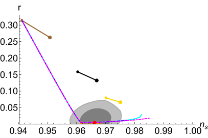
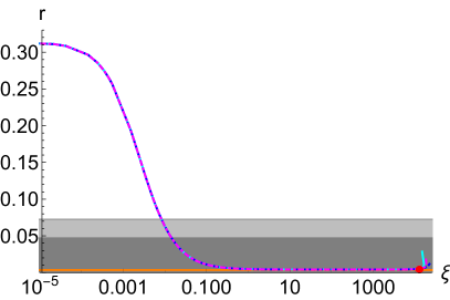
a)                                                             b)

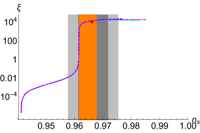
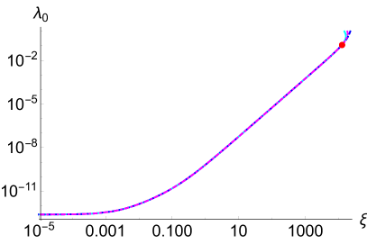
c)                                                             d)

Figure 1: Metric formulation: $r$ vs. $n_{s}$ (a), $r$ vs. $\xi$ (b), $\xi$ vs. $n_{s}$ (c) and $\lambda_{0}$ vs. $\xi$ (d) for $\lambda_{\rm eff}=\lambda_{\rm app}$ (cyan), $\lambda_{\rm eff}=\lambda_{\rm I}$ (blue, dashed) and $\lambda_{\rm eff}=\lambda_{\rm II}$ (magenta, dot-dashed) with $N_{e}=50$ $e$-folds. The red point indicates the loss of accuracy of the present analysis. For reference we also plot predictions of quartic (brown), quadratic (black) and linear (yellow) inflation for $N_{e}\in[50,60]$. The gray areas represent the 1,2$\sigma$ allowed regions coming from Planck 2018 data Planck2018:inflation .

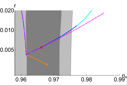
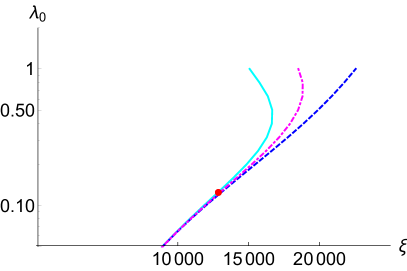
a)                                                             b)

Figure 2: Metric formulation: zoom of $r$ vs. $n_{s}$ (a) for $r\leq 0.02$ and $\lambda$ vs. $\xi$ (b) for $\lambda_{0}\geq 0.05$. The color code is the same as in Fig. 1.

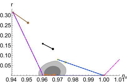
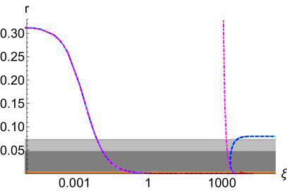
a)                                                             b)

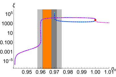
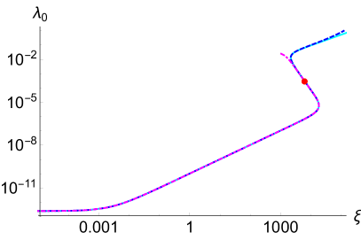
c)                                                             d)

Figure 3: Palatini formulation: $r$ vs. $n_{s}$ (a), $r$ vs. $\xi$ (b), $\xi$ vs. $n_{s}$ (c) and $\lambda_{0}$ vs. $\xi$ (d) for $\lambda_{\rm eff}=\lambda_{\rm app}$ (cyan), $\lambda_{\rm eff}=\lambda_{\rm I}$ (blue, dashed) and $\lambda_{\rm eff}=\lambda_{\rm II}$ (magenta, dot-dashed) with $N_{e}=50$ $e$-folds. The red point indicates the loss of accuracy of the present analysis. For reference we also plot predictions of quartic (brown), quadratic (black) and linear (yellow) inflation for $N_{e}\in[50,60]$. The gray areas represent the 1,2$\sigma$ allowed regions coming from Planck 2018 data Planck2018:inflation .

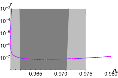
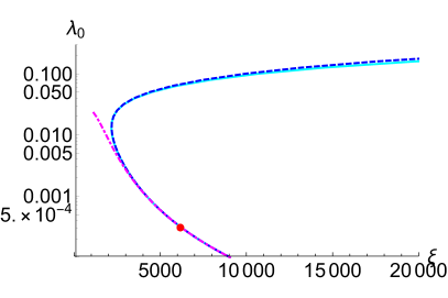
a)                                                             b)

Figure 4: Palatini formulation: zoom of $r$ vs. $n_{s}$ (a) for $r\leq 10^{-3}$ and $\lambda_{0}$ vs. $\xi$ (b) for $\lambda_{0}\leq 0.3$. The color code is the same as in Fig. 3.

On the other hand, there are several differences between the results of the two formulations. First of all, while in the Palatini formulation it is possible to reach the linear inflation limit Racioppi:2018zoy within perturbativity, this never happens in case of metric gravity. The same happens for the strong coupling limit of $\lambda_{\rm eff}=\lambda_{\rm II}$, which is only allowed in Palatini gravity. Moreover, the lower limit for $r$ in the metric case coincides with the prediction of $R^{2}$ inflation, where quantum corrections are still sub-dominant, while for the Palatini case the lower limit is $r\gtrsim 10^{-7}$, where the loop effects are relevant. Furthermore, only in the Palatini formulation for $\lambda_{\rm eff}=\lambda_{\rm II}$ with $\lambda_{0}\gtrsim 0.03$ we encountered Landau poles in the inflationary region and therefore removed the corresponding points. In addition, comparing Figs. 1 and 3 we can see that while in the metric case $\xi$ is monotonically increasing with $\lambda_{0}$, in the Palatini one $\xi$ increases until $n_{s}\sim 1$ is reached, then it decreases, and then it increases again. In the first and third region $\xi$ behaves as expected, therefore let us focus on the region $n_{s}\lesssim 1$, where there results of $\lambda_{0}$ vs. $\xi$ were unforeseen. As shown in Fig. 3d, in this region the lines of $\lambda_{\rm eff}=\lambda_{\rm app,I,II}$ are still overlapped, therefore it is enough to study the $\lambda_{\rm eff}=\lambda_{\rm app}$ case. In such a region we can still apply the strong coupling limit $\xi\to\infty$ and approximate the Einstein frame potential again as a running cosmological constant (see eq. (29)). However now it is convenient to solve the field redefinition (18) as follows

$$\chi\simeq\frac{M_{\text{P}}}{\sqrt{\xi}}\left[\frac{1}{2}\ln\left(\frac{3\lambda_{0}}{4\xi}\right)+\ln\left(\frac{2\sqrt{\xi}\phi}{M_{\text{P}}}\right)\right]$$ (37)

where we conveniently shifted the position of $\chi=0$. Therefore the Einstein frame potential becomes

$$U(\chi)\simeq\frac{\lambda_{0}M_{\text{P}}^{4}}{4\xi^{2}}\left(1+\frac{9\lambda_{0}\sqrt{\xi}\chi}{8\pi^{2}M_{\text{P}}}\right)\,.$$ (38)

It can proven that in this case $\frac{9\lambda_{0}\sqrt{\xi}\chi}{8\pi^{2}M_{\text{P}}}\ll 1$ and therefore we can get the following approximated results

$$r\simeq r_{0}\left(1-\frac{r_{0}}{4}N_{e}\right)\,,\quad n_{s}\simeq 1-\frac{3}{8}r\,,$$ (39)

where $r_{0}$ is the tensor-to-scalar ratio computed at the lowest order

$$r_{0}=\frac{81\xi}{8\pi^{4}}\lambda_{0}^{2}\,.$$ (40)

The constraint on the amplitude of the perturbation (22) implies

$$A_{s}\simeq\frac{4\pi^{2}}{243\lambda_{0}\xi^{3}}+\frac{\lambda_{0}N_{e}}{16\pi^{2}\xi^{2}}\,.$$ (41)

Now considering the small $\lambda_{0}$ limit, we get

$$A_{s}\simeq\frac{4\pi^{2}}{243\lambda_{0}\xi^{3}}\,,$$ (42)

and consequently

$$r_{0}\simeq\frac{2}{729}\frac{1}{A_{s}^{2}\,\xi^{5}}\,.$$ (43)

Henceforth, inserting eq. (43) into eq. (39), we find that, for big enough $\xi$, $r\simeq 0$ and $n_{s}\simeq 1$. Moreover, from eq. (42) we can see that $\lambda_{0}$ is inversely proportional to $\xi^{3}$. These results are in agreement with our numerical ones for $\lambda_{\rm eff}=\lambda_{\rm app}$ when $n_{s}\simeq 1$ in the Palatini formulation. On the other hand it is also interesting to see separately the corresponding limit of the Einstein frame potential for $\lambda_{\rm eff}=\lambda_{\rm II}$. Such limit is already given in eq. (34) and the consequent constraint on the amplitude is

$$A_{s}\simeq\frac{4\pi^{2}}{243\lambda_{0}\xi^{3}}-\frac{\lambda_{0}N_{e}}{48\pi^{2}\xi^{2}}\,,$$ (44)

which recovers the results of $\lambda_{\rm eff}=\lambda_{\rm app}$ for small $\lambda_{0}$ and departs from them by increasing $\lambda_{0}$ and allowing the possibility of $n_{s}\gtrsim 1$ (see eq. (36)). Therefore, in the Palatini formulation it is possible to discriminate between $\lambda_{\rm eff}=\lambda_{\rm I,II}$ far away from the 2$\sigma$ allowed region, nearby $n_{s}\sim 1$ ($\lambda_{0}\gtrsim 0.005$) (represented by the red point in Figs. 3 and 4). On the other hand, in the metric case it is impossible to discriminate between $\lambda_{\rm eff}=\lambda_{\rm I,II}$ within the 1$\sigma$ region, but it is possible within the 2$\sigma$ boundary from $\lambda_{0}\gtrsim 0.15$ $(\xi\gtrsim 1.4\times 10^{4})$ (represented by the red point in Figs. 1 and 2). As we mentioned before, there should be no physical difference in $\lambda_{\rm eff}=\lambda_{\rm I,II}$, therefore this should be interpreted as a loss of accuracy in the expansion for the effective potential in eq. (4) and the need to consider higher order loop corrections.

Finally we conclude remarking that, in agreement with the findings of Jinno:2019und , the impact of radiative corrections is stronger in the Palatini formulation rather than in the metric formulation, because the Jordan frame field excursion is larger in the Palatini formulation.

5 Conclusions

Even though we might expect the presence of multiple scalar fields at high energies which will affect the phenomenology, for instance, by inducing multi-field inflationary scenarios (e.g. Kaiser:2013sna ; Kallosh:2013daa ; Kuusk:2015dda ; Carrilho:2018ffi and refs therein) and/or relevant non-gaussianities (e.g. Seery:2005gb and refs therein), single field models of inflation are attractive for their simplicity and predictivity.

In particular, in this article we studied a model of quartic inflation where the inflaton field $\phi$ is subject to relevant self-induced radiative corrections and it is coupled non-minimally to gravity. We considered the Higgs-inflation-like non-minimal coupling. We studied the predictions of two different formulations of gravity, metric or Palatini, and the three possible versions of the effective quartic couplings $\lambda_{\rm eff}(\phi,\mu)=\lambda_{\rm app,I,II}(\phi)$: $\lambda_{\rm app}$ is the case in which the tree-level quartic coupling $\lambda_{0}$ is very small, we can Taylor expand and explicitly remove from $\lambda_{\rm eff}$ the dependence on the renormalization scale $\mu$, while $\lambda_{\rm eff}(\phi,\mu)=\lambda_{\rm I,II}(\phi)$ corresponds to the prescription I,II choices given in eqs. (8) and (9). We showed that the formulations share several differences, as expected, but also some interesting similarities. We start with the last ones.

First of all, trivially, the predictions are compatible with the ones of standard quartic inflation for $\xi\simeq 0$. Then, by increasing $\xi$ until $\xi\lesssim 10^{3}$, the predictions are substantially the same as the respective strong-coupling limits of the standard (tree-level) non-minimal inflation (Kallosh:2013tua for metric and Jarv:2017azx for Palatini). When $\lambda_{0}\lesssim 0.1$ $(\xi\lesssim 1.2\times 10^{4})$ in metric gravity, the predictions for $\lambda_{\rm eff}=\lambda_{\rm app,I,II}$ are undistinguishable. The same holds for $\lambda_{0}\lesssim 10^{-3}$ $(\xi\lesssim 4\times 10^{3})$ in Palatini gravity. Moreover, we showed that for $\xi\gg 1$, $\lambda_{\rm app}$ and $\lambda_{\rm I}$ can be mapped into each other just by varying $\lambda_{0}$ and $\xi$. Therefore it is impossible to distinguish between $\lambda_{\rm eff}=\lambda_{\rm app,I}$ in the $r$ vs. $n_{s}$ plots respectively in both gravity formulations. Eventual differences are appreciable only in the actual values of $\lambda_{0}$ and $\xi$.

On the other hand, the first difference that we notice is the possibility to reach within perturbativity the linear inflation limit Racioppi:2018zoy or the strong coupling limit (34) of $\lambda_{\rm II}$ only in Palatini gravity. Moreover, the lower limit for $r$ in the metric case coincides with the prediction of Starobinsky inflation, while for the Palatini case the lower limit is $r\gtrsim 10^{-7}$. In the metric case $\xi$ is everywhere monotonically increasing with $\lambda_{0}$, while in the Palatini one $\xi$ can also decrease around the value $n_{s}\simeq 1$. Around such a value, still in Palatini gravity, it is also possible to discriminate between $\lambda_{\rm eff}=\lambda_{\rm I,II}$ for $\lambda_{0}\gtrsim 0.005$. On the other hand, in the metric case it is impossible to discriminate between $\lambda_{\rm eff}=\lambda_{\rm I,II}$ within the 1$\sigma$ region, but it is possible within the 2$\sigma$ boundary from $\lambda_{0}\gtrsim 0.15$ $(\xi\gtrsim 1.4\times 10^{4})$. As there should be no physical difference in $\lambda_{\rm eff}=\lambda_{\rm I,II}$, this should point out a loss of accuracy in the expansion for the effective potential in eq. (4) and the need to add higher order loop corrections. This will be considered in a separate work.

Appendix A More details about the running of $\xi$

In this Appendix we present more details about the running of the non-minimal coupling to gravity in both the metric and the Palatini formulations. We start with the metric case and reminding the corresponding tree-level action

$$S=\!\!\int\!\!d^{4}x\sqrt{-g}\left(-\frac{M_{P}^{2}}{2}f(\phi)R(\bar{\Gamma})+\frac{(\partial\phi)^{2}}{2}-V(\phi)\right),$$ (45)

where

$$f(\phi) = 1+\xi\frac{\phi^{2}}{M_{P}^{2}}\,,$$ (46)

$$V(\phi) = \frac{1}{4}\lambda\phi^{4}\,,$$ (47)

and $\bar{\Gamma}$ is the Levi-Civita connection in eq. (11). The beta-function for $\xi$ is well known Buchbinder:1992rb

$$\beta_{\xi}=\frac{6\lambda}{16\pi^{2}}\left(\xi+\frac{1}{6}\right)\,.$$ (48)

Therefore it is easy to check that the running of $\xi$ is always negligible (i.e. $\frac{\beta_{\xi}}{\xi}\ll 1$) during the inflationary regime in the metric theory. When $\xi\ll 1$, we have

$$\frac{\beta_{\xi}}{\xi}\approx\frac{\lambda}{16\pi^{2}}<\frac{1}{16\pi^{2}}\ll 1\,,$$ (49)

while, when $\xi\approx O(1)$ or $\xi\gg 1$, we have

$$\frac{\beta_{\xi}}{\xi}\approx\frac{3\lambda}{8\pi^{2}}<\frac{3}{8\pi^{2}}\ll 1\,,$$ (50)

where we have used in both cases the pertubativity bound $\lambda<1$. Therefore, until the perturbativity is preserved, the running of $\xi$ can be ignored in the metric theory.

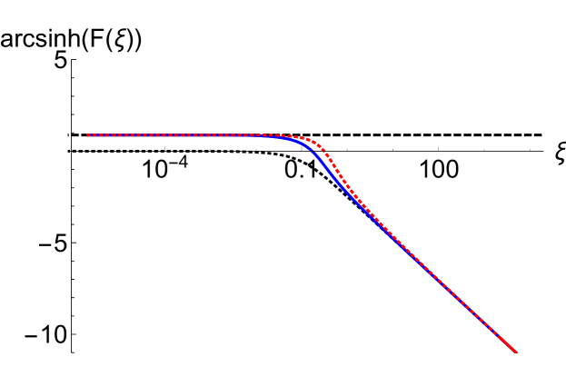
Figure 5: $\text{arcsinh}(F(\xi))$ with $F(\xi)=k(\phi_{f})$ (red, dotted), $F(\xi)=k(\phi_{N})$ (blue, continuous), $F(\xi)=1$ (black, dashed) and $F(\xi)=-6\xi$ (black, dotted).

Let us move now to the Palatini case. The corresponding action is the same as in eq. (45), but with replacement of $\bar{\Gamma}$ with $\Gamma$ given in eq. (12). However, it is possible to rewrite the Palatini action as the action of a non-minimally coupled metric theory with a non-minimal kinetic term Koivisto:2005yc , obtaining

$$S=\!\!\int\!\!d^{4}x\sqrt{-g}\left(-\frac{M_{P}^{2}}{2}f(\phi)R(\bar{\Gamma})+\frac{k(\phi)}{2}(\partial\phi)^{2}-V(\phi)\right)\,,$$ (51)

where the difference between the two formulations is now encoded in

$$k(\phi)=1-6\frac{\xi^{2}\phi^{2}}{{M_{\rm P}}^{2}+\xi\phi^{2}}\,.$$ (52)

Given the non-minimality of the kinetic term of the inflaton, an exhaustive computation of the radiative corrections (including the running of $\xi$) in the Palatini case is a task beyond the purpose of the present article. We can anyhow show a rather simple argument in support to our assumption of neglecting the contribution raising from $\beta_{\xi}$ also in the Palatini formulation. In order to do that, we plot in Fig. 5 $\text{arcsinh}(F(\xi))$ with $F(\xi)=k(\phi_{f})$ (red, dotted), $F(\xi)=k(\phi_{N})$ (blue, continuous), $F(\xi)=1$ (black, dashed) and $F(\xi)=-6\xi$ (black, dotted), where $\phi(\chi)$

$$\phi(\chi)=\frac{M_{P}}{\sqrt{\xi}}\sinh\left(\frac{\sqrt{\xi}\chi}{M_{P}}\right)$$ (53)

is computed by solving and then inverting eq. (18), $\phi_{f,N}=\phi(\chi_{f,N})$ and $\chi_{f,N}$ is defined after eq. (21). The choice of plotting the inverse hyperbolic sine is motivated by the need of a logarithmic scale on the $y$-axis for functions that also assume negative values. We can see that for most of the values of $\xi$ the non-minimal kinetic factors $k(\phi_{N,f})$ are either 1 or $-6\xi$. In the first case the computation is numerically equivalent to the usual metric case (cf. Figs. 1 and 3) and we have already shown before that the running of $\xi$ is negligible in this case. In the second case, $k(\phi_{N,f})\simeq-6\xi$, it is easy to check that the theory becomes conformal and therefore also in this case the running of $\xi$ is absent. To conclude we also notice that there is a small region around $\xi\approx 0.1-1$ where the $k(\phi_{N,f})$ is neither 1 nor $-6\xi$. In this case we can only make the reasonable guess that, considering the shape and continuity of the involved functions, the running of $\xi$ still remains irrelevant. Therefore, until the perturbativity of the theory is preserved, we ignore the running of $\xi$ also in the Palatini case.

References

- (1) A. A. Starobinsky, A New Type of Isotropic Cosmological Models Without Singularity, Phys. Lett. B91 (1980) 99.
- (2) A. H. Guth, The Inflationary Universe: A Possible Solution to the Horizon and Flatness Problems, Phys.Rev. D23 (1981) 347.
- (3) A. D. Linde, A New Inflationary Universe Scenario: A Possible Solution of the Horizon, Flatness, Homogeneity, Isotropy and Primordial Monopole Problems, Phys.Lett. B108 (1982) 389.
- (4) A. Albrecht and P. J. Steinhardt, Cosmology for Grand Unified Theories with Radiatively Induced Symmetry Breaking, Phys.Rev.Lett. 48 (1982) 1220.
- (5) BICEP2, Planck collaboration, Joint Analysis of BICEP2/ and Data, Phys. Rev. Lett. 114 (2015) 101301 [1502.00612].
- (6) Planck collaboration, Planck 2015 results. XIII. Cosmological parameters, Astron. Astrophys. 594 (2016) A13 [1502.01589].
- (7) Planck collaboration, Planck 2015 results. XX. Constraints on inflation, Astron. Astrophys. 594 (2016) A20 [1502.02114].
- (8) BICEP2, Keck Array collaboration, Improved Constraints on Cosmology and Foregrounds from BICEP2 and Keck Array Cosmic Microwave Background Data with Inclusion of 95 GHz Band, Phys. Rev. Lett. 116 (2016) 031302 [1510.09217].
- (9) Planck collaboration, Planck 2018 results. X. Constraints on inflation, 1807.06211.
- (10) T. Futamase and K.-i. Maeda, Chaotic Inflationary Scenario in Models Having Nonminimal Coupling With Curvature, Phys. Rev. D39 (1989) 399.
- (11) D. S. Salopek, J. R. Bond and J. M. Bardeen, Designing Density Fluctuation Spectra in Inflation, Phys. Rev. D40 (1989) 1753.
- (12) R. Fakir and W. G. Unruh, Improvement on cosmological chaotic inflation through nonminimal coupling, Phys. Rev. D41 (1990) 1783.
- (13) L. Amendola, M. Litterio and F. Occhionero, The Phase space view of inflation. 1: The nonminimally coupled scalar field, Int. J. Mod. Phys. A5 (1990) 3861.
- (14) D. I. Kaiser, Primordial spectral indices from generalized Einstein theories, Phys. Rev. D52 (1995) 4295 [astro-ph/9408044].
- (15) F. L. Bezrukov and M. Shaposhnikov, The Standard Model Higgs boson as the inflaton, Phys. Lett. B659 (2008) 703 [0710.3755].
- (16) S. C. Park and S. Yamaguchi, Inflation by non-minimal coupling, JCAP 0808 (2008) 009 [0801.1722].
- (17) A. Linde, M. Noorbala and A. Westphal, Observational consequences of chaotic inflation with nonminimal coupling to gravity, JCAP 1103 (2011) 013 [1101.2652].
- (18) D. I. Kaiser and E. I. Sfakianakis, Multifield Inflation after Planck: The Case for Nonminimal Couplings, Phys. Rev. Lett. 112 (2014) 011302 [1304.0363].
- (19) R. Kallosh and A. Linde, Non-minimal Inflationary Attractors, JCAP 1310 (2013) 033 [1307.7938].
- (20) R. Kallosh and A. Linde, Multi-field Conformal Cosmological Attractors, JCAP 1312 (2013) 006 [1309.2015].
- (21) R. Kallosh, A. Linde and D. Roest, Universal Attractor for Inflation at Strong Coupling, Phys. Rev. Lett. 112 (2014) 011303 [1310.3950].
- (22) M. Galante, R. Kallosh, A. Linde and D. Roest, Unity of Cosmological Inflation Attractors, Phys. Rev. Lett. 114 (2015) 141302 [1412.3797].
- (23) L. Järv, K. Kannike, L. Marzola, A. Racioppi, M. Raidal, M. Rünkla et al., Frame-Independent Classification of Single-Field Inflationary Models, Phys. Rev. Lett. 118 (2017) 151302 [1612.06863].
- (24) T. Chiba and K. Kohri, Consistency Relations for Large Field Inflation: Non-minimal Coupling, PTEP 2015 (2015) 023E01 [1411.7104].
- (25) L. Boubekeur, E. Giusarma, O. Mena and H. Ramírez, Does Current Data Prefer a Non-minimally Coupled Inflaton?, Phys. Rev. D91 (2015) 103004 [1502.05193].
- (26) M. Pieroni, -function formalism for inflationary models with a non minimal coupling with gravity, JCAP 1602 (2016) 012 [1510.03691].
- (27) A. Salvio, Inflationary Perturbations in No-Scale Theories, Eur. Phys. J. C77 (2017) 267 [1703.08012].
- (28) N. Bostan, Ö. Güleryüz and V. N. Şenoǧuz, Inflationary predictions of double-well, Coleman-Weinberg, and hilltop potentials with non-minimal coupling, JCAP 1805 (2018) 046 [1802.04160].
- (29) J. P. Beltrán Almeida and N. Bernal, Nonminimally coupled pseudoscalar inflaton, Phys. Rev. D98 (2018) 083519 [1803.09743].
- (30) W. Cheng and L. Bian, Higgs inflation and cosmological electroweak phase transition with N scalars in the post-Higgs era, Phys. Rev. D99 (2019) 035038 [1805.00199].
- (31) Y. Tang and Y.-L. Wu, Inflation in gauge theory of gravity with local scaling symmetry and quantum induced symmetry breaking, Phys. Lett. B784 (2018) 163 [1805.08507].
- (32) K. Sravan Kumar and P. Vargas Moniz, Conformal GUT inflation, proton lifetime and non-thermal leptogenesis, Eur. Phys. J. C79 (2019) 945 [1806.09032].
- (33) J. Kubo, M. Lindner, K. Schmitz and M. Yamada, Planck mass and inflation as consequences of dynamically broken scale invariance, Phys. Rev. D100 (2019) 015037 [1811.05950].
- (34) D. D. Canko, I. D. Gialamas and G. P. Kodaxis, A simple deformation of Starobinsky inflationary model, 1901.06296.
- (35) N. Okada and D. Raut, Hunting Inflaton at FASER, 1910.09663.
- (36) A. Karam, L. Marzola, T. Pappas, A. Racioppi and K. Tamvakis, Constant-Roll (Quasi-)Linear Inflation, JCAP 1805 (2018) 011 [1711.09861].
- (37) A. Karam, T. Pappas and K. Tamvakis, Nonminimal Coleman–Weinberg Inflation with an term, JCAP 1902 (2019) 006 [1810.12884].
- (38) N. D. Birrell and P. C. W. Davies, Quantum Fields in Curved Space, Cambridge Monographs on Mathematical Physics. Cambridge Univ. Press, Cambridge, UK, 1984, 10.1017/CBO9780511622632.
- (39) F. Bauer and D. A. Demir, Inflation with Non-Minimal Coupling: Metric versus Palatini Formulations, Phys. Lett. B665 (2008) 222 [0803.2664].
- (40) F. Bauer and D. A. Demir, Higgs-Palatini Inflation and Unitarity, Phys. Lett. B698 (2011) 425 [1012.2900].
- (41) N. Tamanini and C. R. Contaldi, Inflationary Perturbations in Palatini Generalised Gravity, Phys. Rev. D83 (2011) 044018 [1010.0689].
- (42) T. Tenkanen, Resurrecting Quadratic Inflation with a non-minimal coupling to gravity, JCAP 1712 (2017) 001 [1710.02758].
- (43) L. Järv, A. Racioppi and T. Tenkanen, The Palatini side of inflationary attractors, 1712.08471.
- (44) S. Rasanen, Higgs inflation in the Palatini formulation with kinetic terms for the metric, 1811.09514.
- (45) P. Carrilho, D. Mulryne, J. Ronayne and T. Tenkanen, Attractor Behaviour in Multifield Inflation, JCAP 1806 (2018) 032 [1804.10489].
- (46) J. P. B. Almeida, N. Bernal, J. Rubio and T. Tenkanen, Hidden Inflaton Dark Matter, JCAP 1903 (2019) 012 [1811.09640].
- (47) T. Takahashi and T. Tenkanen, Towards distinguishing variants of non-minimal inflation, JCAP 1904 (2019) 035 [1812.08492].
- (48) I. Antoniadis, A. Karam, A. Lykkas, T. Pappas and K. Tamvakis, Rescuing Quartic and Natural Inflation in the Palatini Formalism, JCAP 1903 (2019) 005 [1812.00847].
- (49) T. Tenkanen, Minimal Higgs inflation with an term in Palatini gravity, Phys. Rev. D99 (2019) 063528 [1901.01794].
- (50) T. Tenkanen and L. Visinelli, Axion dark matter from Higgs inflation with an intermediate , JCAP 1908 (2019) 033 [1906.11837].
- (51) T. Tenkanen, Trans-Planckian Censorship, Inflation and Dark Matter, 1910.00521.
- (52) N. Bostan, Quadratic, Higgs and hilltop potentials in the Palatini gravity, 1908.09674.
- (53) I. D. Gialamas and A. B. Lahanas, Reheating in Palatini inflationary models, 1911.11513.
- (54) S. Rasanen and P. Wahlman, Higgs inflation with loop corrections in the Palatini formulation, JCAP 1711 (2017) 047 [1709.07853].
- (55) K. Kannike, A. Kubarski, L. Marzola and A. Racioppi, A minimal model of inflation and dark radiation, Phys. Lett. B792 (2019) 74 [1810.12689].
- (56) V.-M. Enckell, K. Enqvist, S. Rasanen and E. Tomberg, Higgs inflation at the hilltop, JCAP 1806 (2018) 005 [1802.09299].
- (57) A. Racioppi, Coleman-Weinberg linear inflation: metric vs. Palatini formulation, JCAP 1712 (2017) 041 [1710.04853].
- (58) A. Racioppi, New universal attractor in nonminimally coupled gravity: Linear inflation, Phys. Rev. D97 (2018) 123514 [1801.08810].
- (59) I. Antoniadis, A. Karam, A. Lykkas and K. Tamvakis, Palatini inflation in models with an term, JCAP 1811 (2018) 028 [1810.10418].
- (60) N. Bostan, Non-minimally coupled quartic inflation with Coleman-Weinberg one-loop corrections in the Palatini formulation, 1907.13235.
- (61) T. Markkanen, T. Tenkanen, V. Vaskonen and H. Veermäe, Quantum corrections to quartic inflation with a non-minimal coupling: metric vs. Palatini, 1712.04874.
- (62) V.-M. Enckell, K. Enqvist, S. Rasanen and L.-P. Wahlman, Inflation with term in the Palatini formalism, JCAP 1902 (2019) 022 [1810.05536].
- (63) A. Kozak and A. Borowiec, Palatini frames in scalar-tensor theories of gravity, Eur. Phys. J. C79 (2019) 335 [1808.05598].
- (64) K. Kannike, A. Racioppi and M. Raidal, Embedding inflation into the Standard Model - more evidence for classical scale invariance, JHEP 06 (2014) 154 [1405.3987].
- (65) L. Marzola, A. Racioppi, M. Raidal, F. R. Urban and H. Veermäe, Non-minimal CW inflation, electroweak symmetry breaking and the 750 GeV anomaly, JHEP 03 (2016) 190 [1512.09136].
- (66) L. Marzola and A. Racioppi, Minimal but non-minimal inflation and electroweak symmetry breaking, JCAP 1610 (2016) 010 [1606.06887].
- (67) K. Dimopoulos, C. Owen and A. Racioppi, Loop inflection-point inflation, Astropart. Phys. 103 (2018) 16 [1706.09735].
- (68) K. Kannike, G. Hütsi, L. Pizza, A. Racioppi, M. Raidal, A. Salvio et al., Dynamically Induced Planck Scale and Inflation, JHEP 05 (2015) 065 [1502.01334].
- (69) K. Kannike, A. Racioppi and M. Raidal, Linear inflation from quartic potential, JHEP 01 (2016) 035 [1509.05423].
- (70) A. Farzinnia and S. Kouwn, Classically scale invariant inflation, supermassive WIMPs, and adimensional gravity, Phys. Rev. D93 (2016) 063528 [1512.05890].
- (71) K. Kannike, A. Racioppi and M. Raidal, Super-heavy dark matter - Towards predictive scenarios from inflation, Nucl. Phys. B918 (2017) 162 [1605.09378].
- (72) M. Rinaldi, L. Vanzo, S. Zerbini and G. Venturi, Inflationary quasiscale-invariant attractors, Phys. Rev. D93 (2016) 024040 [1505.03386].
- (73) N. D. Barrie, A. Kobakhidze and S. Liang, Natural Inflation with Hidden Scale Invariance, Phys. Lett. B756 (2016) 390 [1602.04901].
- (74) M. Artymowski and A. Racioppi, Scalar-tensor linear inflation, JCAP 1704 (2017) 007 [1610.09120].
- (75) I. Buchbinder, S. Odintsov and I. Shapiro, Effective action in quantum gravity. 1992.
- (76) E. Elizalde and S. D. Odintsov, Renormalization group improved effective Lagrangian for interacting theories in curved space-time, Phys. Lett. B321 (1994) 199 [hep-th/9311087].
- (77) T. Inagaki, R. Nakanishi and S. D. Odintsov, Non-Minimal Two-Loop Inflation, Phys. Lett. B745 (2015) 105 [1502.06301].
- (78) D. P. George, S. Mooij and M. Postma, Quantum corrections in Higgs inflation: the real scalar case, JCAP 1402 (2014) 024 [1310.2157].
- (79) T. Prokopec and J. Weenink, Frame independent cosmological perturbations, JCAP 1309 (2013) 027 [1304.6737].
- (80) L. Järv, P. Kuusk, M. Saal and O. Vilson, Invariant quantities in the scalar-tensor theories of gravitation, Phys. Rev. D91 (2015) 024041 [1411.1947].
- (81) P. Kuusk, L. Järv and O. Vilson, Invariant quantities in the multiscalar-tensor theories of gravitation, Int. J. Mod. Phys. A31 (2016) 1641003 [1509.02903].
- (82) P. Kuusk, M. Rünkla, M. Saal and O. Vilson, Invariant slow-roll parameters in scalar-tensor theories, Class. Quant. Grav. 33 (2016) 195008 [1605.07033].
- (83) E. E. Flanagan, The Conformal frame freedom in theories of gravitation, Class. Quant. Grav. 21 (2004) 3817 [gr-qc/0403063].
- (84) R. Catena, M. Pietroni and L. Scarabello, Einstein and Jordan reconciled: a frame-invariant approach to scalar-tensor cosmology, Phys. Rev. D76 (2007) 084039 [astro-ph/0604492].
- (85) A. O. Barvinsky, A. Yu. Kamenshchik and A. A. Starobinsky, Inflation scenario via the Standard Model Higgs boson and LHC, JCAP 0811 (2008) 021 [0809.2104].
- (86) A. De Simone, M. P. Hertzberg and F. Wilczek, Running Inflation in the Standard Model, Phys. Lett. B678 (2009) 1 [0812.4946].
- (87) A. O. Barvinsky, A. Yu. Kamenshchik, C. Kiefer, A. A. Starobinsky and C. Steinwachs, Asymptotic freedom in inflationary cosmology with a non-minimally coupled Higgs field, JCAP 0912 (2009) 003 [0904.1698].
- (88) A. O. Barvinsky, A. Yu. Kamenshchik, C. Kiefer, A. A. Starobinsky and C. F. Steinwachs, Higgs boson, renormalization group, and naturalness in cosmology, Eur. Phys. J. C72 (2012) 2219 [0910.1041].
- (89) C. F. Steinwachs and A. Yu. Kamenshchik, One-loop divergences for gravity non-minimally coupled to a multiplet of scalar fields: calculation in the Jordan frame. I. The main results, Phys. Rev. D84 (2011) 024026 [1101.5047].
- (90) T. Chiba and M. Yamaguchi, Conformal-Frame (In)dependence of Cosmological Observations in Scalar-Tensor Theory, JCAP 1310 (2013) 040 [1308.1142].
- (91) M. Postma and M. Volponi, Equivalence of the Einstein and Jordan frames, Phys. Rev. D90 (2014) 103516 [1407.6874].
- (92) A. Yu. Kamenshchik and C. F. Steinwachs, Question of quantum equivalence between Jordan frame and Einstein frame, Phys. Rev. D91 (2015) 084033 [1408.5769].
- (93) D. P. George, S. Mooij and M. Postma, Quantum corrections in Higgs inflation: the Standard Model case, JCAP 1604 (2016) 006 [1508.04660].
- (94) S. P. Miao and R. P. Woodard, Fine Tuning May Not Be Enough, JCAP 1509 (2015) 022 [1506.07306].
- (95) E. Elizalde and S. D. Odintsov, Renormalization group improved effective potential for gauge theories in curved space-time, Phys. Lett. B303 (1993) 240 [hep-th/9302074].
- (96) E. Elizalde and S. D. Odintsov, Renormalization group improved effective potential for finite grand unified theories in curved space-time, Phys. Lett. B333 (1994) 331 [hep-th/9403132].
- (97) D. Burns, S. Karamitsos and A. Pilaftsis, Frame-Covariant Formulation of Inflation in Scalar-Curvature Theories, Nucl. Phys. B907 (2016) 785 [1603.03730].
- (98) J. Fumagalli and M. Postma, UV (in)sensitivity of Higgs inflation, JHEP 05 (2016) 049 [1602.07234].
- (99) J. Fumagalli, Renormalization Group independence of Cosmological Attractors, Phys. Lett. B769 (2017) 451 [1611.04997].
- (100) F. Bezrukov, M. Pauly and J. Rubio, On the robustness of the primordial power spectrum in renormalized Higgs inflation, 1706.05007.
- (101) A. Karam, T. Pappas and K. Tamvakis, Frame-dependence of higher-order inflationary observables in scalar-tensor theories, Phys. Rev. D96 (2017) 064036 [1707.00984].
- (102) G. Narain, On the renormalization group perspective of -attractors, JCAP 1710 (2017) 032 [1708.00830].
- (103) M. S. Ruf and C. F. Steinwachs, Quantum equivalence of -gravity and scalar-tensor-theories, 1711.07486.
- (104) T. Markkanen, S. Nurmi, A. Rajantie and S. Stopyra, The 1-loop effective potential for the Standard Model in curved spacetime, JHEP 06 (2018) 040 [1804.02020].
- (105) N. Ohta, Quantum equivalence of gravity and scalar-tensor theories in the Jordan and Einstein frames, PTEP 2018 (2018) 033B02 [1712.05175].
- (106) P. G. Ferreira, C. T. Hill and G. G. Ross, Inertial Spontaneous Symmetry Breaking and Quantum Scale Invariance, 1801.07676.
- (107) A. Karam, A. Lykkas and K. Tamvakis, Frame-invariant approach to higher-dimensional scalar-tensor gravity, Phys. Rev. D97 (2018) 124036 [1803.04960].
- (108) S. R. Coleman and E. J. Weinberg, Radiative Corrections as the Origin of Spontaneous Symmetry Breaking, Phys. Rev. D7 (1973) 1888.
- (109) C. G. Callan, Broken scale invariance in scalar field theory, Phys. Rev. D 2 (1970) 1541.
- (110) K. Symanzik, Small distance behaviour in field theory and power counting, Communications in Mathematical Physics 18 (1970) 227.
- (111) M. Neubert, Les Houches Lectures on Renormalization Theory and Effective Field Theories, in Les Houches summer school: EFT in Particle Physics and Cosmology Les Houches, Chamonix Valley, France, July 3-28, 2017, 2019, 1901.06573.
- (112) F. Bezrukov, The Higgs field as an inflaton, Class. Quant. Grav. 30 (2013) 214001 [1307.0708].
- (113) K. Allison, Higgs xi-inflation for the 125-126 GeV Higgs: a two-loop analysis, JHEP 02 (2014) 040 [1306.6931].
- (114) Y. Hamada, H. Kawai, Y. Nakanishi and K.-y. Oda, Meaning of the field dependence of the renormalization scale in Higgs inflation, Phys. Rev. D95 (2017) 103524 [1610.05885].
- (115) N. Bostan and V. N. Şenoǧuz, Quartic inflation and radiative corrections with non-minimal coupling, JCAP 1910 (2019) 028 [1907.06215].
- (116) F. Bezrukov, G. K. Karananas, J. Rubio and M. Shaposhnikov, Higgs-Dilaton Cosmology: an effective field theory approach, Phys. Rev. D87 (2013) 096001 [1212.4148].
- (117) R. Jinno, M. Kubota, K.-y. Oda and S. C. Park, Higgs inflation in metric and Palatini formalisms: Required suppression of higher dimensional operators, 1904.05699.
- (118) D. Seery and J. E. Lidsey, Primordial non-Gaussianities from multiple-field inflation, JCAP 09 (2005) 011 [astro-ph/0506056].
- (119) T. Koivisto and H. Kurki-Suonio, Cosmological perturbations in the palatini formulation of modified gravity, Class. Quant. Grav. 23 (2006) 2355 [astro-ph/0509422].