A Data-Centric Approach to Extreme-Scale Ab initio Dissipative Quantum Transport Simulations

Abstract.

The computational efficiency of a state of the art ab initio quantum transport (QT) solver, capable of revealing the coupled electro-thermal properties of atomically-resolved nano-transistors, has been improved by up to two orders of magnitude through a data centric reorganization of the application. The approach yields coarse-and fine-grained data-movement characteristics that can be used for performance and communication modeling, communication-avoidance, and dataflow transformations. The resulting code has been tuned for two top-6 hybrid supercomputers, reaching a sustained performance of 85.45 Pflop/s on 4,560 nodes of Summit (42.55% of the peak) in double precision, and 90.89 Pflop/s in mixed precision. These computational achievements enable the restructured QT simulator to treat realistic nanoelectronic devices made of more than 10,000 atoms within a 14$\times$ shorter duration than the original code needs to handle a system with 1,000 atoms, on the same number of CPUs/GPUs and with the same physical accuracy.

1. Justification for Prize

Record ab initio dissipative quantum transport simulation in devices made of $\geq$10,000 atoms (10$\times$ improvement w.r.t. state-of-the-art). Double precision performance of 85.45 Pflop/s on 4,560 nodes of Summit (27,360 GPUs), and mixed precision of 90.89 Pflop/s. Reduction in time-to-solution per atom and communication volume by a factor of up to 140 and 136, respectively.

2. Performance Attributes

Performance attribute	Our submission
Category of achievement	Scalability, time-to-solution
Type of method used	Non-linear system of equations
Results reported on basis of	Whole application including I/O
Precision reported	Double precision, Mixed precision
System scale	Measured on full-scale
Measurements	Timers, FLOP count, performance modeling

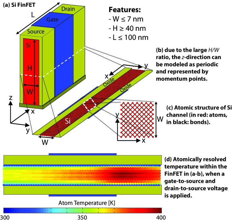
Figure 1. Self-heating effect simulation in a Silicon FinFET.

3. Overview of the Problem

Much of human technological development and scientific advances in the last decades have been driven by increases in computational power. The cost-neutral growth provided by Moore’s scaling law is however coming to an end, threatening to stall progress in strategic fields ranging from scientific simulations and bioinformatics to machine learning and the Internet-of-Things. All these areas share an insatiable need for compute power, which in turn drives much of their innovation. Future improvement of these fields, and science in general, will depend on overcoming fundamental technology barriers, one of which is the soon-to-become unmanageable heat dissipation in compute units.

Heat dissipation in microchips reached alarming peak values of 100 W/cm² already in 2006 (Wei, 2008; Pop et al., 2006). This led to the end of Dennard scaling and the beginning of the “multicore crisis”, an era with energy-efficient parallel, but sequentially slower multicore CPUs. Now, more than ten years later, average power densities of up to 30 W/cm², about four times more than hot plates, are commonplace in modern high-performance CPUs, putting thermal management at the center of attention of circuit designers (Pawlik, 2016). By scaling the dimensions of transistors more rapidly than their supply voltage, the semiconductor industry has kept increasing heat dissipation from one generation of microprocessors to the other. In this context, large-scale data and supercomputing centers are facing critical challenges regarding the design and cost of their cooling infrastructures. The price to pay for that has become exorbitant, as the cooling can consume up to 40% of the total electricity in data centers; a cumulative cost of many billion dollars per year.

Landauer’s theoretical limit of energy consumption for non-reversible computing offers a glimmer of hope: today’s processing units require orders of magnitude more energy than the $k_{B}T\ln 2$ Joule bound to (irreversibly) change one single bit. However, to approach this limit, it will be necessary to first properly understand the mechanisms behind nanoscale heat dissipation in semiconductor devices (Pop et al., 2006). Fin field-effect transistors (FinFETs), as schematized in Fig. 1(a-c), build the core of all recent integrated circuits (ICs). Their dimensions do not exceed 100 nanometers along all directions, even 10 nm along one of them (width $W$), with an active region composed of fewer than 1 million atoms. This makes them subject to strong quantum mechanical and peculiar thermal effects.

When a voltage $V_{ds}$ is applied across FinFETs, electrons start to flow from the source to the drain contact, giving rise to an electrical current whose magnitude depends on the gate bias $V_{gs}$. The potential difference between source and drain allows electrons to transfer part of their energy to the crystal lattice surrounding them. This energy is converted into atomic vibrations, called phonons, that can propagate throughout FinFETs. The more atoms vibrate, the “hotter” a device becomes. This phenomenon, known as self- or Joule-heating, plays a detrimental role in today’s transistor technologies and has consequences up to the system level. It is illustrated in Fig. 1(d) (§ 8.1 for details about this simulation): a strong increase of the lattice temperature can be observed close to the drain contact of the simulated FinFET. The negative influence of self-heating on CPU/GPU performance can be minimized by devising computer-assisted strategies to efficiently evacuate the generated heat from the active region of transistors.

3.1. Physical Model

Due to the large height/width ratio of FinFETs, heat generation and dissipation can be physically captured in a two-dimensional simulation domain comprising 10-15 thousand atoms and corresponding to a slice in the $x$-$y$ plane. The height, aligned with the $z$-axis (see Fig. 1(a-b)), can be treated as a periodic dimension and represented by a momentum vector $k_{z}$ or $q_{z}$ in the range $[-\pi,\pi]$. The tiny width ($W\leq$7 nm) and length $L\leq$100 nm) of such FinFETs require atomistic Quantum Transport (QT) simulation to accurately model and analyze their electro-thermal properties. In this framework, electron and phonon (thermal) currents as well as their interactions are evaluated by taking quantum mechanics into account.

The Non-equilibrium Green’s Function (NEGF) formalism (Datta, 1995) combined with density functional theory (DFT) (Kohn and Sham, 1965) lends itself optimally to this type of calculations including electron and phonon transport and thus to the investigation of self-heating in arbitrary device geometries. With the help of DFT, an ab initio method, any material (combination) can be handled at the atomic level without the need for empirical parameters.

The DFT+NEGF equations for electron and phonon transport take the form of a non-linear system of equations, as depicted in Fig. 2. The electron ($G(E,k_{z})$) and phonon ($D(\omega,q_{z})$) Green’s Functions (GF) at energy $E$, momentum $k_{z}$/$q_{z}$, and frequency $\omega$ are coupled to each other through scattering self-energies (SSE) $\Sigma(E,k_{z})$ and $\Pi(\omega,q_{z})$ that depend on $[G(E\pm\hbar\omega,k_{z}-q_{z})$ $D(\omega,q_{z})]$ and $[G(E,k_{z})$ $G(E+\hbar\omega,k_{z}+q_{z})]$, respectively.

The electron and phonon Green’s Functions are solved for all possible electron energy ($N_{E}$) and momentum ($N_{k_{z}}$) points as well as all phonon frequencies ($N_{\omega}$) and momentum ($N_{q_{z}}$). In case of self-heating, the difficulty does not come from the solution of the GF equations, which are independent from each other and have received a wide attention before (Luisier et al., 2011; Calderara et al., 2015), but from the fact that the scattering self-energies $\Sigma$ and $\Pi$ connect different energy-momentum ($E$, $k_{z}$) and frequency-momentum ($\omega$, $q_{z}$) pairs together.

To obtain the electrical and energy currents or the temperature distribution (see Fig. 1(d)) of a given device, the non-linear GF and SSE equations must be iteratively solved until convergence is reached. Depending on the geometry and bias conditions, between $N_{iter}$=20 and 100 iterations are needed for that. The algorithm starts by setting $\Sigma(E,k_{z})$=$\Pi(\omega,q_{z})$=0 and continues by computing all GFs under this condition. The latter then serve as inputs to the next phase, where the SSE are evaluated for all ($E$, $k_{z}$) and ($\omega$, $q_{z}$).

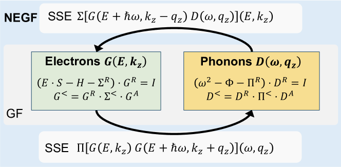
Figure 2. Self-consistent coupling between the GF and SSE phases (kernels) as part of the NEGF formalism.

Table 1. State of the Art Quantum Transport Simulators

Name	Maximum # of Computed Atoms						Scalability
	Tight-binding-like∗			DFT			Max. Cores	Using
	$GF^{\dagger}_{e}$	$GF^{\dagger}_{ph}$	$GF+SSE$	$GF^{\dagger}_{e}$	$GF^{\dagger}_{ph}$	$GF+SSE$	(Magnitude)	GPUs
GOLLUM (Ferrer et al., 2014)	1k	1k	—	100	100	—	N/A	✗
Kwant (Groth et al., 2014)	10k	—	—	—	—	—	N/A	✗
NanoTCAD ViDES (NanoTCAD, 2017)	10k	—	—	—	—	—	N/A	✗
QuantumATK (Synopsys, 2019)	10k	10k	—	1k	1k	—	1k	✗
TB_sim (Grenoble, 2013)	100k	—	10k‡	1k	—	—	10k	✓
NEMO5 (Group and Klimeck, 2018)	100k	100k	10k‡	—	—	—	100k	✓
OMEN (Luisier et al., 2006)	100k (1.44 Pflop/s (Luisier et al., 2011))	100k	10k	10k (15 Pflop/s (Calderara et al., 2015))	10k	1k (0.16 Pflop/s)	100k	✓
This work	N/A	N/A	N/A	10k	10k	10k (85.45 Pflop/s)	1M	✓

^∗: including Maximally-Localized Wannier Functions (MLWF), $\dagger$: Ballistic, $\ddagger$: Simplified.

3.2. Computational Challenges

An intuitive algorithm to practically solve the GF+SSE system on supercomputers consists of two loops: one over the momentum points ($k_{z}$/$q_{z}$) and another one over the electron energies ($E$). This loop schedule results in complex execution dependencies and communication patterns. The communication overhead quickly becomes a bottleneck with increasing number of atoms and computational resources, crossing the petabyte range per iteration for realistic transistor sizes (§ 6.1.2). Therefore, current simulations are limited to the order of 1,000 atoms, a value much below what is needed to apply QT simulations in practical applications.

Even in a scenario where each node operates at maximum computational efficiency, large-scale QT simulations are bound by both communication volume and memory requirements. The former inhibits strong scaling, as simulation time includes nanostructure-dependent point-to-point communication patterns, which become infeasible when increasing node count. The memory bottleneck is a direct result of the former. It hinders large simulations due to the increased memory requirements w.r.t. atom count. Transforming the QT simulation algorithm to minimize communication is thus the key to simultaneously model larger devices and increase scalability on different supercomputers.

4. Current State of the Art

Quantum transport simulation is an important driver of innovation in nanoelectronics. Thus, many atomistic quantum transport simulators that can model the characteristics of nano-devices have been developed (Ferrer et al., 2014; Groth et al., 2014; Group and Klimeck, 2018; Synopsys, 2019; NanoTCAD, 2017; Grenoble, 2013; Luisier et al., 2006). Their performance is summarized in Table 1, where their estimated maximum number of atoms that can be simulated for a given physical model is provided. Only orders of magnitude are shown, as these quantities depend on the device geometries and band-structure method. It should be mentioned that most tools are limited to tight-binding-like (TB) Hamiltonians, because they are computationally cheaper than DFT ones (less orbitals and neighbors per atom). This explains the larger systems that can be treated with TB. However, such approaches are not accurate enough when it comes to the exploration of material stacks, amorphous layers, metallic contacts, or interfaces as needed in transistor design. In these cases, the higher accuracy of DFT is required and leads to a much higher computational cost.

When it comes to the modeling of self-heating at the ab initio level, the following NEGF equations must be solved for electrons:

(3) $$\left\{\begin{array}[]{l}\left(E\cdot{\mathbf{S}}(k_{z})-{\mathbf{H}}(k_{z})-{\mathbf{\Sigma}}^{R}(E,k_{z})\right)\cdot{\mathbf{G}}^{R}(E,k_{z})={\mathbf{I}}\\ {\mathbf{G}}^{\gtrless}(E,k_{z})=\mathbf{G}^{R}(E,k_{z})\cdot{\mathbf{\Sigma}}^{\gtrless}(E,k_{z})\cdot{\mathbf{G}}^{A}(E,k_{z}).\end{array}\right.$$

In Eq. (3), ${\mathbf{S}}(k_{z})$ and ${\mathbf{H}}(k_{z})$ are the $k_{z}$-dependent overlap and Hamiltonian matrices, respectively. They must be produced by a DFT code with a localized basis set (here: CP2K (VandeVondele et al., 2005)) and have a size $N_{a}\times N_{orb}$ ($N_{a}$: total number of atoms, $N_{orb}$: number of orbitals per atom). The ${\mathbf{G}}(E,k_{z})$ electron GFs have the same size as ${\mathbf{S}/H}$ and ${\mathbf{I}}$, the identity matrix. They can be either retarded ($R$), advanced ($A$), lesser ($<$), or greater ($>$). The same notation applies to the self-energies ${\mathbf{\Sigma}}(E,k_{z})$ that include a boundary and scattering (superscript $S$) term.

To handle phonon transport, a similar GF system of equations must be processed: the electron energy $E$ is replaced by the square of the phonon frequency $\omega^{2}$, the Hamiltonian $H(k_{z})$ by the dynamical matrix ${\mathbf{\Phi}}(q_{z})$, and $S(k_{z})$ by the identity matrix $I$ with $N_{orb}$=$N_{3D}$=3, the three axes along which crystals can vibrate.

Eq. (3) and its phonon equivalent can be solved with a so-called recursive Green’s Function (RGF) algorithm (Svizhenko et al., 2002). All matrices ($H$, $S$, and $\Phi$) are block-tri-diagonal and can be divided into $bnum$ blocks with $\frac{N_{a}}{bnum}$ atoms each, if the structure is homogeneous, as here. RGF then performs a forward/backward pass over the $bnum$ blocks. It has been demonstrated that converting selected operations of RGF to single-precision typically leads to inaccurate results (Luisier et al., 2011).

The electron ($\Sigma^{S}$) and phonon ($\Pi^{S}$) scattering self-energies (less-er and greater components) can be written as follows (Stieger et al., 2017):

$${\mathbf{\Sigma}}^{\gtrless S}_{aa}(E,k_{z})=i\sum_{q_{z}ijl}\int\frac{d\hbar\omega}{2\pi}\left[\nabla_{i}{\mathbf{H}}_{ab}\cdot{\mathbf{G}}^{\gtrless}_{bb}(E-\hbar\omega,k_{z}-q_{z})\cdot\right.$$

$$\nabla_{j}{\mathbf{H}}_{ba}\cdot\left({\mathbf{D}}^{\gtrless ij}_{ba}(\omega,q_{z})-{\mathbf{D}}^{\gtrless ij}_{bb}(\omega,q_{z})-\right.$$

(4) $$\left.\left.{\mathbf{D}}^{\gtrless ij}_{aa}(\omega,q_{z})+{\mathbf{D}}^{\gtrless ij}_{ab}(\omega,q_{z})\right)\right],$$

(5) $${\mathbf{\Pi}}^{\gtrless S}_{ab}(\omega,q_{z})=-i\sum_{k_{z}l}\int\frac{dE}{2\pi}\mathrm{tr}\left\{\nabla_{i}{\mathbf{H}}_{la}\cdot{\mathbf{G}}^{\gtrless}_{aa}(E+\hbar\omega,k_{z}+q_{z})\cdot\right.$$

$$\left.\nabla_{j}{\mathbf{H}}_{al}\cdot{\mathbf{G}}^{\lessgtr}_{ll}(E,k_{z})\right\}.$$

In Eq. (5), the sum over $l$ is replaced by $l$=$b$, if $a$=$b$. All Green’s Functions ${\mathbf{G}_{ab}}$ (${\mathbf{D}_{ab}}$) are matrices of size $N_{orb}\times N_{orb}$ ($N_{3D}\times N_{3D}$). They describe the coupling between two neighbor atoms $a$ and $b$ at positions ${\mathbf{R}}_{a}$ and ${\mathbf{R}}_{b}$. Each atom has $N_{b}$ neighbors. The term $\nabla_{i}{\mathbf{H}}_{ab}$ is the derivative of the $\mathbf{H}_{ab}$ Hamiltonian coupling atoms $a$ and $b$. It is computed with DFT. Only the diagonal blocks of ${\mathbf{\Sigma}}^{R\gtrless,S}$ and $N_{b}$ non-diagonal blocks of ${\mathbf{\Pi}}^{R\gtrless,S}$ are considered.

The evaluation of Eqs. (4-5) does not require the knowledge of all entries of the ${\mathbf{G}}$ and ${\mathbf{D}}$ matrices, but of two 5-D tensors of shape $[N_{k_{z}},N_{E},N_{a},N_{orb},N_{orb}]$ for electrons and two 6-D tensors of shape $[N_{q_{z}},N_{\omega},N_{a},N_{b}+1,N_{3D},N_{3D}]$ for phonons. Each $[k_{z},E,N_{a},N_{orb},N_{orb}]$ and $[q_{z},\omega,N_{a},N_{b}+1,N_{3D},$ $N_{3D}]$ combination is produced independently from the other by solving the GF equations with RGF. The electron and phonon SSE can also be reshaped into multi-dimensional tensors with the same dimensions as their GF counterparts, but they cannot be computed independently due to energy, frequency, and momentum coupling.

To the best of our knowledge, the only tool that can solve Eqs. (3) to (5) self-consistently, in structures composed of thousands of atoms, at the DFT level is OMEN (Luisier et al., 2006), a two-time Gordon Bell Prize finalist (Luisier et al., 2011; Calderara et al., 2015). The application is written in C++, contains 90,000 lines of code in total, and uses MPI as its communication protocol. Some parts of it have been ported to GPUs using the CUDA language and take advantage of libraries such as cuBLAS, cuSPARSE, and MAGMA. The electron-phonon scattering model was first implemented based on the tight-binding method and a three-level MPI distribution of the workload (momentum, energy, and spatial domain decomposition). A first release of the model with equilibrium phonon (${\mathbf{\Pi}^{S}}$=0) was validated up to 95k cores for a device with $N_{a}$=5,402, $N_{b}$=4, $N_{orb}$=10, $N_{k_{z}}$=21, and $N_{E}$=1,130. These runs showed that the application can reach a parallel efficiency of 57%, when going from 3,276 up to 95,256 cores, with the SSE phase consuming from 25% to 50% of the total simulation times. The reason for the increase in SSE time could be attributed to the communication time required to gather all Green’s Function inputs for Eq. (4), which grew from 16 to 48% of the total simulation time (Luisier, 2010) as the number of cores went from 3,276 to 95,256.

After extending the electron-phonon scattering model to DFT and adding phonon transport to it, it has been observed that the time spent in the SSE phase (communication and computation) explodes. Even for a small structure with $N_{a}$=2,112, $N_{orb}$=4, $N_{k_{z}}$=$N_{q_{z}}$=11, $N_{E}$=650, $N_{\omega}$=30, and $N_{b}$=13, 95% of the total simulation time is dedicated to SSE, regardless of the number of used cores/nodes, among which $\sim$60% for the communication between the different MPI tasks. The relevance of this model is therefore limited.

Understanding realistic FinFET transistors requires simulations with $\mathbf{N_{a}\geq 10,000}$ atoms and high accuracy ($\mathbf{N_{k_{Z}}}$$\mathbf{>}$$\mathbf{20}$, $\mathbf{N_{E}}$$\mathbf{>}$$\mathbf{1,000}$, see Table 6). In order to achieve a reasonable cost (time, money, and energy), the algorithms to solve Eqs. (3) to (5) must be drastically improved. The required algorithmic improvements needed are at least one order of magnitude in the number of atoms and two orders of magnitude in computational time per atom. In the following sections, we demonstrate how both can be achieved with a novel data-centric view of the simulation.

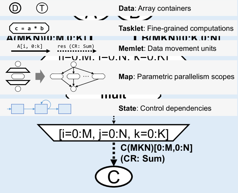
Figure 3. Stateful Dataflow Multigraph (SDFG) concepts.

5. Innovations Realized

The discussed self-heating effects have formed the landscape of current HPC systems, which consist of new architectures attempting to work around the physical constraints. Thus, no two cluster systems are the same and heterogeneity is commonplace. Each setup requires careful tuning of application performance, focused mostly on data movement, which causes the lion’s share of energy dissipation (Unat et al., 2017). As this kind of tuning demands in-depth knowledge of the hardware, it is typically performed by a  Performance Engineer, a developer who is versed in intricate system details, existing high-performance libraries, and capable of modeling performance and setting up optimized procedures independently. This role, which complements the  Domain Scientist, has been increasingly important in scientific computing for the past three decades, but is now essential for any application beyond straightforward linear algebra to operate at extreme scales. Until now, both Domain Scientists and Performance Engineers would work with one code-base. This creates a co-dependent  situation (P. McCormick, 2019), where the original domain code is tuned to a point that modifying the algorithm or transforming its behavior is difficult to one without the presence of the other, even if data locality or computational semantics are not changed.

Figure 4. SDFG of the entire simulation.

Figure 5. Requirements for Accurate
Dissipative DFT+NEGF Simulations

Variable	Description	Value
$N_{k_{z}}/N_{q_{z}}$	Number of electron/phonon momentum points	$\geq$21
$N_{E}$	Number of energy points	$\geq$1,000
$N_{\omega}$	Number of phonon frequencies	$\geq$50
$N_{a}$	Total number of atoms per device structure	$\geq$10,000
$N_{b}$	Neighbors considered for each atom	$\geq$30
$N_{orb}$	Number of orbitals per atom	$\geq$10
$N_{3D}$	Degrees of freedom for crystal vibrations	3

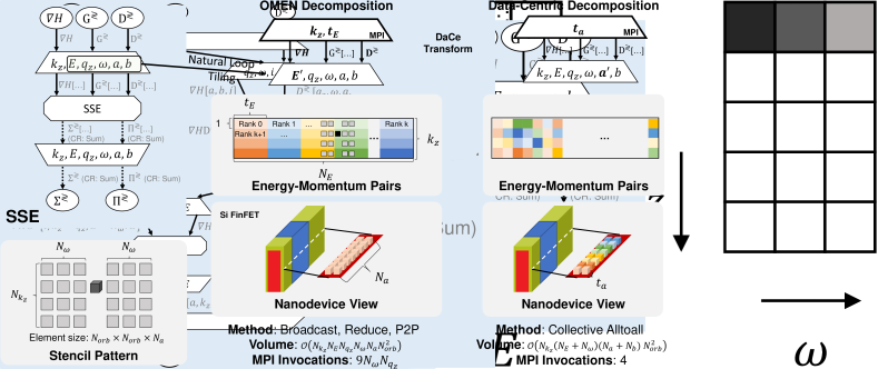
Figure 6. Domain decomposition of SSE in OMEN and DaCe.

We propose a paradigm change by rewriting the quantum transport problem as implemented in OMEN from a data-centric perspective. We show that the key to eliminating the scaling bottleneck is in formulating a communication-avoiding algorithm, which is tightly coupled with recovering local and global data dependencies of the application. We start from a reference Python implementation, using Data-Centric (DaCe) Parallel Programming (Ben-Nun et al., 2019) to express the computations separately from data movement (Fig. 3). DaCe automatically constructs a stateful dataflow view (Fig. 4) that can be used to optimize data movement without modifying the original computation. This enables both rethinking the communication pattern of the simulation, and tuning the data movement for each target supercomputer. In the remainder of this paper, the new code is referred to as DaCe OMEN or simply DaCe.

We report the following innovations, most of them being directly obtained as a result of the data-centric view:

• Data Ingestion: We stage the material and use chunked broadcast to deliver it to nodes. This reduced Piz Daint start-up time at full-scale from $\sim$30 minutes to under two.

• Load Balancing: Similar to OMEN, we divide work among electrons and phonons unevenly, so as to reduce imbalance.

• Communication Avoidance: We reformulate communication in a non-natural way from a physics perspective, leading to two orders of magnitude reduction in volume.

• Boundary Conditions: We pipeline contour integral calculation on the GPUs, computing concurrently and accumulating resulting matrices using on-GPU reduction.

• Sparsity Utilization: We tune and investigate different data-centric transformations on sparse Hamiltonian blocks in GF, using a combination of sparse and dense matrices.

• Pipelining: The DaCe framework automatically generates copy/compute and compute/compute overlap, resulting in 60 auto-generated CUDA streams.

• Computational Innovations: We reformulate SSE computations using data-centric transformations. Using fission and data layout transformations, we reshape the job into a stencil-like strided-batched GEMM operation, where the DaCe implementation yields up to 4.8$\times$ speedup over cuBLAS.

The full implementation details and transformations are described by Ziogas et al. (Ziogas et al., 2019). Below, we highlight the innovations that led to the most significant performance improvements.

5.1. Data-Centric Parallel Programming

Communication-Avoiding (CA) algorithms (Demmel, 2013; Carson et al., 2016) are defined as algorithm variants and schedules (orders of operations) that minimize the total number of performed memory loads and stores, achieving lower bounds in some cases. To achieve such bounds, a subset of those algorithms is matrix-free. A key requirement in modifying an algorithm to achieve communication avoidance is to explicitly formulate its data movement characteristics. The schedule can then be changed by reorganizing the data flow to minimize the sum of accesses in the algorithm. Recovering a data-centric view of an algorithm, which makes movement explicit throughout all levels (from a single core to the entire cluster), is thus the path forward in scaling up the creation of CA variants to more complex algorithms and multi-level memory hierarchies as one.

DaCe defines a development workflow where the original algorithm is independent from its data movement representation, enabling symbolic analysis and transformation of the latter without modifying the scientific code. This way, a CA variant can be formulated and developed by a performance engineer, while the original algorithm retains readability and maintainability. At the core of the DaCe implementation is the Stateful DataFlow multiGraph (SDFG) (Ben-Nun et al., 2019), an intermediate representation that encapsulates data movement and can be generated from high-level code in Python. The syntax (node and edge types) of SDFGs is listed in Fig. 3.

The workflow is as follows: The domain scientist designs an algorithm and implements it with linear algebra operations (imposing dataflow implicitly), or with Memlets and Tasklets (specifying dataflow explicitly). The Memlet edges define all data movement, which is seen in the input and output of each Tasklet, but also entering and leaving Maps with their overall requirements and total number of accesses. This implementation is then parsed into an SDFG, on which performance engineers may apply graph transformations to improve data locality. After transformation, the optimized SDFG is compiled to machine code for performance evaluation. It may be further transformed interactively and tuned for different target platforms and memory hierarchy characteristics. The SDFG representation allows the performance engineer to add local arrays, reshape and nest Maps (e.g., to impose a tiled schedule), fuse scopes, map computations to accelerators (GPUs, FPGAs), and other transformations that may modify the overall number of accesses.

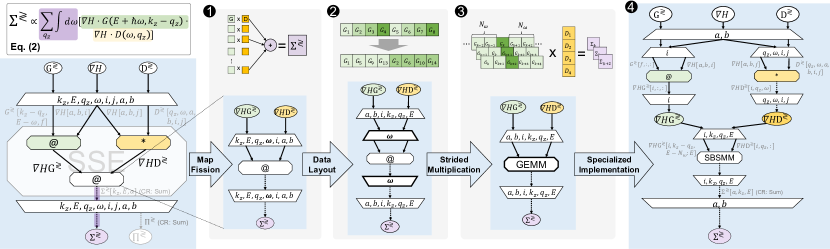
Figure 7. Transforming the dataflow of SSE using SDFGs.

The top-level view of the simulation (Fig. 4) shows that it iterates over two states, GF and SSE. The former computes the boundary conditions, cast them into self-energies, solve for the Green’s Functions, and extract physical observables (current, density) from them. The state consists of two concurrent Maps, one for the electrons and one for the phonons (§ 3.1). The SSE state computes the scattering self-energies ${\mathbf{\Sigma}}^{\gtrless}$ and ${\mathbf{\Pi}}^{\gtrless}$. At this point, we opt to represent the RGF solvers and SSE kernel as Tasklets, i.e., collapsing their dataflow, so as to focus on high-level aspects of the algorithm. This view indicates that the RGF solver cannot compute the Green’s Functions for a specific atom separately from the rest of the material (operating on all atoms for a specific energy-momentum pair), and that SSE outputs the contribution of a specific $\left(k_{z},E,q_{z},\omega,a,b\right)$ point to ${\mathbf{\Sigma}}^{\gtrless}$ and ${\mathbf{\Pi}}^{\gtrless}$. These contributions are then accumulated to the output tensors, as indicated by the dotted Memlet edges. The accumulation is considered associative; therefore the map can compute all dimensions of the inputs and outputs in parallel.

Below we show how the data-centric view is used to identify and implement a tensor-free CA variant of OMEN, achieving near optimal communication for the first time in this scientific domain.

5.2. Communication Avoidance

Figure  6 describes the domain decomposition of SSE computation in OMEN and the DaCe variant, while relevant parameters are given in Table 6. The main part of the computation uses a complex stencil pattern (bottom left of figure) to update 3-D tensors (black cube). In the 2-D stencil, neighboring tensors (grey boxes) are multiplied and accumulated over one full dimension ($N_{k_{z}}$) and one with a radius of $N_{\omega}$ tensors on each side. The domain scientists who first implemented OMEN naturally decomposed the 6D loop nest along the first two dimensions into a $k_{z}\times E/t_{E}$ process grid of energy-momentum pairs (middle part of the figure). In the data-centric view, this original decomposition is expressed as a tiling transformation of the SDFG, where the outermost (top) map controls process mapping. Through sophisticated use of MPI communicators (grouped by rank brightness in the figure) and collectives, OMEN can use broadcast and reduction operations to distribute the data across nodes.

Upon inspecting data movement in the SDFG Memlets, this decomposition yields full data dependencies (Fig. 6, top) and a multiplicative expression for the number of accesses (bottom of figure). If the map is, however, tiled by the atom positions on the nano-device instead (which Eq. (4) does not expose, as it computes one pair), much of the movement can be reduced, as indicated in Fig. 6.

The resulting pair decomposition is rather complex, which would traditionally take an entire code-base rewrite to support, but in our case uses only two graph transformations on the SDFG. We make the modification shown in the top-right of Fig. 6, which leads to an asymptotic reduction in communication volume, speedup of two orders of magnitude, and a reduction in MPI calls to a constant number as a byproduct of the movement scheme (§ 6.1, 7).

5.3. Dataflow Optimizations

The data-centric view not only encompasses macro dataflow that imposes communication, but also data movement within compute devices. We use DaCe to transform all computations in the communication-avoiding variant of OMEN, including the RGF algorithm, SSE, and boundary conditions, and automatically generate GPU code. In Fig. 7 we showcase a subset of these transformations, focusing on a bottleneck subgraph of the simulator, which is found within the SSE kernel: computing ${\mathbf{\Sigma}}^{\gtrless}$ as in Eq. (4). We note that computation of ${\mathbf{\Pi}}^{\gtrless}$ is transformed in a similar manner.

An initial SDFG representation of the ${\mathbf{\Sigma}}^{\gtrless}$ computation is shown on the left side of the figure. In step ❶, we apply Map Fission and isolate the individual operations to separate Maps. This allows storing intermediate results to transient arrays so that they can be reused, effectively lowering the number of multiplications (akin to regrouping algebraic computations in the formula). We then transform each resulting map separately, but focus here on ${\mathbf{\Sigma}}^{\gtrless}$, which results from the accumulation of numerous products of $N_{orb}^{2}$-sized matrices. Since $N_{orb}$ is small (typically ranging between 10 and 25), these multiplications are inefficient and must be transformed.

In step ❷, we reorder the ${\mathbf{\Sigma}}^{\gtrless}$ map dimensions and apply data-layout transformations on the input, transient and output arrays. The new data layout enables representing the $\omega$ map as the innermost dimension and split it out, exposing linear-algebra optimizations. In step ❸, the individual multiplications are aggregated to more efficient GEMM operations using the structure of the map. Furthermore, due to the data re-layout, the inputs and outputs among the sequential GEMM operations are accessed with constant stride. This in turn allows us to use optimized strided-batched operations, such as cublasZgemmStridedBatched from the cuBLAS library. Finally, we specialize the strided-batched operation in DaCe, the performance of which is discussed in § 7.1.5.

In step ❹, the separate maps are fused back together. The optimized SDFG representation of the ${\mathbf{\Sigma}}^{\gtrless}$ computation is depicted on the right-hand side SDFG. All the transformations described above result in an optimized SSE kernel that both reduces the flop count (§ 6.1.1) and has increased computational efficiency (§ 7.1.7).

5.4. Mixed-Precision Computation

The iterative GF-SSE solver creates an opportunity to trade accuracy for performance. The computation of $D^{\gtrless}$ and $G^{\gtrless}$ in the RGF phase consists of deep data dependency graph, whose precision cannot be reduced without substantially impacting the result (Luisier et al., 2011). However, the computation of $\Sigma^{\gtrless}$ in SSE, which is a sum of matrix multiplications, can benefit from half-precision and Tensor Cores.

We adapt the computation in Fig. 7 to use NVIDIA GPU Tensor Cores by transforming the tensors to split-complex format (contiguous real followed by imaginary values), padding the internal matrices to the required 16$\times$16. For normalization, we observe that the dynamic range of the inputs for the multiplications depends on $\nabla H,D^{\gtrless},G^{\gtrless}$, and compute factors based on their magnitudes. Algebraically, denormalization entails scaling by inverse factors. Out-of-range values are clamped to avoid under/overflow and minimize the difference over accumulation, done in double-precision.

6. How Performance Was Measured

To measure the performance of DaCe OMEN and compare it to the state of the art (original code of OMEN), two Si FinFET-like structures similar to the one shown in Fig. 1 have been defined:

• The first one labelled “Small” is characterized by $W=$ 2.1nm and $L=$ 35nm. It exhibits the following parameters: $N_{a}=4{,}864,N_{b}=34,N_{E}=706$, $N_{\omega}=70$, and $N_{k_{z}}$/$N_{qz}$ varying between 3 and 11. Unrealistically small $N_{E}$ and $N_{k_{z}}$/$N_{q_{z}}$ have been chosen to allow the original version of OMEN to simulate it too, but the physical accuracy is not ensured.

• The second one labelled “Large” relies on realistic dimensions ($W=$ 4.8nm and $L=$ 35nm) and physical parameters: $N_{a}=10{,}240,N_{b}=34,N_{E}=1{,}220$, $N_{\omega}=70$, and $N_{k_{z}}$/$N_{qz}$ varying from 5 to 21 to cover both weak and strong scaling.

6.1. Performance Model

The majority of computations revolves around three kernels (§5.1): (a) computation of the boundary conditions; (b) Recursive Green’s Function (RGF); and (c) the SSE kernel. The first two kernels represent most of the computational load of the GF phase, while the SSE phase comprises the SSE kernel. Table 2 shows the flop values, defined empirically and analytically, for the “Small” Silicon structure with varying $N_{k_{z}}$ values.

6.1.1. Computation Model

The kernels of the GF phase mainly involve matrix multiplications between both dense and sparse matrices. The computational complexity of the RGF algorithm for each $\left(k_{z},E\right)$ point is $8\cdot\left(26\cdot bnum-25\right)\left(\frac{N_{a}N_{orb}}{bnum}\right)^{3}+\mathcal{O}\left(\left(\frac{N_{a}N_{orb}}{bnum}\right)^{3}\right)$,
where $bnum$ is the number of diagonal Hamiltonian blocks. The first term accounts for the dense operations, which comprise 90% of the flop count. The latter term is an upper bound on the computational load of the sparse operations. Since the RGF kernel is executed on the GPU, we measure the exact GPU flop count with the NVIDIA profiler nvprof.

In the SSE phase, the flop count of each dense small matrix multiplication (sized $N_{orb}\times N_{orb}$) is $8N_{orb}^{3}$. Thus, the overall flop count for OMEN SSE is $64N_{a}N_{b}N_{3D}N_{k_{z}}N_{q_{z}}N_{E}N_{\omega}N_{orb}^{3}$. The multiplication reduction (algebraic regrouping) powered by the data-centric view (§ 5.3) decreases it by $\frac{2N_{q_{z}}N_{\omega}}{N_{q_{z}}N_{\omega}+1}$, essentially half of the flops for practical sizes.

Table 2. Single Iteration Computational Load^∗ (in Pflop)

	$\boldsymbol{N_{k_{z}}}$
Kernel	3	5	7	9	11
Boundary Conditions	8.45	14.12	19.77	25.42	31.06
RGF	52.95	88.25	123.55	158.85	194.15
SSE (OMEN)	24.41	67.80	132.89	219.67	328.15
SSE (DaCe)	12.38	34.19	66.85	110.36	164.71

^∗: “Small” structure.

6.1.2. Communication Model

Computing ${\mathbf{\Sigma}}^{\gtrless}\left(k_{z},E\right)$ in SSE req-uires each electron pair to execute the following $N_{q_{z}}N_{\omega}$ times:

• Receive the phonon Green’s Functions ${\mathbf{D}}^{\gtrless}(q_{z},\omega)$;

• Receive the electron Green’s Functions ${\mathbf{G}}^{\gtrless}(k_{z}-q_{z},E\pm\omega)$. Symmetrically, send its own electron data ${\mathbf{G}}^{\gtrless}(k_{z},E)$ to the $\left(k_{z}+q_{z},E\mp\omega\right)$ points;

• Accumulate a partial sum of the interactions of the atoms with its neighbors, as described by Eq. (4).

We note that the computation of ${\mathbf{\Pi}}^{\gtrless}$ follows a similar pattern. Putting it all together, the communication scheme for SSE in OMEN is split into $N_{q_{z}}N_{\omega}$ rounds. In each round:

• The phonon Green’s Functions ${\mathbf{D}}^{\gtrless}(\omega,q_{z})$ are broadcast to all electron processes;

• Each electron process iterates over its assigned electron Green’s Functions ${\mathbf{G}}^{\gtrless}(E,k_{z})$ and receives the corresponding ${\mathbf{G}}^{\gtrless}(E\pm\hbar\omega,k_{z}-q_{z})$. In a symmetrical manner, it sends its assigned Green’s Functions to all $\left(k_{z}+q_{z},E\mp\omega\right)$ points;

• The partial phonon self-energies $\Pi_{p}^{\gtrless}(\omega,q_{z})$ produced by each electron process are reduced to ${\mathbf{\Pi}}^{\gtrless}(\omega,q_{z})$ and sent to the corresponding phonon process.

Based on the above, we make the following observations:

• All ${\mathbf{D}}^{\gtrless}$ are broadcast to all electron processes;

• All ${\mathbf{G}}^{\gtrless}$ are replicated through point-to-point communication $2N_{q_{z}}N_{\omega}$ times.

To put this into perspective, consider a “Large” structure simulation with $N_{E}=$ 1,000. The communication aspect of the SSE phase involves each electron process receiving and sending 276 GiB for ${\mathbf{D}}^{\gtrless}$ (${\mathbf{\Pi}}^{\gtrless}$), as well as 2.58 PiB for ${\mathbf{G}}^{\gtrless}$, independent of the number of processes.

In the transformed scheme (Fig. 6, right), each process is assigned a subset of $\frac{N_{a}}{T_{a}}$ atoms and $\frac{N_{E}}{T_{E}}$ electron energies, where $P=T_{a}T_{E}$ is the number of processes. The computations described in Eqs. (4)–(5) require all neighbors per atom, which may or may not be in the same subset. Therefore, the actual number of atoms that each process receives is $\frac{N_{a}}{T_{a}}+c$, where $c$ is the number of neighboring atoms that are not part of the subset. We over-approximate $c$ by $N_{b}$. In a similar manner, each process is assigned $\frac{N_{E}}{T_{E}}+2N_{\omega}$ energies.

We implement the distribution change with all-to-all collective operations (MPI_Alltoallv in the MPI standard). We use four collectives on ${\mathbf{G}}^{\gtrless}$, ${\mathbf{D}}^{\gtrless}$, ${\mathbf{\Sigma}}^{\gtrless}$, and ${\mathbf{\Pi}}^{\gtrless}$, where each process contributes:

• $64N_{k_{z}}\left(\frac{N_{E}}{T_{E}}+2N_{\omega}\right)\left(\frac{N_{a}}{T_{a}}+N_{b}\right)N_{orb}^{2}$ bytes for ${\mathbf{G}}^{\gtrless}$ and ${\mathbf{\Sigma}}^{\gtrless}$;

• $64N_{q_{z}}N_{\omega}\left(\frac{N_{a}}{T_{a}}+N_{b}\right)(N_{b}+1)N_{3D}^{2}$ bytes for ${\mathbf{D}}^{\gtrless}$ and ${\mathbf{\Pi}}^{\gtrless}$.

We quantify the communication volumes for a typical problem size in Tables 3 and 4, the former with varying $N_{k_{z}}$ and the latter with fixed parameters. Both tables highlight a clear advantage in favor of the communication-avoiding variant, communicating two orders less than the state of the art. For the large-scale simulation described above, the new communication approach (with $T_{a}=P,T_{E}=1$) distributes the 276 GiB for ${\mathbf{D}}^{\gtrless}$ and ${\mathbf{\Pi}}^{\gtrless}$ over all processes, and only adds a minor overhead of 28.26 MiB per process. It also lowers the fixed cost of 2.58 PiB for ${\mathbf{G}}^{\gtrless}$ and ${\mathbf{\Sigma}}^{\gtrless}$ to only 1.8 TiB distributed to all processes and 6.13 GiB per process. We note that the total cost for ${\mathbf{G}}^{\gtrless}$ becomes equal for the two communication schemes when the number of processes is greater than 440,000.

Table 3. SSE Communication Volume^∗ Weak Scaling (TiB)

	$\boldsymbol{N_{k_{z}}}$ (Processes)
Variant	3 (768)	5 (1280)	7 (1792)	9 (2304)	11 (2816)
OMEN	32.11	89.18	174.80	288.95	431.65
DaCe	0.54 [59$\times$]	1.22 [73$\times$]	2.17 [81$\times$]	3.38 [85$\times$]	4.86 [89$\times$]

^∗: “Small” structure, reduction ratio in brackets.

Table 4. SSE Communication Volume^∗ Strong Scaling (TiB)

	Processes
Variant	224	448	896	1792	2688
OMEN	108.24	117.75	136.76	174.80	212.84
DaCe	0.95 [114$\times$]	1.13 [104$\times$]	1.48 [92$\times$]	2.17 [80$\times$]	2.87 [74$\times$]

^∗: “Small” structure, $N_{k_{z}}=7$, reduction ratio in brackets.

6.2. Selected HPC Platforms

The two systems we run DaCe OMEN experiments on are CSCS Piz Daint (Centre, 2019) (6th place in June 2019’s Top500 supercomputer list (TOP500.org, 2019)) and OLCF Summit (Facility, 2019) (1st place). Piz Daint is composed of 5,704 Cray XC50 compute nodes, each equipped with a 12-core HT-enabled (2-way SMT) Intel Xeon E5-2690 v3 CPU with 64 GiB RAM (peaking at 499.2 double-precision Gflop/s), and one NVIDIA Tesla P100 GPU (4.7 Tflop/s). The nodes communicate using Cray’s Aries interconnect. Summit comprises 4,608 nodes, each containing two IBM POWER9 CPUs (21 usable physical cores with 4-way SMT, 515.76 Gflop/s) with 512 GiB RAM and six NVIDIA Tesla V100 GPUs (42 double-precision Tflop/s in total, 720 half-precision Tflop/s using Tensor Cores). The nodes are connected using Mellanox EDR 100G InfiniBand organized in a Fat Tree topology. For Piz Daint, we run our experiments with two processes per node (sharing the GPU), apart from a full-scale run on 5,400 nodes, where the simulation parameters do not produce enough workload for more than one process per node. In Summit we run with six processes per node, each consuming 7 physical cores. We conduct experiments at least 5 times, reporting the median and 95% Confidence Interval.

Despite the fact that both systems feature GPUs as their main workhorse, the rest of the architecture is quite different. While Piz Daint has a reasonable balance between CPU and GPU performance (GPU/CPU ratio of 9.4$\times$), Summit’s POWER9 CPUs are significantly (81.43$\times$) weaker than the six V100 GPUs present on each node. Tuning our data-centric simulator, which utilizes both the CPU and GPUs, we take this into account by assigning each architecture different tile sizes and processes per node, so as to balance the load without running out of memory.

7. Performance Results

We proceed to evaluate the performance of the data-centric OMEN algorithm. Starting with per-component benchmarks, we demonstrate the necessity of specialized implementations, and that critical portions of the algorithm are sufficiently tuned to the underlying systems. We then measure performance aspects of OMEN and the DaCe variant on the “Small” problem, consisting of 4,864 atoms, on up to 5,400 Piz Daint and 1,452 Summit GPUs. Lastly, we measure the heat dissipation of the “Large”, 10,240 atom nanodevice on up to 27,360 Summit GPUs.

7.1. Component Benchmarks

Below we present individual portions of the quantum transport simulation pipeline, including data I/O, overlapping, computational aspects of GF, SSE, and total single node performance.

7.1.1. Data Ingestion

The input of the simulator is material and structural information of the nano-device in question (produced by CP2K). The size of this data typically ranges between the order of GiBs to 10s of GiBs, scattered across multiple files. Once the data is loaded and pre-processed for each rank, the OMEN algorithm does not require additional I/O, and can operate with the information dispersed across the processes. Despite being a constant overhead, without proper data staging, running at large scale quickly becomes infeasible due to contention on the parallel filesystem. For example, running on Piz Daint at near-full scale (5,300 nodes) takes over 30 minutes of loading, and with 2,589 nodes takes 1,112 seconds.

To reduce this time, we stage the nanostructure information and broadcast relevant information in chunks to the participating ranks. As expected, this reduces start-up time to under a minute in most cases, and 31.1 seconds for 4,560 nodes. As the solver normally takes 20–100 iterations to converge, we also report time-per-iteration factoring for I/O overhead w.r.t. 50 iterations.

7.1.2. Recomputation Avoidance

For each iteration of the Green’s Function phase and for each energy-momentum point, three operations are performed: (a) specialization of the input data, (b) computation of the boundary conditions, and (c) execution of the RGF kernel. From a data-centric perspective, the first two operations induce data dependencies on specific energy-momentum points, but not on the iteration. Therefore, it is possible to perform them once during an initialization phase and reuse the produced output in all iterations. However, the memory footprint to avoid recomputation is immense: specialization data for the “Large” nanodevice consumes 3GB per-point, while the boundary conditions need another 1GB. We leverage the compute-memory tradeoff by enabling three modes of executing the GF phase: (a) “No Cache”: data is recomputed in every iteration; (b) “Cache Boundary Conditions”, where data is only re-specialized per-iteration; and (c) “Cache BC+Spec.”: both specialized data and boundary conditions are cached in memory.

7.1.3. Automatic Pipelining

Since parallelism is expressed natively in SDFGs, the DaCe framework schedules independent nodes concurrently, using threads for CPU and CUDA streams for GPU. DaCe automatically generates 32 and 60 streams for electron and phonon GF computations, respectively. We vary the maximum number of concurrent streams on a single electron point on Summit and report the results in Table 5. The results imply that more than 16 streams are necessary to yield the 7.5% speedup in the table, automatically achieved as a byproduct of data-centric parallel programming.

Table 5. CUDA Streams in Green’s Functions (Summit)

Streams	1	2	4	16	Auto (32)
Time [s]	10.07	9.94	9.86	9.61	9.32 (2.63 Tflop/s)

7.1.4. Green’s Functions and Sparsity

Since the RGF algorithm uses a combination of sparse and dense matrices, several alternatives exist to perform the required multiplications. In particular, a common operation in RGF is F[n] @ gR[n + 1] @ E[n + 1] — multiplying two blocks ($E$, $F$) of the block tri-diagonal Hamiltonian matrix ($H$) with a retarded Green’s Functions block ($gR$). The off-diagonal blocks are typically sparse CSR matrices, but can also be stored in CSC format if needed. To perform this operation, one can either use CSR-to-dense conversion followed by dense multiplication (GEMM); or use sparse-dense multiplications (CSRMM). These options can be interchanged via data-centric transformations.

Table 6. Matrix Multiplication Performance

		Operation
GPU	Method	NN	NT	TN	TT
P100	GEMM	100.337 ms	99.306 ms	101.959 ms	100.857 ms
	CSRMM2	15.937 ms	11.437 ms	85.573 ms	—
	GEMMI	30.861 ms	—	—	—
V100	GEMM	58.382 ms	58.144 ms	58.666 ms	58.315 ms
	CSRMM2	8.202 ms	6.14 ms	52.722 ms	—
	GEMMI	15.198 ms	—	—	—

In Table 6 we study the performance of the different methods in cuBLAS and cuSPARSE, on the P100 and V100 GPUs. The CSRMM2 method multiplies a CSR matrix (on the left side) with a dense matrix and supports NN, NT, and TN operations. The GEMMI method multiplies a dense matrix with a CSC matrix (on the right side) and only supports NN. In Table 7 we study the performance of three different approaches to compute the above product. In the first approach, we use dense multiplication twice. In the second approach, we assume that both $F$ and $E$ are CSR matrices. We first compute the product of $E$ and $gR$ with CSRMM2 in TN operation. Subsequently, we multiply the intermediate result with $F$ using GEMMI. In the third approach, $F$ is in CSR format while $E$ is given in CSC. We compute the product of $F$ and $gR$ with CSRMM2 in NT operation. Using a second identical operation we multiply $E$ with the intermediate result. We observe that the best performance is attained with the third approach, with 5.10–9.74$\times$ speedup over other GPU implementations.

Table 7. 3-Matrix Multiplication Performance

	Approach
GPU	GEMM/GEMM	CSRMM2/GEMMI	CSRMM2/CSRMM2
P100	200.879 ms	116.380 ms	22.798 ms
V100	116.881 ms	67.924 ms	11.994 ms

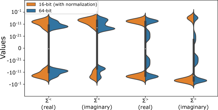
(a) Output Distribution (Non-Zero Values)

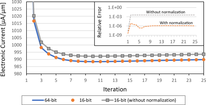
(b) Convergence

Figure 8. Comparison of double- and half-precision SSE.

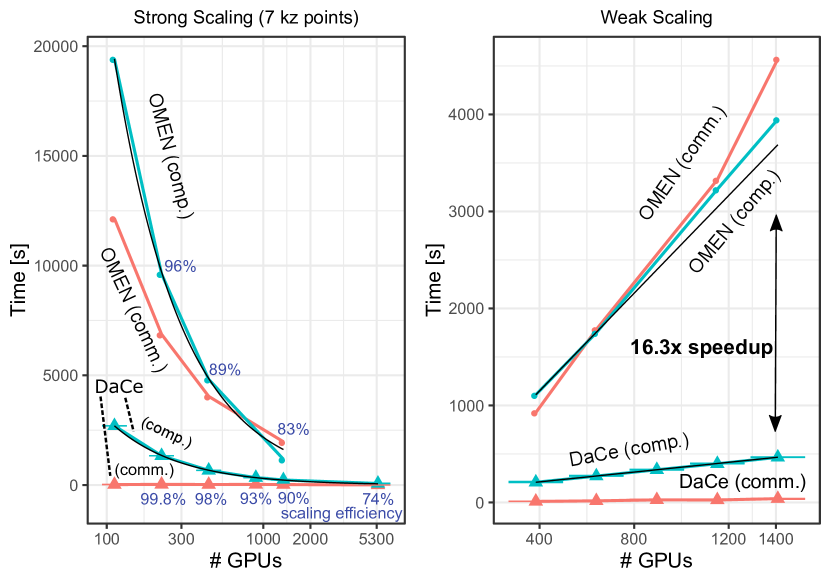
(a) Piz Daint

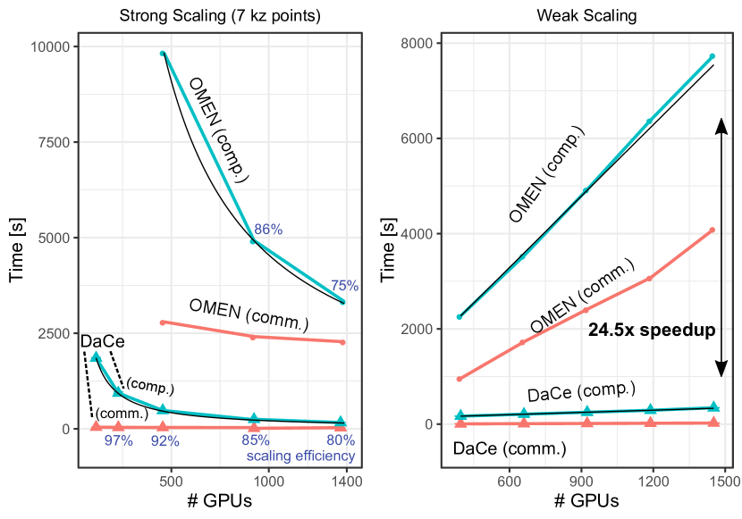
(b) Summit

Figure 9. DaCe OMEN simulation scalability ($N_{a}=4{,}864$, black lines: ideal scaling).

7.1.5. Custom Strided Multiplication

As part of SSE dataflow transformations (§ 5.3), we reformulate a multitude of small-scale matrix multiplications into one “strided and batched” GEMM operation (Fig. 7, step ❸). We thus initially opt to use the highly-tuned NVIDIA cuBLAS library for the computation, which yields 85.7% of peak double-precision flop/s on average. However, upon deeper inspection using the performance model (§ 6.1.1), we observe a discrepancy, where the useful operations/second with respect to the actual sizes is only around 6% of the GPU peak performance. As our individual matrices are small (typically 12$\times$12), this effect may stem from excessive padding in cuBLAS, which is tuned specifically for common problem sizes.

Table 8. Strided Matrix Multiplication Performance

	cuBLAS			DaCe (SBSMM)
GPU	Gflop	Time	% Peak (Useful)	Gflop	Time	% Peak
P100	27.42	6.73 ms	86.6% (6.1%)	1.92	4.03 ms	10.1%
V100	27.42	4.62 ms	84.8% (5.9%)	1.92	0.70 ms	39.1%
V100-TC	—	—	—	3.42	0.13 ms	—

We use DaCe to create two specialized strided-batched small-scale matrix multiplication tasklets (SBSMM in Fig. 7), and report their performance in Table 8. The double-precision tasklet maximizes parallelism based on the problem size and does not pad data; whereas the half-precision tasklet utilizes Tensor Cores (§5.4) for complex matrix multiplications. As shown in the table, SBSMM is 5.76$\times$ (64-bit) to 31$\times$ (16-bit) faster than cuBLAS, which does not support half-complex multiplication, demonstrating that performance engineers can use the data-centric view to partition specific problems in ways not considered by vendor HPC libraries.

7.1.6. Mixed-Precision Convergence

Figures 8(a) and 8(b) depict the output value distribution and convergence of the electronic current for SSE and the reduced-precision scheme (SSE-16, § 5.4) for the “Large” structure. When normalization is applied, SSE-16 produces similar outputs per step and converges at the same rate as SSE, to a value that relatively differs by $1.2\cdot 10^{-6}$. In comparison, without scaling $D^{\gtrless},G^{\gtrless}$, the relative error increases to 0.003. The core multiplication kernels, SBSMM, yield 14.78 Tflop/s per-GPU, 404.41 Pflop/s in total over 4,560 Summit nodes.

7.1.7. Single-Node Performance

We evaluate the performance of OMEN, the DaCe variant, and the Python implementation (using the numpy module implemented over MKL), on the “Small” Silicon nanostructure with $N_{k_{z}}=3$. Table 9 shows the runtime of the GF and SSE SDFG states, for $\frac{1}{384}$ of the total computational load, executed by a single node on Piz Daint. Although Python uses optimized routines, it exhibits very slow performance on its own. This is a direct result of utilizing an interpreter for mathematical expressions, where arrays are allocated at runtime and each operation incurs high overheads. This can especially be seen in SSE, which consists of many small multiplication operations. The table also indicates that the data-centric transformations made on the Python code using DaCe outperforms the manually-tuned C++ OMEN on both phases, where the performance-oriented reconstruction of SSE generates a speedup of 9.97$\times$.

Table 9. Piz Daint Single-Node Performance

	Phase
Variant	GF			SSE
	Tflop	Time [s]	% Peak	Tflop	Time [s]	% Peak
OMEN	174.0	144.14	23.2%	63.6	965.45	1.3%
Python	174.0	1,342.77	2.5%	63.6	30,560.13	0.2%
DaCe	174.0	111.25	30.1%	31.8	29.93	20.4%

7.1.8. Communication

We study DaCe OMEN’s communication efficiency on the Summit supercomputer. We utilize MPI_Alltoallv to exchange $D^{\gtrless}$, $\Pi^{\gtrless}$, $G^{\gtrless}$, and $\Sigma^{\gtrless}$. In this collective call, each rank sends a different amount of data to all other ranks, performed in several rounds (Prisacari et al., 2013). For OMEN, the communication pattern is sparse for some of the calls. We derive lower bounds for the completion time of each call by counting the amount of data each node must send (aggregating over all ranks on the same node), and dividing that by the injection bandwidth of a Summit node of 23 GB/s (Facility, 2019).

For the large-scale run, our model predicts 1.85s of runtime to communicate each of $D^{\gtrless}$/$\Pi^{\gtrless}$ and 0.21s to communicate each of $G^{\gtrless}$/$\Sigma^{\gtrless}$ at 100% of injection bandwidth utilization. Our measurements (§ 7.3) show that we achieve 84.57% and 42.32% of that (2.18s and 0.55s actual runtime for $D^{\gtrless}$/$\Pi^{\gtrless}$ and $G^{\gtrless}$/$\Sigma^{\gtrless}$, respectively).

7.2. Scalability

The communication-avoiding variant of OMEN (DaCe OMEN) scales well to the full size of both supercomputers. In Fig. 9, we measure the runtime and scalability of a single GF-SSE iteration of OMEN and the DaCe variant on Piz Daint and Summit. For strong scaling, we use the “Small” structure and fix $N_{k_{z}}=7$ (so that OMEN can treat it), running with 112–5,400 nodes on Piz Daint and 19–228 nodes (114–1,368 GPUs) on Summit. For weak scaling, we annotate ideal scaling (in black) with proportional increases in the number of $k_{z}$ points and nodes, since the GF and SSE phases scale differently relative to the simulation parameters, by $N_{k_{z}}$ and $N_{k_{z}}N_{q_{z}}=N_{k_{z}}^{2}$, respectively. We measure the same structure with varying $k_{z}$ points: $N_{k_{z}}\in\left\{3,5,7,9,11\right\}$, using 384–1,408 nodes on Piz Daint and 66–242 nodes (396–1,452 GPUs) on Summit.

Compared with the original OMEN, the DaCe variant is efficient, both from the computation and communication aspects. On Piz Daint, the total runtime of the reduced-communication variant outperforms OMEN, the current state of the art, up to a factor of 16.3$\times$, while the communication time improves by up to 417.2$\times$. On Summit, the total runtime improves by up to factor of 24.5$\times$, while communication is sped up by up to 79.7$\times$. Moreover, the higher the simulation accuracy ($N_{k_{z}}$), the greater the speedup is.

The speedup of the computational runtime on Summit is higher than on Piz Daint. This is the result of OMEN depending on multiple external libraries, some of which are not necessarily optimized for every architecture (e.g., IBM POWER9). On the other hand, SDFGs are compiled on the target architecture and depend only on a few optimized libraries provided by the architecture vendor (e.g., MKL, cuBLAS, ESSL), whose implementations can always be replaced by SDFGs for further tuning and transformations.

As for scaling efficiency, on Summit DaCe OMEN achieves a speedup of 9.68$\times$ on 12 times the nodes in the strong scaling experiment (11.23$\times$ for computation alone). Piz Daint yields similar results with 10.69$\times$ speedup. The algorithm weakly scales with $N_{k_{z}}$ on both platforms, again an order of magnitude faster than the state of the art on structures of the same size. We thus conclude that the data-centric variant of OMEN is strictly desirable over the original.

7.3. Extreme-Scale Runs

We run DaCe OMEN on a setup not possible on the original OMEN, due to infeasible memory requirements. We simulate the “Large” 10,240 atom nanostructure — a size never-before-simulated with GF+SSE at the ab initio level — using the DaCe variant of OMEN. For this purpose, we use up to 98.96% of the Summit supercomputer, 27,360 GPUs, and run our proposed Python code with 21 $k_{z}$ points, which are necessary to produce accurate results (see Table 6).

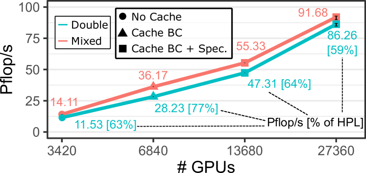
Figure 10. Strong scaling on Summit, “Large” structure.

Figure 10 plots the results of the strong-scaling experiment, using 3,420 GPUs for the baseline. The simulation costs 8.17–9.41 Exaflop per iteration, depending on the caching strategy (specialization and/or boundary conditions, § 7.1.2). Sustained performance of 85.45 Pflop/s (42.55% of supercomputer peak) is achieved in double precision, and 90.89.68 Pflop/s in mixed precision, including communication, I/O, and caching as described above. A full breakdown is listed in Table 10. The table compares performance with machine peak and effective maximum performance (HPL, 148.6 Pflop/s for Summit (TOP500.org, 2019)). Additionally, we compare the per-atom performance of the DaCe variant with the original OMEN on 6,840 Summit GPUs. Both implementations execute a simulation with 21 $k_{z}$ points and 1,220 electron energies, but different number of atoms. As shown in Table 11, DaCe OMEN is up to two orders of magnitude faster per-atom. These results prove that the electro-thermal properties of nano-devices of this magnitude can be computed in under 2 minutes per iteration, as desired for practical applications.

Table 10. Full-Scale 10,240 Atom Run Breakdown

Phase	Time	Eflop	Pflop/s	% Max	% Peak
Data Ingestion	31.10	—	—	—	—
Boundary Conditions	30.51	1.23	40.40	27.19%	20.12%
GF	41.36	6.00	145.01	97.59%	72.22%
SSE (double-precision)	41.91	2.18	51.94	34.95%	25.87%
SSE (mixed-precision)	36.16	2.18	60.21	—	—
Communication	11.50	—	—	—	76.72%
Total	94.77	8.17	86.26	58.05%	42.96%
Total (incl. I/O and Init.)	96.00	8.20	85.45	57.50%	42.55%
Total (mixed-precision)	89.02	8.17	91.68	—	—
Total (incl. I/O and Init.)	90.25	8.20	90.89	—	—

Table 11. Per-Atom Performance

Variant	$N_{a}$	Time [s]	Time/Atom [s]	Speedup
OMEN	1,064	4,695.70	4.413	1.0x
DaCe	10,240	333.36	0.033	140.9x

$P=6{,}840,N_{b}=34,N_{orb}=12,N_{E}=1{,}220,N_{\omega}=70$.

To gain insight on the factors that limit the performance of DaCe OMEN, we analyze the bottlenecks of each phase in Table 10. We use the Roofline model (Williams et al., 2009) to depict the limits of the main phases in Fig. 11. The GF phase, as seen in Fig. 11, is compute-bound, achieving 97.59% of HPL performance. In contrast, the SSE phase combines a multitude of small matrix multiplications, which were shown to be memory-bound (Masliah et al., 2016). This agrees with our empirical results, in which the memory per batched multiplication is small enough to fit in the L2 cache, and operational intensity is too low to be compute-bound. Mixed-precision SSE (Fig. 11, SSE-16) improves I/O by reducing element size, but is still limited by memory bandwidth from a data-centric perspective. Communication (§ 7.1.8 for a full model) is a sparse alltoall collective, which achieves in total 76.72% bandwidth utilization and cannot be overlapped with computation algorithmically.

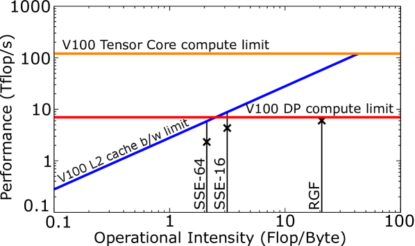
Figure 11. Roofline model of the computational kernels.

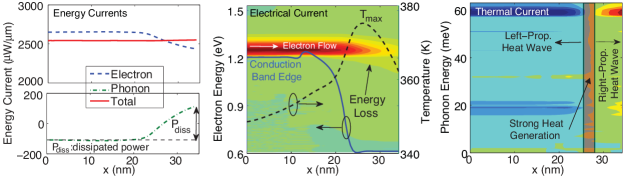
Figure 12. Electro-thermal simulation of a FinFET with $W$=2.1nm and $L$=35nm (“Small” structure from Section 6, same as in Fig. 1). The energy (left), electrical (middle), and thermal (right) currents are shown at $V_{gs}$=0.5 V and $V_{ds}$=0.6 V.

8. Implications

8.1. Quantum Transport Simulations

With DaCe OMEN, the electro-thermal properties of FinFET-like structures can now be simulated within ultra-short times. An example is shown in Fig. 12. The left sub-plot represents the electron (dashed blue line) and phonon (dashed-dotted green line) energy currents that flow through the considered device. As their sum is constant over the entire FinFET axis $x$ (solid red line), it can be inferred that energy is conserved and that the GF+SSE model was correctly implemented. The following information can be extracted from the data: (i) dissipated power (left plot), (ii) spectral distribution of the electrical current (middle plot, red indicates high current concentrations, green none), (iii) average crystal temperature along the $x$-axis (middle plot), and (iv) heat propagation map (right plot, red: heat flow towards left, blue: heat flow towards right). The atomically resolved temperature of this system was already presented in Fig. 1(d). It turns out that most of the heat is generated close to the end of the transistor channel ($x$=27nm). From there, it propagates towards the source ($x$=0) and drain ($x$=$L$) extensions, where it is absorbed by the metal contacts. It can also be seen that the location with the highest heat generation rate coincides with the maximum of the crystal temperature ($T_{max}$). Both are situated in a region with a high electric field, where electrons are prone to emit phonons.

Heat dissipation does not only affect the behavior of nano-scale transistors, but also of a wide range of other nano-devices. For example, Lithium-ion batteries (LIBs), under unfavorable operating conditions, can overheat and endanger the security of the objects and persons surrounding them. Understanding how heat is created in these energy storage units (chemical reaction, Joule heating, other) and providing design guidelines to reduce the temperature of their active region are two objectives of utmost importance. Other nano-structures such as non-volatile phase change random access memories (PCRAM) leverage Joule heating to undergo a transition from an amorphous to a crystalline phase. By better controlling this electro-thermal phenomenon, it will be possible to obtain a more gradual change from their high- to their low-resistance state such that PCRAMs can act as solid-state synapses in “non von Neumann” neuromorphic computing circuits. Current research in nano-transistors, LIBs, and PCRAM cells, to cite a few applications, is expected to benefit from the improvements that have been made to the electro-thermal model of OMEN. Structure dimensions that were believed to belong to the world of the imaginary are now accessible within short turn-around times. Consequently, the proposed code will allow to establish new bridges with experimental groups working on nano-devices subject to strong heating effects.

8.2. Data-Centric Parallel Programming

The paper demonstrates how modifications to data movement alone can transform a complex, nonlinear solver to become communication efficient. Through modeling made possible by a data-centric intermediate representation, and graph transformations of the underlying macro- and micro- dataflow, this work is the first to introduce communication-avoiding principles to a full application.

Because of the underlying retargetable SDFG representation, the solver runs on two different top-6 supercomputers efficiently, relying only on MPI and one external HPC library (BLAS) per-platform. The SDFG was generated from a Python source code five times shorter than OMEN, and itself contains 2,015 nodes after transformations, created without modifying the original operations. The resulting performance is two orders of magnitude faster per-atom than the fine-tuned state of the art, which was recognized twice as a Gordon Bell finalist. This implies that overcoming scaling bottlenecks today requires reformulation and nontrivial decompositions, whose examination is facilitated by the data-centric paradigm.

- (1)
- Ben-Nun et al. (2019) T. Ben-Nun, J. de Fine Licht, A. N. Ziogas, T. Schneider, and T. Hoefler. 2019. Stateful Dataflow Multigraphs: A Data-Centric Model for Performance Portability on Heterogeneous Architectures. In Proc. Int’l Conference for High Performance Computing, Networking, Storage and Analysis.
- Calderara et al. (2015) M. Calderara, S. Brück, A. Pedersen, M. H. Bani-Hashemian, J. VandeVondele, and M. Luisier. 2015. Pushing Back the Limit of Ab-initio Quantum Transport Simulations on Hybrid Supercomputers. In Proc. Int’l Conference for High Performance Computing, Networking, Storage and Analysis (SC ’15). ACM, 3:1–3:12.
- Carson et al. (2016) E. Carson, J. Demmel, L. Grigori, N. Knight, P. Koanantakool, O. Schwartz, and H. V. Simhadri. 2016. Write-Avoiding Algorithms. In 2016 IEEE Int’l Parallel and Distributed Processing Symposium (IPDPS). 648–658.
- Centre (2019) Swiss National Supercomputing Centre. 2019. Piz Daint. https://www.cscs.ch/computers/piz-daint/
- Datta (1995) S. Datta. 1995. Electronic Transport in Mesoscopic Systems. Cambridge Uni. Press.
- Demmel (2013) J. Demmel. 2013. Communication-avoiding algorithms for linear algebra and beyond. In IEEE 27th Int’l Symposium on Parallel and Distributed Processing.
- Facility (2019) Oak Ridge Leadership Computing Facility. 2019. Summit. https://www.olcf.ornl.gov/olcf-resources/compute-systems/summit/
- Ferrer et al. (2014) J. Ferrer, C. J. Lambert, V. M. García-Suárez, D. Manrique, D. Visontai, L. Oroszlany, R. Rodríguez-Ferradás, I. Grace, S. W. D. Bailey, K. Gillemot, et al. 2014. GOLLUM: a next-generation simulation tool for electron, thermal and spin transport. New Journal of Physics 16, 9 (2014), 093029.
- Grenoble (2013) CEA Grenoble. 2013. TB_Sim. http://inac.cea.fr/L_Sim/TB_Sim/
- Groth et al. (2014) C. W. Groth, M. Wimmer, A. R. Akhmerov, and X. Waintal. 2014. Kwant: a software package for quantum transport. New Journal of Physics 16, 6 (2014).
- Group and Klimeck (2018) The Nanoelectronic Modeling Group and Gerhard Klimeck. 2018. NEMO5. https://engineering.purdue.edu/gekcogrp/software-projects/nemo5/
- Kohn and Sham (1965) W. Kohn and L. J. Sham. 1965. Self-Consistent Equations Including Exchange and Correlation Effects. Phys. Rev. 140 (Nov 1965), A1133–A1138. Issue 4A.
- Luisier (2010) M. Luisier. 2010. A Parallel Implementation of Electron-Phonon Scattering in Nanoelectronic Devices up to 95k Cores. In SC ’10: Proc. ACM/IEEE Int’l Conference for High Performance Computing, Networking, Storage and Analysis. 1–11.
- Luisier et al. (2011) M. Luisier, T. B. Boykin, G. Klimeck, and W. Fichtner. 2011. Atomistic Nanoelectronic Device Engineering with Sustained Performances Up to 1.44 PFlop/s. In Proc. Int’l Conference for High Performance Computing, Networking, Storage and Analysis (SC ’11). ACM, 2:1–2:11.
- Luisier et al. (2006) M. Luisier, A. Schenk, W. Fichtner, and G. Klimeck. 2006. Atomistic simulation of nanowires in the tight-binding formalism: From boundary conditions to strain calculations. Phys. Rev. B 74 (2006), 12. Issue 20.
- Masliah et al. (2016) I. Masliah, A. Abdelfattah, A. Haidar, S. Tomov, M. Baboulin, J. Falcou, and J. Dongarra. 2016. High-Performance Matrix-Matrix Multiplications of Very Small Matrices. In Proc. 22Nd Int’l Conference on Euro-Par 2016: Parallel Processing - Volume 9833. Springer-Verlag New York, Inc., 659–671.
- NanoTCAD (2017) NanoTCAD. 2017. ViDES. http://vides.nanotcad.com/vides/
- P. McCormick (2019) P. McCormick. 2019. Yin & Yang: Hardware Heterogeneity & Software Productivity . Talk at SOS23 meeting, Asheville, NC.
- Pawlik (2016) R. Pawlik. 2016. Current CPUs produce 4 times more heat than hot plates. https://cloudandheat.com/blog/current-cpus-produce-4-times-more/
- Pop et al. (2006) E. Pop, S. Sinha, and K. E. Goodson. 2006. Heat Generation and Transport in Nanometer-Scale Transistors. Proc. IEEE 94, 8 (Aug 2006), 1587–1601.
- Prisacari et al. (2013) B. Prisacari, G. Rodriguez, C. Minkenberg, and T. Hoefler. 2013. Bandwidth-optimal all-to-all exchanges in fat tree networks. In Proc. 27th Int’l ACM conference on supercomputing. ACM, 139–148.
- Stieger et al. (2017) C. Stieger, A. Szabo, T. Bunjaku, and M. Luisier. 2017. Ab-initio quantum transport simulation of self-heating in single-layer 2-D materials. Journal of Applied Physics 122, 4 (2017), 045708.
- Svizhenko et al. (2002) A. Svizhenko, M. P. Anantram, T. R. Govindan, B. Biegel, and R. Venugopal. 2002. Two-dimensional quantum mechanical modeling of nanotransistors. Journal of Applied Physics 91, 4 (2002), 2343–2354.
- Synopsys (2019) Synopsys. 2019. QuantumATK. http://synopsys.com/silicon/quantumatk.html
- TOP500.org (2019) TOP500.org. 2019. TOP500 Supercomputer Sites.
- Unat et al. (2017) D. Unat et al. 2017. Trends in Data Locality Abstractions for HPC Systems. IEEE Transactions on Parallel and Distributed Systems 28, 10 (Oct 2017), 3007–3020.
- VandeVondele et al. (2005) J. VandeVondele, M. Krack, F. Mohamed, M. Parrinello, T. Chassaing, and J. Hutter. 2005. Quickstep: Fast and accurate density functional calculations using a mixed Gaussian and plane waves approach. Comput. Phys. Comm. 167, 2 (2005), 103–128.
- Wei (2008) J. Wei. 2008. Challenges in Cooling Design of CPU Packages for High-Performance Servers. Heat Transfer Engineering 29, 2 (2008), 178–187.
- Williams et al. (2009) S. Williams, A. Waterman, and D. Patterson. 2009. Roofline: An Insightful Visual Performance Model for Multicore Architectures. Commun. ACM 52, 4 (2009).
- Ziogas et al. (2019) A. N. Ziogas, T. Ben-Nun, G. Indalecio Fernandez, T. Schneider, M. Luisier, and T. Hoefler. 2019. Optimizing the Data Movement in Quantum Transport Simulations via Data-Centric Parallel Programming. In Proc. Int’l Conference for High Performance Computing, Networking, Storage and Analysis.