Direct determination of cosmic string loop density from simulations

Abstract

We determine the distribution of cosmic string loops directly from simulations, rather than determining the loop production function and inferring the loop distribution from that. For a wide range of loop lengths, the results agree well with a power law exponent $-2.5$ in the radiation era and $-2$ in the matter era, the universal result for any loop production function that does not diverge at small scales. Our results extend those of Ringeval, Sakellariadou, and Bouchet: we are able to run for 15 times longer in conformal time and simulate a volume 300–2400 times larger. At the times they reached, our simulation is in general agreement with the more negative exponents they found, $-2.6$ and $-2.4$. However, our simulations show that this was a transient regime; at later times the exponents decline to the values above. This provides further evidence against models with a rapid divergence of the loop density at small scales, such as “model 3” used to analyze LIGO data and predict LISA sensitivity.

I Introduction

Cosmic strings are long, thin objects which may form by the Kibble mechanism during a symmetry-breaking transition in the early universe Kibble (1976); Vilenkin and Shellard (2000), or they may be the strings of string theory (or one-dimensional D-branes) left over from a string-theory inflationary scenario Dvali and Vilenkin (2004); Copeland et al. (2004). In the simplest scenarios, which we consider here, strings have no ends, but exist in a “network” made up of infinite strings and a distribution of loops of all sizes.

Intercommutation breaks off loops from infinite strings or from larger loops. Over time, energy flows from infinite strings into loops, and is eventually radiated in gravitational waves. (We will consider only the case where there is no other channel through which loops may lose their energy.) This flow of energy prevents strings from coming to dominate the universe as monopoles would. Instead the string network scales, with all linear measures of string properties being proportional to the age of the universe $t$. The infinite string density scales as radiation in radiation era and as matter in the matter era.

Many potentially observable signals of a cosmic string network depend on the loop distribution. In particular, the best way of discovering a cosmic string network is to observe the gravitational waves coming from loops Damour and Vilenkin (2005); Siemens et al. (2006); Sanidas et al. (2012); Binetruy et al. (2012); Sousa and Avelino (2016); Kuroyanagi et al. (2012); Blanco-Pillado and Olum (2017); Abbott et al. (2018); Auclair et al. (2019a). The non-observation of such signals, by pulsar timing experiments, currently provides the strongest bounds on the energy scale of the string network Blanco-Pillado et al. (2018). Thus it is very important to determine the distribution of cosmic string loops.

Two methods have been used to determine the loop distribution. The simplest is just to examine the distribution of loops existing at several times during the simulation. Then exhibit the distribution in scaling units, so that in the scaling regime, it would not change with time. Identify the section of the distribution that seems to be unchanging to find the scaling distribution. This technique was used early on by Albrecht and Turok Albrecht and Turok (1989), and then by Ringeval, Sakellariadou and Bouchet Ringeval et al. (2007), who found that the loop number density scaled as loop length to the power -2.60 in the radiation era and -2.41 in the matter era.

The second technique is to study the rate at which loops of different sizes are produced. By showing this in scaling units, determine the scaling loop production function. Then use cosmological kinematics to go from the loop production function to the loop distribution. This technique also was used by Albrecht and Turok Albrecht and Turok (1989) and then by Blanco-Pillado, Olum, Shlaer, Vanchurin, and Vilenkin Vanchurin et al. (2006); Olum and Vanchurin (2007); Blanco-Pillado et al. (2011, 2014) They found exponents -2.5 (radiation) and -2.0 (matter). (Reference Blanco-Pillado et al. (2011) also plotted the the loop distribution directly and found agreement with these exponents.)

The exponents -2.5 and -2.0 are universal in the sense that if loop production is limited to a certain range of sizes, the loop distribution will have these exponents for all smaller sizes. In fact, the only way for a simulation to yield more negative exponents is for the loop production function to diverge at the same rate, which is forbidden by energy conservation Blanco-Pillado et al. (2019).

In this paper, we use the the same simulation code that we have used in earlier papers Blanco-Pillado et al. (2011, 2014) but determine the loop distribution directly, rather than working through the loop distribution function. This allows a direct comparison with Ref. Ringeval et al. (2007).

To find the loop distribution relevant to cosmology we must modify the distribution from simulations to take account of gravitational effects on loops and long strings. Loops lose their energy to gravitational waves, shrinking and eventually vanishing, and long strings become smoother, affecting the loop emission process. However, we will discuss gravitational processes only very briefly here, and instead concentrate on the first step: determining the loop distribution from simulations.

II Loop distribution

Scaling means that all linear measures of a string network evolve as a fixed multiple of the age of the universe $t$ or the distance to the horizon $d_{h}$. All other measures scale according to their dimension, and distributions are invariant when they are written in terms of scaling quantities, as we do below.

In a simulation we start with some initial conditions, which are not exactly the right ones for a scaling network. As time passes we expect many properties of the simulated network, such as the long string density, to approach the scaling regime. However, we cannot expect complete scaling of the network in a simulation, because there is no way for energy to be lost from the network. Once a loop is much smaller than the horizon, its physical size stays the same, so its comoving size shrinks. As a result, the loop distribution for large loops should scale, but there is always a nonscaling distribution of small loops and the total amount of string in the universe does not scale. The dividing comoving size between the scaling and the nonscaling parts of the loop distribution decreases with time. Gravitational effects would remedy these problems and produce a scaling distribution at all sizes, but we are not considering those here.

We will describe loops sizes with a scaling variable $x=l/t$, where $l$ is the invariant length of the loop, meaning that the energy of the loop is $\mu l$, where $\mu$ is the string tension. This is the same definition as Ref. Blanco-Pillado et al. (2019), but Refs. Ringeval et al. (2007); Blanco-Pillado et al. (2011, 2014) used $l/d_{h}$ as their measure of scaling length. In a power law cosmology where the scale factor $a$ goes as $t^{\nu}$, the horizon distance is $t/(1-\nu)$, so to convert $l/d_{h}$ into $l/t$ we must divide by $(1-\nu)$.

We will describe the loop distribution by a function $n(x)$ where $n(x)dx$ is the average number of loops in volume $t^{3}$ with sizes between $x$ and $x+dx$. To convert from loop densities based on $l/d_{h}$ to the present convention we multiply by $(1-\nu)^{4}$. For a table of different notations used in some recent papers, see the appendix of Ref. Blanco-Pillado et al. (2019).

In order to specify a loop distribution, one must clearly define what constitutes a loop. In our work, loops are only counted as loops when they are in non-self-intersecting trajectories which will not rejoin other loops or long strings. We cannot apply the latter test perfectly, because we only wait a finite amount of time (between 2 and 3 oscillations of the loop) to see if it will rejoin. However, since loops retain their physical size while the rest of the network is rapidly diluted in physical units, it is quite unlikely for a loop to rejoin if it has not done so in the first few oscillations. It is especially unlikely if the loop is very small, so there is certainly no significant impact on the small-$x$ form of the loop distribution.

Ref. Ringeval et al. (2007) simply counts any loop of string smaller than the horizon as a loop. Loops near the horizon size are very likely to rejoin, so we would not usually count them as loops. The result is that our loop distributions fall at large sizes relative to the extrapolation of the small-size behavior, whereas theirs increase.

III Results

We simulated cosmic string networks starting from Vachaspati-Vilenkin Vachaspati and Vilenkin (1984) initial conditions and directly accumulated the loop distributions at a set of logarithmically spaced times. In the radiation era, we ran until conformal time 1500, and in the matter era until conformal time 750, in units of the initial Vachaspati-Vilenkin cell size. These are both 15 times larger than the conformal times reached in Ref. Ringeval et al. (2007). The comoving volume of space simulated was larger by a factor of about 2400 in the radiation era and 300 in the matter era than that used by Ref. Ringeval et al. (2007). For details about our simulations see Ref. Blanco-Pillado et al. (2011).

We will compare our results with those of Refs. Ringeval et al. (2007); Blanco-Pillado et al. (2014). Both references claimed that the scaling loop distribution at small $x$ was a power law, which we will write $n(x)=Cx^{-\beta}$. In that notation, Ref. Ringeval et al. (2007) found

$$C =0.08\pm 0.05 \beta =2.60^{+0.21}_{-0.15}$$ (radiation) (1)

$$C =(1.5\pm 0.5)\times 10^{-2} \beta =2.41^{+0.08}_{-0.07} \text{(matter)}\,.$$ (2)

Meanwhile, in Ref. Blanco-Pillado et al. (2014) we found

$$C =0.18 \beta =2.5$$ (radiation) (3)

$$C =0.27 \beta =2.0$$ (matter). (4)

by extrapolating from the loop production function.

III.1 Radiation era

Figure 1

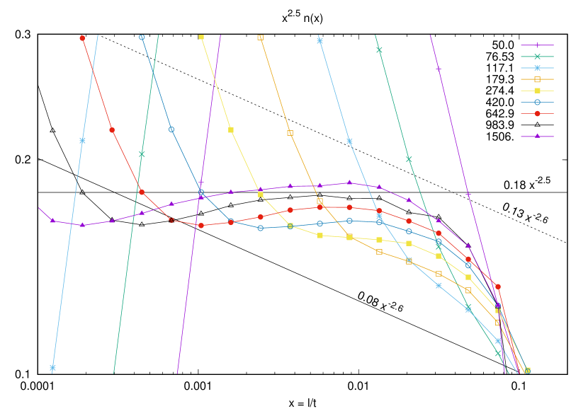
Figure 1: Loop densities in the radiation era at the conformal times listed, computed from five simulations of size 1500. The scaling loop density has been multiplied by $x^{2.5}$ to make small differences easier to see. The vertical scale ranges only over of a factor of 3 in loop density. Compare with more than 7 orders of magnitude in Fig. 3 of Ref. Ringeval et al. (2007) and 14 orders of magnitude in Fig. 9 of Ref. Blanco-Pillado et al. (2011).

shows our results for the radiation era. The colored lines with data points are the $n(x)$ found directly from our simulations. The horizontal black line is $n(x)=0.18x^{-2.5}$ as predicted by Eq. (63) of Ref. Blanco-Pillado et al. (2014). At the last time shown, the actual loop density is close to this line for loops whose lengths are in the range $10^{-3}$–$10^{-2}$. At larger sizes, we would not expect to this approximation to apply, because loops there have not yet been created. At smaller sizes, the loop density drops off slowly and then rises rapidly. The drop-off occurs because it takes time to approach a scaling regime. Scaling loops with $x=10^{-4}$ at conformal time 1500, for example, were primarily produced around time 150, when the network was much further from scaling and the production rate of large loops was less. The rapid rise at very small $x$ is an artifact of the initial conditions.

Even by time 1500, we have not reached a scaling loop density. The loop density takes longer to scale than the loop production function, because it is sensitive to loops produced in earlier eras further from scaling. For this reason we do not recommend using loop distributions to predict astrophysical signals. It is more accurate to extrapolate from the loop production function, as we did in Ref. Blanco-Pillado et al. (2014). We exhibit the directly determined loop distributions here only for comparison with prior work.

In Fig. 1 we see that the loop distribution has the same basic form for the last 3 or 4 timesteps shown. Before that there is a transient regime in which the loop distribution has a relatively straight segment rising more rapidly toward smaller loop sizes. This transient regime agrees reasonably well with the results of Ref. Ringeval et al. (2007). That paper was able to reach only conformal time 100. The slanted black line in Fig. 1 shows the central value of the extrapolated loop density determined there at the end of the run. This line runs mostly parallel to our result for time 179.3. The difference in normalization is of no consequence, because the error bars given in Ref. Ringeval et al. (2007) extend upward to the dashed line. The loop density was far from scaling at that time. Since we did not use the same initial conditions as Ref. Ringeval et al. (2007), we should not expect close agreement before scaling is reached. Nevertheless, one can see the general effect that times around 100 there is a steeper slope, but this is a transient that is replaced at later times by a curve with exponent around $-2.5$, falling off faster toward smaller sizes for the reason explained above.

A power law with $\beta=2.5$ lies within the error bars found by Ref. Ringeval et al. (2007). Thus our results here are consistent with their results. However, later work Lorenz et al. (2010); Abbott et al. (2018); Auclair et al. (2019a) based on Ref. Ringeval et al. (2007) used extrapolations applicable only for $\beta>2.5$. Such extrapolations are not justified by the larger simulations reported here.

III.2 Matter era

Figure 2

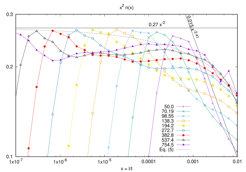
Figure 2: Loop densities in the matter era at the conformal times listed, computed from two simulations of size 750. The scaling loop density has been multiplied by $x^{2}$ to make small differences easier to see. The vertical scale ranges only over of a factor of 3 in loop density, compared with 6 orders of magnitude in Fig. 3 of Ref. Ringeval et al. (2007) and 11 orders of magnitude in Fig. 6 of Ref. Blanco-Pillado et al. (2011).

shows our results for the matter era. The situation is somewhat more complicated here because in the matter era the loop production is spread out over a wider range of loop sizes. The horizontal black line is $n(x)=0.27x^{-2}$, which is the asymptotic value for small loops predicted by Eq. (65) of Ref. Blanco-Pillado et al. (2014). The curved, dashed black line is

$$n(x)=0.27x^{-2}-0.45x^{-2.31}\,,$$ (5)

the entire prediction of the same equation without gravitational effects. We see that the directly computed loop density matches reasonably well to this line above about $x=3\times 10^{-5}$. For smaller loops there is a decline because loop production was not scaling at early times, and for much smaller loops a nonscaling rise associated with the initial conditions.

The sharply angled black line is the prediction of Ref. Ringeval et al. (2007) based on simulation data through conformal time 50 in units of the initial correlation length. Our simulations at time 50 agree very well with this distribution, but that is a transient regime, and the results at later times are of a different nature entirely. Taking account of the error bars in Eq. (2) does not produce much better agreement with the late-time data in Fig. 2.

III.3 Smoother initial conditions

In the simulations shown above the initial conditions consist of strings that go in straight segments between the centers of the Vachaspati-Vilenkin Vachaspati and Vilenkin (1984) plaquettes. One might be concerned that these strings are unnatural because they have significant kinks as they pass through the plaquette centers. To make sure that our results are not affected by such artifacts, we did some additional runs considering the string to be a quarter circle as it goes between two adjacent faces of a Vachaspati-Vilenkin cell. We then represented each quarter circle by 20 linear pieces. (If the string connects two opposite faces it is just a straight line, so there is no need to divide it.) Since these simulations have much more data than the ones with a single, straight segment between cube faces, we used we a smaller box and ran only until conformal time 420.

This division of circular segments into 20 smaller pieces corresponds roughly to the 20 “points per correlation length” used by Ref. Ringeval et al. (2007), but the ideas are not entirely the same. In our case, this choice affects the initial conditions only, but in Ref. Ringeval et al. (2007), the point spacing also affects the evolution of the network. Nevertheless, these runs may be more directly comparable to those of Ref. Ringeval et al. (2007).

The resulting loop density is shown in Fig. 3.

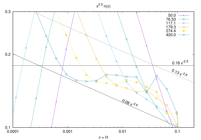
Figure 3: Loop densities in the radiation era computed from five simulations of size 400 with curved segments in the initial conditions represented in 20 pieces. The 6 times shown here are the same as the first 6 times in Fig. 1.

The results in this case are generally similar to those of Fig. 1, showing that the loop densities we find are not greatly influenced by the choice of straight rather than curved segments in the initial conditions.

IV Conclusions

In this work we extend the simulations of Ref. Ringeval et al. (2007) to determine the cosmic string loop density at conformal times a factor of 15 larger than the ones they reached. We find general agreement with Ref. Ringeval et al. (2007) at early times, but after that there is a different behavior that more closely approximates the $x^{-2.5}$ (radiation) $x^{-2}$ (matter) behavior expected for any loop production function that does not rise rapidly at small scales. It also agrees with the loop densities computed in Ref. Blanco-Pillado et al. (2014) starting from the loop production function. Given that agreement, it is better to determine the scaling loop production function and use that to compute the density, because the loop production function reaches scaling more quickly than the loop distribution Blanco-Pillado et al. (2011).

Both direct determination of loop density from simulation and extrapolation from the loop production function now give the same result that the loop density does not diverge faster at small sizes than $x^{-2.5}$ (radiation) $x^{-2}$ (matter). Thus there is no reason to consider loop densities with faster divergences such as “model 3” of Ref. Abbott et al. (2018).

The difference between $x^{-2.5}$ (radiation) $x^{-2}$ (matter) and more negative exponents has important observational consequences. Scaling distributions going as $x^{-2.5}$ (radiation) $x^{-2}$ (matter) may (and in our simulations do) consist primarily of loops produced at much earlier times. When gravitational effects are included, older loops are suppressed, leading to a flat spectrum at small scales. But more negative exponents can arise only from recently produced loops. Gravitational effects have had less time to act on such loops, so in such scenarios the loop distribution continues to grow toward small scales even when gravitation has been taken into account. (See Ref. Auclair et al. (2019b) for a detailed analysis.) This is the reason for the stronger bounds on cosmic strings found by Ref. Abbott et al. (2018) and different sensitivity predicted by Ref. Auclair et al. (2019a) in the case of “model 3”. But we see here that this analysis is based on a transient regime that does not persist in longer simulations.

References

- Kibble (1976) T. W. B. Kibble, “Topology of Cosmic Domains and Strings,” J. Phys. A9, 1387–1398 (1976).
- Vilenkin and Shellard (2000) A. Vilenkin and E. P. S. Shellard, Cosmic Strings and Other Topological Defects (Cambridge University Press, 2000).
- Dvali and Vilenkin (2004) Gia Dvali and Alexander Vilenkin, “Formation and evolution of cosmic D strings,” JCAP 0403, 010 (2004), arXiv:hep-th/0312007 [hep-th] .
- Copeland et al. (2004) Edmund J. Copeland, Robert C. Myers, and Joseph Polchinski, “Cosmic F and D strings,” JHEP 06, 013 (2004), arXiv:hep-th/0312067 [hep-th] .
- Damour and Vilenkin (2005) Thibault Damour and Alexander Vilenkin, “Gravitational radiation from cosmic (super)strings: Bursts, stochastic background, and observational windows,” Phys. Rev. D71, 063510 (2005), arXiv:hep-th/0410222 [hep-th] .
- Siemens et al. (2006) Xavier Siemens, Jolien Creighton, Irit Maor, Saikat Ray Majumder, Kipp Cannon, and Jocelyn Read, “Gravitational wave bursts from cosmic (super)strings: Quantitative analysis and constraints,” Phys. Rev. D73, 105001 (2006), arXiv:gr-qc/0603115 [gr-qc] .
- Sanidas et al. (2012) S. A. Sanidas, R. A. Battye, and B. W. Stappers, “Constraints on cosmic string tension imposed by the limit on the stochastic gravitational wave background from the European Pulsar Timing Array,” Phys. Rev. D85, 122003 (2012), arXiv:1201.2419 [astro-ph.CO] .
- Binetruy et al. (2012) Pierre Binetruy, Alejandro Bohe, Chiara Caprini, and Jean-Francois Dufaux, “Cosmological Backgrounds of Gravitational Waves and eLISA/NGO: Phase Transitions, Cosmic Strings and Other Sources,” JCAP 1206, 027 (2012), arXiv:1201.0983 [gr-qc] .
- Sousa and Avelino (2016) L. Sousa and P. P. Avelino, “Probing Cosmic Superstrings with Gravitational Waves,” Phys. Rev. D94, 063529 (2016), arXiv:1606.05585 [astro-ph.CO] .
- Kuroyanagi et al. (2012) Sachiko Kuroyanagi, Koichi Miyamoto, Toyokazu Sekiguchi, Keitaro Takahashi, and Joseph Silk, “Forecast constraints on cosmic string parameters from gravitational wave direct detection experiments,” Phys. Rev. D86, 023503 (2012), arXiv:1202.3032 [astro-ph.CO] .
- Blanco-Pillado and Olum (2017) Jose J. Blanco-Pillado and Ken D. Olum, “Stochastic gravitational wave background from smoothed cosmic string loops,” Phys. Rev. D96, 104046 (2017), arXiv:1709.02693 [astro-ph.CO] .
- Abbott et al. (2018) B. P. Abbott et al. (LIGO Scientific, Virgo), “Constraints on cosmic strings using data from the first Advanced LIGO observing run,” Phys. Rev. D97, 102002 (2018), arXiv:1712.01168 [gr-qc] .
- Auclair et al. (2019a) Pierre Auclair et al., “Probing the gravitational wave background from cosmic strings with LISA,” (2019a), arXiv:1909.00819 [astro-ph.CO] .
- Blanco-Pillado et al. (2018) Jose J. Blanco-Pillado, Ken D. Olum, and Xavier Siemens, “New limits on cosmic strings from gravitational wave observation,” Phys. Lett. B778, 392–396 (2018), arXiv:1709.02434 [astro-ph.CO] .
- Albrecht and Turok (1989) Andreas Albrecht and Neil Turok, “Evolution of Cosmic String Networks,” Phys. Rev. D40, 973–1001 (1989).
- Ringeval et al. (2007) Christophe Ringeval, Mairi Sakellariadou, and Francois Bouchet, “Cosmological evolution of cosmic string loops,” JCAP 0702, 023 (2007), arXiv:astro-ph/0511646 [astro-ph] .
- Vanchurin et al. (2006) Vitaly Vanchurin, Ken D. Olum, and Alexander Vilenkin, “Scaling of cosmic string loops,” Phys. Rev. D74, 063527 (2006), arXiv:gr-qc/0511159 [gr-qc] .
- Olum and Vanchurin (2007) Ken D. Olum and Vitaly Vanchurin, “Cosmic string loops in the expanding Universe,” Phys. Rev. D75, 063521 (2007), arXiv:astro-ph/0610419 [astro-ph] .
- Blanco-Pillado et al. (2011) Jose J. Blanco-Pillado, Ken D. Olum, and Benjamin Shlaer, “Large parallel cosmic string simulations: New results on loop production,” Phys. Rev. D83, 083514 (2011), arXiv:1101.5173 [astro-ph.CO] .
- Blanco-Pillado et al. (2014) Jose J. Blanco-Pillado, Ken D. Olum, and Benjamin Shlaer, “The number of cosmic string loops,” Phys. Rev. D89, 023512 (2014), arXiv:1309.6637 [astro-ph.CO] .
- Blanco-Pillado et al. (2019) Jose J. Blanco-Pillado, Ken D. Olum, and Jeremy M. Wachter, “Energy-conservation constraints on cosmic string loop production and distribution functions,” Phys. Rev. D100, 123526 (2019), arXiv:1907.09373 [astro-ph.CO] .
- Vachaspati and Vilenkin (1984) Tanmay Vachaspati and Alexander Vilenkin, “Formation and Evolution of Cosmic Strings,” Phys. Rev. D30, 2036 (1984).
- Lorenz et al. (2010) Larissa Lorenz, Christophe Ringeval, and Mairi Sakellariadou, “Cosmic string loop distribution on all length scales and at any redshift,” JCAP 1010, 003 (2010), arXiv:1006.0931 [astro-ph.CO] .
- Auclair et al. (2019b) Pierre Auclair, Christophe Ringeval, Mairi Sakellariadou, and Daniele Steer, “Cosmic string loop production functions,” JCAP 1906, 015 (2019b), arXiv:1903.06685 [astro-ph.CO] .