Optimal Dynamic Treatment Regimes
and Partial Welfare Ordering

Abstract

Dynamic treatment regimes are treatment allocations tailored to heterogeneous individuals. The optimal dynamic treatment regime is a regime that maximizes counterfactual welfare. We introduce a framework in which we can partially learn the optimal dynamic regime from observational data, relaxing the sequential randomization assumption commonly employed in the literature but instead using (binary) instrumental variables. We propose the notion of sharp partial ordering of counterfactual welfares with respect to dynamic regimes and establish mapping from data to partial ordering via a set of linear programs. We then characterize the identified set of the optimal regime as the set of maximal elements associated with the partial ordering. We relate the notion of partial ordering with a more conventional notion of partial identification using topological sorts. Practically, topological sorts can be served as a policy benchmark for a policymaker. We apply our method to understand returns to schooling and post-school training as a sequence of treatments by combining data from multiple sources. The framework of this paper can be used beyond the current context, e.g., in establishing rankings of multiple treatments or policies across different counterfactual scenarios.

JEL Numbers: C14, C32, C33, C36

Keywords: Optimal dynamic treatment regime, endogenous treatments, dynamic treatment effect, partial identification, instrumental variable, linear programming.

1 Introduction

Dynamic treatment regimes are dynamically personalized treatment allocations. Given that individuals are heterogeneous, allocations tailored to heterogeneity can improve overall welfare. Define a dynamic treatment regime $\boldsymbol{\delta}(\cdot)$ as a sequence of binary rules $\delta_{t}(\cdot)$ that map previous outcome and treatment (and possibly other covariates) onto current allocation decisions: $\delta_{t}(y_{t-1},d_{t-1})=d_{t}\in\{0,1\}$ for $t=1,...,T$. The motivation for being adaptive to the previous outcome is that it may contain information on unobserved heterogeneity that is not captured in covariates. Then the optimal dynamic treatment regime, which is this paper’s main parameter of interest, is defined as a regime that maximizes certain counterfactual welfare:

$$\boldsymbol{\delta}^{*}(\cdot) =\arg\max_{\boldsymbol{\delta}(\cdot)}W_{\boldsymbol{\delta}}.$$ (1.1)

This paper investigates the possibility of identifiability of the optimal dynamic regime $\boldsymbol{\delta}^{*}(\cdot)$ from data that are generated from randomized experiments in the presence of non-compliance or more generally from observational studies in multi-period settings.

Optimal treatment regimes have been extensively studied in the biostatistics literature (Murphy et al. (2001), Murphy (2003), and Robins (2004), among others). These studies typically rely on an ideal multi-stage experimental environment that satisfies sequential randomization. Based on such experimental data, they identify optimal regimes that maximize welfare, defined as the average counterfactual outcome. However, non-compliance is prevalent in experiments, and more generally, treatment endogeneity is a marked feature in observational studies. This may be one reason the vast biostatistics literature has not yet gained traction in other fields of social science, despite the potentially fruitful applications of optimal dynamic regimes in various policy evaluations.

To illustrate the policy relevance of the optimal dynamic regime, consider the labor market returns to high school education and post-school training for disadvantaged individuals. A policymaker may be interested in learning a schedule of allocation rules $\boldsymbol{\delta}(\cdot)=(\delta_{1},\delta_{2}(\cdot))$ that maximizes the employment rate $W_{\boldsymbol{\delta}}=E[Y_{2}(\boldsymbol{\delta})]$, where $\delta_{1}\in\{0,1\}$ assigns a high school diploma, $\delta_{2}(y_{1},\delta_{1})\in\{0,1\}$ assigns a job training program based on $\delta_{1}$ and earlier earnings $y_{1}\in\{0,1\}$ (low or high), and $Y_{2}(\boldsymbol{\delta})$ indicates the counterfactual employment status under regime $\boldsymbol{\delta}(\cdot)$. Suppose the optimal regime $\boldsymbol{\delta}^{*}(\cdot)$ is such that $\delta_{1}^{*}=1$, $\delta_{2}^{*}(0,\delta_{1}^{*})=1$, and $\delta_{2}^{*}(1,\delta_{1}^{*})=0$; that is, it turns out optimal to assign a high school diploma to all individuals and a training program to individuals with low earnings. One of the policy implications of such $\boldsymbol{\delta}^{*}(\cdot)$ is that the average job market performance can be improved by job trainings focusing on low performance individuals complementing with high school education. A static regime—where $\delta_{t}(\cdot)$ is a constant function—is a special case of a dynamic regime. In this sense, the optimal dynamic regime provides richer policy candidates than what can be learned from dynamic complementarity (Cunha and Heckman (2007), Cellini et al. (2010), Almond and Mazumder (2013), Johnson and Jackson (2019)). In learning $\boldsymbol{\delta}^{*}(\cdot)$ in this example, observational data may only be available where the observed treatments (schooling decisions) are endogenous.

This paper proposes a nonparametric framework, in which we can at least partially learn the ranking of counterfactual welfares $W_{\boldsymbol{\delta}}$’s and hence the optimal dynamic regime $\boldsymbol{\delta}^{*}(\cdot)$. We view that it is important to avoid making stringent modeling assumptions in the analysis of personalized treatments, because the core motivation of the analysis is individual heterogeneity, which we want to keep intact as much as possible. Instead, we embrace the partial identification approach. Given the observed distribution of sequences of outcomes and endogenous treatments and using the instrumental variable (IV) method, we establish sharp partial ordering of welfares, and characterize the identified set of optimal regimes as a discrete subset of all possible regimes. We define welfare as a linear functional of the joint distribution of counterfactual outcomes across periods. Examples of welfare include the average counterfactual terminal outcome commonly considered in the literature and as shown above. We assume we are equipped with some IVs that are possibly binary. We show that it is helpful to have a sequence of IVs generated from sequential experiments or quasi-experiments. Examples of the former are increasingly common as forms of random assignments or encouragements in medical trials, public health and educational interventions, and A/B testing on digital platforms. Examples of the latter can be some combinations of traditional IVs and regression discontinuity designs. Our framework also accommodates a single binary IV in the context of dynamic treatments and outcomes (e.g., Cellini et al. (2010)). The identifying power in such a case is investigated in simulation. The partial ordering and identified set proposed in this paper enable “sensitivity analyses.” That is, by comparing a chosen regime (e.g., from a parametric approach) with these benchmark objects, one can determine how much the former is led by assumptions and how much is informed by data. Such a practice also allows us to gain insight into data requirements to achieve a certain level of informativeness.

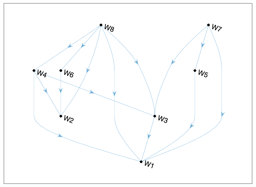
Figure 1: An Example of Sharp Partial Ordering of Welfares

The identification analysis is twofold. In the first part, we establish mapping from data to sharp partial ordering of counterfactual welfares with respect to possible regimes. The point identification of $\boldsymbol{\delta}^{*}(\cdot)$ will be achieved by establishing the total ordering of welfares, which is not generally possible in this flexible nonparametric framework with limited exogenous variation. Figure 1 is an example of partial ordering that we calculated by applying this paper’s theory and using simulated data. Here, we consider a two-period case as in the motivating example above, which yields eight possible $\boldsymbol{\delta}(\cdot)$’s and corresponding welfares, and “$\rightarrow$” corresponds to the relation “$>$”. To establish the partial ordering, we first characterize bounds on the difference between a pair of welfares as the set of optima of linear programs, and we do so for all possible welfare pairs. The bounds on welfare gaps are informative about whether welfares are comparable or not, and when they are, how to rank them. Then we show that although the bounds are calculated from separate optimizations, the partial ordering is consistent with common data-generating processes. The partial ordering obtained in this way is shown to be sharp in the sense that will become clear later. Note that each welfare gap measures the dynamic treatment effect. The partial ordering concisely (and tightly) summarizes the identified signs of these treatment effects, and thus can be a parameter of independent interest.

In the second part of the analysis, given the sharp partial ordering, we show that the identified set can be characterized as the set of maximal elements associated with the partial ordering, i.e., the set of regimes that are not inferior. For example, according to Figure 1, the identified set consists of regimes 7 and 8. Given the partial ordering, we also calculate topological sorts, which are total orderings that do not violate the underlying partial ordering. Theoretically, topological sorts can be viewed as observationally equivalent total orderings, which insight relates the partial ordering we consider with a more conventional notion of partial identification. Practically, topological sorts can be served as a policy benchmark that a policymaker can be equipped with. If desired, linear programming can be solved to calculate bounds on a small number of sorted welfares (e.g., top-tier welfares).

Given the minimal structure we impose in the data-generating process, the size of the identified set may be large in some cases. Such an identified set may still be useful in eliminating suboptimal regimes or warning about the lack of informativeness of the data. Often, however, researchers are willing to impose additional assumptions to gain identifying power. We propose identifying assumptions, such as uniformity assumptions that generalize the monotonicity assumption in Imbens and Angrist (1994), an assumption about an agent’s learning, Markovian structure, and stationarity. These assumptions tighten the identified set by reducing the dimension of the simplex in the linear programming, thus producing a denser partial ordering. We show that these assumptions are easy to impose in our framework.

This paper makes several contributions. To our best knowledge, this paper is first in the literature that considers the identifiability of optimal dynamic regimes under treatment endogeneity. The pioneering work by Murphy (2003) and subsequent works consider point identification of optimal dynamic regimes under the sequential randomization assumption. This paper brings this literature to observational contexts. Recently, Han (forthcoming), Han (2020), Cui and Tchetgen Tchetgen (2020), and Qiu et al. (2020) relax sequential randomization and establish identification of dynamic average treatment effects and/or optimal regimes using instrumental variables. In a single-period setup, they consider a regime that is a mapping only from covariates, but not previous outcomes and treatments, to an allocation. They focus on point identification by imposing assumptions such as the existence of additional exogenous variables in a multi-period setup (Han (forthcoming)), or the zero correlation between unmeasured confounders and compliance types (Cui and Tchetgen Tchetgen (2020); Qiu et al. (2020)) or uniformity (Han (2020)). The dynamic effects of treatment timing (i.e., irreversible treatments) have been considered in Heckman and Navarro (2007) and Heckman et al. (2016) who utilize exclusion restrictions and infinite support assumptions. A related staggered adoption design was recently studied in multi-period difference-in-differences settings under treatment heterogeneity by Athey and Imbens (2018), Callaway and Sant’Anna (2019), and Abraham and Sun (2020). This paper complements these papers by considering treatment scenarios of multiple dimensions with adaptivity as the key ingredient.

Second, this paper contributes to the literature on partial identification that utilizes linear programming approach, which has early examples as Balke and Pearl (1997) and Manski (2007), and appears recently in Torgovitsky (2019), Deb et al. (2017), Mogstad et al. (2018), Kitamura and Stoye (2019), Machado et al. (2019), Tebaldi et al. (2019), Kamat (2019), Gunsilius (2019), and Han and Yang (2020), to name a few. The advantages of this approach is that (i) bounds can be automatically obtained even when analytical derivation is not possible, (ii) the proof of sharpness is straightforward and not case-by-case, and (iii) it can streamline the analysis of different identifying assumptions. The dynamic framework of this paper complicates the identification analysis, which therefore fully benefits from these advantages. However, a distinct feature of the present paper is that the linear programming approach is used in establishing a sharp partial ordering across counterfactual objects—a novel concept in the literature—and in such a way that separate optimizations yield a common object, namely the partial ordering. The framework of this paper can also be useful in other settings where the goal is to compare welfares across multiple treatments and regimes—e.g., personalized treatment rules—or more generally, to establish rankings of policies across different counterfactual scenarios and find the best ones.

Third, we apply our method to conduct a policy analysis with schooling and post-school training as a sequence of treatments, which is to our knowledge a novel attempt in the literature. We consider dynamic treatment regimes of allocating a high school diploma and, given pre-program earnings, a job training program for economically disadvantaged population. By combining data from the Job Training Partnership Act (JTPA), the US Census, and the National Center for Education Statistics (NCES), we construct a data set with a sequence of instruments that is used to estimate the partial ordering of expected earnings and the identified set of the optimal regime. Even though only partial orderings are recovered, we can conclude with certainty that allocating the job training program only to the low earning type is welfare optimal. We also find that more costly regimes are not necessary welfare-improving.

The dynamic treatment regime considered in this paper is broadly related to the literature on statistical treatment rules, e.g., Manski (2004), Hirano and Porter (2009), Bhattacharya and Dupas (2012), Stoye (2012), Kitagawa and Tetenov (2018), Kasy (2016), and Athey and Wager (2017). However, our setting, assumptions, and goals are different from those in these papers. In a single-period setting, they consider allocation rules that map covariates to decisions. They impose assumptions that ensure point identification, such as (conditional) unconfoundedness, and focus on establishing the asymptotic optimality of the treatment rules, with Kasy (2016) the exception. Kasy (2016) focuses on establishing partial ranking by comparing a pair of treatment-allocating probabilities as policies. The notion of partial identification of ranking is related to ours, but we introduce the notion of sharpness of a partially ordered set with discrete policies and a linear programming approach to achieve that. Another distinction is that we consider a dynamic setup. Finally, in order to focus on the challenge with endogeneity, we consider a simple setup where the exploration and exploitation stages are separated, unlike in the literature on bandit problems (Kock and Thyrsgaard (2017), Kasy and Sautmann (forthcoming), Athey and Imbens (2019)). We believe the current setup is a good starting point.

In the next section, we introduce the dynamic regimes and related counterfactual outcomes, which define the welfare and the optimal regime. Section 3 provides a motivating example. Section 4 conducts the main identification analysis by constructing the partial ordering and characterizing the identified set. Sections 5–7 introduce topological sorts and additional identifying assumptions and discuss cardinality reduction for the set of regimes. Section 8 illustrates the analysis with numerical exercises, and Section 9 presents the empirical application on returns to schooling and job training. Finally, Section 10 concludes by discussing inference. Most proofs are collected in the Appendix.

In terms of notation, let $\boldsymbol{W}^{t}\equiv(W_{1},..,W_{t})$ denote a vector that collects r.v.’s $W_{t}$ across time up to $t$, and let $\boldsymbol{w}^{t}$ be its realization. Most of the time, we write $\boldsymbol{W}\equiv\boldsymbol{W}^{T}$ for convenience. We abbreviate “with probability one” as “w.p.1” and “with respect to” as “w.r.t.” The symbol “$\perp$” denotes statistical independence.

2 Dynamic Regimes and Counterfactual Welfares

2.1 Dynamic Regimes

Let $t$ be the index for a period or stage. For each $t=1,...,T$ with fixed $T$, define an adaptive treatment rule $\delta_{t}:\{0,1\}^{t-1}\times\{0,1\}^{t-1}\rightarrow\{0,1\}$ that maps the lags of the realized binary outcomes and treatments $\boldsymbol{y}^{t-1}\equiv(y_{1},...,y_{t-1})$ and $\boldsymbol{d}^{t-1}\equiv(d_{1},...,d_{t-1})$ onto a deterministic treatment allocation $d_{t}\in\{0,1\}$:

$$\delta_{t}(\boldsymbol{y}^{t-1},\boldsymbol{d}^{t-1}) =d_{t}.$$ (2.1)

This adaptive rule also appears in, e.g., Murphy (2003). The rule can also be a function of other discrete covariates, which is a straightforward extension and thus is not considered here for brevity. A special case of (2.1) is a static rule where $\delta_{t}(\cdot)$ is only a function of covariates but not $(\boldsymbol{y}^{t-1},\boldsymbol{d}^{t-1})$ (Han (forthcoming), Cui and Tchetgen Tchetgen (2020)) or a constant function. Binary outcomes and treatments are prevalent, and they are helpful in analyzing, interpreting, and implementing dynamic regimes (Zhang et al. (2015)). Still, extending the framework to allow for multi-valued discrete variables is possible. Whether the rule is dynamic or static, we only consider deterministic rules $\delta_{t}(\cdot)\in\{0,1\}$. In Appendix A.1, we extend this to stochastic rules $\tilde{\delta}_{t}(\cdot)\in[0,1]$ and show why it is enough to consider deterministic rules in some cases. Then, a dynamic regime up to period $t$ is defined as a vector of all treatment rules:

$$\boldsymbol{\delta}^{t}(\cdot) \equiv\left(\delta_{1},\delta_{2}(\cdot),...,\delta_{t}(\cdot)\right).$$

Let $\boldsymbol{\delta}(\cdot)\equiv\boldsymbol{\delta}^{T}(\cdot)\in\mathcal{D}$ where $\mathcal{D}$ is the set of all possible regimes. Throughout the paper, we will mostly focus on the leading case with $T=2$ for simplicity. Also, this case already captures the essence of the dynamic features, such as adaptivity and complementarity. Table 1 lists all possible dynamic regimes $\boldsymbol{\delta}(\cdot)\equiv\left(\delta_{1},\delta_{2}(\cdot)\right)$ as contingency plans.

Regime #	$\delta_{1}$	$\delta_{2}(1,\delta_{1})$	$\delta_{2}(0,\delta_{1})$
1	0	0	0
2	1	0	0
3	0	1	0
4	1	1	0
5	0	0	1
6	1	0	1
7	0	1	1
8	1	1	1

Table 1: Dynamic Regimes $\boldsymbol{\delta}(\cdot)$ When $T=2$

2.2 Counterfactual Welfares and Optimal Regimes

To define welfare w.r.t. this dynamic regime, we first introduce a counterfactual outcome as a function of a dynamic regime. Because of the adaptivity intrinsic in dynamic regimes, expressing counterfactual outcomes is more involved than that with static regimes $d_{t}$, i.e., $Y_{t}(\boldsymbol{d}^{t})$ with $\boldsymbol{d}^{t}\equiv(d_{1},...,d_{t})$. Let $\boldsymbol{Y}^{t}(\boldsymbol{d}^{t})\equiv(Y_{1}(d_{1}),Y_{2}(\boldsymbol{d}^{2}),...,Y_{t}(\boldsymbol{d}^{t}))$. We express a counterfactual outcome with adaptive regime $\boldsymbol{\delta}^{t}(\cdot)$ as follows:

$$Y_{t}(\boldsymbol{\delta}^{t}(\cdot)) \equiv Y_{t}(\boldsymbol{d}^{t}),$$ (2.2)

where the “bridge variables” $\boldsymbol{d}^{t}\equiv(d_{1},...,d_{t})$ satisfy

$$d_{1} =\delta_{1},$$

$$d_{2} =\delta_{2}(Y_{1}(d_{1}),d_{1}),$$

$$d_{3} =\delta_{3}(\boldsymbol{Y}^{2}(\boldsymbol{d}^{2}),\boldsymbol{d}^{2}),$$ (2.3)

$$\vdots$$

$$d_{t} =\delta_{t}(\boldsymbol{Y}^{t-1}(\boldsymbol{d}^{t-1}),\boldsymbol{d}^{t-1}).$$

Suppose $T=2$. Then, the two counterfactual outcomes are defined as $Y_{1}(\delta_{1})=Y_{1}(d_{1})$ and $Y_{2}(\boldsymbol{\delta}^{2}(\cdot))=Y_{2}(\delta_{1},\delta_{2}(Y_{1}(\delta_{1}),\delta_{1}))$.

Let $q_{\boldsymbol{\delta}}(\boldsymbol{y})\equiv\Pr[\boldsymbol{Y}(\boldsymbol{\delta}(\cdot))=\boldsymbol{y}]$ be the joint distribution of counterfactual outcome vector $\boldsymbol{Y}(\boldsymbol{\delta}(\cdot))\equiv(Y_{1}(\delta_{1}),Y_{2}(\boldsymbol{\delta}^{2}(\cdot)),...,Y_{T}(\boldsymbol{\delta}(\cdot)))$. We define counterfactual welfare as a linear functional of $q_{\boldsymbol{\delta}}(\boldsymbol{y})$:

$$W_{\boldsymbol{\delta}} \equiv f(q_{\boldsymbol{\delta}}).$$

Examples of the functional include the average counterfactual terminal outcome $E[Y_{T}(\boldsymbol{\delta}(\cdot))]=\Pr[Y_{T}(\boldsymbol{\delta}(\cdot))=1]$, our leading case and which is common in the literature, and the weighted average of counterfactuals $\sum_{t=1}^{T}\omega_{t}E[Y_{t}(\boldsymbol{\delta}^{t}(\cdot))]$. Then, the optimal dynamic regime is a regime that maximizes the welfare as defined in (1.1):

$$\boldsymbol{\delta}^{*}(\cdot) =\arg\max_{\boldsymbol{\delta}(\cdot)\in\mathcal{D}}W_{\boldsymbol{\delta}}.$$

In the case of $W_{\boldsymbol{\delta}}=E[Y_{T}(\boldsymbol{\delta}(\cdot))]$, the solution $\boldsymbol{\delta}^{*}(\cdot)$ can be justified by backward induction in finite-horizon dynamic programming. Moreover in this case, the regime with deterministic rules $\delta_{t}(\cdot)\in\{0,1\}$ achieves the same optimal regime and optimized welfare as the regime with stochastic rules $\delta_{t}(\cdot)\in[0,1]$; see Theorem A.1 in Appendix A.1.

The identification analysis of the optimal regime is closely related to the identification of welfare for each regime and welfare gaps, which also contain information for policy. Some interesting special cases are the following: (i) the optimal welfare, $W_{\boldsymbol{\delta}^{*}}$, which in turn yields (ii) the regret from following individual decisions, $W_{\boldsymbol{\delta}^{*}}-W_{\boldsymbol{D}}$, where $W_{\boldsymbol{D}}$ is simply $f(\Pr[\boldsymbol{Y}(\boldsymbol{D})=\cdot])=f(\Pr[\boldsymbol{Y}=\cdot])$, and (iii) the gain from adaptivity, $W_{\boldsymbol{\delta}^{*}}-W_{\boldsymbol{d}^{*}}$, where $W_{\boldsymbol{d}^{*}}=\max_{\boldsymbol{d}}W_{\boldsymbol{d}}$ is the optimum of the welfare with a static rule, $W_{\boldsymbol{d}}=f(\Pr[\boldsymbol{Y}(\boldsymbol{d})=\cdot])$. If the cost of treatments is not considered, the gain in (iii) is non-negative as the set of all $\boldsymbol{d}$ is a subset of $\mathcal{D}$.

3 Motivating Examples

For illustration, we continue discussing the example in the Introduction. This stylized example in an observational setting is meant to motivate the policy relevance of the optimal dynamic regime and the type of data that are useful for recovering it. Again, consider labor market returns to high school education and post-school training for disadvantaged individuals. Let $D_{i1}=1$ if student $i$ has a high school diploma and $D_{i1}=0$ otherwise; let $D_{i2}=1$ if $i$ participates in a job training program and $D_{i2}=0$ if not. Also, let $Y_{i1}=1$ if $i$ is employed before the training program and $Y_{i1}=0$ if not; let $Y_{i2}=1$ if $i$ is employed after the program and $Y_{i2}=0$ if not. Given the data, suppose we are interested in recovering regimes that maximize the employment rate as welfare.

First, consider a static regime, which is a schedule $\boldsymbol{d}=(d_{1},d_{2})\in\{0,1\}^{2}$ of first assigning a high school diploma ($d_{1}\in\{0,1\}$) and then a job training ($d_{2}\in\{0,1\}$). Define associated welfare, which is the employment rate $W_{\boldsymbol{d}}=E[Y_{2}(\boldsymbol{d})]$. This setup is already useful in learning, for example, $E[Y_{2}(1,0)]-E[Y_{2}(0,1)]$ or complementarity (i.e., $E[Y_{2}(0,1)]-E[Y_{2}(0,0)]$ versus $E[Y_{2}(1,1)]-E[Y_{2}(1,0)]$), which cannot be learned from period-specific treatment effects. However, because $d_{1}$ and $d_{2}$ are not simultaneously given but $d_{1}$ precedes $d_{2}$, the allocation $d_{2}$ can be more informed by incorporating the knowledge about the individual’s response $y_{1}$ to $d_{1}$. This motivates the dynamic regime, which is the schedule $\boldsymbol{\delta}(\cdot)=(\delta_{1},\delta_{2}(\cdot))\in\mathcal{D}$ of allocation rules that first assigns a high school diploma ($\delta_{1}\in\{0,1\}$) and then a job training ($\delta_{2}(y_{1},\delta_{1})\in\{0,1\}$) depending on $\delta_{1}$ and the employment status $y_{1}$. Then, the optimal regime with adaptivity $\boldsymbol{\delta}^{*}(\cdot)$ is the one that maximizes $W_{\boldsymbol{\delta}}=E[Y_{2}(\boldsymbol{\delta})]$. As argued in the Introduction, $\boldsymbol{\delta}^{*}(\cdot)$ provides policy implications that $\boldsymbol{d}^{*}$ cannot.

As $D_{1}$ and $D_{2}$ are endogenous, $\{D_{i1},Y_{i1},D_{i2},Y_{i2}\}$ above are not useful by themselves to identify $W_{\boldsymbol{\delta}}$’s and $\boldsymbol{\delta}^{*}(\cdot)$. We employ the approach of using IVs, either a single IV (e.g., in the initial period) or a sequence of IVs. In experimental settings, examples of a sequence of IVs can be found in multi-stage experiments, such as the Fast Track Prevention Program (Conduct Problems Prevention Research Group (1992)), the Elderly Program randomized trial for the Systolic Hypertension (The Systolic Hypertension in the Elderly Program (SHEP) Cooperative Research Group (1988)), and Promotion of Breastfeeding Intervention Trial (Kramer et al. (2001)). It is also possible to combine multiple experiments as in Johnson and Jackson (2019). In observational settings, one can use IVs from quasi-experiments, those from RD design, or a combination of them. In the example above, we can use the distance to high schools or the number of high schools per square mile as an instrument $Z_{1}$ for $D_{1}$. Then, a random assignment of the job training in a field experiment can be used as an instrument $Z_{2}$ for the compliance decision $D_{2}$. In fact, in Section 9, we study schooling and job training as a sequence of treatments and combine IVs from experimental and observational data.

4 Partial Ordering and Partial Identification

4.1 Observables

We introduce observables based on which we want to identify the optimal regime and counterfactual welfares. Assume that the time length of the observables is equal to $T$, the length of the optimal regime to be identified. For each period or stage $t=1,...,T$, assume that we observe the binary instrument $Z_{t}$, the binary endogenous treatment decision $D_{t}$, and the binary outcome $Y_{t}=\sum_{\boldsymbol{d}^{t}\in\{0,1\}^{t}}1\{\boldsymbol{D}^{t}=\boldsymbol{d}^{t}\}Y_{t}(\boldsymbol{d}^{t})$. These variables are motivated in the previous section. As another example, $Y_{t}$ is a symptom indicator for a patient, $D_{t}$ is the medical treatment received, and $Z_{t}$ is generated by a multi-period medical trial. Importantly, the framework does not preclude the case in which $Z_{t}$ exists only for some $t$ but not all; see Section 8 for related discussions. In this case, $Z_{t}$ for the other periods is understood to be degenerate. Let $D_{t}(\boldsymbol{z}^{t})$ be the counterfactual treatment given $\boldsymbol{z}^{t}\equiv(z_{1},...,z_{t})\in\{0,1\}^{t}$. Then, $D_{t}=\sum_{\boldsymbol{z}^{t}\in\mathcal{Z}^{t}}D_{t}(\boldsymbol{z}^{t})$. Let $\boldsymbol{Y}(\boldsymbol{d})\equiv(Y_{1}(d_{1}),Y_{2}(\boldsymbol{d}^{2}),...,Y_{T}(\boldsymbol{d}))$ and $\boldsymbol{D}(\boldsymbol{z})\equiv(D_{1}(z_{1}),D_{2}(\boldsymbol{z}^{2}),...,D_{T}(\boldsymbol{z}))$.

Assumption SX.

$Z_{t}\perp(\boldsymbol{Y}(\boldsymbol{d}),\boldsymbol{D}(\boldsymbol{z}))|\boldsymbol{Z}^{t-1}$.

Assumption SX assumes the strict exogeneity and exclusion restriction. A single IV with full independence trivially satisfies this assumption. For a sequence of IVs, this assumption is satisfied in typical sequential randomized experiments, as well as quasi-experiments as discussed in Section 3. Let $(\boldsymbol{Y},\boldsymbol{D},\boldsymbol{Z})$ be the vector of observables $(Y_{t},D_{t},Z_{t})$ for the entire $T$ periods and let $p$ be its distribution. We assume that $(\boldsymbol{Y}_{i},\boldsymbol{D}_{i},\boldsymbol{Z}_{i})$ is independent and identically distributed and $\{(\boldsymbol{Y}_{i},\boldsymbol{D}_{i},\boldsymbol{Z}_{i}):i=1,...,N\}$ is a small $T$ large $N$ panel. We mostly suppress the individual unit $i$ throughout the paper. For empirical applications, the data structure can be more general than a panel and the kinds of $Y_{t}$, $D_{t}$ and $Z_{t}$ are allowed to be different across time; Section 3 contains such an example. For the population from which the data are drawn, we are interested in learning the optimal regime.

4.2 Partial Ordering of Welfares

Given the distribution $p$ of the data $(\boldsymbol{Y},\boldsymbol{D},\boldsymbol{Z})$ and under Assumption SX, we show how the optimal dynamic regime and welfares can be partially recovered. The identified set of $\boldsymbol{\delta}^{*}(\cdot)$ will be characterized as a subset of the discrete set $\mathcal{D}$. As the first step, we establish partial ordering of $W_{\boldsymbol{\delta}}$ w.r.t. $\boldsymbol{\delta}(\cdot)\in\mathcal{D}$ as a function of $p$. The partial ordering summarizes the identified signs of the dynamic treatment effects, as will become clear later. The partial ordering can be represented by a directed acyclic graph (DAG). The DAG representation is fruitful for introducing the notion of the sharpness of partial ordering and later to translate it into the identified set of $\boldsymbol{\delta}^{*}(\cdot)$.

To facilitate this analysis, we enumerate all $\left|\mathcal{D}\right|=2^{2^{T}-1}$ possible regimes. For index $k\in\mathcal{K}\equiv\{k:1\leq k\leq\left|\mathcal{D}\right|\}$ (and thus $\left|\mathcal{K}\right|=\left|\mathcal{D}\right|$), let $\boldsymbol{\delta}_{k}(\cdot)$ denote the $k$-th regime in $\mathcal{D}$. For $T=2$, Table 1 indexes all possible dynamic regimes $\boldsymbol{\delta}(\cdot)\equiv\left(\delta_{1},\delta_{2}(\cdot)\right)$. Let $W_{k}\equiv W_{\boldsymbol{\delta}_{k}}$ be the corresponding welfare. Figure 2 illustrates examples of the partially ordered set of welfares where each edge “$W_{k}\rightarrow W_{k^{\prime}}$” indicates the relation “$W_{k}>W_{k^{\prime}}$.”

(a) $\boldsymbol{\delta}^{*}(\cdot)$ is partially identified

(b) $\boldsymbol{\delta}^{*}(\cdot)$ is point identified

Figure 2: Partially Ordered Sets of Welfares

In general, the point identification of $\boldsymbol{\delta}^{*}(\cdot)$ is achieved by establishing the total ordering of $W_{k}$, which is not possible with instruments of limited support. Instead, we only recover a partial ordering. We want the partial ordering to be sharp in the sense that it cannot be improved given the data and maintained assumptions. To formally state this, let $G(\mathcal{K},\mathcal{E})$ be a DAG where $\mathcal{K}$ is the set of welfare (or regime) indices and $\mathcal{E}$ is the set of edges.

Definition 4.1.

Given the data distribution $p$, a partial ordering $G(\mathcal{K},\mathcal{E}_{p})$ is sharp under the maintained assumptions if there exists no partial ordering $G(\mathcal{K},\mathcal{E}_{p}^{\prime})$ such that $\mathcal{E}_{p}^{\prime}\supsetneq\mathcal{E}_{p}$ without imposing additional assumptions.

Establishing sharp partial ordering amounts to determining whether we can tightly identify the sign of a counterfactual welfare gap $W_{k}-W_{k^{\prime}}$ (i.e., the dynamic treatment effects) for $k,k^{\prime}\in\mathcal{K}$, and if we can, what the sign is.

4.3 Data-Generating Framework

We introduce a simple data-generating framework and formally define the identified set. First, we introduce latent state variables that generate $(\boldsymbol{Y},\boldsymbol{D})$. A latent state of the world will determine specific maps $(\boldsymbol{y}^{t-1},\boldsymbol{d}^{t})\mapsto y_{t}$ and $(\boldsymbol{y}^{t-1},\boldsymbol{d}^{t-1},\boldsymbol{z}^{t})\mapsto d_{t}$ for $t=1,...,T$ under the exclusion restriction in Assumption SX. We introduce the latent state variable $\tilde{S}_{t}$ whose realization represents such a state. We define $\tilde{S}_{t}$ as follows. For given $(\boldsymbol{y}^{t-1},\boldsymbol{d}^{t},\boldsymbol{z}^{t})$, let $Y_{t}(\boldsymbol{y}^{t-1},\boldsymbol{d}^{t})$ and $D_{t}(\boldsymbol{y}^{t-1},\boldsymbol{d}^{t-1},\boldsymbol{z}^{t})$ denote the extended counterfactual outcomes and treatments, respectively, and let $\{Y_{t}(\boldsymbol{y}^{t-1},\boldsymbol{d}^{t})\}$ and $\{D_{t}(\boldsymbol{y}^{t-1},\boldsymbol{d}^{t-1},\boldsymbol{z}^{t})\}$ and their sequences w.r.t. $(\boldsymbol{y}^{t-1},\boldsymbol{d}^{t},\boldsymbol{z}^{t})$. Then, by concatenating the two sequences, define $\tilde{S}_{t}\equiv(\{Y_{t}(\boldsymbol{y}^{t-1},\boldsymbol{d}^{t})\},\{D_{t}(\boldsymbol{y}^{t-1},\boldsymbol{d}^{t-1},\boldsymbol{z}^{t})\})\in\{0,1\}^{2^{2t-1}}\times\{0,1\}^{2^{3t-2}}$. For example, $\tilde{S}_{1}=(Y_{1}(0),Y_{1}(1),D_{1}(0),D_{1}(1))\in\{0,1\}^{2}\times\{0,1\}^{2}$, whose realization specifies particular maps $d_{1}\mapsto y_{1}$ and $z_{1}\mapsto d_{1}$. It is convenient to transform $\tilde{\boldsymbol{S}}\equiv(\tilde{S}_{1},...,\tilde{S}_{T})$ into a scalar (discrete) latent variable in $\mathbb{N}$ as $S\equiv\beta(\tilde{\boldsymbol{S}})\in\mathcal{S}\subset\mathbb{N}$, where $\beta(\cdot)$ is a one-to-one map that transforms a binary sequence into a decimal value. Define

$$q_{s} \equiv\Pr[S=s],$$

and define the vector $q$ of $q_{s}$ which represents the distribution of $S$, namely the true data-generating process. The vector $q$ resides in $\mathcal{Q}\equiv\{q:\sum_{s}q_{s}=1\text{ and }q_{s}\geq 0\text{ }\forall s\}$ of dimension $d_{q}-1$ where $d_{q}\equiv\dim(q)$. A useful fact is that the joint distribution of counterfactuals can be written as a linear functional of $q$:

$$\Pr[\boldsymbol{Y}(\boldsymbol{d})=\boldsymbol{y},\boldsymbol{D}(\boldsymbol{z})=\boldsymbol{d}] =\Pr[S\in\mathcal{S}:\boldsymbol{Y}(\boldsymbol{y}^{T-1},\boldsymbol{d})=\boldsymbol{y},\boldsymbol{D}(\boldsymbol{y}^{T-1},\boldsymbol{d}^{T-1},\boldsymbol{z})=\boldsymbol{d}]$$

$$=\Pr[S\in\mathcal{S}:Y_{t}(\boldsymbol{y}^{t-1},\boldsymbol{d}^{t})=y_{t},D_{t}(\boldsymbol{y}^{t-1},\boldsymbol{d}^{t-1},\boldsymbol{z}^{t})=d_{t}\quad\forall t]$$

$$=\sum_{s\in\mathcal{S}_{\boldsymbol{y},\boldsymbol{d}|\boldsymbol{z}}}q_{s},$$ (4.1)

where $\mathcal{S}_{\boldsymbol{y},\boldsymbol{d}|\boldsymbol{z}}$ is constructed by using the definition of $S$; its expression can be found in Appendix A.2.

Based on (4.1), the counterfactual welfare can be written as a linear combination of $q_{s}$’s. That is, there exists $1\times d_{q}$ vector $A_{k}$ of $1$’s and $0$’s such that

$$W_{k} =A_{k}q.$$ (4.2)

The formal derivation of $A_{k}$ can be found in Appendix A.2, but the intuition is as follows. Recall $W_{k}\equiv f(q_{\boldsymbol{\delta}_{k}})$ where $q_{\boldsymbol{\delta}}(\boldsymbol{y})\equiv\Pr[\boldsymbol{Y}(\boldsymbol{\delta}(\cdot))=\boldsymbol{y}]$. The key observation in deriving the result (4.2) is that $\Pr[\boldsymbol{Y}(\boldsymbol{\delta}(\cdot))=\boldsymbol{y}]$ can be written as a linear functional of the joint distributions of counterfactual outcomes with a static regime, i.e., $\Pr[\boldsymbol{Y}(\boldsymbol{d})=\boldsymbol{y}]$’s, which in turn is a linear functional of $q$. To illustrate with $T=2$ and welfare $W_{\boldsymbol{\delta}}=E[Y_{2}(\boldsymbol{\delta}(\cdot))]$, we have

$$\Pr[Y_{2}(\boldsymbol{\delta}(\cdot))=1] =\sum_{y_{1}\in\{0,1\}}\Pr[Y_{2}(\delta_{1},\delta_{2}(Y_{1}(\delta_{1}),\delta_{1}))=1|Y_{1}(\delta_{1})=y_{1}]\Pr[Y_{1}(\delta_{1})=y_{1}]$$

by the law of iterated expectation. Then, for instance, Regime 4 in Table 1 yields

$$\Pr[Y_{2}(\boldsymbol{\delta}_{4}(\cdot))=1] =P[\boldsymbol{Y}(1,1)=(1,1)]+P[\boldsymbol{Y}(1,0)=(0,1)],$$ (4.3)

where each $\Pr[\boldsymbol{Y}(d_{1},d_{2})=(y_{1},y_{2})]$ is the counterfactual distribution with a static regime, which in turn is a linear functional of (4.1).

The data impose restrictions on $q\in\mathcal{Q}$. Define

$$p_{\boldsymbol{y},\boldsymbol{d}|\boldsymbol{z}} \equiv p(\boldsymbol{y},\boldsymbol{d}|\boldsymbol{z})\equiv\Pr[\boldsymbol{Y}=\boldsymbol{y},\boldsymbol{D}=\boldsymbol{d}|\boldsymbol{Z}=\boldsymbol{z}],$$

and $p$ as the vector of $p_{\boldsymbol{y},\boldsymbol{d}|\boldsymbol{z}}$’s except redundant elements. Let $d_{p}\equiv\dim(p)$. Since $\Pr[\boldsymbol{Y}=\boldsymbol{y},\boldsymbol{D}=\boldsymbol{d}|\boldsymbol{Z}=\boldsymbol{z}]=\Pr[\boldsymbol{Y}(\boldsymbol{d})=\boldsymbol{y},\boldsymbol{D}(\boldsymbol{z})=\boldsymbol{d}]$ by Assumption SX, we can readily show by (4.1) that there exists $d_{p}\times d_{q}$ matrix $B$ such that

$$Bq =p,$$ (4.4)

where each row of $B$ is a vector of $1$’s and $0$’s; the formal derivation of $B$ can be found in Appendix A.2. It is worth noting that the linearity in (4.2) and (4.4) is not a restriction but given by the discrete nature of the setting. We assume $rank(B)=d_{p}$ without loss of generality, because redundant constraints do not play a role in restricting $\mathcal{Q}$. We focus on the non-trivial case of $d_{p}<d_{q}$. If $d_{p}\geq d_{q}$, which is rare, we can solve for $q=(B^{\top}B)^{-1}B^{\top}p$, and can trivially point identify $W_{k}=A_{k}q$ and thus $\boldsymbol{\delta}^{*}(\cdot)$. Otherwise, we have a set of observationally equivalent $q$’s, which is the source of partial identification and motivates the following definition of the identified set.

For a given $q$, let $\boldsymbol{\delta}^{*}(\cdot;q)\equiv\arg\max_{\boldsymbol{\delta}_{k}(\cdot)\in\mathcal{D}}W_{k}=A_{k}q$ be the optimal regime, explicitly written as a function of the data-generating process.

Definition 4.2.

Under Assumption SX, the identified set of $\boldsymbol{\delta}^{*}(\cdot)$ given the data distribution $p$ is

$$\mathcal{D}_{p}^{*} \equiv\{\boldsymbol{\delta}^{*}(\cdot;q):Bq=p\text{ and }q\in\mathcal{Q}\}\subset\mathcal{D},$$ (4.5)

which is assumed to be empty when $Bq\neq p$.

4.4 Characterizing Partial Ordering and the Identified Set

Given $p$, we establish the partial ordering of $W_{k}$’s by determining whether $W_{k}>W_{k^{\prime}}$, $W_{k}<W_{k^{\prime}}$, or $W_{k}$ and $W_{k^{\prime}}$ are not comparable (including $W_{k}=W_{k^{\prime}}$), denoted as $W_{k}\sim W_{k^{\prime}}$, for $k,k^{\prime}\in\mathcal{K}$. As described in the next theorem, this procedure can be accomplished by determining the signs of the bounds on the welfare gap $W_{k}-W_{k^{\prime}}$ for $k,k^{\prime}\in\mathcal{K}$ and $k>k^{\prime}$. Then the identified set can be characterized based on the resulting partial ordering.

The nature of the data generation induces the linear system (4.2) and (4.4). This enables us to characterize the bounds on $W_{k}-W_{k^{\prime}}=(A_{k}-A_{k^{\prime}})q$ as the optima in linear programming. Let $U_{k,k^{\prime}}$ and $L_{k,k^{\prime}}$ be the upper and lower bounds. Also let $\Delta_{k,k^{\prime}}\equiv A_{k}-A_{k^{\prime}}$ for simplicity, and thus the welfare gap is expressed as $W_{k}-W_{k^{\prime}}=\Delta_{k,k^{\prime}}q$. Then, for $k,k^{\prime}\in\mathcal{K}$, we have the main linear programs:

$$\begin{array}[]{c}U_{k,k^{\prime}}=\max_{q\in\mathcal{Q}}\Delta_{k,k^{\prime}}q,\\ L_{k,k^{\prime}}=\min_{q\in\mathcal{Q}}\Delta_{k,k^{\prime}}q,\end{array} \qquad s.t.\quad Bq=p.$$ (4.8)

Assumption B.

$\{q:Bq=p\}\cap\mathcal{Q}\neq\emptyset$.

Assumption B imposes that the model, Assumption SX in this case, is correctly specified. Under misspecification, the identified set is empty by definition. The next theorem constructs the sharp partial ordering and characterize the identified set using $U_{k,k^{\prime}}$ and $L_{k,k^{\prime}}$ for $k,k^{\prime}\in\mathcal{K}$ and $k>k^{\prime}$, or equivalently, $L_{k,k^{\prime}}$ for $k,k^{\prime}\in\mathcal{K}$ and $k\neq k^{\prime}$.

Theorem 4.1.

Suppose Assumptions SX and B hold. Then, (i) $G(\mathcal{K},\mathcal{E}_{p})$ with $\mathcal{E}_{p}\equiv\{(k,k^{\prime})\in\mathcal{K}:L_{k,k^{\prime}}>0\text{ and }k\neq k^{\prime}\}$ is sharp; (ii) $\mathcal{D}_{p}^{*}$ defined in (4.5) satisfies

$$\mathcal{D}_{p}^{*} =\{\boldsymbol{\delta}_{k^{\prime}}(\cdot):\nexists k\in\mathcal{K}\text{ such that }L_{k,k^{\prime}}>0\text{ and }k\neq k^{\prime}\}$$ (4.9)

$$=\{\boldsymbol{\delta}_{k^{\prime}}(\cdot):L_{k,k^{\prime}}\leq 0\text{ for all }k\in\mathcal{K}\text{ and }k\neq k^{\prime}\},$$ (4.10)

and therefore the sets on the right-hand side are sharp.

The proof of Theorem 4.1 is shown in the Appendix. The key insight of the proof is that even though the bounds on the welfare gaps are calculated from separate optimizations, the partial ordering is governed by common $q$’s (each of which generates all the welfares) that are observationally equivalent; see Section 5.2 for related discussions.

Theorem 4.1(i) prescribes how to calculate the sharp partial ordering as a function of data. According to (4.9) in (ii), $\mathcal{D}_{p}^{*}$ is characterized as the collection of $\boldsymbol{\delta}_{k}(\cdot)$ where $k$ is in the set of maximal elements of the partially ordered set $G(\mathcal{K},\mathcal{E}_{p})$, i.e., the set of regimes that are not inferior. In Figure 2, it is easy to see that the set of maximals is $\mathcal{D}_{p}^{*}=\{\boldsymbol{\delta}_{1}(\cdot),\boldsymbol{\delta}_{4}(\cdot)\}$ in panel (a) and $\mathcal{D}_{p}^{*}=\{\boldsymbol{\delta}_{1}(\cdot)\}$ in panel (b).

The identified set $\mathcal{D}_{p}^{*}$ characterizes the information content of the model. Given the minimal structure we impose in the model, $\mathcal{D}_{p}^{*}$ may be large in some cases. However, we argue that an uninformative $\mathcal{D}_{p}^{*}$ still has implications for policy: (i) such set may recommend the policymaker eliminate sub-optimal regimes from her options; (ii) in turn, it warns the policymaker about her lack of information (e.g., even if she has access to the experimental data); when $\mathcal{D}_{p}^{*}=\mathcal{D}$ as one extreme, “no recommendation” can be given as a non-trivial policy suggestion of the need for better data. As shown in the numerical exercise, the size of $\mathcal{D}_{p}^{*}$ is related to the strength of $Z_{t}$ (i.e., the size of the complier group at $t$) and the strength of the dynamic treatment effects. This is reminiscent of the findings in Machado et al. (2019) for the average treatment effect in a static model. In Section 6, we list further identifying assumptions that help shrink $\mathcal{D}_{p}^{*}$.

5 Set of the $n$-th Best Regimes, Topological Sorts, and Bounds on Sorted Welfare

In this section, we propose some ways to report results of this paper including the partial ordering. These approaches can be useful especially when the obtained partial ordering is complicated (e.g., with a longer horizon).

5.1 Set of the $n$-th Best Policies

When the partial ordering of welfare is the parameter of interest, the identified set of $\boldsymbol{\delta}^{*}(\cdot)$ can be viewed as a summary of the partial ordering. This view can be extended to introduce a set of the $n$-th best regimes, which further summarizes the partial ordering. With slight abuse of notation, we can formalize it as follows.

Recall $\mathcal{K}$ is the set of all regime indices. Motivated from (4.9), let $\mathcal{K}_{p}^{(1)}\equiv\{k^{\prime}:\nexists k\in\mathcal{K}\text{ such that }L_{k,k^{\prime}}>0\text{ and }k\neq k^{\prime}\in\mathcal{K}\}$ be the set of maximal elements of the partial ordering and let $\mathcal{D}_{p}^{(1)}\equiv\{\boldsymbol{\delta}_{k^{\prime}}(\cdot):k^{\prime}\in\mathcal{K}_{p}^{(1)}\}$. Theorem 4.1(ii) can be simply stated as $\mathcal{D}_{p}^{*}=\mathcal{D}_{p}^{(1)}$. To define the set of second-best regimes, we first remove all the elements in $\mathcal{K}_{p}^{(1)}$ from the set of candidate. Accordingly, by defining

$$\mathcal{K}_{p}^{(2)} \equiv\{k^{\prime}:\nexists k\in\mathcal{K}\backslash\mathcal{K}_{p}^{(1)}\text{ such that }L_{k,k^{\prime}}>0\text{ and }k\neq k^{\prime}\in\mathcal{K}\backslash\mathcal{K}_{p}^{(1)}\},$$

we can introduce the set of second-best regimes: $\mathcal{D}_{p}^{(2)}\equiv\{\boldsymbol{\delta}_{k^{\prime}}(\cdot):k^{\prime}\in\mathcal{K}_{p}^{(2)}\}$. Iteratively, we can define the set of $n$-th best regimes as $\mathcal{D}_{p}^{(n)}\equiv\{\boldsymbol{\delta}_{k^{\prime}}(\cdot):k^{\prime}\in\mathcal{K}_{p}^{(n)}\}$ where

$$\mathcal{K}_{p}^{(n)} =\left\{k^{\prime}:\nexists k\in\mathcal{K}\backslash\bigcup_{j=1}^{n-1}\mathcal{K}_{p}^{(j)}\text{ such that }L_{k,k^{\prime}}>0\text{ and }k\neq k^{\prime}\in\mathcal{K}\backslash\bigcup_{j=1}^{n-1}\mathcal{K}_{p}^{(j)}\right\}.$$

The sets $\mathcal{D}_{p}^{(1)},...,\mathcal{D}_{p}^{(n)}$ are useful policy benchmarks. For instance, the policy maker can conduct a sensitivity analysis for her chosen regime (e.g., from a parametric model) by inspecting in which set the regime is contained.

5.2 Topological Sorts as Observational Equivalence

Another way to summarize the partial ordering is to use topological sorts. A topological sort of a partial ordering is a linear ordering of its vertices that does not violate the order in the partial ordering. That is, for every directed edge $k\rightarrow k^{\prime}$, $k$ comes before $k^{\prime}$ in this linear ordering. Apparently, there can be multiple topological sorts for a partial ordering. Let $L_{G}$ be the number of topological sorts of partial ordering $G(\mathcal{K},\mathcal{E}_{p})$, and let $k_{l,1}\in\mathcal{K}$ be the initial vertex of the $l$-th topological sort for $1\leq l\leq L_{G}$. For example, given the partial ordering in Figure 2(a), $(\boldsymbol{\delta}_{1},\boldsymbol{\delta}_{4},\boldsymbol{\delta}_{2},\boldsymbol{\delta}_{3})$ is an example of a topological sort (with $k_{l,1}=1$), but $(\boldsymbol{\delta}_{1},\boldsymbol{\delta}_{2},\boldsymbol{\delta}_{4},\boldsymbol{\delta}_{3})$ is not. Topological sorts are routinely reported for a given partial ordering, and there are well-known algorithms that efficiently find topological sorts, such as Kahn (1962)’s algorithm.

In fact, topological sorts can be viewed as total orderings that are observationally equivalent to the true total ordering of welfares. That is, each $q$ generates the total ordering of welfares via $W_{k}=A_{k}q$, and $q$’s in $\{q:Bq=p\}\cap\mathcal{Q}$ generates observationally equivalent total orderings. This insight enables us to interpret the partial ordering we establish using the more conventional notion of partial identification: the ordering is partially identified in the sense that the set of all topological sorts is not a singleton. This insight yields an alternative way of characterizing the identified set $\mathcal{D}_{p}^{*}$ of the optimal regime.

Theorem 5.1.

Suppose Assumptions SX and B hold. The identified set $\mathcal{D}_{p}^{*}$ defined in (4.5) satisfies

$$\mathcal{D}_{p}^{*}=\{\boldsymbol{\delta}_{k_{l,1}}(\cdot):1\leq l\leq L_{G}\},$$

where $k_{l,1}$ is the initial vertex of the $l$-th topological sort of $G(\mathcal{K},\mathcal{E}_{p})$.

Suppose the partial ordering we recover from the data is not too sparse. By definition, a topological sort provides a ranking of regimes that is not inconsistent with the partial welfare ordering. Therefore, not only $\boldsymbol{\delta}_{k_{l,1}}(\cdot)\in\mathcal{D}_{p}^{*}$ but also the full sequence of a topological sort

$$\left(\boldsymbol{\delta}_{k_{l,1}}(\cdot),\boldsymbol{\delta}_{k_{l,2}}(\cdot),...,\boldsymbol{d}_{k_{l,\left|\mathcal{D}\right|}}(\cdot)\right)$$ (5.1)

can be useful. A policymaker can be equipped with any of such sequences as a policy benchmark.

5.3 Bounds on Sorted Welfares

The set of $n$-th best regimes and topological sorts provide ordinal information about counterfactual welfares. To gain more comprehensive knowledge about the welfares, they can be accompanied by cardinal information: bounds on the sorted welfares. One might especially be interested in the bounds on “top-tier” welfares that are associated with the identified set or the first few elements in the topological sort. Bounds on gains from adaptivity and regrets can also be computed. These bounds can be calculated by solving linear programs. For instance, the sharp lower and upper bounds on welfare $W_{k}$ can be calculated via

$$\begin{array}[]{c}U_{k}=\max_{q\in\mathcal{Q}}A_{k}q,\\ L_{k}=\min_{q\in\mathcal{Q}}A_{k}q,\end{array} \qquad s.t.\quad Bq=p.$$ (5.4)

6 Additional Assumptions

Often, researchers are willing to impose more assumptions based on priors about the data-generating process, e.g., agent’s behaviors. Examples are uniformity, agent’s learning, Markovian structure, and stationarity. These assumptions are easy to incorporate within the linear programming (4.8). These assumptions tighten the identified set $\mathcal{D}_{p}^{*}$ by reducing the dimension of simplex $\mathcal{Q}$, and thus producing a denser partial ordering.

To incorporate these assumptions, we extend the framework introduced in Sections 4–5. Suppose $h$ is a $d_{q}\times 1$ vector of ones and zeros, where zeros are imposed by given identifying assumptions. Introduce $d_{q}\times d_{q}$ diagonal matrix $H=diag(h)$. Then, we can define a standard simplex for $\bar{q}\equiv Hq$ as

$$\bar{\mathcal{Q}} \equiv\{\bar{q}:\sum_{s}\bar{q}_{s}=1\text{ and }\bar{q}_{s}\geq 0\text{ }\forall s\}.$$ (6.1)

Note that the dimension of this simplex is smaller than the dimension $d_{q}$ of $\mathcal{Q}$ if $h$ contains zeros. Then we can modify (4.2) and (4.4) as

$$B\bar{q} =p,$$

$$W_{k} =A_{k}\bar{q},$$

respectively. Let $\boldsymbol{\delta}^{*}(\cdot;\bar{q})\equiv\arg\max_{\boldsymbol{\delta}_{k}(\cdot)\in\mathcal{D}}W_{k}=A_{k}\bar{q}$. Then, the identified set with the identifying assumptions coded in $h$ is defined as

$$\bar{\mathcal{D}}_{p}^{*} \equiv\{\boldsymbol{\delta}^{*}(\cdot;\bar{q}):B\bar{q}=p\text{ and }\bar{q}\in\mathcal{Q}\}\subset\mathcal{D},$$ (6.2)

which is assumed to be empty when $B\bar{q}\neq p$. Importantly, the latter occurs when any of the identifying assumptions are misspecified. Note that $H$ is idempotent. Define $\bar{\Delta}\equiv\Delta H$ and $\bar{B}\equiv BH$. Then $\Delta\bar{q}=\bar{\Delta}\bar{q}$ and $B\bar{q}=\bar{B}\bar{q}$. Therefore, to generate the partial ordering and characterize the identified set, Theorem 4.1 can be modified by replacing $q$, $B$ and $\Delta$ with $\bar{q}$, $\bar{B}$ and $\bar{\Delta}$, respectively.

We now list examples of identifying assumptions. This list is far from complete, and there may be other assumptions on how $(\boldsymbol{Y},\boldsymbol{D},\boldsymbol{Z})$ are generated. The first assumption is a sequential version of the uniformity assumption (i.e., the monotonicity assumption) in Imbens and Angrist (1994).

Assumption M1.

For each $t$, either $D_{t}(\boldsymbol{Z}^{t-1},1)\geq D_{t}(\boldsymbol{Z}^{t-1},0)$ w.p.1 or $D_{t}(\boldsymbol{Z}^{t-1},1)\leq D_{t}(\boldsymbol{Z}^{t-1},0)$ w.p.1. conditional on $(\boldsymbol{Y}^{t-1},\boldsymbol{D}^{t-1},\boldsymbol{Z}^{t-1})$.

Assumption M1 postulates that there is no defying (or complying) behavior in decision $D_{t}$ conditional on $(\boldsymbol{Y}^{t-1},\boldsymbol{D}^{t-1},\boldsymbol{Z}^{t-1})$. Without being conditional on $(\boldsymbol{Y}^{t-1},\boldsymbol{D}^{t-1},\boldsymbol{Z}^{t-1})$, however, there can be a general non-monotonic pattern in the way that $\boldsymbol{Z}^{t}$ influences $\boldsymbol{D}^{t}$. For example, we can have $D_{t}(\boldsymbol{Z}^{t-1},1)\geq D_{t}(\boldsymbol{Z}^{t-1},0)$ for $D_{t-1}=1$ while $D_{t}(\boldsymbol{Z}^{t-1},1)\leq D_{t}(\boldsymbol{Z}^{t-1},0)$ for $D_{t-1}=0$. Recall $\tilde{S}_{t}\equiv(\{Y_{t}(\boldsymbol{y}^{t-1},\boldsymbol{d}^{t})\},\{D_{t}(\boldsymbol{y}^{t-1},\boldsymbol{d}^{t-1},\boldsymbol{z}^{t})\})\in\{0,1\}^{2^{2t-1}}\times\{0,1\}^{2^{3t-2}}$. For example, the no-defier assumption can be incorporated in $h$ by having $h_{s}=0$ for $s\in\{S=\beta(\tilde{\boldsymbol{S}}):D_{t}(\boldsymbol{y}^{t-1},\boldsymbol{d}^{t-1},\boldsymbol{z}^{t-1},1)=0\text{ and }D_{t}(\boldsymbol{y}^{t-1},\boldsymbol{d}^{t-1},\boldsymbol{z}^{t-1},0)=1\text{ }\forall t\}$ and $h_{s}=1$ otherwise. By extending the idea of Vytlacil (2002), we can show that M1 is the equivalent of imposing a threshold-crossing model for $D_{t}$:

$$D_{t} =1\{\pi_{t}(\boldsymbol{Y}^{t-1},\boldsymbol{D}^{t-1},\boldsymbol{Z}^{t})\geq\nu_{t}\},$$ (6.3)

where $\pi_{t}(\cdot)$ is an unknown, measurable, and non-trivial function of $Z_{t}$.

Lemma 6.1.

Suppose Assumption SX holds and $\Pr[D_{t}=1|\boldsymbol{Y}^{t-1},\boldsymbol{D}^{t-1},\boldsymbol{Z}^{t}]$ is a nontrivial function of $Z_{t}$. Assumption M1 is equivalent to (6.3) being satisfied conditional on $(\boldsymbol{Y}^{t-1},\boldsymbol{D}^{t-1},\boldsymbol{Z}^{t-1})$ for each $t$.

The dynamic selection model (6.3) should not be confused with the dynamic regime (2.1). Compared to the dynamic regime $d_{t}=\delta_{t}(\boldsymbol{y}^{t-1},\boldsymbol{d}^{t-1})$, which is a hypothetical quantity, equation (6.3) models each individual’s observed treatment decision, in that it is not only a function of $(\boldsymbol{Y}^{t-1},\boldsymbol{D}^{t-1})$ but also $\nu_{t}$, the individual’s unobserved characteristics. We assume that the policymaker has no access to $\boldsymbol{\nu}\equiv(\nu_{1},...,\nu_{T})$. The functional dependence of $D_{t}$ on ($\boldsymbol{Y}^{t-1},\boldsymbol{D}^{t-1}$) and $\boldsymbol{Z}^{t-1}$ reflects the agent’s learning. Indeed, a specific version of such learning can be imposed as an additional identifying assumption:

Assumption L.

For each $t$ and given $\boldsymbol{z}^{t}$, $D_{t}(\boldsymbol{y}^{t-1},\boldsymbol{d}^{t-1},\boldsymbol{z}^{t})\geq D_{t}(\tilde{\boldsymbol{y}}^{t-1},\tilde{\boldsymbol{d}}^{t-1},\boldsymbol{z}^{t})$ w.p.1 for $(\boldsymbol{y}^{t-1},\boldsymbol{d}^{t-1})$ and $(\tilde{\boldsymbol{y}}^{t-1},\tilde{\boldsymbol{d}}^{t-1})$ such that $\left\|\boldsymbol{y}^{t-1}-\boldsymbol{d}^{t-1}\right\|<\left\|\tilde{\boldsymbol{y}}^{t-1}-\tilde{\boldsymbol{d}}^{t-1}\right\|$ (long memory) or $y_{t-1}-d_{t-1}<\tilde{y}_{t-1}-\tilde{d}_{t-1}$ (short memory).

According to Assumption L, an agent has the ability to revise her next period’s decision based on her memory. To illustrate, consider the second period decision, $D_{2}(y_{1},d_{1})$. Under Assumption L, an agent who would switch her treatment decision at $t=2$ had she experienced bad health ($y_{1}=0$) after receiving the treatment ($d_{1}=1$), i.e., $D_{2}(0,1)=0$, would remain to take the treatment had she experienced good health, i.e., $D_{2}(1,1)=1$. Moreover, if an agent has not switched even after bad health, i.e., $D_{2}(0,1)=1$, it should be because of her unobserved preference, and thus $D_{2}(1,1)=1$, not because she cannot learn from the past, i.e., $D_{2}(1,1)=0$ cannot happen.

Sometimes, we want to further impose uniformity in the formation of $Y_{t}$ on top of Assumption M1:

Assumption M2.

Assumption M1 holds, and for each $t$, either $Y_{t}(\boldsymbol{D}^{t-1},1)\geq Y_{t}(\boldsymbol{D}^{t-1},0)$ w.p.1 or $Y_{t}(\boldsymbol{D}^{t-1},1)\leq Y_{t}(\boldsymbol{D}^{t-1},0)$ w.p.1 conditional on $(\boldsymbol{Y}^{t-1},\boldsymbol{D}^{t-1})$.

This assumption postulates uniformity in a way that restricts heterogeneity of the contemporaneous treatment effect. However, similarly as before, without being conditional on $(\boldsymbol{Y}^{t-1},\boldsymbol{D}^{t-1})$, there can be a general non-monotonic pattern in the way that $\boldsymbol{D}^{t}$ influences $\boldsymbol{Y}^{t}$. For example, we can have $Y_{t}(\boldsymbol{D}^{t-1},1)\geq Y_{t}(\boldsymbol{D}^{t-1},0)$ for $Y_{t-1}=1$ while $Y_{t}(\boldsymbol{D}^{t-1},1)\leq Y_{t}(\boldsymbol{D}^{t-1},0)$ for $Y_{t-1}=0$. It is also worth noting that Assumption M2 (and M1) does not assume the direction of monotonicity, but the direction is recovered from the data. This is in contrast to the monotone treatment response assumption in, e.g., Manski (1997) and Manski and Pepper (2000), which assume the direction. Using a similar argument as before, Assumption M2 is the equivalent of a dynamic version of a nonparametric triangular model:

$$Y_{t} =1\{\mu_{t}(\boldsymbol{Y}^{t-1},\boldsymbol{D}^{t})\geq\varepsilon_{t}\},$$ (6.4)

$$D_{t} =1\{\pi_{t}(\boldsymbol{Y}^{t-1},\boldsymbol{D}^{t-1},\boldsymbol{Z}^{t})\geq\nu_{t}\},$$ (6.5)

where $\mu_{t}(\cdot)$ and $\pi_{t}(\cdot)$ are unknown, measurable, and non-trivial functions of $D_{t}$ and $Z_{t}$, respectively.

Lemma 6.2.

Suppose Assumption SX holds, $\Pr[D_{t}=1|\boldsymbol{Y}^{t-1},\boldsymbol{D}^{t-1},\boldsymbol{Z}^{t}]$ is a non-trivial function of $Z_{t}$, and $\Pr[Y_{t}=1|\boldsymbol{Y}^{t-1},\boldsymbol{D}^{t}]$ is a non-trivial function of $D_{t}$. Assumption M2 is equivalent to (6.4)–(6.5) being satisfied conditional on $(\boldsymbol{Y}^{t-1},\boldsymbol{D}^{t-1},\boldsymbol{Z}^{t-1})$ for each $t$.

The next assumption imposes a Markov-type structure in the $Y_{t}$ and $D_{t}$ processes.

Assumption K.

$Y_{t}|(\boldsymbol{Y}^{t-1},\boldsymbol{D}^{t})\stackrel{{\scriptstyle d}}{{=}}Y_{t}|(Y_{t-1},D_{t})$ and $D_{t}|(\boldsymbol{Y}^{t-1},\boldsymbol{D}^{t-1},\boldsymbol{Z}^{t})\stackrel{{\scriptstyle d}}{{=}}D_{t}|(Y_{t-1},D_{t-1},Z_{t})$ for each $t$.

In terms of the triangular model (6.4)–(6.5), Assumption K implies

$$Y_{t} =1\{\mu_{t}(Y_{t-1},D_{t})\geq\varepsilon_{t}\},$$

$$D_{t} =1\{\pi_{t}(Y_{t-1},D_{t-1},Z_{t})\geq\nu_{t}\},$$

which yields the familiar structure of dynamic discrete choice models found in the literature. Lastly, when there are more than two periods, an assumption that imposes stationarity can be helpful for identification. Such an assumption can be found in Torgovitsky (2019).

7 Cardinality Reduction

The typical time horizons we consider in this paper are short. For example, a multi-stage experiment called the Fast Track Prevention Program (Conduct Problems Prevention Research Group (1992)) considers $T=4$. When $T$ is not small, the cardinality of $\mathcal{D}$ may be too large, and we may want to reduce it for computational, institutional, and practical purposes.

One way to reduce the cardinality is to reduce the dimension of the adaptivity. Define a simpler adaptive treatment rule $\delta_{t}:\{0,1\}\times\{0,1\}\rightarrow\{0,1\}$ that maps only the lagged outcome and treatment onto a treatment allocation $d_{t}\in\{0,1\}$:

$$\delta_{t}(y_{t-1},d_{t-1}) =d_{t}.$$

In this case, we have $\left|\mathcal{D}\right|=2^{2T-1}$ instead of $2^{2^{T}-1}$. An even simpler rule, $\delta_{t}(y_{t-1})$, appears in Murphy et al. (2001).

Another possibility is to be motivated by institutional or budget constraints. For example, it may be the case that adaptive allocation is available every second period or only later in the horizon due to cost considerations. For example, suppose that the policymaker decides to introduce the adaptive rule at $t=T$ while maintaining static rules for $t\leq T-1$. Finally, $\mathcal{D}$ can be restricted by budget or policy constraints that, e.g., the treatment is allocated to each individual at most once.

8 Numerical Studies

We conduct numerical exercises to illustrate (i) the theoretical results developed in Sections 4–5, (ii) the role of the assumptions introduced in Section 6, and (iii) the overall computational scale of the problem. For $T=2$, we consider the following data-generating process:

$$D_{i1} =1\{\pi_{1}Z_{i1}+\alpha_{i}+v_{i1}\geq 0\},$$ (8.1)

$$Y_{i1} =1\{\mu_{1}D_{i1}+\alpha_{i}+e_{i1}\geq 0\},$$ (8.2)

$$D_{i2} =1\{\pi_{21}Y_{i1}+\pi_{22}D_{i1}+\pi_{23}Z_{i2}+\alpha_{i}+v_{i2}\geq 0\},$$ (8.3)

$$Y_{i2} =1\{\mu_{21}Y_{i1}+\mu_{22}D_{i2}+\alpha_{i}+e_{i2}\geq 0\},$$ (8.4)

where $(v_{1},e_{1},v_{2},e_{2},\alpha)$ are mutually independent and jointly normally distributed, the endogeneity of $D_{i1}$ and $D_{i2}$ as well as the serial correlation of the unobservables are captured by the individual effect $\alpha_{i}$, and $(Z_{1},Z_{2})$ are Bernoulli, independent of $(v_{1},e_{1},v_{2},e_{2},\alpha)$. Notice that the process is intended to satisfy Assumptions SX, K, M1, and M2. We consider a data-generating process where all the coefficients in (8.1)–(8.4) take positive values. In this exercise, we consider the welfare $W_{k}=E[Y_{2}(\boldsymbol{\delta}_{k}(\cdot))]$.

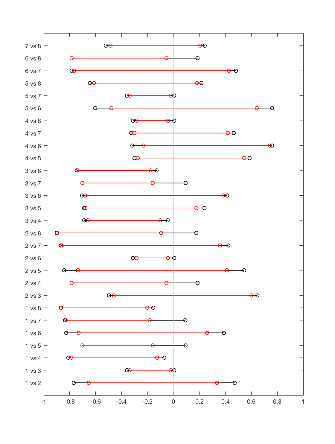
Figure 3: Sharp Bounds on Welfare Gaps under M1 (black) and M2 (red)

Figure 4: Sharp Partial Ordering under M2

As shown in Table 1, there are eight possible regimes, i.e., $\left|\mathcal{\mathcal{D}}\right|=\left|\mathcal{K}\right|=8$. We calculate the lower and upper bounds $(L_{k,k^{\prime}},U_{k,k^{\prime}})$ on the welfare gap $W_{k}-W_{k^{\prime}}$ for all pairs $k,k^{\prime}\in\{1,...,8\}$ ($k<k^{\prime}$). This is to illustrate the role of assumptions in improving the bounds. We conduct the bubble sort, which makes $\left(\begin{array}[]{c}8\\ 2\end{array}\right)$$=28$ pair-wise comparisons, resulting in $28\times 2$ linear programs to run. As the researcher, we maintain Assumption K. Then, for each linear program, the dimension of $q$ is $\left|\mathcal{Q}\right|+1=\left|\mathcal{S}\right|=\left|\mathcal{S}_{1}\right|\times\left|\mathcal{S}_{2}\right|=2^{2}\times 2^{2}\times 2^{8}\times 2^{4}=65,536$. The number of main constraints is $\dim(p)=2^{3\times 2}-2^{2}=60$. There are $1+65,536$ additional constraints that define the simplex, i.e., $\sum_{s}q_{s}=1$ and $q_{s}\geq 0$ for all $s\in\mathcal{S}$. Each linear program takes less than a second to calculate $L_{k,k^{\prime}}$ or $U_{k,k^{\prime}}$ with a computer with a 2.2 GHz single-core processor and 16 GB memory and with a modern solver such as CPLEX, MOSEK, and GUROBI.

Figure 3 reports the bounds $(L_{k,k^{\prime}},U_{k,k^{\prime}})$ on $W_{k}-W_{k^{\prime}}$ for all $(k,k^{\prime})\in\{1,...,8\}$ under Assumption M1 (in black) and Assumption M2 (in red). In the figure, we can determine the sign of the welfare gap for those bounds that exclude zero. The difference between the black and red bounds illustrates the role of Assumption M2 relative to M1. That is, there are more bounds that avoid the zero vertical line with M2, which is consistent with the theory. It is important to note that, because M2 does not assume the direction of monotonicity, the sign of the welfare gap is not imposed by the assumption but recovered from the data. Each set of bounds generates an associated partial ordering as a DAG (produced as an $8\times 8$ adjacency matrix). We proceed with Assumption M2 for brevity.

Figure 4 (identical to Figure 1 in the Introduction) depicts the sharp partial ordering generated from $(L_{k,k^{\prime}},U_{k,k^{\prime}})$’s under Assumption M2, based on Theorem 4.1(i). Then, by Theorem 4.1(ii), the identified set of $\boldsymbol{\delta}^{*}(\cdot)$ is

$$\mathcal{D}_{p}^{*} =\{\boldsymbol{\delta}_{7}(\cdot),\boldsymbol{\delta}_{8}(\cdot)\}.$$

The common feature of the elements in $\mathcal{D}_{p}^{*}$ is that it is optimal to allocate $\delta_{2}=1$ for all $y_{1}\in\{0,1\}$. Finally, the following is one of the topological sorts produced from the partial ordering:

$$(\boldsymbol{\delta}_{8}(\cdot),\boldsymbol{\delta}_{4}(\cdot),\boldsymbol{\delta}_{7}(\cdot),\boldsymbol{\delta}_{3}(\cdot),\boldsymbol{\delta}_{5}(\cdot),\boldsymbol{\delta}_{1}(\cdot),\boldsymbol{\delta}_{6}(\cdot),\boldsymbol{\delta}_{2}(\cdot)).$$

We also conducted a parallel analysis but with a slightly different data-generating process, where (a) all the coefficients in (8.1)–(8.4) are positive except $\mu_{22}<0$ and (b) $Z_{2}$ does not exist. In Case (a), we obtain $\mathcal{D}_{p}^{*}=\{\boldsymbol{\delta}_{2}(\cdot)\}$ as a singleton, i.e., we point identify $\boldsymbol{\delta}^{*}(\cdot)=\boldsymbol{\delta}_{2}(\cdot)$. The partial ordering for Case (b) is shown in Figure 5. In this case, we obtain $\mathcal{D}_{p}^{*}=\{\boldsymbol{\delta}_{6}(\cdot),\boldsymbol{\delta}_{7}(\cdot),\boldsymbol{\delta}_{8}(\cdot)\}$.

Figure 5: Sharp Partial Ordering under M2 (with only $Z_{1}$)

9 Application

We apply the framework of this paper to understand returns to schooling and post-school training as a sequence of treatments and to conduct a policy analysis. Schooling and post-school training are two major interventions that affect various labor market outcomes, such as earnings and employment status (Ashenfelter and Card (2010)). These treatments also have influences on health outcomes, either directly or through the labor market outcomes, and thus of interest for public health policies (Backlund et al. (1996), McDonough et al. (1997), Case et al. (2002)). We find that the Job Training Partnership Act (JTPA) is an appropriate setting for our analysis. The JTPA program is one of the largest publicly-funded training programs in the United States for economically disadvantaged individuals. Unfortunately, the JTPA only concerns post-school trainings, which have been the main focus in the literature (Bloom et al. (1997), Abadie et al. (2002), Kitagawa and Tetenov (2018)). In this paper, we combine the JTPA Title II data with those from other sources regarding high school education to create a data set that allows us to study the effects of a high school (HS) diploma (or its equivalents) and the subsidized job trainings as a sequence of treatments. We consider high school diplomas rather than college degrees because the former is more relevant for the disadvantaged population of Title II of the JTPA program.

We are interested in the dynamic treatment regime $\boldsymbol{\delta}(\cdot)=(\delta_{1},\delta_{2}(\cdot))$, where $\delta_{1}$ is a HS diploma and $\delta_{2}(y_{1})$ is the job training program given pre-program earning type $y_{1}$. The motivation of having $\delta_{2}$ as a function of $y_{1}$ comes from acknowledging the dynamic nature of how earnings are formed under education and training. The first-stage allocation $\delta_{1}$ will affect the pre-program earning. This response may contain information about unobserved characteristics of the individuals. Therefore, the allocation of $\delta_{2}$ can be informed by being adaptive to $y_{1}$. Then, the counterfactual earning type in the terminal stage given $\boldsymbol{\delta}(\cdot)$ can be expressed as $Y_{2}(\boldsymbol{\delta}(\cdot))=Y_{2}(\delta_{1},\delta_{2}(Y_{1}(\delta_{1})))$ where $Y_{1}(\delta_{1})$ is the counterfactual earning type in the first stage given $\delta_{1}$. We are interested in the optimal regime $\boldsymbol{\delta}^{*}$ that maximizes each of the following welfares: the average terminal earning $E[Y_{2}(\boldsymbol{\delta}(\cdot))]$ and the average lifetime earning $E[Y_{1}(\delta_{1})]+E[Y_{2}(\boldsymbol{\delta}(\cdot))]$.

For the purpose of our analysis, we combine the JTPA data with data from the US Census and the National Center for Education Statistics (NCES), from which we construct the following set of variables: $Y_{2}$ above or below median of 30-month earnings, $D_{2}$ the job training program, $Z_{2}$ a random assignment of the program, $Y_{1}$ above or below 80th percentile of pre-program earnings, $D_{1}$ the HS diploma or GED, and $Z_{1}$ the number of high schools per square mile. The instrument $Z_{1}$ for the HS treatment appears in the literature (e.g., Neal (1997)). The number of individuals in the sample is 9,223. We impose Assumptions SX and M2 throughout the analysis.

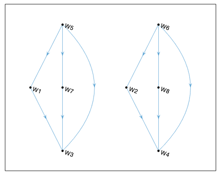
Regime #	$\delta_{1}$	$\delta_{2}(1,\delta_{1})$	$\delta_{2}(0,\delta_{1})$
1	0	0	0
2	1	0	0
3	0	1	0
4	1	1	0
5	0	0	1
6	1	0	1
7	0	1	1
8	1	1	1

Figure 6: Estimated Partial Ordering of $W_{\boldsymbol{\delta}}=E[Y_{2}(\boldsymbol{\delta}(\cdot))]$ and Estimated Set for $\boldsymbol{\delta}^{*}$ (red)

The estimation of the partial ordering (i.e., the DAG) and the identified set $\mathcal{D}_{p}^{*}$ is straightforward given the conditions in Theorem 4.1 and the linear programs (4.8). The only unknown object is $p$, the joint distribution of $(\boldsymbol{Y},\boldsymbol{D},\boldsymbol{Z})$, which can be estimated as $\hat{p}$, a vector of $\hat{p}_{\boldsymbol{y},\boldsymbol{d}|\boldsymbol{z}}=\sum_{i=1}^{N}1\{\boldsymbol{Y}_{i}=\boldsymbol{y},\boldsymbol{D}_{i}=\boldsymbol{d},\boldsymbol{Z}_{i}=\boldsymbol{z}\}/\sum_{i=1}^{N}1\{\boldsymbol{Z}_{i}=\boldsymbol{z}\}$.

Figure 6 reports the estimated partial ordering of welfare $W_{\boldsymbol{\delta}}=E[Y_{2}(\boldsymbol{\delta}(\cdot))]$ (left) and the resulting estimated set $\hat{\mathcal{D}}$ (right, highlighted in red) that we estimate using $\{(\boldsymbol{Y}_{i},\boldsymbol{D}_{i},\boldsymbol{Z}_{i})\}_{i=1}^{9,223}$. Although there exist welfares that cannot be ordered, we can conclude with certainty that allocating the program only to the low earning type ($Y_{2}=0$) is welfare optimal, as it is the common implication of Regimes 5 and 6 in $\hat{\mathcal{D}}$. Also, the second best policy is to either allocate the program to the entire population or none, while allocating it only to the high earning type ($Y_{2}=1$) produces the lowest welfare. This result is consistent with the eligibility of Title II of the JTPA, which concerns individuals with “barriers to employment” where the most common barriers are unemployment spells and high-school dropout status (Abadie et al. (2002)). Possibly due to the fact that the first-stage instrument $Z_{1}$ is not strong enough, we have the two disconnected sub-DAGs and thus the two elements in $\hat{\mathcal{D}}$, which are agnostic about the optimal allocation in the first stage or the complementarity between the first- and second- stage allocations.

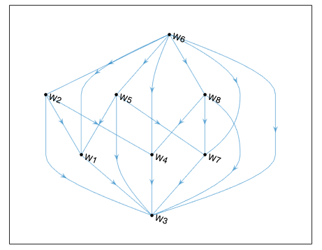
Regime #	$\delta_{1}$	$\delta_{2}(1,\delta_{1})$	$\delta_{2}(0,\delta_{1})$
1	0	0	0
2	1	0	0
3	0	1	0
4	1	1	0
5	0	0	1
6	1	0	1
7	0	1	1
8	1	1	1

Figure 7: Estimated Partial Ordering of $W_{\boldsymbol{\delta}}=E[Y_{1}(\delta_{1})]+E[Y_{2}(\boldsymbol{\delta}(\cdot))]$ and Estimated Set for $\boldsymbol{\delta}^{*}$ (red)

Figure 7 reports the estimated partial ordering and the estimated set with $W_{\boldsymbol{\delta}}=E[Y_{1}(\delta_{1})]+E[Y_{2}(\boldsymbol{\delta}(\cdot))]$. Despite the partial ordering, $\hat{\mathcal{D}}$ is a singleton for this welfare and $\boldsymbol{\delta}^{*}$ is estimated to be Regime 6. According to this regime, the average lifetime earning is maximized by allocating HS education to all individuals and the training program to individuals with low pre-program earnings. As discussed earlier, additional policy implications can be obtained by inspecting suboptimal regimes. Interestingly, Regime 8, which allocates the treatments regardless, is inferior to Regime 6. This can be useful knowledge for policy makers especially because Regime 8 is the most “expensive” regime. Similarly, Regime 1, which does not allocate any treatments regardless and thus is the least expensive regime, is superior to Regime 3, which allocates the program to high-earning individuals. The estimated partial ordering shows how more expensive policies do not necessarily achieve greater welfare. Moreover, these conclusions can be compelling as they are drawn without making arbitrary parametric restrictions nor strong identifying assumptions.

Finally, as an alternative approach, we use $\{(\boldsymbol{Y}_{i},\boldsymbol{D}_{i},Z_{2i})\}_{i=1}^{9,223}$ for estimation, that is, we drop $Z_{1}$ and only use the exogenous variation from $Z_{2}$. This reflects a possible concern that $Z_{1}$ may not be as valid as $Z_{2}$. Then, the estimated partial ordering looks identical to the left panel of Figure 6 whether the targeted welfare is $E[Y_{2}(\boldsymbol{\delta}(\cdot))]$ or $E[Y_{1}(\delta_{1})]+E[Y_{2}(\boldsymbol{\delta}(\cdot))]$. Clearly, without $Z_{1}$, the procedure lacks the ability to determine the first stage’s best treatment. Note that, even though the partial ordering for $E[Y_{2}(\boldsymbol{\delta}(\cdot))]$ is identical for the case of one versus two instruments, the inference results will reflect such difference by producing a larger confidence set for the former case.

10 Inference

Although we do not fully investigate inference in the current paper, we briefly discuss it. To conduct inference on the optimal regime $\boldsymbol{\delta}^{*}(\cdot)$, we can construct a confidence set (CS) for $\mathcal{D}_{p}^{*}$ with the following procedure. We consider a sequence of hypothesis tests, in which we eliminate regimes that are (statistically) significantly inferior to others. This is a statistical analog of the elimination procedure encoded in (4.9) or (4.10). For each test given $\tilde{\mathcal{K}}\subset\mathcal{K}$, we construct a null hypothesis that $W_{k}$ and $W_{k^{\prime}}$ are not comparable for all $k,k^{\prime}\in\tilde{\mathcal{K}}$. Given (4.8), the incomparability of $W_{k}$ and $W_{k^{\prime}}$ is equivalent to $L_{k,k^{\prime}}\leq 0\leq U_{k,k^{\prime}}$. In constructing the null hypothesis, it is helpful to invoke strong duality for the primal programs (4.8) and write the following dual programs:

$$U_{k,k^{\prime}}= \min_{\lambda}\tilde{p}^{\prime}\lambda,\qquad s.t.\quad\tilde{B}^{\prime}\lambda\geq\Delta_{k,k^{\prime}}^{\prime}$$ (10.1)

$$L_{k,k^{\prime}}= \max_{\lambda}-\tilde{p}^{\prime}\lambda,\qquad s.t.\quad\tilde{B}^{\prime}\lambda\geq-\Delta_{k,k^{\prime}}^{\prime}$$ (10.2)

where $\tilde{B}\equiv\left[\begin{array}[]{c}B\\ \boldsymbol{1}^{\prime}\end{array}\right]$ is a $(d_{p}+1)\times d_{q}$ matrix with $\boldsymbol{1}$ being a $d_{q}\times 1$ vector of ones and $\tilde{p}\equiv\left[\begin{array}[]{c}p\\ 1\end{array}\right]$ is a $(d_{p}+1)\times 1$ vector. By using a vertex enumeration algorithm (e.g., Avis and Fukuda (1992)), one can find all (or a relevant subset) of vertices of the polyhedra $\{\lambda:\tilde{B}^{\prime}\lambda\geq\Delta_{k,k^{\prime}}^{\prime}\}$ and $\{\lambda:\tilde{B}^{\prime}\lambda\geq-\Delta_{k,k^{\prime}}^{\prime}\}$. Let $\Lambda_{U,k,k^{\prime}}\equiv\{\lambda_{1},...,\lambda_{J_{U,k,k^{\prime}}}\}$ and $\Lambda_{L,k,k^{\prime}}\equiv\{\lambda_{1},...,\lambda_{J_{L,k,k^{\prime}}}\}$ be the sets that collect such vertices, respectively. Then, it is easy to see that $U_{k,k^{\prime}}=\min_{\lambda\in\Lambda_{U,k,k^{\prime}}}\tilde{p}^{\prime}\lambda$ and $L_{k,k^{\prime}}=\max_{\lambda\in\Lambda_{L,k,k^{\prime}}}-\tilde{p}^{\prime}\lambda$. Therefore, the null hypothesis that $L_{k,k^{\prime}}\leq 0\leq U_{k,k^{\prime}}$ can be written as

$$H_{0,\tilde{\mathcal{K}}} :\tilde{p}^{\prime}\lambda>0\text{ for all }\lambda\in\Lambda_{\tilde{\mathcal{K}}}.$$ (10.3)

where $\Lambda_{\tilde{\mathcal{K}}}\equiv\bigcup_{k,k^{\prime}\in\tilde{\mathcal{K}}}\Lambda_{k,k^{\prime}}$ with $\Lambda_{k,k^{\prime}}\equiv\Lambda_{U,k,k^{\prime}}\cup\Lambda_{L,k,k^{\prime}}$.

Then, the procedure of constructing the CS, denoted as $\widehat{\mathcal{D}}_{CS}$, is as follows: Step 0. Initially set $\tilde{\mathcal{K}}=\mathcal{K}$. Step 1. Test $H_{0,\tilde{\mathcal{K}}}$ at level $\alpha$ with test function $\phi_{\tilde{\mathcal{K}}}\in\{0,1\}$. Step 2. If $H_{0,\tilde{\mathcal{K}}}$ is not rejected, define $\widehat{\mathcal{D}}_{CS}=\{\boldsymbol{\delta}_{k}(\cdot):k\in\tilde{\mathcal{K}}\}$; otherwise eliminate vertex $k_{\tilde{\mathcal{K}}}$ from $\tilde{\mathcal{K}}$ and repeat from Step 1. In Step 1, $T_{\tilde{\mathcal{K}}}\equiv\min_{k,k^{\prime}\in\tilde{\mathcal{K}}}t_{k,k^{\prime}}$ can be used as the test statistic for $H_{0,\tilde{\mathcal{K}}}$ where $t_{k,k^{\prime}}\equiv\min_{\lambda\in\Lambda_{k,k^{\prime}}}t_{\lambda}$ and $t_{\lambda}$ is a standard $t$-statistic. The distribution of $T_{\tilde{\mathcal{K}}}$ can be estimated using bootstrap. In Step 2, a candidate for $k_{\tilde{\mathcal{K}}}$ is $k_{\tilde{\mathcal{K}}}\equiv\arg\min_{k\in\tilde{\mathcal{K}}}\min_{k^{\prime}\in\tilde{\mathcal{K}}}t_{k,k^{\prime}}$.

The eliminated vertices (i.e., regimes) are statistically suboptimal regimes, which are already policy-relevant outputs of the procedure. Note that the null hypothesis (10.3) consists of multiple inequalities. This incurs the issue of uniformity in that the null distribution depends on binding inequalities, whose identities are unknown. Such a problem has been studied in the literature, as in Hansen (2005), Andrews and Soares (2010), and Chen and Szroeter (2014). Hansen et al. (2011)’s bootstrap approach for constructing the model confidence set builds on Hansen (2005). We apply a similar inference method as in Hansen et al. (2011), but in this novel context and by being conscious about the computational challenge of our problem. In particular, the dual problem (10.1)–(10.2) and the vertex enumeration algorithm are introduced to ease the computational burden in simulating the distribution of $T_{\tilde{\mathcal{K}}}$. That is, the calculation of $\Lambda_{\tilde{\mathcal{K}}}$, the computationally intensive step, occurs only once, and then for each bootstrap sample, it suffices to calculate $\hat{p}$ instead of solving the linear programs (4.8) for all $k,k^{\prime}\in\tilde{\mathcal{K}}$.

Analogous to Hansen et al. (2011), we can show that the resulting CS has desirable properties. Let $H_{A,\tilde{\mathcal{K}}}$ be the alternative hypothesis.

Assumption CS.

For any $\tilde{\mathcal{K}}$, (i) $\limsup_{n\rightarrow\infty}\Pr[\phi_{\tilde{\mathcal{K}}}=1|H_{0,\tilde{\mathcal{K}}}]\leq\alpha$, (ii) $\lim_{n\rightarrow\infty}\Pr[\phi_{\tilde{\mathcal{K}}}=1|H_{A,\tilde{\mathcal{K}}}]=1$, and (iii) $\lim_{n\rightarrow\infty}\Pr[\boldsymbol{\delta}_{k_{\tilde{\mathcal{K}}}}(\cdot)\in\mathcal{\mathcal{D}}_{p}^{*}|H_{A,\tilde{\mathcal{K}}}]=0$.

Proposition 10.1.

Under Assumption CS, it satisfies that $\lim\inf_{n\rightarrow\infty}\Pr[\mathcal{D}_{p}^{*}\subset\widehat{\mathcal{D}}_{CS}]\geq 1-\alpha$ and $\lim_{n\rightarrow\infty}\Pr[\boldsymbol{\delta}(\cdot)\in\widehat{\mathcal{D}}_{CS}]=0$ for all $\boldsymbol{\delta}(\cdot)\notin\mathcal{\mathcal{D}}_{p}^{*}$.

The procedure of constructing the CS does not suffer from the problem of multiple testings. This is because the procedure stops as soon as the first hypothesis is not rejected, and asymptotically, maximal elements will not be questioned before all sub-optimal regimes are eliminated. The resulting CS can also be used to conduct a specification test for a less palatable assumption, such as Assumption M2. We can refute the assumption when the CS under that assumption is empty.

Inference on the welfare bounds in (5.4) for a given regime can be conducted by using recent results as in Deb et al. (2017), who develop uniformly valid inference that can be applied to bounds obtained via linear programming. Inference on optimized welfare $W_{\boldsymbol{\delta}^{*}}$ or $\max_{\boldsymbol{\delta}(\cdot)\in\widehat{\mathcal{D}}_{CS}}W_{\boldsymbol{\delta}}$ can also be an interesting problem. Andrews et al. (2019) consider inference on optimized welfare (evaluated at the estimated policy) in the context of Kitagawa and Tetenov (2018), but with point-identified welfare under the unconfoundedness assumption. Extending the framework to the current setting with partially identified welfare and dynamic regimes under treatment endogeneity would also be interesting future work.

Appendix A Appendix

A.1 Stochastic Regimes

For each $t=1,...,T$, define an adaptive stochastic treatment rule $\tilde{\delta}_{t}:\{0,1\}^{t-1}\times\{0,1\}^{t-1}\rightarrow[0,1]$ that allocates the probability of treatment:

$$\tilde{\delta}_{t}(\boldsymbol{y}^{t-1},\tilde{\boldsymbol{d}}^{t-1}) =\tilde{d}_{t}\in[0,1].$$ (A.1)

Then, the vector of these $\tilde{\delta}_{t}$’s is a dynamic stochastic regime $\tilde{\boldsymbol{\delta}}(\cdot)\equiv\tilde{\boldsymbol{\delta}}^{T}(\cdot)\in\mathcal{D}_{stoch}$ where $\mathcal{D}_{stoch}$ is the set of all possible stochastic regimes. A deterministic regime is a special case where $\tilde{\delta}_{t}(\cdot)$ takes the extreme values of $1$ and $0$. Therefore, $\mathcal{D}\subset\mathcal{D}_{stoch}$ where $\mathcal{D}$ is the set of deterministic regimes. We define $Y_{T}(\tilde{\boldsymbol{\delta}}(\cdot))$ with $\tilde{\boldsymbol{\delta}}(\cdot)\in\mathcal{D}_{stoch}$ as the counterfactual outcome $Y_{T}(\boldsymbol{\delta}(\cdot))$ where the deterministic rule $\delta_{t}(\cdot)=1$ is randomly assigned with probability $\tilde{\delta}_{t}(\cdot)$ and $\delta_{t}(\cdot)=0$ otherwise for all $t\leq T$. Finally, define

$$W_{\tilde{\boldsymbol{\delta}}} \equiv\mathbb{E}[Y_{T}(\tilde{\boldsymbol{\delta}}(\cdot))],$$

where $\mathbb{E}$ denotes an expectation over the counterfactual outcome and the random mechanism defining a rule, and define $\tilde{\boldsymbol{\delta}}^{*}(\cdot)\equiv\arg\max_{\tilde{\boldsymbol{\delta}}(\cdot)\in\mathcal{D}_{stoch}}W_{\tilde{\boldsymbol{\delta}}}$. The following theorem show that a deterministic regime is achieved as being optimal even though stochastic regimes are allow.

Theorem A.1.

Suppose $W_{\tilde{\boldsymbol{\delta}}}\equiv\mathbb{E}[Y_{T}(\tilde{\boldsymbol{\delta}}(\cdot))]$ for $\tilde{\boldsymbol{\delta}}(\cdot)\in\mathcal{D}_{stoch}$ and $W_{\boldsymbol{\delta}}\equiv E[Y_{T}(\boldsymbol{\delta}(\cdot))]$ for $\boldsymbol{\delta}(\cdot)\in\mathcal{D}$. It satisfies that

$$\boldsymbol{\delta}^{*}(\cdot)\equiv\arg\max_{\boldsymbol{\delta}(\cdot)\in\mathcal{D}}W_{\boldsymbol{\delta}} =\arg\max_{\tilde{\boldsymbol{\delta}}(\cdot)\in\mathcal{D}_{stoch}}W_{\tilde{\boldsymbol{\delta}}}.$$

By the law of iterative expectation, we have

$$\mathbb{E}[Y_{T}(\tilde{\boldsymbol{\delta}}(\cdot))] =\mathbb{E}\left[\mathbb{E}\left[\left.\cdots\mathbb{E}\left[\left.\mathbb{E}[Y_{T}(\tilde{\boldsymbol{d}})|\boldsymbol{Y}^{T-1}(\tilde{\boldsymbol{d}}^{T-1})]\right|\boldsymbol{Y}^{T-2}(\tilde{\boldsymbol{d}}^{T-2})\right]\cdots\right|Y_{1}(\tilde{d}_{1})\right]\right],$$ (A.2)

where the bridge variables $\tilde{\boldsymbol{d}}=(\tilde{d}_{1},...,\tilde{d}_{T})$ satisfy

$$\tilde{d}_{1} =\tilde{\delta}_{1},$$

$$\tilde{d}_{2} =\tilde{\delta}_{2}(Y_{1}(\tilde{d}_{1}),\tilde{d}_{1}),$$

$$\tilde{d}_{3} =\tilde{\delta}_{3}(\boldsymbol{Y}^{2}(\tilde{\boldsymbol{d}}^{2}),\tilde{\boldsymbol{d}}^{2}),$$

$$\vdots$$

$$\tilde{d}_{T} =\tilde{\delta}_{T}(\boldsymbol{Y}^{T-1}(\tilde{\boldsymbol{d}}^{T-1}),\tilde{\boldsymbol{d}}^{T-1}).$$

Given (A.2), we prove the theorem by showing that the solution $\tilde{\boldsymbol{\delta}}^{*}(\cdot)$ can be justified by backward induction in a finite-horizon dynamic programming. To illustrate this with deterministic regimes when $T=2$, we have

$$\delta_{2}^{*}(y_{1},d_{1}) =\arg\max_{d_{2}}E[Y_{2}(\boldsymbol{d})|Y_{1}(d_{1})=y_{1}],$$ (A.3)

and, by defining $V_{2}(y_{1},d_{1})\equiv\max_{d_{2}}E[Y_{2}(\boldsymbol{d})|Y_{1}(d_{1})=y_{1}]$,

$$\delta_{1}^{*}= \arg\max_{d_{1}}E[V_{2}(Y_{1}(d_{1}),d_{1})].$$ (A.4)

Then, $\boldsymbol{\delta}^{*}(\cdot)$ is equal to the collection of these solutions: $\boldsymbol{\delta}^{*}(\cdot)=(\delta_{1}^{*},\delta_{2}^{*}(\cdot))$.

Proof.

First, given (A.2), the optimal stochastic rule in the final period can be defined as

$$\tilde{\delta}_{T}^{*}(\boldsymbol{y}^{T-1},\tilde{\boldsymbol{d}}^{T-1})\equiv \arg\max_{\tilde{d}_{T}\in[0,1]}\mathbb{E}[Y_{T}(\tilde{\boldsymbol{d}})|\boldsymbol{Y}^{T-1}(\tilde{\boldsymbol{d}}^{T-1})=\boldsymbol{y}^{T-1}].$$

Define a value function at period $T$ as $V_{T}(\boldsymbol{y}^{T-1},\tilde{\boldsymbol{d}}^{T-1})\equiv\max_{\tilde{d}_{T}}\mathbb{E}[Y_{T}(\tilde{\boldsymbol{d}})|\boldsymbol{Y}^{T-1}(\tilde{\boldsymbol{d}}^{T-1})=\boldsymbol{y}^{T-1}]$. Similarly, for each $t=1,...,T-1$, let

$$\tilde{\delta}_{t}^{*}(\boldsymbol{y}^{t-1},\tilde{\boldsymbol{d}}^{t-1})\equiv \arg\max_{\tilde{d}_{t}\in[0,1]}\mathbb{E}[V_{t+1}(\boldsymbol{Y}^{t}(\tilde{\boldsymbol{d}}^{t}),\tilde{\boldsymbol{d}}^{t})|\boldsymbol{Y}^{t-1}(\tilde{\boldsymbol{d}}^{t-1})=\boldsymbol{y}^{t-1}]$$

and $V_{t}(\boldsymbol{y}^{t-1},\tilde{\boldsymbol{d}}^{t-1})\equiv\max_{\tilde{d}_{t}}\mathbb{E}[V_{t+1}(\boldsymbol{Y}^{t}(\tilde{\boldsymbol{d}}^{t}),\tilde{\boldsymbol{d}}^{t})|\boldsymbol{Y}^{t-1}(\tilde{\boldsymbol{d}}^{t-1})=\boldsymbol{y}^{t-1}]$. Then, $\tilde{\boldsymbol{\delta}}^{*}(\cdot)=(\tilde{\delta}_{1}^{*},...,\tilde{\delta}_{T}^{*}(\cdot))$. Since $\{0,1\}\subset[0,1]$, the same argument can apply for the deterministic regime using the current framework but each maximization domain being $\{0,1\}$. This analogously defines $\delta_{t}^{*}(\cdot)\in\{0,1\}$ for all $t$, and then $\boldsymbol{\delta}^{*}(\cdot)=(\delta_{1}^{*},...,\delta_{T}^{*}(\cdot))$, similarly as in Murphy (2003).

Now, for the maximization problems above, let $\tilde{W}_{t}(\tilde{\boldsymbol{d}}^{t},\boldsymbol{y}^{t-1})$ represent the objective function at $t$ for $2\leq t\leq T$ with $\tilde{W}_{1}(\tilde{d}_{1})$ for $t=1$. By the definition of the stochastic regime, it satisfies that

$$\tilde{W}_{t}(\tilde{\boldsymbol{d}}^{t},\boldsymbol{y}^{t-1}) =\tilde{d}_{t}W_{t}(1,\tilde{\boldsymbol{d}}^{t-1},\boldsymbol{y}^{t-1})+(1-\tilde{d}_{t})W_{t}(0,\tilde{\boldsymbol{d}}^{t-1},\boldsymbol{y}^{t-1})$$

$$=\tilde{d}_{t}\left\{W_{t}(1,\tilde{\boldsymbol{d}}^{t-1},\boldsymbol{y}^{t-1})-W_{t}(0,\tilde{\boldsymbol{d}}^{t-1},\boldsymbol{y}^{t-1})\right\}+W_{t}(0,\tilde{\boldsymbol{d}}^{t-1},\boldsymbol{y}^{t-1}).$$

Therefore, $W_{t}(1,\tilde{\boldsymbol{d}}^{t-1},\boldsymbol{y}^{t-1})\geq W_{t}(0,\tilde{\boldsymbol{d}}^{t-1},\boldsymbol{y}^{t-1})$ or $1=\arg\max_{\tilde{d}_{t}\in\{0,1\}}\tilde{W}_{t}(\tilde{\boldsymbol{d}}^{t},\boldsymbol{y}^{t-1})$ if and only if $1=\arg\max_{\tilde{d}_{t}\in[0,1]}\tilde{W}_{t}(\tilde{\boldsymbol{d}}^{t},\boldsymbol{y}^{t-1})$. Symmetrically, $0=\arg\max_{\tilde{d}_{t}\in\{0,1\}}\tilde{W}_{t}(\tilde{\boldsymbol{d}}^{t},\boldsymbol{y}^{t-1})$ if and only if $0=\arg\max_{\tilde{d}_{t}\in[0,1]}\tilde{W}_{t}(\tilde{\boldsymbol{d}}^{t},\boldsymbol{y}^{t-1})$. This implies that $\tilde{\delta}_{t}^{*}(\cdot)=\delta_{t}^{*}(\cdot)$ for all $t=1,...,T$, which proves the theorem.∎

A.2 Matrices in Section 4.3

We show how to construct matrices $A_{k}$ and $B$ in (4.2) and (4.4) for the linear programming (4.8). The construction of $A_{k}$ and $B$ uses the fact that any linear functional of $\Pr[\boldsymbol{Y}(\boldsymbol{d})=\boldsymbol{y},\boldsymbol{D}(\boldsymbol{z})=\boldsymbol{d}]$ can be characterized as a linear combination of $q_{s}$. Although the notation of this section can be somewhat heavy, if one is committed to the use of linear programming instead of an analytic solution, most of the derivation can be systematically reproduced in a standard software, such as MATLAB and Python.

Consider $B$ first. By Assumption SX, we have

$$p_{\boldsymbol{y},\boldsymbol{d}|\boldsymbol{z}} =\Pr[\boldsymbol{Y}(\boldsymbol{d})=\boldsymbol{y},\boldsymbol{D}(\boldsymbol{z})=\boldsymbol{d}]$$

$$=\Pr[\boldsymbol{Y}(\boldsymbol{y}^{T-1},\boldsymbol{d})=\boldsymbol{y},\boldsymbol{D}(\boldsymbol{y}^{T-1},\boldsymbol{d}^{T-1},\boldsymbol{z})=\boldsymbol{d}]$$

$$=\Pr[S:Y_{t}(\boldsymbol{y}^{t-1},\boldsymbol{d}^{t})=y_{t},D_{t}(\boldsymbol{y}^{t-1},\boldsymbol{d}^{t-1},\boldsymbol{z}^{t})=d_{t}\quad\forall t]$$

$$=\sum_{s\in\mathcal{S}_{\boldsymbol{y},\boldsymbol{d}|\boldsymbol{z}}}q_{s},$$ (A.5)

where $\mathcal{S}_{\boldsymbol{y},\boldsymbol{d}|\boldsymbol{z}}\equiv\{S=\beta(\tilde{\boldsymbol{S}}):Y_{t}(\boldsymbol{y}^{t-1},\boldsymbol{d}^{t})=y_{t},D_{t}(\boldsymbol{y}^{t-1},\boldsymbol{d}^{t-1},\boldsymbol{z}^{t})=d_{t}\text{ }\forall t\}$, $\tilde{\boldsymbol{S}}\equiv(\tilde{S}_{1},...,\tilde{S}_{T})$ with $\tilde{S}_{t}\equiv(\{Y_{t}(\boldsymbol{y}^{t-1},\boldsymbol{d}^{t})\},\{D_{t}(\boldsymbol{y}^{t-1},\boldsymbol{d}^{t-1},\boldsymbol{z}^{t})\})$, and $\beta(\cdot)$ is a one-to-one map that transforms a binary sequence into a decimal value. Then, for a $1\times d_{q}$ vector $B_{\boldsymbol{y},\boldsymbol{d}|\boldsymbol{z}}$,

$$p_{\boldsymbol{y},\boldsymbol{d}|\boldsymbol{z}} =\sum_{s\in\mathcal{S}_{\boldsymbol{y},\boldsymbol{d}|\boldsymbol{z}}}q_{s}=B_{\boldsymbol{y},\boldsymbol{d}|\boldsymbol{z}}q$$

and the $d_{p}\times d_{q}$ matrix $B$ stacks $B_{\boldsymbol{y},\boldsymbol{d}|\boldsymbol{z}}$ so that $p=Bq$.

For $A_{k}$, recall $W_{\boldsymbol{\delta}_{k}}$ is a linear functional of $q_{\boldsymbol{\delta}_{k}}(\boldsymbol{y})\equiv\Pr[\boldsymbol{Y}(\boldsymbol{\delta}_{k}(\cdot))=\boldsymbol{y}]$. For given $\boldsymbol{\delta}(\cdot)$, by repetitively applying the law of iterated expectation, we can show

$$\Pr[\boldsymbol{Y}(\boldsymbol{\delta}(\cdot))=\boldsymbol{y}]$$

$$= \Pr[Y_{T}(\boldsymbol{d})=y_{T}|\boldsymbol{Y}^{T-1}(\boldsymbol{d}^{T-1})=\boldsymbol{y}^{T-1}]$$

$$\times\Pr[Y_{T-1}(\boldsymbol{d}^{T-1})=y_{T-1}|\boldsymbol{Y}^{T-2}(\boldsymbol{d}^{T-2})=\boldsymbol{y}^{T-2}]\times\cdots\times\Pr[Y_{1}(d_{1})=y_{1}],$$ (A.6)

where, because of the appropriate conditioning in (A.6), the bridge variables $\boldsymbol{d}=(d_{1},...,d_{T})$ satisfies

$$d_{1} =\delta_{1},$$

$$d_{2} =\delta_{2}(y_{1},d_{1}),$$

$$d_{3} =\delta_{3}(\boldsymbol{y}^{2},\boldsymbol{d}^{2}),$$

$$\vdots$$

$$d_{T} =\delta_{T}(\boldsymbol{y}^{T-1},\boldsymbol{d}^{T-1}).$$

Therefore, (A.6) can be viewed as a linear functional of $\Pr[\boldsymbol{Y}(\boldsymbol{d})=\boldsymbol{y}]$. To illustrate, when $T=2$, the welfare defined as the average counterfactual terminal outcome satisfies

$$E[Y_{T}(\boldsymbol{\delta}(\cdot))] =\sum_{y_{1}}\Pr[Y_{2}(\delta_{1},\delta_{2}(Y_{1}(\delta_{1}),\delta_{1}))=1|Y_{1}(\delta_{1})=y_{1}]\Pr[Y_{1}(\delta_{1})=y_{1}]$$

$$=\sum_{y_{1}}\Pr[Y_{2}(\delta_{1},\delta_{2}(y_{1},\delta_{1}))=1,Y_{1}(\delta_{1})=y_{1}].$$ (A.7)

Then, for a chosen $\boldsymbol{\delta}(\cdot)$, the values $\delta_{1}=d_{1}$ and $\delta_{2}(y_{1},\delta_{1})=d_{2}$ at which $Y_{2}(\delta_{1},\delta_{2}(y_{1},\delta_{1}))$ and $Y_{1}(\delta_{1})$ are defined is given in Table 1 as shown in the main text. Therefore, $E[Y_{2}(\boldsymbol{\delta}(\cdot))]$ can be written as a linear functional of $\Pr[Y_{2}(d_{1},d_{2})=y_{2},Y_{1}(d_{1})=y_{1}]$.

Now, define a linear functional $h_{k}(\cdot)$ that (i) marginalizes $\Pr[\boldsymbol{Y}(\boldsymbol{d})=\boldsymbol{y},\boldsymbol{D}(\boldsymbol{z})=\boldsymbol{d}]$ into $\Pr[\boldsymbol{Y}(\boldsymbol{d})=\boldsymbol{y}]$ and then (ii) maps $\Pr[\boldsymbol{Y}(\boldsymbol{d})=\boldsymbol{y}]$ into $\Pr[\boldsymbol{Y}(\boldsymbol{\delta}_{k}(\cdot))=\boldsymbol{y}]$ according to (A.6). But recall that $\Pr[\boldsymbol{Y}(\boldsymbol{d})=\boldsymbol{y},\boldsymbol{D}(\boldsymbol{z})=\boldsymbol{d}]=\sum_{s\in\mathcal{S}_{\boldsymbol{y},\boldsymbol{d}|\boldsymbol{z}}}q_{s}$ by (A.5). Consequently, we have

$$W_{k} =f(q_{\boldsymbol{\delta}_{k}})=f(\Pr[\boldsymbol{Y}(\boldsymbol{\delta}_{k}(\cdot))=\cdot])$$

$$=f\circ h_{k}(\Pr[\boldsymbol{Y}(\cdot)=\cdot,\boldsymbol{D}(\boldsymbol{z})=\cdot]),$$

$$=f\circ h_{k}\left(\sum_{s\in\mathcal{S}_{\cdot,\cdot|\boldsymbol{z}}}q_{s}\right)\equiv A_{k}q.$$

To continue the illustration (4.3) in the main text, note that

$$\Pr[\boldsymbol{Y}(1,1)=(1,1)]=\Pr[S:Y_{1}(1)=1,Y_{2}(1,1)=1]=\sum_{s\in\mathcal{S}_{11}}q_{s},$$

where $\mathcal{S}_{11}\equiv\{S=\beta(\tilde{S}_{1},\tilde{S}_{2}):Y_{1}(1)=1,Y_{2}(1,1)=1\}$. Similarly, we have

$$\Pr[\boldsymbol{Y}(1,1)=(0,1)]=\Pr[S:Y_{1}(1)=0,Y_{2}(1,1)=1]=\sum_{s\in\mathcal{S}_{01}}q_{s},$$

where $\mathcal{S}_{01}\equiv\{S=\beta(\tilde{S}_{1},\tilde{S}_{2}):Y_{1}(1)=0,Y_{2}(1,1)=1\}$.

A.3 Proof of Theorem 4.1

Let $\mathcal{Q}_{p}\equiv\{q:Bq=p\}\cap\mathcal{Q}$ be the feasible set. To prove part (i), first note that the sharp DAG can be explicitly defined as $G(\mathcal{K},\mathcal{E}_{p})$ with

$$\mathcal{E}_{p} \equiv\{(k,k^{\prime})\in\mathcal{K}:A_{k}q>A_{k^{\prime}}q\text{ for all }q\in\mathcal{Q}_{p}\}.$$

Here, $A_{k}q>A_{k^{\prime}}q$ for all $q\in\mathcal{Q}_{p}$ if and only if $L_{k,k^{\prime}}>0$ as $L_{k,k^{\prime}}$ is the sharp lower bound of $(A_{k}-A_{k^{\prime}})q$ in (4.8). The latter is because the feasible set $\{q:Bq=p\text{ and }q\in\mathcal{Q}\}$ is convex and thus $\{\Delta_{k,k^{\prime}}q:Bq=p\text{ and }q\in\mathcal{Q}\}$ is convex, which implies that any point between $[L_{k,k^{\prime}},U_{k,k^{\prime}}]$ is attainable.

To prove part (ii), it is helpful to note that $\mathcal{D}_{p}^{*}$ in (4.5) can be equivalently defined as

$$\mathcal{D}_{p}^{*} \equiv\{\boldsymbol{\delta}_{k^{\prime}}(\cdot):\nexists k\in\mathcal{K}\text{ such that }A_{k}q>A_{k^{\prime}}q\text{ for all }q\in\mathcal{Q}_{p}\}$$

$$=\{\boldsymbol{\delta}_{k^{\prime}}(\cdot):A_{k}q\leq A_{k^{\prime}}q\text{ for all }k\in\mathcal{K}\text{ and some }q\in\mathcal{Q}_{p}\}.$$

Let $\tilde{\mathcal{D}}_{p}^{*}\equiv\{\boldsymbol{\delta}_{k^{\prime}}(\cdot):\nexists k\in\mathcal{K}\text{ such that }L_{k,k^{\prime}}>0\text{ and }k\neq k^{\prime}\}$. First, we prove that $\mathcal{D}_{p}^{*}\subset\tilde{\mathcal{D}}_{p}^{*}$. Note that

$$\mathcal{D}\backslash\tilde{\mathcal{D}}_{p}^{*} =\{\boldsymbol{\delta}_{k^{\prime}}:L_{k,k^{\prime}}>0\text{ for some }k\neq k^{\prime}\}.$$

Suppose $\boldsymbol{\delta}_{k^{\prime}}\in\mathcal{D}\backslash\tilde{\mathcal{D}}_{p}^{*}$. Then, for some $k\neq k^{\prime}$, $(A_{k}-A_{k^{\prime}})q\geq L_{k,k^{\prime}}>0$ for all $q\in\mathcal{Q}_{p}$. Therefore, for such $k$, $A_{k}q>A_{k^{\prime}}q$ for all $q\in\mathcal{Q}_{p}$, and thus $\boldsymbol{\delta}_{k^{\prime}}\notin\mathcal{D}_{p}^{*}\equiv\{\arg\max_{\boldsymbol{\delta}_{k}}A_{k}q:q\in\mathcal{Q}_{p}\}$.

Now, we prove that $\tilde{\mathcal{D}}_{p}^{*}\subset\mathcal{D}_{p}^{*}$. Suppose $\boldsymbol{\delta}_{k^{\prime}}\in\tilde{\mathcal{D}}_{p}^{*}$. Then $\nexists k\neq k^{\prime}$ such that $L_{k,k^{\prime}}>0$. Equivalently, for any given $k\neq k^{\prime}$, either (a) $U_{k,k^{\prime}}\leq 0$ or (b) $L_{k,k^{\prime}}<0<U_{k,k^{\prime}}$. Consider (a), which is equivalent to $\max_{q\in\mathcal{Q}_{p}}(A_{k}-A_{k^{\prime}})q\leq 0$. This implies that $A_{k}q\leq A_{k^{\prime}}q$ for all $q\in\mathcal{Q}_{p}$. Consider (b), which is equivalent to $\min_{q\in\mathcal{Q}_{p}}(A_{k}-A_{k^{\prime}})q<0<\max_{q\in\mathcal{Q}_{p}}(A_{k}-A_{k^{\prime}})q$. This implies that $\exists q\in\mathcal{Q}_{p}$ such that $A_{k}q=A_{k^{\prime}}q$. Combining these implications of (a) and (b), it should be the case that $\exists q\in\mathcal{Q}_{p}$ such that, for all $k\neq k^{\prime}$, $A_{k^{\prime}}q\geq A_{k}q$. Therefore, $\boldsymbol{\delta}_{k}\in\mathcal{D}_{p}^{*}$. $\boxempty$

A.4 Alternative Characterization of the Identified Set

Given the DAG, the identified set of $\boldsymbol{\delta}^{*}(\cdot)$ can also be obtained as the collection of initial vertices of all the directed paths of the DAG. For a DAG $G(\mathcal{K},\mathcal{E})$, a directed path is a subgraph $G(\mathcal{K}_{j},\mathcal{E}_{j})$ ($1\leq j\leq J\leq 2^{\left|\mathcal{K}\right|}$) where $\mathcal{K}_{j}\subset\mathcal{K}$ is a totally ordered set with initial vertex $\tilde{k}_{j,1}$. In stating our main theorem, we make it explicit that the DAG calculated by the linear programming is a function of the data distribution $p$.

Theorem A.2.

Suppose Assumptions SX and B hold. Then, $\mathcal{D}_{p}^{*}$ defined in (4.5) satisfies

$$\mathcal{D}_{p}^{*} =\{\boldsymbol{\delta}_{\tilde{k}_{j,1}}(\cdot)\in\mathcal{D}:1\leq j\leq J\},$$ (A.8)

where $\tilde{k}_{j,1}$ is the initial vertex of the directed path $G(\mathcal{K}_{p,j},\mathcal{E}_{p,j})$ of $G(\mathcal{K},\mathcal{E}_{p})$.

Proof.

Let $\tilde{\mathcal{D}}^{*}\equiv\{\boldsymbol{\delta}_{\tilde{k}_{j,1}}(\cdot)\in\mathcal{D}:1\leq j\leq J\}$. First, note that since $\tilde{k}_{j,1}$ is the initial vertex of directed path $j$, it should be that $W_{\tilde{k}_{j,1}}\geq W_{\tilde{k}_{j,m}}$ for any $\tilde{k}_{j,m}$ in that path by definition. We begin by supposing $\mathcal{D}_{p}^{*}\supset\tilde{\mathcal{D}}^{*}$. Then, there exist $\boldsymbol{\delta}^{*}(\cdot;q)=\arg\max_{\boldsymbol{\delta}_{k}(\cdot)\in\mathcal{D}}A_{k}q$ for some $q$ that satisfies $Bq=p$ and $q\in\mathcal{Q}$, but which is not the initial vertex of any directed path. Such $\boldsymbol{\delta}^{*}(\cdot;q)$ cannot be other (non-initial) vertices of any paths as it is contradiction by the definition of $\boldsymbol{\delta}^{*}(\cdot;q)$. But the union of all directed paths is equal to the original DAG, therefore there cannot exist such $\boldsymbol{\delta}^{*}(\cdot;q)$.

Now suppose $\mathcal{D}_{p}^{*}\subset\tilde{\mathcal{D}}^{*}$. Then, there exists $\boldsymbol{\delta}_{\tilde{k}_{j,1}}(\cdot)\neq\boldsymbol{\delta}^{*}(\cdot;q)=\arg\max_{\boldsymbol{\delta}_{k}(\cdot)\in\mathcal{D}}A_{k}q$ for some $q$ that satisfies $Bq=p$ and $q\in\mathcal{Q}$. This implies that $W_{\tilde{k}_{j,1}}<W_{\tilde{k}}$ for some $\tilde{k}$. But $\tilde{k}$ should be a vertex of the same directed path (because $W_{\tilde{k}_{j,1}}$ and $W_{\tilde{k}}$ are ordered), but then it is contradiction as $\tilde{k}_{j,1}$ is the initial vertex. Therefore, $\mathcal{D}_{p}^{*}=\tilde{\mathcal{D}}^{*}$.∎

A.5 Proof of Theorem 5.1

Given Theorem A.2, proving $\tilde{\mathcal{D}}^{*}=\{\boldsymbol{\delta}_{k_{l,1}}(\cdot):1\leq l\leq L_{G}\}$ will suffice. Recall $\tilde{\mathcal{D}}^{*}\equiv\{\boldsymbol{\delta}_{\tilde{k}_{j,1}}(\cdot)\in\mathcal{D}:1\leq j\leq J\}$ where $\tilde{k}_{j,1}$ is the initial vertex of the directed path $G(\mathcal{K}_{p,j},\mathcal{E}_{p,j})$. When all topological sorts are singletons, the proof is trivial so we rule out this possibility. Suppose $\tilde{\mathcal{D}}^{*}\supset\{\boldsymbol{\delta}_{k_{l,1}}(\cdot):1\leq l\leq L_{G}\}$. Then, for some $l$, there should exist $\boldsymbol{\delta}_{k_{l,m}}(\cdot)$ for some $m\neq 1$ that is contained in $\tilde{\mathcal{D}}^{*}$ but not in $\{\boldsymbol{\delta}_{k_{l,1}}(\cdot):1\leq l\leq L_{G}\}$, i.e., that satisfies either (i) $W_{k_{l,1}}>W_{k_{l,m}}$ or (ii) $W_{k_{l,1}}$ and $W_{k_{l,m}}$ are incomparable and thus either $W_{k_{l^{\prime},1}}>W_{k_{l,m}}$ for some $l^{\prime}\neq l$ or $W_{k_{l,m}}$ is a singleton in another topological sort. Consider case (i). If $\boldsymbol{\delta}_{k_{l,1}}(\cdot)\in\mathcal{D}_{j}$ for some $j$, then it should be that $\boldsymbol{\delta}_{k_{l,m}}(\cdot)\in\mathcal{D}_{j}$ as $\boldsymbol{\delta}_{k_{l,1}}(\cdot)$ and $\boldsymbol{\delta}_{k_{l,m}}(\cdot)$ are comparable in terms of welfare, but then $\boldsymbol{\delta}_{k_{l,m}}(\cdot)\in\tilde{\mathcal{D}}^{*}$ contradicts the fact that $\boldsymbol{\delta}_{k_{l,1}}(\cdot)$ the initial vertex of the topological sort. Consider case (ii). The singleton case is trivially rejected since if the topological sort a singleton, then $\boldsymbol{\delta}_{k_{l,m}}(\cdot)$ should have been already in $\{\boldsymbol{\delta}_{k_{l,1}}(\cdot):1\leq l\leq L_{G}\}$. In the other case, since the two welfares are not comparable, it should be that $\boldsymbol{\delta}_{k_{l,m}}(\cdot)\in\mathcal{D}_{j^{\prime}}$ for $j^{\prime}\neq j$. But $\boldsymbol{\delta}_{k_{l,m}}(\cdot)$ cannot be the one that delivers the largest welfare since $W_{k_{l^{\prime},1}}>W_{k_{l,m}}$ where $\boldsymbol{\delta}_{k_{l^{\prime},1}}(\cdot)$. Therefore $\boldsymbol{\delta}_{k_{l,m}}(\cdot)\in\tilde{\mathcal{D}}^{*}$ is contradiction. Therefore there is no element in $\tilde{\mathcal{D}}^{*}$ that is not in $\{\boldsymbol{\delta}_{k_{l,1}}(\cdot):1\leq l\leq L_{G}\}$.

Now suppose $\tilde{\mathcal{D}}^{*}\subset\{\boldsymbol{\delta}_{k_{l,1}}(\cdot):1\leq l\leq L_{G}\}$. Then for $l$ such that $\boldsymbol{\delta}_{k_{l,1}}(\cdot)\notin\tilde{\mathcal{D}}^{*}$, either $W_{k_{l,1}}$ is a singleton or $W_{k_{l,1}}$ is an element in a non-singleton topological sort. But if it is a singleton, then it is trivially totally ordered and is the maximum welfare, and thus $\boldsymbol{\delta}_{k_{l,1}}(\cdot)\notin\tilde{\mathcal{D}}^{*}$ is contradiction. In the other case, if $W_{k_{l,1}}$ is a maximum welfare, then $\boldsymbol{\delta}_{k_{l,1}}(\cdot)\notin\tilde{\mathcal{D}}^{*}$ is contradiction. If it is not a maximum welfare, then it should be a maximum in another topological sort, which is contradiction in either case of being contained in $\{\boldsymbol{\delta}_{k_{l,1}}(\cdot):1\leq l\leq L_{G}\}$ or not. This concludes the proof that $\tilde{\mathcal{D}}^{*}=\{\boldsymbol{\delta}_{k_{l,1}}(\cdot):1\leq l\leq L_{G}\}$. $\boxempty$

A.6 Proof of Lemma 6.1

Conditional on $(\boldsymbol{Y}^{t-1},\boldsymbol{D}^{t-1},\boldsymbol{Z}^{t-1})=(\boldsymbol{y}^{t-1},\boldsymbol{d}^{t-1},\boldsymbol{z}^{t-1})$, it is easy to show that (6.3) implies Assumption M1. Suppose $\pi_{t}(\boldsymbol{y}^{t-1},\boldsymbol{d}^{t-1},\boldsymbol{z}^{t-1},1)>\pi_{t}(\boldsymbol{y}^{t-1},\boldsymbol{d}^{t-1},\boldsymbol{z}^{t-1},1)$ as $\pi_{t}(\cdot)$ is a nontrivial function of $Z_{t}$. Then, we have

$$1\{\pi_{t}(\boldsymbol{y}^{t-1},\boldsymbol{d}^{t-1},\boldsymbol{z}^{t-1},1)\geq V_{t}\} \geq 1\{\pi_{t}(\boldsymbol{y}^{t-1},\boldsymbol{d}^{t-1},\boldsymbol{z}^{t-1},0)\geq V_{t}\}$$

w.p.1, or equivalently, $D_{t}(\boldsymbol{z}^{t-1},1)\geq D_{t}(\boldsymbol{z}^{t-1},0)$ w.p.1. Suppose $\pi_{t}(\boldsymbol{y}^{t-1},\boldsymbol{d}^{t-1},\boldsymbol{z}^{t-1},1)<\pi_{t}(\boldsymbol{y}^{t-1},\boldsymbol{d}^{t-1},\boldsymbol{z}^{t-1},1)$. Then, by a parallel argument, $D_{t}(\boldsymbol{z}^{t-1},1)\leq D_{t}(\boldsymbol{z}^{t-1},0)$ w.p.1.

Now, we show that Assumption M1 implies (6.3) conditional on $(\boldsymbol{Y}^{t-1},\boldsymbol{D}^{t-1},\boldsymbol{Z}^{t-1})$. For each $t$, Assumption SX implies $Y_{t}(\boldsymbol{d}^{t}),D_{t}(\boldsymbol{z}^{t})\perp\boldsymbol{Z}^{t}|(\boldsymbol{Y}^{t-1}(\boldsymbol{d}^{t-1}),\boldsymbol{D}^{t-1}(\boldsymbol{z}^{t-1}),\boldsymbol{Z}^{t-1})$, which in turn implies the following conditional independence:

$$Y_{t}(\boldsymbol{d}^{t}),D_{t}(\boldsymbol{z}^{t}) \perp\boldsymbol{Z}^{t}|(\boldsymbol{Y}^{t-1},\boldsymbol{D}^{t-1},\boldsymbol{Z}^{t-1}).$$ (A.9)

Conditional on $(\boldsymbol{Y}^{t-1},\boldsymbol{D}^{t-1},\boldsymbol{Z}^{t-1})$, (6.3) and (A.9) correspond to Assumption S-1 in Vytlacil (2002). Assumption R(i) and (A.9) correspond to Assumption L-1, and Assumption M1 corresponds to Assumption L-2 in Vytlacil (2002). Therefore, the desired result follows by Theorem 1 of Vytlacil (2002). $\boxempty$

A.7 Proof of Lemma 6.2

We are remained to prove that, conditional on $(\boldsymbol{Y}^{t-1},\boldsymbol{D}^{t-1})$, (6.4) is equivalent to the second part of Assumption M2. But this proof is analogous to the proof of Lemma 6.1 by replacing the roles of $D_{t}$ and $Z_{t}$ with those of $Y_{t}$ and $D_{t}$, respectively. Therefore, we have the desired result. $\boxempty$

References

- Abadie et al. (2002) Abadie, A., J. Angrist, and G. Imbens (2002): “Instrumental variables estimates of the effect of subsidized training on the quantiles of trainee earnings,” Econometrica, 70, 91–117.
- Abraham and Sun (2020) Abraham, S. and L. Sun (2020): “Estimating Dynamic Treatment Effects in Event Studies with Heterogeneous Treatment Effects,” MIT.
- Almond and Mazumder (2013) Almond, D. and B. Mazumder (2013): “Fetal origins and parental responses,” Annu. Rev. Econ., 5, 37–56.
- Andrews and Soares (2010) Andrews, D. W. and G. Soares (2010): “Inference for parameters defined by moment inequalities using generalized moment selection,” Econometrica, 78, 119–157.
- Andrews et al. (2019) Andrews, I., T. Kitagawa, and A. McCloskey (2019): “Inference on winners,” Tech. rep., National Bureau of Economic Research.
- Ashenfelter and Card (2010) Ashenfelter, O. and D. Card (2010): Handbook of labor economics, Elsevier.
- Athey and Imbens (2018) Athey, S. and G. W. Imbens (2018): “Design-based Analysis in Difference-In-Differences Settings with Staggered Adoption,” National Bureau of Economic Research.
- Athey and Imbens (2019) ——— (2019): “Machine learning methods that economists should know about,” Annual Review of Economics, 11, 685–725.
- Athey and Wager (2017) Athey, S. and S. Wager (2017): “Efficient policy learning,” arXiv preprint arXiv:1702.02896.
- Avis and Fukuda (1992) Avis, D. and K. Fukuda (1992): “A pivoting algorithm for convex hulls and vertex enumeration of arrangements and polyhedra,” Discrete & Computational Geometry, 8, 295–313.
- Backlund et al. (1996) Backlund, E., P. D. Sorlie, and N. J. Johnson (1996): “The shape of the relationship between income and mortality in the United States: evidence from the National Longitudinal Mortality Study,” Annals of epidemiology, 6, 12–20.
- Balke and Pearl (1997) Balke, A. and J. Pearl (1997): “Bounds on treatment effects from studies with imperfect compliance,” Journal of the American Statistical Association, 92, 1171–1176.
- Bhattacharya and Dupas (2012) Bhattacharya, D. and P. Dupas (2012): “Inferring welfare maximizing treatment assignment under budget constraints,” Journal of Econometrics, 167, 168–196.
- Bloom et al. (1997) Bloom, H. S., L. L. Orr, S. H. Bell, G. Cave, F. Doolittle, W. Lin, and J. M. Bos (1997): “The benefits and costs of JTPA Title II-A programs: Key findings from the National Job Training Partnership Act study,” Journal of human resources, 549–576.
- Callaway and Sant’Anna (2019) Callaway, B. and P. H. Sant’Anna (2019): “Difference-in-Differences with Multiple Time Periods and an Application on the Minimum Wage and Employment,” Temple University and Vanderbilt University.
- Case et al. (2002) Case, A., D. Lubotsky, and C. Paxson (2002): “Economic status and health in childhood: The origins of the gradient,” American Economic Review, 92, 1308–1334.
- Cellini et al. (2010) Cellini, S. R., F. Ferreira, and J. Rothstein (2010): “The value of school facility investments: Evidence from a dynamic regression discontinuity design,” The Quarterly Journal of Economics, 125, 215–261.
- Chen and Szroeter (2014) Chen, L.-Y. and J. Szroeter (2014): “Testing multiple inequality hypotheses: A smoothed indicator approach,” Journal of Econometrics, 178, 678–693.
- Conduct Problems Prevention Research Group (1992) Conduct Problems Prevention Research Group (1992): “A developmental and clinical model for the prevention of conduct disorder: The FAST Track Program,” Development and Psychopathology, 4, 509–527.
- Cui and Tchetgen Tchetgen (2020) Cui, Y. and E. Tchetgen Tchetgen (2020): “A semiparametric instrumental variable approach to optimal treatment regimes under endogeneity,” Journal of the American Statistical Association, just–accepted.
- Cunha and Heckman (2007) Cunha, F. and J. Heckman (2007): “The technology of skill formation,” American Economic Review, 97, 31–47.
- de Chaisemartin and d’Haultfoeuille (2020) de Chaisemartin, C. and X. d’Haultfoeuille (2020): “Two-way fixed effects estimators with heterogeneous treatment effects,” American Economic Review, 110, 2964–96.
- Deb et al. (2017) Deb, R., Y. Kitamura, J. K.-H. Quah, and J. Stoye (2017): “Revealed price preference: Theory and stochastic testing,” Cowles Foundation Discussion Paper.
- Gunsilius (2019) Gunsilius, F. (2019): “Bounds in continuous instrumental variable models,” arXiv preprint arXiv:1910.09502.
- Han (2020) Han, S. (2020): “Comment: Individualized Treatment Rules Under Endogeneity,” Journal of the American Statistical Association.
- Han (forthcoming) ——— (forthcoming): “Nonparametric Identification in Models for Dynamic Treatment Effects,” Journal of Econometrics.
- Han and Yang (2020) Han, S. and S. Yang (2020): “Sharp Bounds on Treatment Effects for Policy Evaluation,” arXiv preprint arXiv:2009.13861.
- Hansen (2005) Hansen, P. R. (2005): “A test for superior predictive ability,” Journal of Business & Economic Statistics, 23, 365–380.
- Hansen et al. (2011) Hansen, P. R., A. Lunde, and J. M. Nason (2011): “The model confidence set,” Econometrica, 79, 453–497.
- Heckman et al. (2016) Heckman, J. J., J. E. Humphries, and G. Veramendi (2016): “Dynamic treatment effects,” Journal of Econometrics, 191, 276–292.
- Heckman and Navarro (2007) Heckman, J. J. and S. Navarro (2007): “Dynamic discrete choice and dynamic treatment effects,” Journal of Econometrics, 136, 341–396.
- Hirano and Porter (2009) Hirano, K. and J. R. Porter (2009): “Asymptotics for statistical treatment rules,” Econometrica, 77, 1683–1701.
- Imbens and Angrist (1994) Imbens, G. W. and J. D. Angrist (1994): “Identification and Estimation of Local Average Treatment Effects,” Econometrica, 62, 467–475.
- Johnson and Jackson (2019) Johnson, R. C. and C. K. Jackson (2019): “Reducing inequality through dynamic complementarity: Evidence from Head Start and public school spending,” American Economic Journal: Economic Policy, 11, 310–49.
- Kahn (1962) Kahn, A. B. (1962): “Topological sorting of large networks,” Communications of the ACM, 5, 558–562.
- Kamat (2019) Kamat, V. (2019): “Identification with latent choice sets: The case of the head start impact study,” arXiv preprint arXiv:1711.02048.
- Kasy (2016) Kasy, M. (2016): “Partial identification, distributional preferences, and the welfare ranking of policies,” Review of Economics and Statistics, 98, 111–131.
- Kasy and Sautmann (forthcoming) Kasy, M. and A. Sautmann (forthcoming): “Adaptive treatment assignment in experiments for policy choice,” Econometrica.
- Kitagawa and Tetenov (2018) Kitagawa, T. and A. Tetenov (2018): “Who should be treated? empirical welfare maximization methods for treatment choice,” Econometrica, 86, 591–616.
- Kitamura and Stoye (2019) Kitamura, Y. and J. Stoye (2019): “Nonparametric Counterfactuals in Random Utility Models,” arXiv preprint arXiv:1902.08350.
- Kock and Thyrsgaard (2017) Kock, A. B. and M. Thyrsgaard (2017): “Optimal sequential treatment allocation,” arXiv preprint arXiv:1705.09952.
- Kramer et al. (2001) Kramer, M. S., B. Chalmers, E. D. Hodnett, Z. Sevkovskaya, I. Dzikovich, S. Shapiro, J.-P. Collet, I. Vanilovich, I. Mezen, T. Ducruet, et al. (2001): “Promotion of Breastfeeding Intervention Trial (PROBIT): a randomized trial in the Republic of Belarus,” Jama, 285, 413–420.
- Machado et al. (2019) Machado, C., A. Shaikh, and E. Vytlacil (2019): “Instrumental variables and the sign of the average treatment effect,” Journal of Econometrics, 212, 522–555.
- Manski (1997) Manski, C. F. (1997): “Monotone treatment response,” Econometrica: Journal of the Econometric Society, 1311–1334.
- Manski (2004) ——— (2004): “Statistical treatment rules for heterogeneous populations,” Econometrica, 72, 1221–1246.
- Manski (2007) ——— (2007): “Partial identification of counterfactual choice probabilities,” International Economic Review, 48, 1393–1410.
- Manski and Pepper (2000) Manski, C. F. and J. V. Pepper (2000): “Monotone Instrumental Variables: With an Application to the Returns to Schooling,” Econometrica, 68, 997–1010.
- McDonough et al. (1997) McDonough, P., G. J. Duncan, D. Williams, and J. House (1997): “Income dynamics and adult mortality in the United States, 1972 through 1989.” American journal of public health, 87, 1476–1483.
- Mogstad et al. (2018) Mogstad, M., A. Santos, and A. Torgovitsky (2018): “Using instrumental variables for inference about policy relevant treatment parameters,” Econometrica, 86, 1589–1619.
- Murphy (2003) Murphy, S. A. (2003): “Optimal dynamic treatment regimes,” Journal of the Royal Statistical Society: Series B (Statistical Methodology), 65, 331–355.
- Murphy et al. (2001) Murphy, S. A., M. J. van der Laan, J. M. Robins, and C. P. P. R. Group (2001): “Marginal mean models for dynamic regimes,” Journal of the American Statistical Association, 96, 1410–1423.
- Neal (1997) Neal, D. (1997): “The effects of Catholic secondary schooling on educational achievement,” Journal of Labor Economics, 15, 98–123.
- Qiu et al. (2020) Qiu, H., M. Carone, E. Sadikova, M. Petukhova, R. C. Kessler, and A. Luedtke (2020): “Optimal individualized decision rules using instrumental variable methods,” Journal of the American Statistical Association, just–accepted.
- Robins (2004) Robins, J. M. (2004): “Optimal structural nested models for optimal sequential decisions,” in Proceedings of the second seattle Symposium in Biostatistics, Springer, 189–326.
- Shaikh and Vytlacil (2011) Shaikh, A. M. and E. J. Vytlacil (2011): “Partial identification in triangular systems of equations with binary dependent variables,” Econometrica, 79, 949–955.
- Stoye (2012) Stoye, J. (2012): “Minimax regret treatment choice with covariates or with limited validity of experiments,” Journal of Econometrics, 166, 138–156.
- Tebaldi et al. (2019) Tebaldi, P., A. Torgovitsky, and H. Yang (2019): “Nonparametric estimates of demand in the california health insurance exchange,” Tech. rep., National Bureau of Economic Research.
- The Systolic Hypertension in the Elderly Program (SHEP) Cooperative Research Group (1988) The Systolic Hypertension in the Elderly Program (SHEP) Cooperative Research Group (1988): “Rationale and design of a randomized clinical trial on prevention of stroke in isolated systolic hypertension,” Journal of Clinical Epidemiology, 41, 1197–1208.
- Torgovitsky (2019) Torgovitsky, A. (2019): “Nonparametric Inference on State Dependence in Unemployment,” Econometrica, 87, 1475–1505.
- Vytlacil (2002) Vytlacil, E. (2002): “Independence, monotonicity, and latent index models: An equivalence result,” Econometrica, 70, 331–341.
- Zhang et al. (2015) Zhang, Y., E. B. Laber, A. Tsiatis, and M. Davidian (2015): “Using decision lists to construct interpretable and parsimonious treatment regimes,” Biometrics, 71, 895–904.