Composite Higgs bosons from neutrino condensates
in an inverted see-saw scenario

Abstract

We present a realization of the idea that the Higgs boson is mainly a bound state of neutrinos induced by strong four-fermion interactions. The conflicts of this idea with the measured values of the top quark and Higgs boson masses are overcome by introducing, in addition to the right-handed neutrino, a new fermion singlet, which, at low energies, implements the inverse see-saw mechanism. The singlet fermions also develop a scalar bound state which mixes with the Higgs boson. This allows us to obtain a small Higgs boson mass even if the couplings are large, as required in composite scalar scenarios. The model gives the correct masses for the top quark and Higgs boson for compositeness scales below the Planck scale and masses of the new particles above the electroweak scale, so that we obtain naturally a low-scale see-saw scenario for neutrino masses. The theory contains additional scalar particles coupled to the neutral fermions, which could be tested in present and near future experiments.

I Introduction

In 1989 Bardeen, Hill and Lindner (Bardeen:1989ds, ) (BHL) put forward the idea that the Higgs boson could be a bound state of top quarks by using an adapted Nambu & Jona-Lasinio (NJL) model (Nambu:1961fr, ; Nambu:1961tp, ) (see also (Miransky:1988xi, ; Miransky:1989ds, ; Suzuki:1989nv, ; Suzuki:1989si, ; Marciano:1989mj, ; Marciano:1989xd, ) for related approaches). The mechanism is very attractive because it gives a prediction for the top quark mass and for the Higgs boson mass, which can be compared with experiment. These predictions are based on two main ingredients: i) The existence of a Landau pole in the top quark Yukawa and Higgs boson self-couplings at the compositeness scale. ii) The existence of infrared fixed points in the renormalization group equations (RGE), which make the low energy predictions stable (Hill:1980sq, ; Hill:1985tg, ). Unfortunately, the minimal version predicts a too heavy top quark (mass above $200$ GeV) and an extremely heavy Higgs boson ($m_{h}\sim 2m_{t}$ at leading order, and above $300$ GeV once corrections are included). Since then, many authors tried to generalize the mechanism to give predictions in agreement with experiment (for a review see for instance (Cvetic:1997eb, ; Hill:2002ap, )).

Among the different ideas we find particularly interesting the possibility that the Higgs boson is, mainly, a bound state of neutrinos (Krog:2015cna, ; Smetana:2013hm, ; Antusch:2002xh, ; Martin:1991xw, ) because, after all, neutrinos are already present in the Standard Model (SM) and should have some non-SM interactions in order to explain the observed neutrino masses and mixings. In particular, if neutrino masses come from the type I see-saw model, neutrino Yukawa couplings could be large enough to implement the BHL mechanism. This approach has two important problems: i) In the type I see-saw the Majorana masses of right-handed neutrinos should be quite large (at least $\sim 10^{13}$ GeV) for Yukawa couplings of order one, which are needed to generate the bound state. This means that there are just a few orders of magnitude of running to reach the Landau pole before the Plank scale. ii) It is very difficult to obtain the 125 GeV Higgs boson mass because it tends to be too heavy. In Ref. (Krog:2015cna, ) problem i) was circumvented by adding three families of neutrinos with identical couplings and problem ii) by adding, by hand, a fundamental scalar singlet which mixes with the Higgs doublet. This produces a shift in the Higgs boson mass and allows one to accommodate the measured value.

Here, we propose a quite different approach: i) will be solved by lowering the right-handed neutrino mass. This can be implemented naturally in inverse see-saw type scenarios (Mohapatra:1986aw, ; Mohapatra:1986bd, ) (see also (Wyler:1982dd, ) and (Bernabeu:1987gr, )). To solve ii) we will also introduce a new scalar, however, this scalar will be a composite of the new fermions required in the inverse see-saw scenario, therefore, its couplings will be fixed by the compositeness condition.

Thus, in Sec. II we briefly describe the BHL mechanism: in Subsec. II.1 we sketch the minimal version as applied to the pure SM and in Subsec. II.2 we present the case in which the Higgs boson is mainly a bound state of neutrinos within the type I see-saw scenario according to Ref. (Krog:2015cna, ). In Sec. III we discuss our implementation of the BHL mechanism. First, in Subsec. III.1, we briefly review the inverse see-saw model. Then, in Subsec. III.2 we give the high energy Lagrangian, which only contains fermions and three four-fermion interactions, and derive the low energy Lagrangian, which contains the SM Higgs doublet as a bound state of the fermions plus and additional composite scalar singlet. We also obtain the matching conditions for the couplings of the two Lagrangians and show that all the dimensionless couplings of the low energy Lagrangian (three Yukawa and three quartic couplings) are written in terms of two parameters at the compositeness scale. Last, in Subsec. III.3 we run all couplings down to the electroweak scale and compute the top quark and Higgs boson masses, which are compared with the experimental values. Finally, in Sec. IV we discuss the main results of this work.

II The BHL mechanism

II.1 The SM case

In the BHL approach one considers a SM without the scalar doublet and, instead, one introduces a four-fermion interaction among top quarks

$$\mathcal{L}_{4f}=\frac{h_{t}^{2}}{m_{0H}^{2}}\left(\overline{T}_{L}t_{R}\right)\left(\overline{t}_{R}T_{L}\right)+\,\mathrm{h.c.}\,,$$ (1)

where $T_{L}$ is the SM left-handed third generation quark doublet and $t_{R}$ is the top quark right-handed singlet. By iterating this interaction one can show (Nambu:1961tp, ; Bardeen:1989ds, ) that if it is strong enough it will induce SSB, $\langle\overline{t}_{L}t_{R}\rangle\not=0$ and the presence of a scalar bound state of top quarks. For our purposes, this can be seen more transparently by using the “bosonized” version (Bardeen:1989ds, ), namely, the four-fermion interaction can be written as

$$\mathcal{L}_{\Lambda}=-m_{0H}^{2}|H|^{2}+y_{0t}\overline{T}_{L}t_{R}H+\mathrm{h.c.}\,,$$ (2)

where $H$ is a scalar doublet. On can easily check the equivalence of Eq. (1) and Eq. (2) by using the equations of motion to remove the scalar field $H$, which gives $h_{t}^{2}=y_{0t}^{2}$.

This equivalence is exact, at some scale $\Lambda$, because the field $H$ has no kinetic term and, at this point, it must be seen as an auxiliary field. However, quantum corrections involving only fermion loops will necessarily generate a scalar kinetic term and scalar self-interactions. Thus, at a scale $\mu$ just below the $\Lambda$ scale one generates kinetic terms for the $H$, a renormalization of the mass and quartic terms

$$\mathcal{L}_{\mu}=Z_{H}(\mu)|D_{\mu}H|^{2}-\tilde{m}_{H}^{2}(\mu)|H|^{2}-\frac{1}{2}\tilde{\lambda}(\mu)|H|^{4}+\tilde{y}_{t}(\mu)\overline{T}_{L}t_{R}H+\mathrm{h.c.}$$ (3)

Calculation of the corresponding fermion loops with a cutoff $\Lambda$ and imposing the “compositeness” boundary conditions

$$Z_{H}(\Lambda)=0\,,\quad\tilde{\lambda}(\Lambda)=0\,,\quad\tilde{m}_{H}^{2}(\Lambda)=m_{0H}^{2}\>,\quad\tilde{y}_{t}(\Lambda)=y_{0t}\,,$$ (4)

one obtains

$$Z_{H}(\mu)=N_{c}y_{0t}^{2}L(\mu)\,,\quad\tilde{\lambda}(\mu)=2N_{c}y_{0t}^{4}L(\mu)\,,\quad\tilde{m}_{H}^{2}(\mu)=m_{0H}^{2}-2y_{0t}^{2}\frac{N_{c}}{16\pi^{2}}\left(\Lambda^{2}-\mu^{2}\right)\,,$$ (5)

where

$$L(\mu)\equiv\frac{1}{16\pi^{2}}\log\frac{\Lambda^{2}}{\mu^{2}}\,.$$ (6)

Notice that Yukawa couplings $\tilde{y}_{t}$ do not receive one-loop corrections from fermions, therefore $\tilde{y}_{t}(\mu)=\tilde{y}_{t}(\Lambda)=y_{0t}$.

Then, one re-scales the field $H\rightarrow H/\sqrt{Z_{H}(\mu)}$ to obtain the SM Lagrangian (with only top quark Yukawa couplings)

$$\mathcal{L}_{\mu R}=|D_{\mu}H|^{2}-m_{H}^{2}(\mu)|H|^{2}-\frac{1}{2}\lambda(\mu)|H|^{4}+y_{t}(\mu)\overline{T}_{L}t_{R}H+\mathrm{h.c.\,,}$$ (7)

with

$$m_{H}^{2}(\mu)=\tilde{m}_{H}^{2}(\mu)/Z_{H}(\mu)\>,\qquad y_{t}^{2}(\mu)=y_{0t}^{2}/Z_{H}(\mu)=\frac{1}{N_{c}L(\mu)}\,,$$ (8)

$$\lambda(\mu)=\tilde{\lambda}(\mu)/Z_{H}^{2}(\mu)=\frac{2}{N_{c}L(\mu)}=2y_{t}^{2}(\mu)\,.$$ (9)

We see that the two couplings, $y_{t}(\mu)$ and $\lambda(\mu)$, diverge together when $\mu=\Lambda$, $\lambda(\mu)=2y_{t}^{2}(\mu$). The last equation is very important since it gives the relation between the Higgs boson and the top quark masses. In fact, if $H^{0}=(v+h)/\sqrt{2}$ one finds

$$m_{t}=y_{t}(m_{t})\frac{v}{\sqrt{2}}\>,\quad m_{h}^{2}=\lambda(m_{t})v^{2}=2y_{t}^{2}(m_{t})v^{2}=4m_{t}^{2}\,,$$ (10)

which is the standard compositeness result. Moreover, once $\Lambda$ is given we have a prediction for the top quark and Higgs boson masses (for simplicity we take $m_{h}\approx\lambda(m_{t})v^{2}$, the small running from $m_{t}$ to $m_{h}$ and finite corrections can also be included).

$$y_{t}^{2}(m_{t})=\frac{1}{N_{c}L(m_{t})}=\frac{16\pi^{2}}{N_{c}\log(\Lambda^{2}/m_{t}^{2})}\;\rightarrow\quad m_{t}^{2}=\frac{8\pi^{2}v^{2}}{N_{c}\log(\Lambda^{2}/m_{t}^{2})}\,.$$ (11)

The solution can be written in terms of the Lambert function $W_{-1}(x)$

$$m_{t}=\Lambda\exp\left(\frac{1}{2}W_{-1}\left(-\frac{8\pi^{2}v^{2}}{N_{c}\Lambda^{2}}\right)\,\right)$$ (12)

and gives $m_{t}=164$ GeV for $\Lambda=10^{15}$ GeV, which is reasonable, while the prediction $m_{h}\text{$\sim 2m_{t}$}$ is quite wrong. For lower $\Lambda$, $m_{t}$ (and so $m_{h}$) is larger. For instance, if $\Lambda=10^{10}$ GeV, Eq. (12) gives $m_{t}=210$ GeV. However, this calculation is no complete. Eqs. (8) should be understood as boundary conditions for scales close to the compositeness scale $\Lambda$, where the Higgs boson is not a dynamical field (therefore, cannot appear in loops), and gauge corrections are presumably small (the main contributions come from QCD, which are small at large scales). Thus, below the compositeness scale the Higgs boson contributions (fermion self-energies, vertex corrections and scalar self-interactions) should be included. Also strong interactions could become important at lower energies. Therefore, to give accurate predictions one should use the complete RGE of the SM with the boundary conditions Eqs. (8–9). Still the calculation above illustrates the main consequences of the approach; once $\Lambda$ is given everything is fixed, in particular $m_{t}$ and $m_{h}$.

Let us now see how the full predictions can be obtained. The complete SM RGE beta functions are

$$\beta_{y_{t}} =y_{t}\left(\frac{9}{2}y_{t}^{2}-8g_{3}^{2}-\frac{9}{4}g_{2}^{2}-\frac{17}{20}g_{1}^{2}\right)\,,$$ (13)

$$\beta_{\lambda} =12\left(\lambda^{2}+\frac{9}{400}g_{1}^{4}+\frac{3}{40}g_{1}^{2}g_{2}^{2}+\frac{3}{16}g_{2}^{4}+\lambda\left(y_{t}^{2}-\frac{3}{20}g_{1}^{2}-\frac{3}{4}g_{2}^{2}\right)-y_{t}^{4}\right)\,,$$ (14)

where $g_{3}$, $g_{2}$, $g_{1}$ are the SM SU(3), SU(2), U(1) SM gauge couplings (normalized with the SU(5) prescription, such that the weak mixing angle is given by $\tan^{2}\theta_{W}=(3/5)g_{1}^{2}/g_{2}^{2}$ and, for a generic coupling $g$, we are using the convention $\beta_{g}=16\pi^{2}\mu dg/d\mu$).

One can check that the couplings in Eq. (8) satisfy these equations once one takes $N_{c}=3$, removes gauge terms and includes only contributions from fermion loops.

To impose the boundary conditions in Eq. (8) we cannot take directly $\mu=\text{$\Lambda$}$ since then the couplings diverge. We will take the boundary conditions slightly below $\Lambda$, at $\mu=\Lambda_{\kappa}\equiv\Lambda/\kappa$ with $\kappa\gtrsim 1$,

$$y_{t}^{2}(\Lambda_{\kappa})=\frac{8\pi^{2}}{N_{c}\log(\kappa)}\,,\quad\lambda(\Lambda_{\kappa})=2y_{t}^{2}(\Lambda/\kappa)=\frac{16\pi^{2}}{N_{c}\log(\kappa)}\,,$$ (15)

which can be seen as matching conditions between the SM and the theory at the compositeness scale. Thus, we are assuming that we have the complete SM below $\Lambda_{\kappa}\lesssim\Lambda$, while from $\Lambda_{\kappa}$ to $\Lambda$ we have an effective theory in which the Higgs boson is not a dynamical degree of freedom (does not run in loops) and gauge interactions are neglected. This setup eventually leads to a Landau pole for all couplings at the scale $\Lambda$, but introduces a dependence on the parameter $\kappa$ which parametrizes possible matching uncertainties at the scale $\Lambda$. Most of these uncertainties will be erased in the running from $\Lambda$ to the electroweak scale, if $\Lambda\gg m_{t}$, because of the infrared fixed point structure of Eqs. (13–14). Notice that the details of the complete theory (in this case the use of four-fermion interactions to obtain the bound states) are encapsulated in the boundary conditions Eq. (15).

Thus, one takes the gauge couplings measured at the $Z$-boson mass scale, $m_{Z}$, runs them up to the scale $\Lambda_{k}$ and then, using Eq. (15) and Eqs. (13–14), one obtains $y_{t}(m_{t})$ and $\lambda(m_{h})$, and therefore, $m_{t}$ and $m_{h}$.

With this procedure one gets $m_{t}=223\pm 3$ GeV, $m_{h}=246\pm 4\,$GeV for $\Lambda=10^{17}$ GeV and $m_{t}=455\pm 45$ GeV, $m_{h}=605\pm 142\,$GeV for $\Lambda=10^{4}$ GeV, where the uncertainties come from the input parameters (basically $g_{3}(m_{Z})$) and $\kappa$, which we vary $\kappa$ from $2$ to $10$. These values are compatible with the results of Ref. (Bardeen:1989ds, ) when their input parameters are used. This has to be compared with the measured values, $m_{t}\sim 173$ GeV and $m_{h}\sim 125$ GeV. Quarks, however, are not observed as free particles and there are several possible definitions for their masses. The most precisely measured value for the top quark mass is obtained by kinematic reconstruction and yields $m_{t}\sim 173$ GeV. Its connection with the parameters of the Lagrangian is not clear, although it is believed to be related, up to corrections of the order of the QCD scale, $\Lambda_{\mathrm{QCD}}$, with the so called pole mass, denoted here by $m_{t}$ and defined as the position of the pole of the propagator computed perturbatively. Running Yukawa couplings are defined in the $\overline{\mathrm{MS}}$ scheme and are more closely related to the running mass $\overline{m}_{t}(\overline{m}_{t})$. It is known that the relation between these two quantities, pole and running masses, is affected by large QCD radiative corrections which produces a shift of the order of $10$ GeV between the two definitions (see, for instance Ref. (Kniehl:2014yia, )). This would lower the mass from $173$ GeV to $163\,$GeV. The situation is even more complicated if one also includes electroweak corrections, which can be large because of the presence of tadpole contributions (Kniehl:2014yia, )). Fortunately one can show that, at least at one loop, the connection between the pole mass and the Yukawa coupling is free from these tadpole contributions, rendering the electroweak corrections small. Therefore, we use the known expressions that connect the pole quark mass with the Yukawa coupling (Kniehl:2014yia, ; Hempfling:1994ar, )). Anyway, even taking into account all these corrections it is clear that the top quark mass prediction is off by more than $50$ GeV. The Higgs mass prediction is even worse since the measured value is $m_{h}=125.1\pm 0.14$ GeV and its connection to quartic couplings is only affected by small weak corrections.

Clearly the minimal version of the mechanism is off even for scales close to the Planck scale. The Higgs boson mass prediction, above the top quark mass, seems particularly difficult to reconcile with experiment.

II.2 The Higgs as a neutrino bound state

Here we briefly review the scenario in which the Higgs boson is a bound state of neutrinos (Krog:2015cna, ; Smetana:2013hm, ; Antusch:2002xh, ; Martin:1991xw, ), specifically, we follow more closely the Krog&Hill (KH) approach (Krog:2015cna, ). KH introduce the following four-fermion interactions (they assume 3 families of leptons with a common coupling and 3 colours for the quarks, whose indices will not be displayed explicitly)

$$\mathcal{L}_{4f}=\frac{h_{\nu}^{2}}{m_{0H}^{2}}\left(\overline{L}_{L}\nu_{R}\right)\left(\overline{\nu}_{R}L_{L}\right)+\frac{h_{t\nu}^{2}}{m_{0H}^{2}}\left(\overline{L}_{L}\nu_{R}\right)\left(\overline{t}_{R}T_{L}\right)+\frac{1}{2}\overline{\nu_{R}^{c}}M_{R}\nu_{R}\mathrm{\,+\,h.c.},$$ (16)

where $L_{L}$ are the left-handed lepton doublets, $\nu_{R}$ are the right-handed neutrinos and $M_{R}$ is a $3\times 3$ right-handed neutrino Majorana mass matrix necessary to implement the type I see-saw mechanism for neutrino masses. If $h_{\nu}\gg h_{\nu t}$, the NJL interaction can be written in terms of an auxiliary scalar doublet $H$ (to be identified as the Higgs doublet)

$$\mathcal{L}_{\Lambda}=-m_{0H}^{2}H^{\dagger}H+y_{0t}\overline{T}_{L}t_{R}H+y_{0\nu}\overline{L}_{L}\nu_{R}H+\frac{1}{2}\overline{\nu_{R}^{c}}M_{R}\nu_{R}+\mathrm{h.c.}\,,$$ (17)

as can be checked by removing the field $H$ using the equations of motion. Notice that in this procedure one neglects terms of order $y_{0t}^{2}$ which would induce a pure top quark four-fermion interaction. This means that $H$ will be mainly a bound state of neutrinos with a small contribution from top quarks.

Below the scale $\Lambda$ a Higgs kinetic term and a potential are generated and, after Higgs wave function renormalization, one recovers a SM Lagrangian, Eq. (7), but including neutrino Yukawa couplings and right-handed neutrino Majorana masses, written in terms of renormalized couplings $y_{t}(\mu)$ and $y_{\nu}(\mu)$. Then, one runs this Lagrangian from $\Lambda$ to the scale $M_{R}$, where right-handed neutrinos decouple and generate active neutrino masses given by the standard see-saw formula $m_{\nu}\sim y_{\nu}^{2}(M_{R})\left\langle H\right\rangle/M_{R}$. Since $y_{\nu}(M_{R})$ are expected to be $\mathcal{O}(1)$ in order to drive the NJL and $m_{\nu}<1$ eV, $M_{R}$ is expected to be larger than $10^{13}$ GeV. Below $M_{R}$ one has the SM with tiny neutrino Majorana masses. The point is that, above the scale $M_{R}$ the neutrino Yukawa coupling, $y_{\nu}$, contributes to the running of the top quark Yukawa coupling

$$\beta_{y_{t}}=y_{t}\left(\frac{9}{2}y_{t}^{2}+3y_{\nu}^{2}+\cdots\right)\>,\quad\mu>M_{R}\,,$$ (18)

where the ellipsis $\cdots$ represent SM gauge terms. Then, above $M_{R}$, the neutrino Yukawa couplings drive the top quark Yukawa coupling to diverge at some scale $\Lambda\sim 10^{20}$ GeV if the ratio $y_{\nu}/y_{t}$ is large enough.

What about the Higgs boson mass? In section II.1 we have seen that in the NJL scheme quartic couplings should also diverge at the scale $\Lambda$. However, in the pure SM this leads to a too heavy Higgs boson. Unfortunately, the introduction of the neutrino Yukawa couplings does not help here, in fact it even worsens the situation because Yukawa couplings give always a negative contribution to the running of quartic couplings. KH solve this problem by introducing a fundamental neutral scalar singlet, $S$, at the electroweak scale like in scalar Higgs portal models (Patt:2006fw, ; McDonald:1993ex, ; Silveira:1985rk, ). In these models, if the singlet scalar develops a VEV, $\left\langle S\right\rangle\gg\left\langle H\right\rangle$ the mass of the lighter scalar is given by

$$m_{h}^{2}\simeq 2\left(\lambda_{H}-\frac{\lambda_{HS}^{2}}{\lambda_{S}}\right)\left\langle H\right\rangle^{2}\,,$$ (19)

where $\lambda_{H},\lambda_{S},\lambda_{HS}$ are the quartic couplings of $H,$$S$ and mixed $H,$$S$ respectively. From Eq. (19) it is clear that $m_{h}$ can be relatively small even if the quartic couplings are order one. Moreover, in the KH setup, only $\lambda_{H}$ is fixed by the compositeness boundary conditions, while $\lambda_{HS}$ and $\lambda_{S}$ are arbitrary and can be adjusted at will.

III The inverse see-saw model with composite scalars

III.1 The inverse see-saw model of neutrino masses

A nice way to lower the see-saw scale at arbitrary scales is provided by the so-called inverse see-saw (ISS) mechanism. In this mechanism (Mohapatra:1986aw, ; Mohapatra:1986bd, ) one introduces, in addition to 3 right-handed neutrinos, $\nu_{R}$, 3 new singlet fermions $n_{L}$, with Lagrangian

$$\mathcal{L}_{\mathrm{iss}}=\overline{L}_{L}y_{\nu}\nu_{R}H+\bar{\nu}_{R}M_{\nu n}n_{L}+\frac{1}{2}\overline{n_{L}^{c}}\mu_{n}n_{L}+\mathrm{h.c.}\,,$$ (20)

where $y_{\nu}$, $M_{\nu n}$ and $\mu_{n}$ are 3$\times 3$ matrices. Notice that, if $\mu_{n}=0$, lepton number can be assigned in such a way that it is conserved. After SSB the Lagrangian Eq. (20) leads to the following Majorana mass term

$$\mathcal{L}_{\mathrm{iss}}=\frac{1}{2}\begin{pmatrix}\overline{\nu_{L}^{c}}&\overline{\nu_{R}}&\overline{n_{L}^{c}}\end{pmatrix}\begin{pmatrix}0&y_{\nu}^{*}\left\langle H\right\rangle&0\\ y_{\nu}^{\dagger}\left\langle H\right\rangle&0&M_{\nu n}\\ 0&M_{\nu n}^{T}&\mu_{n}\end{pmatrix}\begin{pmatrix}\nu_{L}\\ \nu_{R}^{c}\\ n_{L}\end{pmatrix}+\mathrm{h.c.}$$ (21)

If $\mu_{n}=0$, this can be diagonalized exactly and leads to 3 Dirac neutrinos, whose masses squared are the eigenvalues of the matrix $M_{\nu_{H}}^{2}=y_{\nu}^{*}y_{\nu}\left\langle H\right\rangle^{2}+M_{\nu n}^{\dagger}M_{\nu n}$, and 3 exactly massless Weyl neutrinos. If $\mu_{n}\not=0$, lepton number is explicitly broken and the would be massless neutrinos acquire a mass matrix given by (in the limit $M_{\nu n}\gg y_{\nu}\left\langle H\right\rangle$)

$$m_{\nu}\simeq y_{\nu}^{*}\frac{\left\langle H\right\rangle}{M_{\nu n}^{T}}\mu_{n}\frac{\left\langle H\right\rangle}{M_{\nu n}}y_{\nu}^{\dagger}\,,$$ (22)

so that if $\mu_{n}$ is small $m_{\nu}$ can be below $1$ eV even if $y_{\nu}$ is order one and $M_{\nu n}$ about $1$ TeV.

An interesting variation consists in taking $\mu_{n}=0$ and adding a Majorana mass term for right-handed neutrinos, $\overline{\nu_{R}^{c}}\mu_{\nu}\nu_{R}$. In that case, active neutrino masses are not generated at tree level (the determinant of the mass matrix remains zero), but are generated at one loop (Dev:2012sg, ). Neutrino masses are given by a similar expression but with an extra loop suppression factor, which allows for larger values of $\mu_{\nu}$.

III.2 The inverse see-saw model with composite scalars

In the following we will embed this mechanism in the BHL scheme, and the interesting thing is that, since the masses of the new neutral heavy leptons could be naturally at the electroweak scale, they can be obtained through SSB of a composite singlet scalar at low scales and implement the Higgs portal mechanism to accommodate the Higgs boson mass.

We will consider a Lagrangian with only fermions and the following interactions and Majorana mass terms

$$\mathcal{L}_{4f} =\frac{h_{\nu}^{2}}{m_{0H}^{2}}\left(\overline{L}_{L}\nu_{R}\right)\left(\overline{\nu}_{R}L_{L}\right)+\frac{h_{s}^{2}}{m_{0H}^{2}}\left(\overline{n}_{L}\nu_{R}\right)\left(\overline{\nu}_{R}n_{L}\right)$$

$$+\left(\frac{h_{t\nu}^{2}}{m_{0H}^{2}}\left(\overline{L}_{L}\nu_{R}\right)\left(\overline{t}_{R}T_{L}\right)+\frac{1}{2}\overline{n_{L}^{c}}\mu_{n}n_{L}\mathrm{\,+\,h.c}.\right)\,,$$ (23)

where the Majorana mass term for $n_{L}$,  $\mu_{n}$, can be included because $n_{L}$ is a singlet and it is necessary to obtain masses for active neutrinos (as discussed before an alternative would be to add a right-handed neutrino Majorana mass term $\overline{\nu_{R}^{c}}\mu_{\nu}\nu_{R}$). Notice that this Lagrangian, when $\mu_{n}=0$, preserves two global phase symmetries, $L_{\nu_{R}}\,:\;\nu_{R}\rightarrow e^{i\alpha}\nu_{R}$, $L_{L}\rightarrow e^{i\alpha}L_{L}$ and $L_{n_{L}}\,:\;n_{L}\rightarrow e^{i\beta}n_{L}$. If $\mu_{n}\not=0$, $L_{n_{L}}$ is explicitly broken but $L_{\nu_{R}}$ is preserved; if $\mu_{\nu}\not=0$, $L_{\nu_{R}}$ would be broken but $L_{n_{L}}$ would be preserved and, finally, a term $\overline{\nu}_{R}n_{L}$ would break the two but keep $L_{\nu_{L}}+L_{n_{L}}$. This Lagrangian can be obtained (in the limit in which $h_{\nu}\gg h_{t\nu}$ ) from

$$\mathcal{L}_{\Lambda}=-m_{0H}^{2}H^{\dagger}H+y_{0t}\overline{T}_{L}t_{R}H+y_{0\nu}\overline{L}_{L}\nu_{R}H-m_{0S}^{2}S^{\dagger}S+y_{0s}S\overline{\nu}_{R}n_{L}+\frac{1}{2}\overline{n_{L}^{c}}\mu_{n}n_{L}+\mathrm{h.c.}\,,$$ (24)

where $S$ is a singlet scalar field which will be interpreted as a $\bar{n}_{L}\nu_{R}$ bound state. Fermion loops will induce a scalar potential and kinetic terms for the scalars

$$\mathcal{L}_{\mu} =Z_{H}(\mu)|D_{\mu}H|^{2}-\tilde{m}_{H}^{2}(\mu)|H|^{2}+Z_{S}(\mu)|\partial_{\mu}S|^{2}-\tilde{m}_{S}^{2}(\mu)|S|^{2}$$

$$-\frac{1}{2}\tilde{\lambda}_{H}(\mu)|H|^{4}-\frac{1}{2}\tilde{\lambda}_{S}(\mu)|S|^{4}-\frac{1}{2}\tilde{\lambda}_{HS}(\mu)|H|^{2}|S|^{2}$$

$$+\left(\tilde{y}_{t}(\mu)\overline{T}_{L}t_{R}H+\tilde{y}_{\nu}(\mu)\overline{L}_{L}\nu_{R}H+\tilde{y}_{s}(\mu)S\overline{\nu}_{R}n_{L}+\frac{1}{2}\overline{n_{L}^{c}}\mu_{n}n_{L}+\mathrm{h.c.}\right)\,.$$ (25)

Calculation of the corresponding fermion loops and imposing the “compositeness” boundary conditions

$$Z_{H}(\Lambda)=Z_{S}(\Lambda)=0\,,\quad\tilde{\lambda}_{H}(\Lambda)=\tilde{\lambda}_{S}(\Lambda)=\tilde{\lambda}_{HS}(\Lambda)=0\,,$$

$$\tilde{m}_{H}^{2}(\Lambda)=m_{0H}^{2}\>,\quad\tilde{m}_{S}^{2}(\Lambda)=m_{0S}^{2}\,,\;\tilde{y}_{t}(\Lambda)=y_{0t}\,,\;\tilde{y}_{\nu}(\Lambda)=y_{0\nu}\,,\;\tilde{y}_{s}(\Lambda)=y_{0s}\,,$$ (26)

gives

$$Z_{H}(\mu)=\left(y_{0\nu}^{2}+N_{c}y_{0t}^{2}\right)L(\mu)\,,\quad Z_{S}(\mu)=y_{0s}^{2}L(\mu)\,,$$

$$\tilde{\lambda}_{H}(\mu)=\left(2y_{0\nu}^{4}+2N_{c}y_{0t}^{4}\right)L(\mu)\,,\quad\tilde{\lambda}_{S}(\mu)=2y_{0s}^{4}L(\mu)\,,\quad\tilde{\lambda}_{HS}(\mu)=2y_{0\nu}^{2}y_{0s}^{2}L(\mu)\,$$

$$\tilde{m}_{H}^{2}(\mu)=m_{0H}^{2}-\left(2y_{0\nu}^{2}+2N_{c}y_{0t}^{2}\right)\frac{1}{16\pi^{2}}\left(\Lambda^{2}-\mu^{2}\right)\,,\quad\tilde{m}_{S}^{2}(\mu)=m_{0S}^{2}-\frac{y_{0s}^{2}}{8\pi^{2}}\left(\Lambda^{2}-\mu^{2}\right)$$ (27)

and, as in the SM case, $\tilde{y}_{t}(\mu)=\tilde{y}_{t}(\Lambda)=y_{0t}$, $\tilde{y}_{\nu}(\mu)=\tilde{y}_{\nu}(\Lambda)=y_{0\nu}$, $\tilde{y}_{s}(\mu)=\tilde{y}_{s}(\Lambda)=y_{0s}$.

Now one rescales the scalar fields $H\rightarrow H/\sqrt{Z_{H}(\mu)}$, $S\rightarrow S/\sqrt{Z_{S}(\mu)}$ to obtain

$$\mathcal{L}_{\mu R} =|D_{\mu}H|^{2}-m_{H}^{2}(\mu)|H|^{2}+|\partial_{\mu}S|^{2}-m_{S}^{2}(\mu)|S|^{2}$$

$$-\frac{1}{2}\lambda_{H}(\mu)|H|^{4}-\frac{1}{2}\lambda_{S}(\mu)|S|^{4}-\frac{1}{2}\lambda_{HS}(\mu)|H|^{2}|S|^{2}+$$

$$+\left(y_{t}(\mu)\overline{T}_{L}t_{R}H+y_{\nu}(\mu)\overline{L}_{L}\nu_{R}H+y_{s}(\mu)S\overline{\nu}_{R}n_{L}+\frac{1}{2}\overline{n_{L}^{c}}\mu_{n}n_{L}+\mathrm{h.c.}\right)\,,$$ (28)

with

$$m_{H}^{2}(\mu)=\tilde{m}_{H}^{2}(\mu)/Z_{H}(\mu)\>,\qquad m_{S}^{2}(\mu)=\tilde{m}_{S}^{2}(\mu)/Z_{S}(\mu)\,,\;y_{s}^{2}(\mu)=y_{0s}^{2}/Z_{S}(\mu)=\frac{1}{L(\mu)}\,,$$ (29)

$$y_{t}^{2}(\mu)=y_{0t}^{2}/Z_{H}(\mu)=\frac{p^{2}}{\left(1+N_{c}p^{2}\right)L(\mu)}\,,\;y_{\nu}^{2}(\mu)=y_{0\nu}^{2}/Z_{H}(\mu)=\frac{1}{\left(1+N_{c}p^{2}\right)L(\mu)}\,,$$ (30)

$$\lambda_{H}(\mu)=\tilde{\lambda}_{H}(\mu)/Z_{H}^{2}(\mu)=\frac{2\left(1+N_{c}p^{4}\right)}{\left(1+N_{c}p^{2}\right)^{2}L(\mu)}\>,\quad\lambda_{S}(\mu)=\tilde{\lambda}_{S}(\mu)/Z_{S}^{2}(\mu)=\frac{2}{L(\mu)}\>,$$ (31)

$$\lambda_{HS}(\mu)=\tilde{\lambda}_{HS}(\mu)/(Z_{H}(\mu)Z_{S}(\mu))=\frac{2}{\left(1+N_{c}p^{2}\right)L(\mu)}\>,\qquad p\equiv y_{0t}/y_{0\nu}\,,$$ (32)

where we have defined $p\equiv y_{0t}/y_{0\nu}$, which characterizes the relative strength of top quark to neutrino interactions and must be small.

If the two scalar fields develop a VEV, the model specified by the Lagrangian in Eq. (28) implements the ISS mechanism described in Section III with a mass $M_{\nu n}=y_{s}\left\langle S\right\rangle$. Therefore, if $\mu_{n}\ll\left\langle H\right\rangle\ll\left\langle S\right\rangle$ one can explain small neutrino masses. Moreover, with this hierarchy of scales, one can also implement the Higgs portal model (Patt:2006fw, ; McDonald:1993ex, ; Silveira:1985rk, ) in which the effective low-energy Higgs quartic coupling, $\lambda$, can be small even if the complete theory quartic couplings are large, as usually required in NJL scenarios (see Section II.2). This leads to the following hierarchy of masses: $m_{\nu}\sim\mu_{n}\left\langle H\right\rangle^{2}/\left\langle S\right\rangle^{2}\ll m_{t},m_{h}\propto\left\langle H\right\rangle\ll M\sim m_{s},m_{\nu_{H}}\propto\left\langle S\right\rangle\ll\Lambda$, where we have denoted by $M$, generically, the scale of new particles, the scalar $S$, $m_{s},$ and the neutral heavy leptons $\nu_{H}$, $m_{\nu_{H}}$. Notice that since the scalar potential has an extra global symmetry, $S\rightarrow e^{i\alpha}S$, broken spontaneously, the low energy spectrum contains, in addition to the SM fields, a Goldstone boson coupled mainly to the neutral heavy particles. Then, it is a kind of singlet Majoron (Chikashige:1980ui, ) (triplet and doublet Majorons (Gelmini:1980re, ; Bertolini:1987kz, ) are now excluded because the well measured invisible decay width of the $Z$ boson). The phenomenology of this type of models is very interesting and one can usually cope with it (a detailed phenomenological study of the model and some of its variations will be given elsewhere). Just mention that the mixing of the singlet scalar with the doublet will induce modifications of the Higgs boson couplings which are experimentally constrained and an invisible decay of the Higgs boson to Majorons, which is also constrained. These constraints can be satisfied by taking $\left\langle S\right\rangle$ large enough. Here we are more interested in the possibility of obtaining the observed top quark and the Higgs boson masses in this NJL scenario. Since the Majorana mass for the new fermion $n_{L}$ must be much below the electroweak scale, $\mu_{n}\ll\left\langle H\right\rangle$, it will not affect this calculation and can be safely neglected. We will reintroduce it at the end when we discuss neutrino masses.

III.3 The top quark and Higgs boson masses

To obtain the value of $m_{t}$ we take the measured values of the gauge couplings at $m_{Z}$, and run them up to $\Lambda_{\kappa}$ with SM RGE. Since the new particles are all singlets, at one loop, they do not affect the running of gauge couplings. At the scale $\Lambda_{\kappa}$ we impose the boundary conditions Eqs. (29–32) and obtain all Yukawa couplings, $y_{t}$, $y_{\nu}$, $y_{s}$, and quartic couplings $\lambda_{H},\lambda_{S},\lambda_{HS}$, as functions of $\kappa$ and $p$. Then we run them with the RGE of the complete model (see the Appendix for the beta functions) up to the scale $M$, which we fix at some value above the electroweak scale. At the scale $M$ we assume that $S$ develops a VEV giving a $\bar{\nu}_{R}n_{L}$ mass term so that the fermions $\nu_{R}$ and $n_{L}$ combine to form a Dirac fermion (if $\mu_{n}=0$, if $\mu_{n}\not=0$ a pseudo-Dirac fermion) with mass $m_{\nu_{H}}\sim y_{s}(M)\left\langle S\right\rangle\sim M$. Then, to obtain the top quark mass, we decouple the heavy particles and run the top quark Yukawa coupling with the SM RGE from $M$ to $\mu=m_{t}$, which at this point is still unknown but can easily be computed by using the SM relation

$$y_{t}(m_{t})=\sqrt{2}\frac{m_{t}}{v}\left(1+\delta_{t}\right)\quad,\qquad\delta_{t}\approx-0.059\,.$$ (33)

Here $\delta_{t}$ represents the well known SM corrections to the relation between the top quark pole mass and the Yukawa coupling (Kniehl:2014yia, ; Hempfling:1994ar, ). $\delta_{t}$ includes QCD corrections which, as commented in Section II, are very large, and some small electroweak corrections. For masses $m_{t}\sim 173$ GeV and $m_{h}\sim 125$ GeV, $\delta_{t}$ can be well approximated by the number given above, which we use in the following calculations, but it can be computed for arbitrary values of $m_{t}$ and $m_{h}$.

We represent in Fig. 1 an example of the running of all Yukawa couplings for $p=0.1$, $\Lambda=10^{17}$ GeV, $\kappa=2$ and $M=10$ TeV that reproduces the correct value of $m_{t}\sim 173$ GeV. The SM RGE running is shown in the dashed-blue line, while the running with the new particles is shown in the solid blue line (from $M$ to $\Lambda_{\kappa}$). Above $\Lambda_{\kappa}$ all Yukawa couplings run only with fermion loops -dotted line- and meet the Landau pole at $\mu=\Lambda.$ We see how the Yukawa couplings $y_{\nu}$ and $y_{s}$ pull the top quark Yukawa coupling, $y_{t}$, towards the Landau pole.

Figure 1: Evolution of the Yukawa couplings, as explained in the text, for $p=0.1$, $\Lambda=10^{17}$ GeV, $\kappa=2$. The new heavy particles are assumed to have a mass $M=10$ TeV where they decouple. Then from $M$ to the electroweak scale the top quark Yukawa coupling $y_{t}$ is run according to SM RGE. For the chosen values this procedure gives finally $m_{t}=173$ GeV.

To obtain the Higgs boson mass we have to study the Higgs potential. As commented before we assume that the two scalars obtain a VEV, then we write

$$H^{(0)}=\frac{1}{\sqrt{2}}\left(v+h+i\omega^{(0)}\right)\>,\quad S=\frac{1}{\sqrt{2}}\left(u+s+i\theta\right)\,.$$ (34)

Since the potential has an extra global symmetry, $S\rightarrow e^{i\alpha}S$, broken spontaneously, the low energy spectrum (below $\mu=M$) contains, in addition to the SM fields, a Goldstone boson, which is given by the imaginary part of $S$, $\theta$. On the other hand the real part of $S$ mixes with the Higgs doublet with a mass matrix squared given by (in the $(h,s$) basis)

$$M_{\mathrm{scalars}}^{2}=\begin{pmatrix}\lambda_{H}v^{2}&\lambda_{HS}vu\\ \lambda_{HS}vu&\lambda_{S}u^{2}\end{pmatrix}\>,\quad v\equiv\sqrt{2}\left\langle H\right\rangle\>,\quad u\equiv\sqrt{2}\left\langle S\right\rangle\,.$$ (35)

The smallest of the eigenvalues, $m_{h}^{2}$, can be identified with the observed Higgs boson mass squared while the largest will give the mass squared of the new scalar (for $u\gg v$, $m_{s}^{2}\sim\lambda_{S}u^{2}$). It is easy to check that these two eigenvalues are related by

$$m_{h}^{2}=v^{2}\left(\lambda_{H}-\frac{\lambda_{HS}^{2}}{\lambda_{S}}\right)\frac{1-\lambda_{H}v^{2}/m_{s}^{2}}{1-\left(\lambda_{H}-\lambda_{HS}^{2}/\lambda_{S}\right)v^{2}/m_{s}^{2}}\stackrel{{\scriptstyle m_{s}\gg v}}{{\longrightarrow}}$$

$$\stackrel{{\scriptstyle m_{s}\gg v}}{{\longrightarrow}}v^{2}\left(\lambda_{H}-\frac{\lambda_{HS}^{2}}{\lambda_{S}}\right)\left(1-\frac{\lambda_{HS}^{2}}{\lambda_{S}}\frac{v^{2}}{m_{s}^{2}}+\cdots\right)\,.$$ (36)

Then if $m_{s}\gg v$, the effect of the new scalar on the Higgs boson mass is just a redefinition of the SM quartic coupling, $\lambda$, in terms of the couplings of the complete theory

$$\lambda(M)=\left(\lambda_{H}(M)-\frac{\lambda_{HS}^{2}(M)}{\lambda_{S}(M)}\right)\>,$$ (37)

with corrections, $\delta_{hs},$ which vanish for $m_{s}\gg v$. Some electroweak corrections can be incorporated by running $\lambda$ from $M$ to $m_{t}$ according to the SM. Finally, to connect $\lambda(m_{t})$ with the physical Higgs boson mass, $m_{h}$, one should also take into account the well known SM corrections (Sirlin:1985ux, ), $\delta_{h}$. Thus, one has

$$m_{h}^{2}=\lambda(m_{t})v^{2}\frac{1+\delta_{hs}}{1+\delta_{h}}\>,\quad\delta_{h}\sim-0.011\,,$$ (38)

where $\delta_{h}$ is given by a complicated expression that depends on the masses of SM particles (Sirlin:1985ux, ), but for $m_{h}\sim 125$ GeV and $m_{t}\sim 173$ GeV it is well approximated by the value above, while $\delta_{hs}$ is obtained from Eq. (36)

$$\delta_{hs}=-\frac{\lambda_{HS}^{2}(M)}{\lambda_{S}(M)}\frac{v^{2}}{m_{s}^{2}}\left(1-\left(\lambda_{H}(M)-\frac{\lambda_{HS}^{2}(M)}{\lambda_{S}(M)}\right)\frac{v^{2}}{m_{s}^{2}}\right)^{-1}\,.$$ (39)

To evaluate these expressions we need the $\lambda_{H,S,SH}$ couplings at the scale $M$ and $\lambda$ at the scale $m_{t}$. For that we run them using the beta functions given in the Appendix. In Fig. 2 we give an example with the same values of $p$, $M,$$\Lambda$ and $\kappa$ as in Fig. 1, where we see how $\lambda_{H,S,SH}$ evolve to lower energies from the Landau pole. Since at $\mu=M=10$ TeV all the heavy particles decouple, the couplings $\lambda_{H,S,SH}$ do not run anymore but leave a SM-like theory with an effective coupling $\lambda(M)$ given by Eq. (37). Then, from $M$ to the electroweak scale $\lambda$ runs according the SM RGE. This procedure gives finally (for the chosen values of $p$, $M,$$\Lambda$ and $\kappa$) $m_{h}=125$ GeV (and $m_{t}=173\,$GeV).

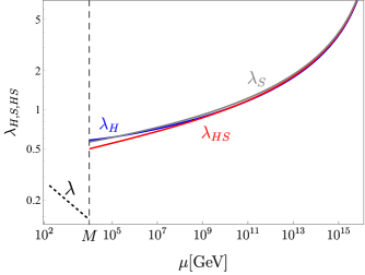
Figure 2: Evolution of the scalar quartic couplings, as explained in the text, for the same values as in Fig. 1. At the scale $M=10$ TeV the new particles decouple leaving a SM quartic coupling, given by Eq. (37), which runs up to the weak scale according to the SM RGE. For the chosen values this procedure gives finally $m_{h}=125\,$GeV.

We can repeat this procedure for different values of $p,\Lambda$ (and $\kappa$, $M$) and check if they are able to reproduce the measured values of $m_{t}\sim 173\,$GeV and $m_{h}\sim 125$ GeV.

In Fig. 3 we depict the region of $p,\Lambda$ that can reproduce values of $m_{t}$ in a region of $1$ GeV around $m_{t}=173$ GeV (band with green-pink colors) and $m_{h}$ in a region of 1 GeV around $m_{h}=125$ GeV (gray band). We do this for two values of $\kappa$ in each plot (for fixed $M=1\,$TeV on the right and $M=1000\,$TeV on the left). We see that, indeed, there is an overlapping region where one can reproduce both the Higgs boson and the top quark masses. For $M=1$ TeV this is found around $\Lambda\sim 10^{19}$ GeV, while for $M=1000\,$TeV the overlapping region occurs around $\Lambda\sim 10^{12}$ GeV. Larger values of $M$ lead to lower values of $\Lambda$ but for $M\gtrsim 10^{8}$ GeV there are no solutions. The effect of the exact scale at which we perform the matching between the complete model and the model with static scalars, which is parametrized by $\kappa=\Lambda/\Lambda_{\kappa}$, only changed the preferred value of $p$, which is always small, as required for consistency. We only represent values of $\Lambda$ a couple of orders of magnitude above $M$, since for $\Lambda$ close to $M$ the range of running is very small and the results are completely dominated by the matching, which cannot reliably be computed without knowing the details of the complete theory behind the four-fermion interactions.

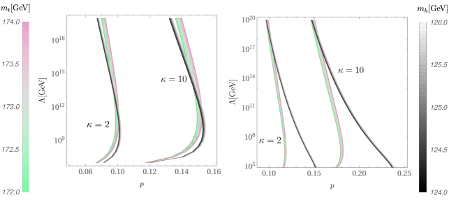
Figure 3: Region of $p,\Lambda$ that can reproduce values of $m_{t}$ in a region of $1$ GeV around $m_{t}=173$ GeV (band with green-pink colors) and $m_{h}$ in a region of 1 GeV around $m_{h}=125$ GeV (gray band). On the left for $M=1000\,$TeV and on the right for $M=1\,$TeV. In each plot we present results for two different values of $\kappa$.

Once $m_{t}$ and $m_{h}$ are obtained with the correct values, all the couplings and scales are quite constrained. However, the Majorana mass terms of the heavy fermions, $\mu_{\nu}$ and/or $\mu_{n}$, are completely free and can be adjusted to obtain neutrino masses below $1\,$eV using the inverse see-saw formula, Eq. (22). A complete analysis of neutrino masses, as for the rest of fermions, requires a three family analysis, but it is clear that given the freedom in $\mu_{\nu,n}$ there should be no problem for adjusting neutrino masses and mixings. Alternatively, one could also try to generate the Majorana mass terms by using composite scalars breaking lepton number as done in (Dib:2019iqo, ) with the interesting consequences discussed there.

IV Conclusions

Following previous work, Ref. (Krog:2015cna, ; Smetana:2013hm, ; Antusch:2002xh, ; Martin:1991xw, ), we have explored the possibility that the observed Higgs boson is mainly a bound state of neutrinos formed because a strong four-fermion interaction between neutrinos appears at high scales. The minimal version of this scenario has problems to reproduce the observed top quark mass and, especially, the Higgs boson mass. We have overcome these problems by introducing, in addition to right-handed neutrinos, $\nu_{R}$, a new singlet fermion, $n_{L}$, with four-fermion interactions $\left(\bar{\nu}_{R}n_{L}\right)\left(\bar{n}_{L}\nu_{R}\right)$, which gives rise to a new scalar bound state. This singlet scalar develops a VEV and, therefore, mixes with the Higgs doublet allowing us to obtain a small Higgs mass even if the couplings are large, as required in composite scalar models.

The compositeness condition basically fixes all Yukawa and quartic couplings at the compositeness scale, therefore, the parameters of the model are very constrained. In spite of that, this setup can accommodate the correct masses for the top quark and Higgs boson for compositeness scales below the Planck scale and masses of the new particles above the electroweak scale but below $\sim 10^{8}$ GeV.

If small Majorana masses are allowed for $\nu_{R}$ and/or $n_{L}$, we naturally obtain a low-scale see-saw scenario for neutrino masses with the presence of additional neutral scalars coupled to the neutral fermions. If the scale of the new particles is not much larger than $1$ TeV the model exhibits a very rich phenomenology that could be tested in present and near future experiments and will be studied in another publication. Further extensions in which the Majorana mass terms for $\nu_{R}$ and or $n_{L}$ are also generated by dynamical symmetry breaking might also be interesting.

Appendix A RGE of the model

Here we give the RGE beta functions of the model, which have been computed with the help of SARAH (Staub:2013tta, ) (we use the SU(5) convention $3g_{1}^{2}=5g^{\prime 2}$ for the U(1) factor)

Gauge couplings (same as in the SM):

$$\beta_{g_{1}}=\frac{41}{10}g_{1}^{3}\;,\qquad\beta_{g_{2}}=-\frac{19}{6}g_{2}^{3}\;,\qquad\beta_{g_{3}}=-7g_{3}^{3}$$ (40)

Yukawas:

$$\beta_{y_{t}} =y_{t}\left(\frac{9}{2}y_{t}^{2}-8g_{3}^{2}-\frac{9}{4}g_{2}^{2}-\frac{17}{20}g_{1}^{2}+y_{\nu}^{2}\right)$$

$$\beta_{y_{\nu}} =y_{\nu}\left(\frac{5}{2}y_{\nu}^{2}+\frac{1}{2}y_{s}^{2}+3y_{t}^{2}-\frac{9}{20}\left(5g_{2}^{2}+g_{1}^{2}\right)\right)$$ (41)

$$\beta_{y_{s}} =y_{s}\left(2y_{s}^{2}+y_{\nu}^{2}\right)$$

Quartic couplings:

$$\beta_{\lambda_{H}} =12\lambda_{H}^{2}+\frac{27}{100}g_{1}^{4}+\frac{9}{10}g_{1}^{2}g_{2}^{2}+\frac{9}{4}g_{2}^{4}+\lambda_{H}\left(12y_{t}^{2}-\frac{9}{5}g_{1}^{2}-9g_{2}^{2}+4y_{\nu}^{2}\right)+2\lambda_{HS}^{2}-4y_{\nu}^{4}-12y_{t}^{4}$$

$$\beta_{\lambda_{S}} =10\lambda_{S}^{2}+4\lambda_{S}y_{s}^{2}+4\lambda_{HS}^{2}-4y_{s}^{4}$$ (42)

$$\beta_{\lambda_{HS}} =\lambda_{HS}\left(4\lambda_{HS}+6\lambda_{H}+4\lambda_{S}+2y_{\nu}^{2}+2y_{s}^{2}+6y_{t}^{2}-\frac{9}{10}g_{1}^{2}-\frac{9}{2}g_{2}^{2}\right)-4y_{s}^{2}y_{\nu}^{2}$$

References

- (1) W. A. Bardeen, C. T. Hill and M. Lindner, Minimal Dynamical Symmetry Breaking of the Standard Model, Phys. Rev. D41 (1990) 1647.
- (2) Y. Nambu and G. Jona-Lasinio, DYNAMICAL MODEL OF ELEMENTARY PARTICLES BASED ON AN ANALOGY WITH SUPERCONDUCTIVITY. II, Phys. Rev. 124 (1961) 246.
- (3) Y. Nambu and G. Jona-Lasinio, Dynamical Model of Elementary Particles Based on an Analogy with Superconductivity. 1., Phys. Rev. 122 (1961) 345.
- (4) V. A. Miransky, M. Tanabashi and K. Yamawaki, Dynamical Electroweak Symmetry Breaking with Large Anomalous Dimension and t Quark Condensate, Phys. Lett. B221 (1989) 177.
- (5) V. A. Miransky, M. Tanabashi and K. Yamawaki, Is the t Quark Responsible for the Mass of W and Z Bosons?, Mod. Phys. Lett. A4 (1989) 1043.
- (6) M. Suzuki, Composite Higgs Bosons in the Nambu-Jona-Lasinio Model, Phys. Rev. D41 (1990) 3457.
- (7) M. Suzuki, Formation of Composite Higgs Bosons From Quark - Anti-quarks at Lower Energy Scales, Mod. Phys. Lett. A5 (1990) 1205.
- (8) W. J. Marciano, Dynamical Symmetry Breaking and the Top Quark Mass, Phys. Rev. D41 (1990) 219.
- (9) W. J. Marciano, HEAVY TOP QUARK MASS PREDICTIONS, Phys. Rev. Lett. 62 (1989) 2793.
- (10) C. T. Hill, Quark and Lepton Masses from Renormalization Group Fixe d Points, Phys. Rev. D24 (1981) 691.
- (11) C. T. Hill, C. N. Leung and S. Rao, Renormalization Group Fixed Points and the Higgs Boson Spectrum, Nucl. Phys. B262 (1985) 517.
- (12) G. Cvetic, Top quark condensation, Rev. Mod. Phys. 71 (1999) 513 [hep-ph/9702381].
- (13) C. T. Hill and E. H. Simmons, Strong dynamics and electroweak symmetry breaking, Phys. Rept. 381 (2003) 235 [hep-ph/0203079].
- (14) J. Krog and C. T. Hill, Is the Higgs Boson Composed of Neutrinos?, Phys. Rev. D92 (2015) 093005 [1506.02843].
- (15) A. Smetana, Top-quark and neutrino composite Higgs bosons, Eur. Phys. J. C73 (2013) 2513 [1301.1554].
- (16) S. Antusch, J. Kersten, M. Lindner and M. Ratz, Dynamical electroweak symmetry breaking by a neutrino condensate, Nucl. Phys. B658 (2003) 203 [hep-ph/0211385].
- (17) S. P. Martin, Dynamical electroweak symmetry breaking with top quark and neutrino condensates, Phys. Rev. D44 (1991) 2892.
- (18) C. Dib, S. Kovalenko, I. Schmidt and A. Smetana, Low-scale seesaw from neutrino condensation, 1904.06280.
- (19) G. Barenboim and C. Bosch, Composite states of two right-handed neutrinos, Phys. Rev. D94 (2016) 116019 [1610.06588].
- (20) G. Barenboim and J. Rasero, Baryogenesis from a right-handed neutrino condensate, JHEP 03 (2011) 097 [1009.3024].
- (21) G. Barenboim, Inflation might be caused by the right: Handed neutrino, JHEP 03 (2009) 102 [0811.2998].
- (22) R. N. Mohapatra, Mechanism for Understanding Small Neutrino Mass in Superstring Theories, Phys. Rev. Lett. 56 (1986) 561.
- (23) R. N. Mohapatra and J. W. F. Valle, Neutrino Mass and Baryon Number Nonconservation in Superstring Models, Phys. Rev. D34 (1986) 1642.
- (24) D. Wyler and L. Wolfenstein, Massless Neutrinos in Left-Right Symmetric Models, Nucl. Phys. B218 (1983) 205.
- (25) J. Bernabeu, A. Santamaria, J. Vidal, A. Mendez and J. W. F. Valle, Lepton Flavor Nonconservation at High-Energies in a Superstring Inspired Standard Model, Phys. Lett. B187 (1987) 303.
- (26) B. A. Kniehl and O. L. Veretin, Two-loop electroweak threshold corrections to the botto m and top Yukawa couplings, Nucl. Phys. B885 (2014) 459 [1401.1844].
- (27) R. Hempfling and B. A. Kniehl, On the relation between the fermion pole mass and MS Yukawa coupling in the standard model, Phys. Rev. D51 (1995) 1386 [hep-ph/9408313].
- (28) B. Patt and F. Wilczek, Higgs-field portal into hidden sectors, hep-ph/0605188.
- (29) J. McDonald, Gauge singlet scalars as cold dark matter, Phys. Rev. D50 (1994) 3637 [hep-ph/0702143].
- (30) V. Silveira and A. Zee, SCALAR PHANTOMS, Phys. Lett. 161B (1985) 136.
- (31) P. S. B. Dev and A. Pilaftsis, Minimal Radiative Neutrino Mass Mechanism for Inverse Seesaw Models, Phys. Rev. D86 (2012) 113001 [1209.4051].
- (32) Y. Chikashige, R. N. Mohapatra and R. D. Peccei, Are There Real Goldstone Bosons Associated with Broken Lepton Number?, Phys. Lett. 98B (1981) 265.
- (33) G. B. Gelmini and M. Roncadelli, Left-Handed Neutrino Mass Scale and Spontaneously Broke n Lepton Number, Phys. Lett. 99B (1981) 411.
- (34) S. Bertolini and A. Santamaria, The Doublet Majoron Model and Solar Neutrino Oscillations, Nucl. Phys. B310 (1988) 714.
- (35) A. Sirlin and R. Zucchini, Dependence of the Quartic Coupling H(m) on M() and the Possible Onset of New Physics in the Higgs Sector of the Standard Model, Nucl. Phys. B266 (1986) 389.
- (36) C. Dib, S. Kovalenko, I. Schmidt and A. Smetana, Low-scale seesaw from neutrino condensation, AIP Conf. Proc. 2165 (2019) 020023.
- (37) F. Staub, SARAH 4 : A tool for (not only SUSY) model builders, Comput. Phys. Commun. 185 (2014) 1773 [1309.7223].