Helical massive fermions under rotation

Abstract

The properties of a massive fermion field undergoing rigid rotation at finite temperature and chemical potential are discussed. The polarisation imbalance is taken into account by considering a helicity chemical potential, which is dual to the helicity charge operator. The advantage of the proposed approach is that, as opposed to the axial current, the helicity charge current remains conserved at finite mass. A computation of thermal expectation values of the vector, helicity and axial charge currents, as well as of the fermion condensate and stress-energy tensor is provided. In all cases, analytic constitutive equations are derived for the non-equilibrium transport terms, as well as for the quantum corrections to the equilibrium terms (which are derived using an effective relativistic kinetic theory model for fermions with helicity imbalance) in the limit of small masses. In the context of the parameters which are relevant to relativistic heavy ion collisions, the expressions derived in the massless limit are shown to remain valid for masses up to the thermal energy, except for the axial charge conductivity in the azimuthal direction, which presents strong variations with the particle mass.

1 Introduction

Quantum systems undergoing rigid rotation have been the object of academic study since the late ’70s, when Vilenkin showed that, due to the spin-orbit coupling, more anti-neutrinos would be emitted on the direction which is parallel to the angular momentum vector of a rotating black hole. Conversely, an excess of neutrinos would be emitted on the anti-parallel direction vilenkin78 . Recently, evidence from relativistic heavy–ion collisions experiments suggests that a global polarisation of the medium formed following the collision can be highlighted by looking at the decay products of the $\Lambda$ hyperons star17nat ; star18prc . Such measurements can provide quantitative validation of models describing polarization of strongly interacting matter induced through various mechanisms kharzeev16 , such as the chiral vortical effect rogachevsky10 ; baznat13 ; baznat18 and the chiral magnetic effect fukushima08 ; braguta14 .

The past decade has seen many attempts to extend the standard thermal field theory, in which the canonical thermodynamic variables are the temperature four-vector $\beta^{\mu}=u^{\mu}/T$ (given as the ratio between the local four-velocity of the fluid, $u^{\mu}$, and its temperature, $T$) and chemical potentials related to the electric or baryon charges, to also incorporate polarisation-related charges. Some recent examples include the recent results in Ref. buzzegoli18 , where the excess is taken into account by means of an axial chemical potential, $\mu_{A}$, coupled with the axial charge current; and Ref. becattini19 , where it is suggested that an extra chemical potential, called the spin potential, could explain a polarisation excess through a coupling with the spin tensor.

There are two major drawbacks of the aforementioned approaches. First, the axial current $J^{\mu}_{A}=\overline{\psi}\gamma^{\mu}\gamma^{5}\psi$ can be used to define a classically conserved axial charge, $Q_{A}$, only for massless fermions. In the case of massive particles, $J^{\mu}_{A}$ is no longer conserved. Second, the spin tensor (or its contraction with a constant spin potential) does not commute with the Dirac equation, which implies that its eigenfunctions are not solutions of the Dirac equation.

In this paper, an alternative to the axial charge current and spin tensor extensions of canonical thermal field theory is employed, which is based on the helicity charge current, introduced in Ref. helican . The advantage of the present approach is that the helicity charge current remains conserved for massive fermions and thus, one can consider the helicity operator $h$ (related to the temporal component of the Pauli-Lubanski vector operator) as a natural alternative to the chirality operator for the regime of non-vanishing mass. It is defined through:

$$h=\frac{\bm{S}\cdot\bm{P}}{p},$$ (1)

where $\bm{S}$ and $\bm{P}=-i\nabla$ are the spin and momentum operators, while $p=|\bm{P}|=\sqrt{-\Delta}$ is the momentum magnitude (for a discussion on the properties of the fractional Laplacian, see Ref. pozrikidis16 ). The eigenvalues of $h$ are $1/2$ and $-1/2$, distinguishing between right-handed and left-handed helicity particles, respectively. At the relativistic quantum mechanics level, $h$ commutes with the Hamiltonian $H$ of the free Dirac field. With the help of $h$, it is possible to introduce the helicity charge current (HCC),

$$J^{\mu}_{H}=\overline{\psi}\gamma^{\mu}h\psi+\overline{h\psi}\gamma^{\mu}\psi,$$ (2)

which is classically conserved when $\psi$ is a solution of the free Dirac equation. The associated time-independent charge, $Q_{H}$, can be associated to a helicity chemical potential $\mu_{H}$, which accounts for an overall helicity bias.

Despite the apparent non-locality of $h$ due to the factor $p^{-1}$ in its definition, the helicity can be regarded as a “good” quantum number in quantum field theory. It has been routinely employed in canonical second quantisation to characterise particle states and for scattering processes in quantum electrodynamics (QED) itzykson80 ; weinberg95 ; peskin95 . In quantum chromodynamics (QCD), the total quark helicity is conserved under the interactions due to the vector couplings with the gluon fields when the quarks are massless brodsky89 ; kapusta20arxiv , which is a good approximation in the high-temperature quark-gluon plasma (QGP) formed in heavy-ion collisions (HIC). Furthermore, the effects due to the helicity and spin imbalance in the QGP can be expected to be of similar importance, since their equilibration times are of a similar order of magnitude ruggieri16prd ; kapusta20prc .

This paper presents an analysis of the quantum thermal expectation values (t.e.v.s) of the vector and helicity charge currents (VCC and HCC), axial charge current (ACC), fermion condensate (FC) and stress-energy tensor (SET) corresponding to the free massive Dirac field in rigid rotation with angular velocity $\bm{\Omega}$, at finite vector ($\mu_{V}$) and helicity ($\mu_{H}$) chemical pontentials. It comes as an extension to the finite mass regime of Ref. helican , where the same quantities were investigated for massless fermions, in the presence of the vector ($\mu_{V}$), axial ($\mu_{A}$) and helical ($\mu_{H}$) chemical potentials. However, since the axial current $J^{\mu}_{A}=\overline{\psi}\gamma^{\mu}\gamma^{5}\psi$ is not conserved for fermions of nonvanishing mass $M$ ($\partial_{\mu}J^{\mu}_{A}=2iM\overline{\psi}\gamma^{5}\psi$), the axial chemical potential cannot be consistently introduced as a thermodynamic variable ruggieri20 and is thus assumed to vanish in this paper.

The t.e.v.s mentioned in the previous paragraph are computed as traces over Fock space, weighted by the density operator ${\hat{\varrho}}$ defining the thermal state. For global equilibrium states, such as the rigid rotation, ${\hat{\varrho}}$ can be written down in a straightforward manner with respect to conserved operators vilenkin80 ; itzykson80 ; kapusta89 ; laine16 ; mallik16 . Specifically, when $\bm{\Omega}$ is parallel to the $z$ axis, ${\hat{\varrho}}$ is given by vilenkin80

$${\hat{\varrho}}=\exp\left[-\beta_{0}(\widehat{H}-\Omega\widehat{M}^{z}-\mu_{V;0}\widehat{Q}_{V}-\mu_{H;0}\widehat{Q}_{H})\right],$$ (3)

where $\widehat{H}$, $\widehat{\bm{M}}$, $\widehat{Q}_{V}$ and $\widehat{Q}_{H}$ are the Hamiltonian, total angular momentum, vector charge and helicity charge operators, respectively. In non-equilibrium situations, the Zubarev formalism can be employed to consistently define the density operator zubarev79 ; becattini15 ; mallik16 ; buzzegoli18 ; buzzegoli20phd . Several by-now traditional approaches can be employed for the analysis of rotating systems at finite temperature, including direct mode sums vilenkin80 ; casals12 ; ambrus14plb , point splitting birrell82 ; duffy03 ; panerai16 ; ambrus16prd and the perturbative approach based on Kubo formulae in the imaginary jeon95 ; kharzeev09prd ; landsteiner11prl ; laine16 or real schwinger61 ; keldysh65 ; danielewicz84 ; mallik16 time formalism. Full advantage may be taken of the standard diagramatics techniques in the perturbative approach by employing the Fourier transform to the momentum space. However, this comes at the cost that the rotation part of ${\hat{\varrho}}$, $-\beta_{0}\Omega\widehat{M}^{z}$, must be treated perturbatively, since $\widehat{M}^{z}$ does not commute with $\widehat{\bm{P}}$ and is therefore not diagonal with respect to the momentum eigenmodes landsteiner13lnp ; becattini15 ; buzzegoli18 .

In this paper, the mode sum approach is employed to exactly compute the Fock space trace weighted by ${\hat{\varrho}}$ introduced in Eq. (3). The key ingredient is the expansion of the field operator $\widehat{\Psi}$ with respect to the set of modes which are simultaneous eigenfunctions of the Hamiltonian $H$, linear ($P^{z}$) and angular momentum ($M^{z}$) operators along $\bm{\Omega}$ and helicity operator $h$ ambrus14plb ; jiang16 ; ambrus16prd ; ebihara17plb ; chernodub17njl ; chernodub17edge ; ambrus19lnp . With respect to this basis, ${\hat{\varrho}}$ is diagonal and the thermal average is straightforward to compute. Without resorting to perturbative expansions, the present approach yields exact integral expressions which are amenable to numerical integration for general values of the fermion mass $M$. In addition, analytic results are derived for all quantities, which are either exact at small mass at any distance from the rotation axis, or they are exact for any mass on the rotation axis. A similar method was used in Ref. helican for massless fermions.

A consequence of taking the non-perturbative approach is that the vacuum state must be carefully defined. As pointed out in the early ’80s by Iyer iyer82 , the vacuum state of a fermion field corresponding to an observer undergoing rigid rotation differs in general from the stationary, Minkowski vacuum. The rotating vacuum proposed by Iyer treats as particle modes those modes for which the co-rotating energy $\widetilde{E}=E-\Omega m$ (where $E$ is the Minkowksi energy and $m$ is the eigenvalue of $M^{z}$) is positive. In general, this choice includes modes with negative Minkowksi energy, $E<0$. This is contrary to the case of the Klein-Gordon field, where the stationary vacuum is the only possible choice for observers undergoing rigid rotation letaw80 ; letaw81 ; duffy03 ; ambrus14plb . Moreover, the non-perturbative analysis of rigidly-rotating thermal states at finite temperature of the scalar field is not possible, since the t.e.v.s diverge due to the behaviour of the Bose-Einstein distribution $(e^{\widetilde{E}/T}-1)^{-1}$ when $\widetilde{E}\rightarrow 0$ kay91 ; ottewill00prd ; ottewill00pla ; ambrus14plb . When the rotating and Minkowski vacua do not coincide, the t.e.v.s computed with respect to the former exhibit temperature-independent contributions vilenkin79 ; vilenkin80 ; ambrus14plb ; ambrus19lnp . It is worth mentioning that the modes with $E\widetilde{E}<0$ (giving rise to the difference between the stationary and rotating vacua) can be eliminated with appropriate boundary conditions, e.g. by enclosing the system inside a boundary duffy03 ; ambrus16prd or when the space-time itself is bounded and the rotation parameter is sufficiently small nicolaevici01 ; ambrus16prd ; ambrus16prd2 ; ambrus19apa .

As a classical (i.e., non-quantum) reference theory, a simple kinetic model based on the Fermi-Dirac distribution is proposed, which takes into account the helicity bias by means of $\mu_{H}$. Unsurprisingly, the classical analysis predicts a perfect fluid behaviour, as expected since rigid-rotation is a global thermodynamic equilibrium solution in relativistic kinetic theory. This thermal equilibrium state is fully characterised by means of the vector $Q_{V}^{\rm RKT}$ and helicity $Q_{H}^{\rm RKT}$ charge densities, the energy density $E_{\rm RKT}$ and the pressure $P_{\rm RKT}$.

At the quantum level, the hydrodynamic content of the charge currents and the SET is extracted with the aid of the $\beta$ (thermometer) frame van12 ; van13 ; landsteiner13lnp ; becattini15epjc , in which the four velocity is that corresponding to rigid rotation. The Landau frame can also be defined landsteiner11jhep ; ambrus17plb ; buzzegoli18 , but it is more cumbersome to use in the present context. In the $\beta$ frame, the quantum corrections $\Delta Q_{V/H}(M)$, $\Delta E(M)$ and $\Delta P(M)$, taken with respect to the classical equilibrium quantities $Q^{\rm RKT}_{V/H}(M)$, $E_{\rm RKT}(M)$ and $P_{\rm RKT}(M)$, are investigated as functions of $M$. These quantum corrections are quadratic with respect to the vorticity parameter $\Omega$. The terms that deviate from the perfect fluid form describe anomalous transport phenomena in the form of rest frame charge and heat fluxes. These fluxes are characterised using the vortical charge and heat conductivities, $\sigma^{\omega}_{\ell}$ ($\ell\in\{V,A,H\}$) and $\sigma^{\omega}_{\varepsilon}$, as well as the circular charge and heat conductivities, $\sigma^{\tau}_{\ell}$ and $\sigma^{\tau}_{\varepsilon}$. These conductivities are computed analytically and numerically, reducing for $M=0$ to the $\mu_{A}=0$ limit of the results derived in Ref. helican . The robustness of the analytic expressions for the quantum corrections and conductivities is probed in the case of non-vanishing mass in the parameter regime which is prevalent in ultrarelativistic heavy ion collisions (labelled “HIC” throughout this paper), namely temperature $T=150\ {\rm MeV}$ jacak12 , vector chemical potential $\mu_{V}=30\ {\rm MeV}$ huang12 (considering that $\mu_{V}=\mu_{B}/3$, where $\mu_{B}$ is the baryonic chemical potential) and $\Omega=6.6\ {\rm MeV}$ (corresponding to $10^{22}\,{\rm s}^{-1}$ star17nat ; wang17 ).

Before ending the introduction, it is worth pointing out that, since the helicity for a massive particle is not a Lorentz invariant property, the theory involving the helicity chemical potential becomes frame-dependent. The relevance of such a formulation can be seen in the case of systems that explicitly break Lorentz invariance, such as the confined state encountered in a single nucleus or the quark-gluon plasma (QGP) undergoing rigid rotation.

The outline of the paper is as follows. Preliminaries regarding the kinematics of rigidly-rotating states are introduced in Sec. 2, where the kinematic tetrad consisting of the local velocity $u^{\mu}$, acceleration $a^{\mu}$, vorticity $\omega^{\mu}$ and a fourth vector $\tau^{\mu}$ is introduced. The helicity current is introduced in Sec. 3. The kinetic theory model taking into account the helicity bias is formulated in Sec. 4. The finite temperature field theory formalism employed in this paper is summarised in Sec. 5 and the t.e.v.s of the vector and helicity charge currents (VCC and HCC), axial charge current (ACC), fermion condensate (FC) and stress-energy tensor (SET) are discussed in Sections 6, 7, 8 and 9, respectively. Section 10 concludes this paper. Planck units are employed throughout this paper, such that $\hbar=k_{B}=c=1$, while the Minkowski metric signature is taken as $(+,-,-,-)$. The Levi-Civita symbol is defined such that $\varepsilon^{0123}=(-g)^{-1/2}$.

2 Kinematics of rigid rotation

Figure 1: Schematic representation of the kinematic tetrad corresponding to a fluid undergoing rigid rotation with respect to the vertical axis, with angular velocity $\bm{\Omega}=\Omega\bm{e}_{z}$. The drawing on the left shows the spatial components of the vectors $\bm{u}$, $\bm{a}$, $\bm{\omega}$ and $\bm{\tau}$ forming the orthogonal tetrad, pointing along the azimuthal, radial, vertical and again azimuthal directions, respectively. The drawing on the right depicts the spacetime representation of the four-velocity ($u$) and the vector $\tau$.

The analysis in this paper is focussed on states undergoing rigid rotation about the $z$ axis. The properties of such states are most conveniently expressed with respect to cylindrical coordinates. For future convenience, the following tetrad is introduced:

$$e_{\hat{t}}= \partial_{t}, e_{\hat{\rho}}= \partial_{\rho}, e_{\hat{\varphi}}= \rho^{-1}\partial_{\varphi}, e_{\hat{z}}=\partial_{z},$$

$$\omega^{\hat{t}}= dt, \omega^{\hat{\rho}}= d\rho, \omega^{\hat{\varphi}}= \rho\,d\varphi, \omega^{\hat{z}}=dz.$$ (4)

In what follows, hatted indices are employed to refer to vector (or tensor) components expressed with respect to the above tetrad.

The four-velocity of a fluid undergoing rigid rotation can be written as:

$$u=\Gamma(\partial_{t}+\Omega\partial_{\varphi})=\Gamma(e_{\hat{t}}+\rho\Omega e_{\hat{\varphi}}),$$ (5)

such that its components with respect to the coordinate indices and with respect to the tetrad satisfy

$$u^{\hat{t}}=u^{t}=\Gamma,\qquad u^{\hat{\varphi}}=\rho u^{\varphi}=\rho\Omega\Gamma.$$ (6)

The Lorentz factor $\Gamma$,

$$\Gamma=(1-\rho^{2}\Omega^{2})^{-1/2},$$ (7)

diverges as $\rho\rightarrow\rho_{\rm SLS}$, where $\rho_{\rm SLS}$ is the distance from the rotation axis to the speed of light surface (SLS), on which the rigidly-rotating fluid rotates at the speed of light. It is given by:

$$\rho_{\rm SLS}=\Omega^{-1}.$$ (8)

Aside from the tetrad introduced in Eq. (4), it is convenient to define another tetrad, comprised of kinematic quantities derived from the four-velocity becattini15 ; becattini15epjc . Starting from the expression (5) for $u=u^{\hat{\alpha}}e_{\hat{\alpha}}$, the four-acceleration can be defined via:

$$a=\nabla_{u}u=a^{\hat{\rho}}e_{\hat{\rho}},\qquad a^{\hat{\rho}}=-\rho\Omega^{2}\Gamma^{2}.$$ (9)

It can be seen that $a\cdot u=0$ by construction. Taking into account the following expression for the gradient of the velocity vector,

$$\nabla_{\hat{\alpha}}u_{\hat{\beta}}=\Omega\Gamma\begin{pmatrix}0&0&0&0\\ \rho\Omega\Gamma^{2}&0&-\Gamma^{2}&0\\ 0&1&0&0\\ 0&0&0&0\end{pmatrix},$$ (10)

the kinematic vorticity vector, $\omega=\omega^{\hat{\alpha}}e_{\hat{\alpha}}$, can be defined through:

$$\omega=\frac{1}{2}\varepsilon^{{\hat{\alpha}}{\hat{\beta}}{\hat{\gamma}}{\hat{\sigma}}}e_{{\hat{\alpha}}}u_{\hat{\beta}}\nabla_{\hat{\gamma}}u_{\hat{\sigma}}=\omega^{\hat{z}}e_{\hat{z}},\qquad\omega^{\hat{z}}=\Gamma^{2}\Omega,$$ (11)

where the Levi-Civita tensor satisfies $\varepsilon^{\hat{0}\hat{1}\hat{2}\hat{3}}=+1$. It can be seen that $\omega\cdot u=0$ by construction. Moreover, in the case of rigid rotation, when the acceleration is given by Eq. (9), $\omega$ is orthogonal to both $u$ and $a$. A fourth vector which is orthogonal to $u$, $a$ and $\omega$ is (our definition differs from the one in Refs. becattini15 ; becattini15epjc by a minus sign)

$$\tau^{\hat{\alpha}}=-\varepsilon^{{\hat{\alpha}}{\hat{\beta}}{\hat{\gamma}}{\hat{\sigma}}}\omega_{\hat{\beta}}a_{\hat{\gamma}}u_{\hat{\sigma}},\qquad\tau=-\rho\Omega^{3}\Gamma^{5}(\rho\Omega e_{\hat{t}}+e_{\hat{\varphi}}).$$ (12)

It can be seen that the vectors $u$, $a$, $\omega$ and $\tau$ comprise an orthogonal tetrad. The squared norms of these vectors are given below:

$$u^{2}= 1, \tau^{2}= -\Omega^{4}\Gamma^{6}(\Gamma^{2}-1),$$

$$\omega^{2}= -\bm{\omega}^{2}=-\Omega^{2}\Gamma^{4}, a^{2}= -\bm{a}^{2}=-\Omega^{2}\Gamma^{2}(\Gamma^{2}-1).$$ (13)

Figure 1 shows a schematic representation of these four vectors.

3 Charge currents and conserved charges

3.1 Classical theory

The free Dirac field is described by the following Lagrangian:

$$L_{\rm free}=\frac{i}{2}(\overline{\psi}\gamma^{\mu}\partial_{\mu}\psi-\overline{\partial_{\mu}\psi}\gamma^{\mu}\psi)-M\overline{\psi}\psi,$$ (14)

where $M$ is the mass of the field quanta, $\psi$ is the Dirac 4-component spinor, $\overline{\psi}=\psi^{\dagger}\gamma^{0}$ is its Dirac adjoint and $\gamma^{\mu}$ are the $4\times 4$ gamma matrices. For definiteness, these matrices together with the fifth gamma matrix, $\gamma^{5}=i\gamma^{0}\gamma^{1}\gamma^{2}\gamma^{3}$, are taken in the Dirac representation:

$$\gamma^{0}=\begin{pmatrix}1&0\\ 0&-1\end{pmatrix},\qquad\gamma^{i}=\begin{pmatrix}0&\sigma^{i}\\ -\sigma^{i}&0,\end{pmatrix},\qquad\gamma^{5}=\begin{pmatrix}0&1\\ 1&0\end{pmatrix},$$ (15)

where $\sigma^{i}$ are the Pauli matrices, given by:

$$\sigma^{1}=\begin{pmatrix}0&1\\ 1&0\end{pmatrix},\qquad\sigma^{2}=\begin{pmatrix}0&-i\\ i&0\end{pmatrix},\qquad\sigma^{3}=\begin{pmatrix}1&0\\ 0&-1\end{pmatrix}.$$ (16)

Noting that the spin matrix satsfies

$$S^{k}=\frac{i}{8}\varepsilon^{0ijk}[\gamma_{i},\gamma_{j}]=\frac{1}{2}\begin{pmatrix}\sigma^{k}&0\\ 0&\sigma^{k}\end{pmatrix},$$ (17)

the helicity $h$, introduced in Eq. (1) can be shown to satisfy helican

$$h=\frac{1}{p}W^{0}=\frac{\bm{S}\cdot\bm{P}}{p}=\gamma^{5}\gamma^{0}\frac{\bm{\gamma}\cdot\bm{P}}{2p},$$ (18)

where $p=|\bm{p}|$ represents the momentum magnitude. In Eq. (18), $W^{0}$ is the zeroth component of the Pauli-Lubanski vector, defined as itzykson80

$$W^{\mu}=-\frac{1}{2}\varepsilon^{\mu\alpha\beta\lambda}M_{\alpha\beta}P_{\lambda},$$ (19)

which is expressed in terms of the total angular momentum operator $M_{\alpha\beta}=x_{\alpha}P_{\beta}-x_{\beta}P_{\alpha}+S_{\alpha\beta}$ and the momentum operator $P_{\lambda}=i\partial_{\lambda}$, where $S_{\alpha\beta}=\frac{i}{4}[\gamma_{\alpha},\gamma_{\beta}]$. It can be shown that the eigenvalues of $h$ are $\lambda=\pm 1/2$ itzykson80 .

The Dirac equation for the spinor $\psi$ and its adjoint $\overline{\psi}$ can be obtained using the Euler-Lagrange formalism, starting from the Lagrangian in Eq. (14):

$$i\not{\partial}\psi=M\psi,\qquad i\overline{\not{\partial}\psi}=-M\overline{\psi},$$ (20)

where $\not{a}\equiv\gamma^{\mu}a_{\mu}$ is the Feynman slash notation. The Dirac inner product of two 4-spinors $\psi$ and $\chi$ can be introduced as:

$$\braket{\psi,\chi}=\int d^{3}x\,\overline{\psi}\gamma^{0}\chi,$$ (21)

being time independent when $\psi$ and $\chi$ satisfy the Dirac equation (20).

The vector (VCC), axial (ACC) and helical (HCC) charge currents, denoted $J^{\mu}_{V}$, $J^{\mu}_{A}$ and $J^{\mu}_{H}$, respectively, can be introduced as follows helican :

$$J^{\mu}_{V}=\overline{\psi}\gamma^{\mu}\psi,\qquad J^{\mu}_{A}=\overline{\psi}\gamma^{\mu}\gamma^{5}\psi,\qquad J^{\mu}_{H}=\overline{\psi}\gamma^{\mu}h\psi+\overline{h\psi}\gamma^{\mu}\psi.$$ (22)

To see the connection between the axial and helical charge currents, let $\psi=\psi_{R}+\psi_{L}=\psi_{\uparrow}+\psi_{\downarrow}$, where $\psi_{R/L}=\frac{1}{2}(1\pm\gamma^{5})\psi$ and $\psi_{\uparrow/\downarrow}=(\frac{1}{2}\pm h)\psi$. With this split, it can be seen that the axial and helical currents receive positive contributions from the right-chiral and right-helicity states, and negative contributions from the left-chiral and left-helicity states, respectively, as follows:

$$J^{\mu}_{A}=\overline{\psi}_{R}\gamma^{\mu}\psi_{R}-\overline{\psi}_{L}\gamma^{\mu}\psi_{L},\qquad J^{\mu}_{H}=\overline{\psi}_{\uparrow}\gamma^{\mu}\psi_{\uparrow}-\overline{\psi}_{\downarrow}\gamma^{\mu}\psi_{\downarrow}.$$ (23)

Assuming that $\psi$ satisfies Eq. (20), it is straightforward to see that $\partial_{\mu}J^{\mu}_{V}=0$ and thus, the vector current is classically conserved. For $J^{\mu}_{A}$, the mass term in Eq. (20) breaks the conservation:

$$\partial_{\mu}J^{\mu}_{A}=(iM\overline{\psi})\gamma^{5}\psi+\overline{\psi}\gamma^{5}(iM\psi)=2iM\overline{\psi}\gamma^{5}\psi.$$ (24)

Since $[P^{\mu},W^{\nu}]=0$, it can be seen that the divergence of $J^{\mu}_{H}$ is given by:

$$\partial_{\mu}J^{\mu}_{H}=\overline{\psi}[\gamma^{\mu},h]\partial_{\mu}\psi+\overline{[\gamma^{\mu},h]\partial_{\mu}\psi}\psi=0,$$ (25)

where the last equation follows after noting that $[\gamma^{0},h]=0$, while

$$[\gamma^{i},h]=-\frac{2i}{p}\gamma^{5}\gamma^{0}\varepsilon^{0ijk}P_{j}S_{k}=\frac{i}{p}\varepsilon^{0ijk}P_{j}\gamma_{k}.$$ (26)

Thus, it can be seen that

$$[\gamma^{\mu},h]\partial_{\mu}\psi=-i[\gamma^{\mu},h]P_{\mu}\psi=\frac{1}{p}\varepsilon^{0ijk}P_{j}\gamma_{k}P_{i}\psi=0.$$ (27)

The associated charges can be computed by integrating the zeroth components of the currents with respect to $d^{3}x$. The following expressions are obtained:

$$Q_{V}=\int d^{3}x\,\psi^{\dagger}\psi,\qquad Q_{A}=\int d^{3}x\,\psi^{\dagger}\gamma^{5}\psi,\qquad Q_{H}=2\int d^{3}x\,\psi^{\dagger}h\psi.$$ (28)

To prove the last equality, it is convenient to consider the spatial Fourier decomposition of $\psi(t,\bm{x})$,

$$\psi(t,\bm{x})=\int\frac{d^{3}p}{(2\pi)^{3}}e^{i\bm{p}\cdot\bm{x}}\psi_{\bm{p}}(t),\qquad h\psi(t,\bm{x})=\int\frac{d^{3}p}{(2\pi)^{3}}e^{i\bm{p}\cdot\bm{x}}\frac{\bm{S}\cdot\bm{p}}{p}\psi_{\bm{p}}(t).$$ (29)

This allows $Q_{H}$ to be written as

$$Q_{H}=\int\frac{d^{3}p}{(2\pi)^{3}}\left(\overline{\psi}_{\bm{p}}\gamma^{0}\frac{\bm{S}\cdot\bm{p}}{p}\psi_{\bm{p}}+\overline{\frac{\bm{S}\cdot\bm{p}}{p}\psi_{\bm{p}}}\gamma^{0}\psi_{\bm{p}}\right).$$ (30)

Noting that $\overline{\bm{S}}=\bm{S}$ and $[\bm{S},\gamma^{0}]=0$, the second term in the above integrand can be seen to be equal to the first. Applying the inverse Fourier transform recovers Eq. (28).

The charges $Q_{\ell}$ ($\ell\in\{V,A,H\}$) can be shown to satisfy:

$$\partial_{t}Q_{V}=0,\qquad\partial_{t}Q_{A}=2iM\int d^{3}x\,\overline{\psi}\gamma^{5}\psi,\qquad\partial_{t}Q_{H}=0.$$ (31)

Thus, at the classical level and at arbitrary mass $M$, only the vector and helical charges, $Q_{V}$ and $Q_{H}$, are conserved.

3.2 Charge operators

After second quantization, $\psi$ is promoted to a quantum operator $\widehat{\Psi}$. The operator versions of the vector (VCC), axial (ACC) and helical (HCC) charge currents introduced in Eq. (22) reads

$$\widehat{J}^{\mu}_{V}=\frac{1}{2}[\widehat{\overline{\Psi}},\gamma^{\mu}\widehat{\Psi}],\qquad\widehat{J}^{\mu}_{A}=\frac{1}{2}[\widehat{\overline{\Psi}},\gamma^{\mu}\gamma^{5}\widehat{\Psi}],\qquad\widehat{J}^{\mu}_{H}=\frac{1}{2}[\widehat{\overline{\Psi}},\gamma^{\mu}h\widehat{\Psi}]+\frac{1}{2}[\widehat{\overline{h\Psi}},\gamma^{\mu}\widehat{\Psi}],$$ (32)

where the commutators were introduced to avoid operator ordering ambiguities. In order to compute the charge operators $\widehat{Q}_{\ell}$ ($\ell\in\{V,A,H\}$), it is convenient to introduce a set of modes $U_{j}$ which are simultaneous eigenvectors of the Hamiltonian $H=i\partial_{t}$ and helicity $h$ operators:

$$HU_{j}=E_{j}U_{j},\qquad hU_{j}=\lambda_{j}U_{j},$$ (33)

where $\lambda_{j}=\pm\frac{1}{2}$ is the helicity eigenvalue, while the energy $E_{j}$ is allowed to be negative. Since the chirality operator $\gamma^{5}$ does not commute with the Dirac Hamiltonian $H=i\partial_{t}=\gamma^{0}(-i\gamma^{j}\partial_{j}+M)$ for fermions of non-vanishing mass, its eigenvectors are not solutions of the Dirac equation. Starting from the Dirac equation, Eq. (20), it can be shown that

$$h\psi=\frac{1}{2p}\gamma^{5}H\psi-\frac{M}{2p}\gamma^{5}\gamma^{t}\psi.$$ (34)

Manipulating the above expression for the case when $\psi\rightarrow U_{j}$, it can be seen that

$$\gamma^{5}U_{j}=\frac{2\lambda_{j}}{p_{j}}(E_{j}-M\gamma^{t})U_{j},$$ (35)

explicitly showing that $U_{j}$ becomes an eigenfunction of $\gamma^{5}$ at non-vanishing mass.

Introducing now the anti-particle modes through the charge conjugation operation, $V_{j}=i\gamma^{2}U_{j}^{*}$, it can be seen that Eqs. (33) and (35) entail:

$$HV_{j}=-E_{j}V_{j},\qquad hV_{j}=\lambda_{j}V_{j},\qquad\gamma^{5}V_{j}=-\frac{2\lambda_{j}}{p_{j}}(E_{j}+M\gamma^{t})V_{j}.$$ (36)

The modes $U_{j}$ and $V_{j}$ are assumed to be normalised with respect to the Dirac inner product (21),

$$\braket{U_{j},U_{j^{\prime}}}=\braket{V_{j},V_{j^{\prime}}}=\delta_{j,j^{\prime}},\qquad\braket{U_{j},V_{j^{\prime}}}=0.$$ (37)

The field operator $\widehat{\Psi}$ can be expressed with respect to a complete set of particle ($U_{j}$) and anti-particle ($V_{j}$) modes, as follows:

$$\widehat{\Psi}=\sum_{j}(U_{j}\hat{b}_{j}+V_{j}\hat{d}^{\dagger}_{j}),$$ (38)

where $\hat{b}_{j}$ and $\hat{d}_{j}^{\dagger}$ are the particle annihilation and antiparticle creation operators, respectively. These operators satisfy canonical anticommutation relations, i.e.

$$\{\hat{b}_{j},\hat{b}_{j^{\prime}}^{\dagger}\}=\delta_{j,j^{\prime}},\qquad\{\hat{d}_{j},\hat{d}_{j^{\prime}}^{\dagger}\}=\delta_{j,j^{\prime}},$$ (39)

while all other anticommutators vanish. Taking into account the normalisation relations in Eq. (37), the charge operators can be expressed as:

$$:\widehat{Q}_{V}:= \sum_{j}(\hat{b}_{j}^{\dagger}\hat{b}_{j}-\hat{d}_{j}^{\dagger}\hat{d}_{j}), :\widehat{Q}_{H}:= 2\sum_{j}\lambda_{j}(\hat{b}_{j}^{\dagger}\hat{b}_{j}-\hat{d}_{j}^{\dagger}\hat{d}_{j}),$$ (40)

where the colons $::$ indicate normal (Wick) ordering, which, for operators that are quadratic in the one-particle operators $\hat{b}_{j}$ and $\hat{d}_{j}$, amounts to subtracting the vacuum expectation value:

$$:\widehat{Q}_{\ell}:=\widehat{Q}_{\ell}-\braket{0}{\widehat{Q}_{\ell}}{0}.$$ (41)

In the case of massless fermions ($M=0$), the eigenvectors $U_{j}$ and $V_{j}$ of the Hamiltonian and helicity operators are automatically eigenvectors of the chirality operator, $\gamma^{5}$, satisfying:

$$\gamma^{5}U_{j}=\chi_{j}U_{j},\qquad\gamma^{5}V_{j}=-\chi_{j}V_{j},$$ (42)

where $\chi_{j}=\pm 1$ is the chirality eigenvalue. From Eqs. (35) and (36), it can be seen that the helicity and chirality are linked through

$$\chi_{j}=2\lambda_{j}\,{\rm sgn}(E_{j}).$$ (43)

The explicit action of the chirality operator on the helicity eigenvectors in the limit of vanishing mass is shown using explicit mode solutions in Eq. (75). The helicity charge operator becomes diagonal, being given by

$$:\widehat{Q}_{A}:=\sum_{j}\chi_{j}(\hat{b}_{j}^{\dagger}\hat{b}_{j}+\hat{d}_{j}^{\dagger}\hat{d}_{j}).$$ (44)

3.3 Quantum anomalies

While conserved at the level of the classical theory, the charge currents $J_{\ell}^{\mu}$ ($\ell\in\{V,A,H\}$) are not guaranteed to be conserved at the quantum level, once interactions are taken into account. Typically, the conservation equations are violated due to quantum anomalies, which are visible at the level of triangle Feynman diagrams. In the case of a theory which is symmetric under the $SU(3)_{L}\times SU(3)_{R}$ group, Bardeen bardeen69 showed that the conservation equation for the VCC can be achieved by adding counterterms to the action itzykson80 ; bertlmann96 , which have the unavoidable effect of breaking the conservation of the ACC. Besides the effect of the terms uncovered by Bardeen, which originate from triangle, box and pentagon diagrams involving the vector ($V$) and axial ($A$) vertices, the conservation of the ACC is violated also due to space-time metric fluctuations. This latter contribution can be revealed via the $ATT$ triangle diagram, involving two graviton ($T$) vertices. For the special case of the $U(1)_{V}\times U(1)_{A}$ symmetry, the anomalous violation of the ACC conservation law can be put in the form itzykson80 ; bertlmann96 ; buzzegoli20phd

$$\partial_{\mu}\widehat{J}^{\mu}_{A}= 2iM\widehat{\overline{\Psi}}\gamma^{5}\widehat{\Psi}+\mathcal{A}_{AVV}+\mathcal{A}_{AAA}+\mathcal{A}_{ATT},$$

$$\mathcal{A}_{AVV}= -\frac{e_{V}^{2}}{16\pi^{2}}\varepsilon^{\mu\nu\alpha\beta}F^{V}_{\mu\nu}F^{V}_{\alpha\beta},$$

$$\mathcal{A}_{AAA}= -\frac{e_{A}^{2}}{48\pi^{2}}\varepsilon^{\mu\nu\alpha\beta}F^{A}_{\mu\nu}F^{A}_{\alpha\beta},$$

$$\mathcal{A}_{ATT}= \frac{1}{384\pi^{2}}\varepsilon^{\mu\nu\alpha\beta}R^{\lambda}{}_{\sigma\mu\nu}\widetilde{R}^{\sigma}{}_{\lambda\alpha\beta},$$ (45)

where $F^{V}_{\mu\nu}$ and $F^{A}_{\mu\nu}$ are the vector and axial field strengths, respectively, $e_{V}$ and $e_{A}$ are the corresponding charges, while $R^{\lambda}{}_{\sigma\mu\nu}=\Gamma^{\lambda}{}_{\alpha\nu}\Gamma^{\alpha}{}_{\sigma\mu}-\Gamma^{\lambda}{}_{\alpha\mu}\Gamma^{\alpha}{}_{\sigma\nu}+\partial_{\nu}\Gamma^{\lambda}{}_{\sigma\mu}-\partial_{\mu}\Gamma^{\lambda}{}_{\sigma\nu}$ is the Riemann tensor, $\Gamma^{\lambda}{}_{\alpha\beta}=\frac{1}{2}g^{\lambda\sigma}(\partial_{\beta}g_{\sigma\alpha}+\partial_{\alpha}g_{\sigma\beta}-\partial_{\sigma}g_{\alpha\beta})$ is the Christoffel symbol and $g_{\mu\nu}$ is the space-time metric. In Eq. (45), the anomalous contributions are written in terms of pieces coming from various triangle diagrams.

Aside from the non-conservation of the axial current, the anomalous triangle diagrams can be related to anomalous transport laws, which can be revealed for fermions in an external electromagnetic field (e.g., the chiral magnetic effect fukushima08 ; braguta14 ), or at finite vorticity (e.g., the chiral vortical effects rogachevsky10 ; baznat13 ; baznat18 or the helical vortical effects helican ). For concreteness, the results obtained in Ref. helican for the vortical charge and heat conductivities, $\sigma_{\ell}^{\omega}$ ($\ell\in\{V,A,H\}$) and $\sigma_{\epsilon}^{\omega}$, are reproduced below:

$$\sigma^{\omega}_{V}=\underbrace{\frac{2\mu_{H}T}{\pi^{2}}\ln 2}_{HTV?}+\underbrace{\frac{\mu_{V}\mu_{A}}{\pi^{2}}}_{AVV},\qquad\sigma^{\omega}_{A}=\underbrace{\frac{T^{2}}{6}}_{ATT}+\underbrace{\frac{\mu_{V}^{2}+\mu_{A}^{2}+\mu_{H}^{2}}{2\pi^{2}}}_{AVV,AAA,AHH?},\qquad\sigma^{\omega}_{H}=\underbrace{\frac{2\mu_{V}T}{\pi^{2}}\ln 2}_{HTV?}+\underbrace{\frac{\mu_{H}\mu_{A}}{\pi^{2}}}_{AHH?},$$

$$\sigma_{\epsilon}^{\omega}=\underbrace{\frac{\mu_{A}T^{2}}{3}}_{ATT}+\underbrace{\frac{4\mu_{V}\mu_{H}T}{\pi^{2}}\ln 2}_{HTV?}+\underbrace{\frac{\mu_{A}^{3}+3\mu_{V}^{2}\mu_{A}+3\mu_{A}\mu_{H}^{2}}{3\pi^{2}}}_{AAA,AVV,AHH?},$$ (46)

where the terms of order $O(T^{-1})$ were omitted. As pointed out by Landsteiner landsteiner11prl ; landsteiner13lnp , there is an intimate connection between each contribution appearing above and the triangle anomalies in the underlying quantum theory. The terms due to the $AVV$, $AAA$ and $ATT$ diagrams highlighted above are already known landsteiner11prl ; landsteiner13lnp . The remaining terms involve the helical chemical potential $\mu_{H}$ or the helical vortical conductivity $\sigma^{\omega}_{H}$ and may originate from new anomalies related to triangle diagrams involving the $H$ vertex. In particular, the leading order terms in $\sigma^{\omega}_{V}$ and $\sigma^{\omega}_{H}$ together with the second term in $\sigma_{\epsilon}^{\omega}$ may originate from the $HTV$ diagram, involving the $H$, $T$ and $V$ vertices. Similarly, the $\mu_{H}^{2}$ contribution to $\sigma^{\omega}_{A}$ and the $\mu_{A}\mu_{H}^{2}$ term appearing in $\sigma_{\epsilon}^{\omega}$ may trace their origin to the $AHH$ diagram helican . A quantitative assessment of the structure of the anomalies involving the $H$ vertex is difficult to make in lack of an explicit computation, due to at least two factors. Firstly, the helical current is not a manifestly Lorentz-covariant quantity and therefore the anomaly may display non-covariant terms. Secondly, the helicity operator, and thus the HCC, is non-local in position space, due to the term $p^{-1}=(-\Delta)^{-1/2}$ in Eq. (18), which may lead to unexpected divergences at the level of the triangle diagrams. A more thorough analysis of these new anomalies is beyond the scope of this work and is left as a subject for future work.

4 Relativistic kinetic theory analysis

Rigid body motion is fundamentally regarded as a solution of the fluid equations for which dissipative processes are absent. From a kinetic theory perspective, this corresponds to a state which in canonical thermodynamics is characterised via the temperature four-vector, $\beta^{\hat{\alpha}}=T^{-1}u^{\hat{\alpha}}$. The state corresponds to global thermodynamic equilibrium when $\beta^{\hat{\alpha}}$ satisfies the Killing equation. For rigid rotation characterised by the velocity in Eq. (5), this can be achieved when $T$ satisfies cercignani02 :

$$T=\Gamma T_{0},$$ (47)

where $T_{0}$ is the temperature on the rotation axis and $\Gamma$ is the Lorentz factor given in Eq. (7).

Recent works proposed the extension of the canonical formulation to account at the kinetic level for the degree of polarisation of the underlying quantum fluid. Starting from the Wigner function formalism, discussed in, e.g., Ref. degroot80 , Becattini et al proposed in Ref. becattini13 expressions which couple the thermal vorticity, $\overline{\omega}_{\mu\nu}=-\frac{1}{2}(\nabla_{\mu}\beta_{\nu}-\nabla_{\nu}\beta_{\mu})$, to the spin operator. Recently, Florkowski et al applied this formalism to obtain dynamic equations for the macroscopic polarisation in the frame of relativistic fluid dynamics with spin florkowski18a ; florkowski18b , however their analysis is performed in the frame of Boltzmann (classical) statistics. Starting from the Wigner equation, Weickgenannt et al proposed an extension of the local equilibrium distribution as a function the collision invariants which takes into account the total angular momentum, expressed as the sum between the orbital and spin angular momenta weickgenannt19 ; weickgenannt20 , however, the equilibrium properties of the resulting system were not systematically explored.

In this section, a simple kinetic model is proposed to account for the equilibrium distribution of Fermi-Dirac particles with two possible helicities ($\lambda=1/2$ and $-1/2$). In addition to the vector chemical potential, $\mu_{V}$, which distinguishes between particles and anti-particles, a straightforward extension of the Fermi-Dirac distribution is considered that includes the helicity chemical potential, $\mu_{H}$. Requiring that $\mu_{H}$ distinguishes between polarisations as indicated by the corresponding quantum helicity charge operator $\widehat{Q}_{H}$, defined in Eq. (40), the following expression is obtained:

$$f_{q/\overline{q};\lambda}^{\rm(eq)}=\frac{1}{(2\pi)^{3}}\left\{\exp\left[\frac{1}{T}(p_{\hat{\alpha}}u^{\hat{\alpha}}\mp\mu_{\lambda})\right]+1\right\}^{-1},\qquad\mu_{\lambda}=\mu_{V}+2\lambda\mu_{H},$$ (48)

where $\mu_{\lambda}=\mu_{V}+2\lambda\mu_{H}$ is the total chemical potential corresponding to right-handed ($\mu_{+}=\mu_{V}+\mu_{H}$) and left-handed ($\mu_{-}=\mu_{V}-\mu_{H}$) particles. In the above, $p^{\hat{\alpha}}$ and $\lambda$ represent the four-momentum and helicity of the particle, which is assumed to have mass $M$ ($p^{2}=M^{2}$). Only one fermion species is considered, although multiple species or internal degrees of freedom, such as colour, can be accounted for at the kinetic level through an overall degeneracy factor, $g_{s}$ (the spin is already taken into account by considering $\lambda=\pm 1/2$). It is worth pointing out that Eq. (48) loses Lorentz covariance since the helicity $\lambda$ is not a Lorentz scalar. It can be expected that a more fundamental formulation, starting from the theory of Wigner functions, may lead to a manifestly covariant equilibrium distribution, however such an analysis is beyond the scope of the present work. The model proposed herein serves just as a baseline to highlight the effects of taking into account a helicity bias using the standard chemical potential approach at the level of a classical theory.

In the absence of an established theory for the dynamics of the distribution of particles with spin, one can assume that $f_{q/\overline{q};\lambda}\equiv f_{q/\overline{q};\lambda}(\bm{x},\bm{p},t)$ obeys the relativistic Boltzmann equation cercignani02 :

$$p^{\mu}\partial_{\mu}f_{q/\overline{q};\lambda}=J[f_{q/\overline{q};\lambda}].$$ (49)

The collision operator $J[f]$ leading to the gas thermalisation should be implemented such that maximum entropy is ensured when $f_{q/\overline{q};\lambda}=f^{\rm(eq)}_{q/\overline{q};\lambda}$, where the equilibrium distribution is given in Eq. (48). In global thermodynamic equilibrium, $f_{q/\overline{q};\lambda}=f^{\rm(eq)}_{q/\overline{q};\lambda}$ everywhere and the right hand side of Eq. (49) vanishes identically. Assuming that $\mu_{H}$ does not depend on the particle momentum $\bm{p}$, Eq. (49) is satisfied when

$$\nabla_{\hat{\sigma}}(u_{\hat{\alpha}}/T)+\nabla_{\hat{\alpha}}(u_{\hat{\sigma}}/T)=0,\qquad\nabla_{\hat{\alpha}}(\mu_{V}/T)=\nabla_{\hat{\alpha}}(\mu_{H}/T)=0.$$ (50)

As mentioned at the beginning of this section, the above equations are satisfied when $u^{\hat{\alpha}}/T$ is proportional to a Killing vector and the ratios $\mu_{V}/T$ and $\mu_{H}/T$ are constant. Taking the solution corresponding to rigid rotation, given in Eq. (5), with the temperature given through Eq. (47), it can be seen that the chemical potentials satisfy:

$$\mu_{V}=\mu_{V;0}\Gamma,\qquad\mu_{H}=\mu_{H;0}\Gamma,$$ (51)

where $\mu_{V;0}$ and $\mu_{H;0}$ represent the values of the vector and helicity chemical potentials on the rotation axis.

The distributions (48) can be specialised to the case summarised in Eq. (5):

$$f_{q/\overline{q};\lambda}^{\rm(eq)}= \frac{1}{(2\pi)^{3}}\left\{\exp\left[\frac{1}{T_{0}}(\widetilde{p^{t}}\mp\mu_{\lambda;0})\right]+1\right\}^{-1},$$

$$\widetilde{p}^{t}= p^{t}-\Omega M^{z}=p^{t}(1-v^{\hat{\varphi}}\rho\Omega),$$ (52)

where $\mu_{\lambda;0}=\mu_{V;0}+2\lambda\mu_{H;0}=\mu_{\lambda}/\Gamma$ is the total chemical potential on the rotation axis. In the above, $\widetilde{p}^{t}$ denotes the co-rotating energy of the particle, while the azimuthal velocity $v^{\hat{\varphi}}=p^{\hat{\varphi}}/p^{\hat{t}}$ is written in terms to the azimuthal component of the momentum, $p^{\hat{\varphi}}=-\sin\varphi p^{x}+\cos\varphi p^{y}$. Since $-1<v^{\hat{\varphi}}<1$, it can be seen that $\widetilde{p}^{t}$ satisfies:

$$\widetilde{p}^{t}>0,$$ (53)

valid for any particle motion, as long as $\rho\Omega<1$. The above inequality will be essential in Sec. 5.2, where the second quantisation of the Dirac field is discussed.

In the zero temperature limit, Eq. (52) reduces to:

$$\lim_{T\rightarrow 0}f_{q/\overline{q};\lambda}^{\rm(eq)}=\frac{1}{(2\pi)^{3}}\theta(\pm E^{F}_{\lambda}-\widetilde{p}^{t}),\qquad E^{F}_{\lambda}=\mu_{\lambda;0}=\mu_{V;0}+2\lambda\mu_{H;0},$$ (54)

where the Fermi level $E^{F}_{\lambda}$ is helicity-dependent.

Starting from the distributions (52), the vector charge current $J_{V}^{{\hat{\alpha}}}$ (VCC), helicity charge current $J_{H}^{{\hat{\alpha}}}$ (HCC) and stress-energy tensor $T^{{\hat{\alpha}}{\hat{\beta}}}$ (SET) can be computed as follows:

$$\begin{pmatrix}J^{{\rm RKT};{\hat{\alpha}}}_{V}\\ J^{{\rm RKT};{\hat{\alpha}}}_{H}\end{pmatrix}= \sum_{\lambda}\begin{pmatrix}1\\ 2\lambda\end{pmatrix}\int\frac{d^{3}p}{p^{\hat{t}}}p^{\hat{\alpha}}[f_{q;\lambda}^{\rm(eq)}-f_{\overline{q};\lambda}^{\rm(eq)}]=\begin{pmatrix}Q^{\rm RKT}_{V}\\ Q^{\rm RKT}_{H}\end{pmatrix}u^{\hat{\alpha}},$$

$$T^{{\hat{\alpha}}{\hat{\sigma}}}_{\rm RKT}= \sum_{\lambda}\int\frac{d^{3}p}{p^{\hat{t}}}p^{\hat{\alpha}}p^{\hat{\sigma}}[f_{q;\lambda}^{\rm(eq)}+f_{\overline{q};\lambda}^{\rm(eq)}]=(E_{\rm RKT}+P_{\rm RKT})u^{\hat{\alpha}}u^{\hat{\sigma}}-P_{\rm RKT}\eta^{{\hat{\alpha}}{\hat{\sigma}}},$$ (55)

where the charge densities $Q^{\rm RKT}_{V/H}$, energy density $E_{\rm RKT}$ and pressure $P_{\rm RKT}$ are given by:

$$\begin{pmatrix}Q^{\rm RKT}_{V}\\ Q^{\rm RKT}_{H}\end{pmatrix}= \frac{1}{2\pi^{2}}\sum_{\lambda}\begin{pmatrix}1\\ 2\lambda\end{pmatrix}\int_{0}^{\infty}dp\,p^{2}\left[\frac{1}{e^{(p^{\hat{t}}-\mu_{\lambda})/T}+1}-\frac{1}{e^{(p^{\hat{t}}+\mu_{\lambda})/T}+1}\right],$$

$$\begin{pmatrix}E_{\rm RKT}\\ E_{\rm RKT}-3P_{\rm RKT}\end{pmatrix}= \frac{1}{2\pi^{2}}\sum_{\lambda}\int_{0}^{\infty}\frac{p^{2}dp}{p^{\hat{t}}}\begin{pmatrix}(p^{\hat{t}})^{2}\\ M^{2}\end{pmatrix}\left[\frac{1}{e^{(p^{\hat{t}}-\mu_{\lambda})/T}+1}+\frac{1}{e^{(p^{\hat{t}}+\mu_{\lambda})/T}+1}\right].$$ (56)

The above results are obtained from Eq. (55) in two steps. The first step consists of contracting $J^{{\rm RKT};{\hat{\alpha}}}_{p/h}$ with $u_{\hat{\alpha}}$, as well as $T^{{\hat{\alpha}}{\hat{\sigma}}}_{\rm RKT}$ with $u_{\hat{\alpha}}u_{\hat{\sigma}}$ (for $E_{\rm RKT}$) and with $\eta_{{\hat{\alpha}}{\hat{\sigma}}}$ (for $E_{\rm RKT}-3P_{\rm RKT}$), respectively. Afterwards, a Lorentz transformation is performed, such that $u\cdot p\rightarrow p^{\hat{t}}$. This transformation is permitted by the Lorentz invariant integration measure ($d^{3}p/p^{\hat{t}}$), however, one must assume at this step that $\mu_{\lambda}/T=(\mu_{V}+2\lambda\mu_{H})/T$ is a Lorentz scalar. The vector part, $\mu_{V}/T=\mu_{V;0}/T_{0}$, clearly satisfies this assumption. However, the second part, $2\lambda\mu_{H}/T=2\lambda\mu_{H;0}/T_{0}$, is not a Lorentz scalar due to the polarisation prefactor, $2\lambda$. It is known that for massive fermions, the polarisation is frame dependent. This is generally true for the particles with azimuthal velocity $p^{\hat{\varphi}}/m$ smaller than $u^{\hat{\varphi}}=\rho\Omega$. In the vicinity of the rotation axis, these particles populate the infrared sector of the integral in Eq. (56), which makes small contributions due to the factor $p^{2}$ in the integrand. One can conclude that treating $2\lambda\mu_{H}/T$ as a Lorentz scalar can give a correct order of magnitude assessment of Eq. (55), at least in the vicinity of the rotation axis.

In the massless limit, $p^{\hat{t}}=p$, the helicity becomes frame-independent, such that the approximation in Eq. (56) becomes exact. Using the relations in Eq. (237), the integrals in Eq. (56) can be performed analytically:

$$\left.Q^{\rm RKT}_{V/H}\right\rfloor_{M\rightarrow 0}= \frac{\mu_{V/H}}{3}\left(T^{2}+\frac{\mu_{V/H}^{2}+3\mu_{H/v}^{2}}{\pi^{2}}\right),$$

$$\left.E_{\rm RKT}\right\rfloor_{M\rightarrow 0}= \frac{7\pi^{2}T^{4}}{60}+\frac{T^{2}}{2}(\mu_{V}^{2}+\mu_{H}^{2})+\frac{1}{4\pi^{2}}(\mu_{V}^{4}+6\mu_{V}^{2}\mu_{H}^{2}+\mu_{H}^{4}),$$

$$\left.\frac{E_{\rm RKT}-3P_{\rm RKT}}{M^{2}}\right\rfloor_{M\rightarrow 0}= \frac{T^{2}}{6}+\frac{1}{2\pi^{2}}(\mu_{V}^{2}+\mu_{H}^{2}),$$ (57)

where $T=T_{0}\Gamma$, $\mu_{V}=\mu_{V;0}\Gamma$ and $\mu_{H}=\mu_{H;0}\Gamma$, while $E_{\rm RKT}=3P_{\rm RKT}$ in general for massless constituents. For future reference, the massless limit of the ratio $(E-3P)/M^{2}$ between the trace of the SET and $M^{2}$ was also included. This quantity will be compared with the QFT equivalent (also equal to the ratio $\overline{\psi}\psi/M$ between the fermion condensate and $M$). It can be seen that in $Q_{V}^{\rm RKT}$ and $Q_{H}^{\rm RKT}$, the roles of the chemical potentials $\mu_{V}$ and $\mu_{H}$ are reversed, while the expressions for $E_{\rm RKT}$ and $(E_{\rm RKT}-3P_{\rm RKT})/M^{2}$ are symmetric under $\mu_{V}\leftrightarrow\mu_{H}$. Furthermore, in the limit $\mu_{H}\rightarrow 0$ of vanishing helicity chemical potential, the results for $Q^{\rm RKT}_{V}$, $E_{\rm RKT}$ and $(E_{\rm RKT}-3P_{\rm RKT})/M^{2}$ coincide with those presented in Ref. ambrus19lnp , while $Q^{\rm RKT}_{H}$ vanishes. For future reference, the results for the charge densities $Q_{+}$ and $Q_{-}$ corresponding to the right-handed and left-handed helicities, respectively, are presented below:

$$Q^{\rm RKT}_{\pm}\equiv Q^{\rm RKT}_{V}\pm Q^{\rm RKT}_{H},\qquad\left.Q^{\rm RKT}_{\pm}\right\rfloor_{M\rightarrow 0}=\frac{\mu_{\pm}}{3}\left(T^{2}+\frac{\mu_{\pm}^{2}}{\pi^{2}}\right),\qquad\mu_{\pm}=\mu_{V}\pm\mu_{H}.$$ (58)

For small masses, a perturbative approach can be employed to derive the behaviour of the corrections to Eq. (57) due to finite particle mass. First, the integration variable is switched from $p$ to $x=p^{\hat{t}}/M$ in Eq. (56):

$$Q^{\rm RKT}_{\pm}= \frac{M^{3}}{\pi^{2}}\int_{1}^{\infty}dx\,x\sqrt{x^{2}-1}\left[\frac{1}{e^{(xM-\mu_{\pm})/T}+1}-\frac{1}{e^{(xM+\mu_{\pm})/T}+1}\right],$$

$$\begin{pmatrix}3P_{\rm RKT}\\ E_{\rm RKT}-3P_{\rm RKT}\end{pmatrix}= \frac{M^{4}}{2\pi^{2}}\sum_{\lambda}\int_{1}^{\infty}dx\begin{pmatrix}(x^{2}-1)^{3/2}\\ (x^{2}-1)^{1/2}\end{pmatrix}\left[\frac{1}{e^{(xM-\mu_{\lambda})/T}+1}+\frac{1}{e^{(xM+\mu_{\lambda})/T}+1}\right].$$ (59)

When the chemical potentials are non-vanishing, the following expansions can be performed inside the integrands in Eq. (59):

$$\frac{1}{2}\left[\frac{1}{e^{(xM-\mu_{\lambda})/T}+1}-\frac{1}{e^{(xM+\mu_{\lambda})/T}+1}\right]= -\sum_{j=0}^{\infty}\frac{(\mu_{\lambda}/M)^{2j+1}}{(2j+1)!}\frac{d^{2j+1}}{dx^{2j+1}}\left(\frac{1}{e^{xM/T}+1}\right),$$

$$\frac{1}{2}\left[\frac{1}{e^{(xM-\mu_{\lambda})/T}+1}+\frac{1}{e^{(xM+\mu_{\lambda})/T}+1}\right]= \sum_{j=0}^{\infty}\frac{(\mu_{\lambda}/M)^{2j}}{(2j)!}\frac{d^{2j}}{dx^{2j}}\left(\frac{1}{e^{xM/T}+1}\right).$$ (60)

The Fermi-Dirac factor is now replaced using the following series representation:

$$\frac{1}{e^{xM/T}+1}=\sum_{\ell=1}^{\infty}(-1)^{\ell+1}e^{-\ell xM/T}.$$ (61)

The derivatives of orders $k=2j+1$ and $2j$ with respect to $x$ appearing in Eq. (60) can be computed automatically, giving factors of $(-\ell M/T)^{k}$. Assuming that the sums over $j$ and over $\ell$ commute, the sum over $j$ can be performed by noting that:

$$\sum_{j=0}^{\infty}\frac{z^{2j+1}}{(2j+1)!}= \sinh z, \sum_{j=0}^{\infty}\frac{z^{2j}}{(2j)!}= \cosh z.$$ (62)

This allows Eq. (60) to be written as:

$$\frac{1}{2}\left[\frac{1}{e^{(xM-\mu_{\lambda})/T}+1}-\frac{1}{e^{(xM+\mu_{\lambda})/T}+1}\right]= \sum_{\ell=1}^{\infty}(-1)^{\ell+1}e^{-\ell xM/T}\sinh(\ell\mu_{\lambda}/T),$$

$$\frac{1}{2}\left[\frac{1}{e^{(xM-\mu_{\lambda})/T}+1}+\frac{1}{e^{(xM+\mu_{\lambda})/T}+1}\right]= \sum_{\ell=1}^{\infty}(-1)^{\ell+1}e^{-\ell xM/T}\cosh(\ell\mu_{\lambda}/T).$$ (63)

It is clear that the above series converge only when $xM>\mu_{\lambda}$, however, the method can be further employed to recover the first correction due to small but non-vanishing $M$. After noting that

$$\sum_{\lambda=\pm\frac{1}{2}}\begin{pmatrix}1\\ 2\lambda\end{pmatrix}\sinh(\ell\mu_{\lambda}/T)= 2\begin{pmatrix}\sinh(\ell\mu_{V}/T)\cosh(\ell\mu_{H}/T)\\ \cosh(\ell\mu_{V}/T)\sinh(\ell\mu_{H}/T)\end{pmatrix},$$

$$\sum_{\lambda=\pm\frac{1}{2}}\begin{pmatrix}1\\ 2\lambda\end{pmatrix}\cosh(\ell\mu_{\lambda}/T)= 2\begin{pmatrix}\cosh(\ell\mu_{V}/T)\cosh(\ell\mu_{H}/T)\\ \sinh(\ell\mu_{V}/T)\sinh(\ell\mu_{H}/T)\end{pmatrix},$$ (64)

the following expressions are obtained:

$$Q^{\rm RKT}_{\pm}= \frac{2M^{2}T}{\pi^{2}}\sum_{\ell=1}^{\infty}\frac{(-1)^{\ell+1}}{\ell}\sinh(\ell\mu_{\pm}/T)\int_{1}^{\infty}dx\frac{2x^{2}-1}{\sqrt{x^{2}-1}}e^{-\ell xM/T},$$

$$\begin{pmatrix}3P_{\rm RKT}\\ E_{\rm RKT}-3P_{\rm RKT}\end{pmatrix}= \frac{2M^{4}}{\pi^{2}}\sum_{\ell=1}^{\infty}(-1)^{\ell+1}\frac{\cosh(\ell\mu_{V}/T)}{{\rm sech}(\ell\mu_{H}/T)}\int_{1}^{\infty}dx\begin{pmatrix}(x^{2}-1)^{3/2}\\ (x^{2}-1)^{1/2}\end{pmatrix}e^{-\ell xM/T}.$$ (65)

The integrals with respect to $x$ in Eq. (65) can be performed by employing olver10 :

$$K_{\nu}(z)=\frac{\sqrt{\pi}(z/2)^{\nu}}{\Gamma(\nu+\frac{1}{2})}\int_{1}^{\infty}dt\,e^{-zt}(t^{2}-1)^{\nu-\frac{1}{2}}.$$ (66)

where $K_{\nu}(z)$ is a modified Bessel function of the third kind and $\nu$ is assumed to satisfy ${\rm Re}(\nu)>-1/2$. Setting $\nu=n\in\mathbb{N}$ yields:

$$\int_{1}^{\infty}dx\,(x^{2}-1)^{n-\frac{1}{2}}e^{-\ell xM/T}=(2n-1)!!\frac{K_{n}(\ell M/T)}{(\ell M/T)^{n}},$$ (67)

where $(2n-1)!!=1\cdot 3\cdot 5\cdots(2n-1)$ is the double factorial and the convention that $(-1)!!=1$ is used when $n=0$. After employing the above steps, Eq. (65) can be put in the following form florkowski15jpg :

$$Q^{\rm RKT}_{\pm}= \frac{2M^{2}T}{\pi^{2}}\sum_{\ell=1}^{\infty}\frac{(-1)^{\ell+1}}{\ell}\sinh(\ell\mu_{\pm}/T)\left[\frac{2K_{1}(\ell M/T)}{\ell M/T}+K_{0}(\ell M/T)\right],$$

$$\begin{pmatrix}P_{\rm RKT}\\ E_{\rm RKT}-3P_{\rm RKT}\end{pmatrix}= \frac{2M^{4}}{\pi^{2}}\sum_{\ell=1}^{\infty}(-1)^{\ell+1}\frac{\cosh(\ell\mu_{V}/T)}{{\rm sech}(\ell\mu_{H}/T)}\begin{pmatrix}K_{2}(\ell M/T)/(\ell M/T)^{2}\\ K_{1}(\ell M/T)/(\ell M/T)\end{pmatrix}.$$ (68)

The massless limit result given in Eq. (57) can be recovered from Eq. (68) using the limiting behaviour olver10

$$K_{0}(z)= -\gamma-\ln(z/2)+O(z^{2}),$$

$$z^{-1}K_{1}(z)= \frac{1}{z^{2}}+\frac{1}{2}\left[-\frac{1}{2}+\gamma+\ln(z/2)\right]+O(z^{2}),$$

$$z^{-2}K_{2}(z)= \frac{2}{z^{4}}-\frac{1}{2z^{2}}+\frac{1}{8}\left[\frac{3}{4}-\gamma-\ln(z/2)\right]+O(z^{2}),$$ (69)

where $\gamma=0.577216\dots$ is the Euler-Mascheroni constant. The above small $z$ expansion can be used to compute the contributions to Eq. (68) corresponding to various orders of the mass, $M$. This procedure can be used only for the first few terms in this series, since the expansion in Eq. (69) is not uniformly convergent. Indeed, since $z=\ell M/T$, it is clear that the infinite sums over $\ell$ of the terms corresponding to positive powers of $\ell$ are divergent. Furthermore, the terms with $z^{0}$ in Eq. (69) are independent of $T$, $\mu_{V}$ and $\mu_{H}$. With the above discussion in mind, the following $O(M^{2})$ corrections to the massless results in Eq. (57) can be obtained:

$$Q^{\rm RKT}_{\pm}= \mu_{\pm}\left(\frac{T^{2}}{3}+\frac{\mu_{\pm}^{2}}{3\pi^{2}}-\frac{M^{2}}{2\pi^{2}}\right),$$

$$\begin{pmatrix}P_{\rm RKT}\\ E_{\rm RKT}\end{pmatrix}= \begin{pmatrix}1/3\\ 1\end{pmatrix}\left[\frac{7\pi^{2}T^{4}}{60}+\frac{T^{2}}{4}(\mu_{+}^{2}+\mu_{-}^{2})+\frac{\mu_{+}^{4}+\mu_{-}^{4}}{8\pi^{2}}\right]-\frac{M^{2}}{12}\left[T^{2}+\frac{3(\mu_{+}^{2}+\mu_{-}^{2})}{2\pi^{2}}\right],$$ (70)

where $Q^{\rm RKT}_{\pm}$ and $\mu_{\pm}$ were introduced in Eq. (58). The correction to $(E_{\rm RKT}-3P_{\rm RKT})/M^{2}$ cannot be obtained using this method. Since $M$ is a constant while $T=T_{0}\Gamma$ and $\mu_{\pm}=\mu_{\pm;0}\Gamma$ increase with the distance $\rho$ from the rotation axis, it can be seen that the mass corrections make subleading contributions in the vicinity of the SLS, where $\Gamma\rightarrow\infty$.

5 Quantum rigidly-rotating thermal states

This section begins with a review of the mode solutions of the Dirac equation which are helicity eigenvectors, discussed in Subsec. 5.1. The massless limit and the rest frame limit are also discussed therein. The second quantisation procedure and a review of the stationary (Minkowski) and rotating vacua is provided in Subsec. 5.2. The formalism employed for the computation of thermal expectation values (t.e.v.s) is briefly reviewed in Subsec. 5.3. Some analytical techniques which will be employed in the analysis of the t.e.v.s are summarised in Subsec. 5.4.

5.1 Mode solutions

At the relativistic quantum mechanics level, the Dirac equation can be solved in terms of a complete set of particle and anti-particle mode solutions, denoted using $U_{j}$ and $V_{j}$. The particle mode solutions $U_{j}$ can be taken to simultaneously satisfy the following eigenvalue equations:

$$HU_{j}=E_{j}U_{j},\qquad P^{z}U_{j}=k_{j}U_{j},\qquad M^{z}U_{j}=m_{j}U_{j},\qquad hU_{j}=\lambda_{j}U_{j},$$ (71)

where $j=(E_{j},k_{j},m_{j},\lambda_{j})$ denotes collectively the eigenvalues of the Hamiltonian $H=i\partial_{t}$, $z$ components of the momentum $P^{z}=-i\partial_{z}$ and total angular momentum $M^{z}=-i\partial_{\varphi}+S^{z}$, and helicity operator $h=\bm{S}\cdot\bm{P}/p$. The explicit expressions for $U_{j}$ were obtained in Refs. ambrus14plb ; ambrus16prd and are reproduced below without derivation:

$$U_{j}=\frac{e^{-iE_{j}t+ik_{j}z}}{2\pi}u_{j},\qquad u_{j}=\frac{1}{\sqrt{2}}\begin{pmatrix}\mathfrak{E}^{+}_{j}\phi_{j}\vskip 3.0pt plus 1.0pt minus 1.0pt\\ \frac{2\lambda_{j}E_{j}}{|E_{j}|}\mathfrak{E}^{-}_{j}\phi_{j}\end{pmatrix},$$

$$\phi_{j}=\frac{1}{\sqrt{2}}\begin{pmatrix}\mathfrak{p}^{+}_{j}e^{i(m_{j}-\frac{1}{2})\varphi}J_{m_{j}-\frac{1}{2}}(q_{j}\rho)\vskip 3.0pt plus 1.0pt minus 1.0pt\\ 2i\lambda_{j}\mathfrak{p}^{-}_{j}e^{i(m_{j}+\frac{1}{2})\varphi}J_{m_{j}+\frac{1}{2}}(q_{j}\rho)\\ \end{pmatrix},$$

$$\mathfrak{E}_{j}^{\pm}=\left(1\pm\frac{M}{E_{j}}\right)^{1/2},\qquad\mathfrak{p}_{j}^{\pm}=\left(1\pm\frac{2\lambda_{j}k_{j}}{p_{j}}\right)^{1/2},$$ (72)

where $q_{j}=\sqrt{p_{j}^{2}-k_{j}^{2}}$ and $p_{j}=\sqrt{E_{j}^{2}-M^{2}}$. In the above, the sign of the energy $E_{j}$ is left arbitrary. The anti-particle modes $V_{j}$ are obtained via the charge conjugation operation:

$$V_{j}=i\gamma^{2}U_{j}^{*}=(-1)^{m_{j}-\frac{1}{2}}\frac{iE_{j}}{|E_{j}|}U_{\overline{\jmath}},$$ (73)

where $\overline{\jmath}=(-E_{j},-k_{j},-m_{j},\lambda_{j})$ when $j=(E_{j},k_{j},m_{j},\lambda_{j})$. The modes $U_{j}$ and $V_{j}$ are normalised with respect to the Dirac inner product (21) according to:

$$\braket{U_{j},U_{j^{\prime}}}=\braket{V_{j},V_{j^{\prime}}}=\delta(j,j^{\prime}),\qquad\braket{U_{j},V_{j^{\prime}}}=0,$$

$$\delta(j,j^{\prime})=\frac{\delta(E_{j}-E_{j^{\prime}})}{|E_{j}|}\delta(k_{j}-k_{j^{\prime}})\delta_{m_{j},m_{j^{\prime}}}\delta_{\lambda_{j},\lambda_{j^{\prime}}}.$$ (74)

In the massless case, $\mathfrak{E}^{\pm}_{j}=1$ and it is easy to see that the particle modes $U_{j}$ and their respective anti-particle modes become eigenstates of the chirality operator $\gamma^{5}$:

$$\gamma^{5}U_{j}\rfloor_{M=0}=\frac{2\lambda_{j}E_{j}}{|E_{j}|}U_{j}\rfloor_{M=0},\qquad\gamma^{5}V_{j}\rfloor_{M=0}=-\frac{2\lambda_{j}E_{j}}{|E_{j}|}V_{j}\rfloor_{M=0},$$ (75)

thereby confirming explicitly that the chirality and helicity eigenmodes coincide. It can be seen that the chirality eigenvalues $\chi_{j}$ satisfy $\chi_{j}=2\lambda_{j}$ for the positive energy modes and $\chi_{j}=-2\lambda_{j}$ for the negative energy modes, confirming the result in Eq. (43).

Before concluding this subsection, it is worth discussing the properties of $U_{j}$ and $V_{j}$ in the rest frame, where $k_{j}=q_{j}=0$. Since the Bessel functions $J_{n}(z)$ vanish for $n=\pm 1,\pm 2,\dots$, only the modes with $m=\pm 1/2$ are non-trivial. In this case, the particle modes $U_{j}\equiv U^{\lambda_{j}}_{E_{j},k_{j},m_{j}}$ and their corresponding anti-particle modes are given by:

$$U^{\lambda}_{M,0,1/2}(x)\rfloor_{\rm rest}= \frac{e^{-iMt}}{4\pi}\begin{pmatrix}\mathfrak{E}^{+}\\ 0\\ 2\lambda\mathfrak{E}^{-}\\ 0\end{pmatrix}, U^{\lambda}_{M,0,-1/2}(x)\rfloor_{\rm rest}= \frac{ie^{-iMt}}{4\pi}\begin{pmatrix}0\\ 2\lambda\mathfrak{E}^{+}\\ 0\\ \mathfrak{E}^{-}\end{pmatrix},$$

$$V^{\lambda}_{M,0,1/2}(x)\rfloor_{\rm rest}= \frac{e^{iMt}}{4\pi}\begin{pmatrix}0\\ -2\lambda\mathfrak{E}^{-}\\ 0\\ \mathfrak{E}^{+}\end{pmatrix}, V^{\lambda}_{M,0,-1/2}(x)\rfloor_{\rm rest}= -\frac{ie^{iMt}}{4\pi}\begin{pmatrix}\mathfrak{E}^{-}\\ 0\\ -2\lambda\mathfrak{E}^{+}\\ 0\end{pmatrix}.$$ (76)

It can be seen that the above spinors become eigenmodes of the spin operator, $S^{z}$:

$$S^{z}U^{\lambda}_{M,0,\pm 1/2}(x)\rfloor_{\rm rest}= \pm\frac{1}{2}U^{\lambda}_{M,0,\pm 1/2}(x)\rfloor_{\rm rest},$$

$$S^{z}V^{\lambda}_{M,0,\pm 1/2}(x)\rfloor_{\rm rest}= \mp\frac{1}{2}V^{\lambda}_{M,0,\pm 1/2}(x)\rfloor_{\rm rest}.$$ (77)

Thus, $m=\pm 1/2$ reduces to the spin quantum number. Even though the momentum vanishes in the rest frame, the helicity $\lambda=\pm 1/2$ remains a well-defined quantum number, distinguishing between two linearly independent solutions, as predicted by the orthogonality relation in Eq. (74).

5.2 Second quantisation

In order to promote the wave function $\psi(x)$ to the quantum operator $\widehat{\Psi}(x)$, it is necessary to define the vacuum state. Two vacuum states shall be considered: the Minkowski (non-rotating) vacuum state, denoted using $M$, and the co-rotating vacuum state, denoted using $\Omega$. The difference between these vacuum states is explained by Iyer in Ref. iyer82 . For the stationary state, the natural definition of the vacuum state is to interpret the states with positive Hamiltonian eigenvalues, $E_{j}>0$, as particle states. The states with $E_{j}<0$ are then anti-particle states. This is achieved by expanding the field operator $\widehat{\Psi}$ with respect to the modes $(U_{j},V_{j})$ while considering only positive values of $E_{j}$:

$$\widehat{\Psi}(x)= \sum_{\lambda=\pm\frac{1}{2}}\sum_{m=-\infty}^{\infty}\int_{|E|>M}dE\,|E|\,\int_{-p}^{p}dk\,\theta(E)\left[U_{E,k,m}^{\lambda}(x)\hat{b}_{E,k,m}^{M;\lambda}+V_{E,k,m}^{\lambda}(x)\hat{d}_{E,k,m}^{M;\lambda\,\dagger}\right]$$

$$= \sum_{j}\theta(E_{j})(U_{j}\hat{b}^{M}_{j}+V_{j}\hat{d}^{M;\dagger}_{j}).$$ (78)

The above expansion is invertible since the set of solutions $\{U_{j},V_{j}\}$ is complete, i.e.

$$\sum_{j}\theta(E_{j})[U_{j}(t,\bm{x})\otimes U^{\dagger}_{j}(t,\bm{x}^{\prime})+V_{j}(t,\bm{x})\otimes V^{\dagger}_{j}(t,\bm{x}^{\prime})]=\delta^{3}(\bm{x}-\bm{x}^{\prime}),$$ (79)

where the sum over modes $\sum_{j}\theta(E_{j})$ defined in Eq. (78) is such that $\sum_{j}f_{j}\delta(j,j^{\prime})=f_{j^{\prime}}$. Imposing the canonical anti-commutation relation $\{\widehat{\Psi}^{\dagger}(t,\bm{x}),\widehat{\Psi}(t,\bm{x}^{\prime})\}=\delta^{3}(\bm{x}-\bm{x}^{\prime})$, it can be seen that the particle creation and annihilation operators, $\hat{b}_{j}^{M;\dagger}$ and $\hat{b}_{j}^{M}$ and their antiparticle counterparts satisfy the following anti-commutation relations:

$$\{\hat{b}^{M}_{j},\hat{b}^{M;\dagger}_{j^{\prime}}\}=\{\hat{d}^{M}_{j},\hat{d}^{M;\dagger}_{j^{\prime}}\}=\delta(j,j^{\prime}).$$ (80)

In the case of the rotating vacuum, by analogy to the RKT restriction on $\widetilde{p}^{\,t}$, given in Eq. (53), the particle and anti-particle modes are split with respect to the sign of the co-rotating energy

$$\widetilde{E}_{j}=E_{j}-\Omega m_{j}.$$ (81)

This is achieved at the level of the mode sum by introducing a step function $\theta(\widetilde{E})$, as follows iyer82 ; ambrus14plb :

$$\widehat{\Psi}= \sum_{\lambda=\pm\frac{1}{2}}\sum_{m=-\infty}^{\infty}\int_{|E|>M}dE\,|E|\,\int_{-p}^{p}dk\,\theta(\widetilde{E})\left[U_{E,k,m}^{\lambda}(x)\hat{b}_{E,k,m}^{\Omega;\lambda}+V_{E,k,m}^{\lambda}(x)\hat{d}_{E,k,m}^{\Omega;\lambda\,\dagger}\right]$$

$$= \sum_{j}\theta(\widetilde{E}_{j})(U_{j}\hat{b}^{\Omega}_{j}+V_{j}\hat{d}^{\Omega;\dagger}_{j}),$$ (82)

where the integral with respect to $E$ runs over both negative and positive values, provided $|E|>M$. Given the relation (73) between the particle and anti-particle modes, it is not difficult to see that the completeness relation (79) can be recast for the rotating vacuum as follows:

$$\sum_{j}\theta(\widetilde{E}_{j})[U_{j}(t,\bm{x})\otimes U^{\dagger}_{j}(t,\bm{x}^{\prime})+V_{j}(t,\bm{x})\otimes V^{\dagger}_{j}(t,\bm{x}^{\prime})]=\delta^{3}(\bm{x}-\bm{x}^{\prime}),$$ (83)

while the particle and anti-particle operators for the rotating vacuum satisfy the canonical anti-commutation relations:

$$\{\hat{b}^{\Omega}_{j},\hat{b}^{\Omega;\dagger}_{j^{\prime}}\}=\{\hat{d}^{\Omega}_{j},\hat{d}^{\Omega;\dagger}_{j^{\prime}}\}=\delta(j,j^{\prime}).$$ (84)

Noting that both the Minkowski and the rotating one-particle operators are obtained by taking the inner product between $U_{j}$ and $V_{j}$ with the field operator, $\widehat{\Psi}$, simple Bogoliubov relations can be established between them, as follows ambrus14plb :

$$b_{j}^{M}= \begin{cases}b_{j}^{\Omega},&\widetilde{E}_{j}>0,\\ i(-1)^{-m-\frac{1}{2}}d_{\overline{\jmath}}^{\Omega;\dagger},&\widetilde{E}_{j}<0,\end{cases} d_{j}^{M,\dagger}= \begin{cases}d_{j}^{\Omega,\dagger},&\widetilde{E}_{j}>0,\\ i(-1)^{-m-\frac{1}{2}}b_{\overline{\jmath}}^{\Omega},&\widetilde{E}_{j}<0,\end{cases}$$

$$b_{j}^{\Omega}= \begin{cases}b_{j}^{M},&E_{j}>0,\\ i(-1)^{m+\frac{1}{2}}d_{\overline{\jmath}}^{M;\dagger},&E_{j}<0,\end{cases} d_{j}^{\Omega,\dagger}= \begin{cases}d_{j}^{M,\dagger},&E_{j}>0,\\ i(-1)^{m+\frac{1}{2}}b_{\overline{\jmath}}^{M},&E_{j}<0.\end{cases}$$ (85)

It is not difficult to see that the expectation values of the products of two one-particle operators corresponding to the rotating vacuum with respect to the Minkowski vacuum is just iyer82 :

$$\braket{0_{M}}{b^{\Omega,\dagger}_{j}b^{\Omega}_{j^{\prime}}}{0_{M}}=\braket{0_{M}}{d^{\Omega,\dagger}_{j}d^{\Omega}_{j^{\prime}}}{0_{M}}=\begin{cases}0,&E_{j}>0,\\ \delta(j,j^{\prime}),&E_{j}<0.\end{cases}$$ (86)

Let $\widehat{F}$ be an operator which is quadratic with respect to $\widehat{\Psi}$. Considering that at the classical level, $F$ can be written as:

$$F=\mathcal{F}(\psi,\psi),$$ (87)

where $\mathcal{F}(\psi,\chi)$ is a bilinear form involving $\overline{\psi}$ and $\chi$ (being conjugate linear with respect to its first argument), at the quantum level, $\widehat{F}$ can be written as:

$$\widehat{F}=\frac{1}{2}\sum_{j,j^{\prime}}\theta(\widetilde{E}_{j})\theta(\widetilde{E}_{j^{\prime}})\left\{\mathcal{F}(U_{j},U_{j^{\prime}})[\hat{b}_{j}^{\Omega;\dagger},\hat{b}^{\Omega}_{j^{\prime}}]+\mathcal{F}(V_{j},V_{j^{\prime}})[\hat{d}^{\Omega}_{j},\hat{d}_{j^{\prime}}^{\Omega;\dagger}]+\text{mixed terms}\right\},$$ (88)

where “mixed terms” refers to terms involving $\mathcal{F}(U_{j},V_{j^{\prime}})$ and $\mathcal{F}(V_{j},U_{j^{\prime}})$, which are proportional to $[\hat{b}_{j}^{\Omega;\dagger},\hat{d}_{j^{\prime}}^{\Omega;\dagger}]$ and $[\hat{d}^{\Omega}_{j},\hat{b}^{\Omega}_{j^{\prime}}]$, respectively. The field operators were expanded with respect to the rotating vacuum one-particle operators, for definiteness.

The concept of normal ordering can be implemented for $\widehat{F}$ with respect to the rotating vacuum state, $\ket{0_{\Omega}}$, as follows:

$$:\widehat{F}:_{\Omega}=\widehat{F}-\braket{0_{\Omega}}{\widehat{F}}{0_{\Omega}}.$$ (89)

Taking into account that the state $\ket{0_{\Omega}}$ is annihilated by $b^{\Omega}_{j}$ and $d^{\Omega}_{j}$ and using the decomposition in Eq. (88), the following expression is obtained:

$$:\widehat{F}:_{\Omega}=\sum_{j,j^{\prime}}\theta(\widetilde{E}_{j})\theta(\widetilde{E}_{j^{\prime}})\left\{\mathcal{F}(U_{j},U_{j^{\prime}})\hat{b}_{j}^{\dagger}\hat{b}_{j^{\prime}}-\mathcal{F}(V_{j},V_{j^{\prime}})\hat{d}_{j^{\prime}}^{\dagger}\hat{d}_{j}+\text{mixed terms}\right\}.$$ (90)

Considering Wick ordering with respect to the Minkowski vacuum, one can derive:

$$:\widehat{F}:_{M}=:\widehat{F}:_{\Omega}-\braket{0_{M}}{:\widehat{F}:_{\Omega}}{0_{M}},$$ (91)

where the expectation value of $:\widehat{F}:_{\Omega}$ computed in the Minkowsi vacuum state can be obtained using Eq. (86):

$$\braket{0_{M}}{:\widehat{F}:_{\Omega}}{0_{M}}= \sum_{j}\theta(\widetilde{E}_{j})\theta(-E_{j})[\mathcal{F}(U_{j},U_{j})-\mathcal{F}(V_{j},V_{j})]$$

$$= \sum_{j}\theta(-\widetilde{E}_{j})\theta(E_{j})[\mathcal{F}(U_{\overline{\jmath}},U_{\overline{\jmath}})-\mathcal{F}(V_{\overline{\jmath}},V_{\overline{\jmath}})],$$ (92)

where the flip $j\rightarrow\overline{\jmath}$ was considered on the second line. In general, the bilinear forms $\mathcal{F}(\psi,\chi)$ are scalars from the point of view of the spinor indices, involving the product of $\overline{\psi}$ and $\chi$ (as well as other spinor and/or differential operators acting on these spinors). By virtue of Eq. (73), it can be assumed that

$$\mathcal{F}(U_{\overline{\jmath}},U_{\overline{\jmath}})=\mathcal{F}(V_{j},V_{j}),\qquad\mathcal{F}(V_{\overline{\jmath}},V_{\overline{\jmath}})=\mathcal{F}(U_{j},U_{j}).$$ (93)

In this case, Eq. (92) becomes:

$$\braket{0_{M}}{:\widehat{F}:_{\Omega}}{0_{M}}= -\sum_{j}\theta(-\widetilde{E}_{j})\theta(E_{j})[\mathcal{F}(U_{j},U_{j})-\mathcal{F}(V_{j},V_{j})]$$

$$= -\sum_{\lambda=\pm\frac{1}{2}}\sum_{m=-\infty}^{\infty}\int_{M}^{\infty}dE\,E\,\int_{-p}^{p}dk\,\theta(-\widetilde{E})\left[\mathcal{F}(U_{j},U_{j})-\mathcal{F}(V_{j},V_{j})\right].$$ (94)

5.3 Thermal expectation values

In this paper, the finite temperature expectation values are computed by taking the thermal average over the Fock space, as follows kapusta89 ; laine16 :

$$\braket{\widehat{A}}=Z^{-1}{\rm Tr}({\hat{\varrho}}\widehat{A}),$$ (95)

where $Z={\rm Tr}({\hat{\varrho}})$ is the partition function. The density operator ${\hat{\varrho}}$, given in Eq. (3), can be obtained in a straightforward fashion, by promoting the microscopic momenta from RKT to quantum operators and taking into account that the chemical potentials $\mu_{V}$ and $\mu_{H}$ are conjugate to the vector and helicity charge operators $\widehat{Q}_{V}$ and $\widehat{Q}_{H}$ introduced in Eq. (40), respectively. In particular, the t.e.v.s of $\hat{b}^{\dagger}_{j^{\prime}}\hat{b}_{j}$ and $\hat{d}^{\dagger}_{j^{\prime}}\hat{d}_{j}$ are vilenkin80 ; itzykson80 ; mallik16 :

$$\braket{\hat{b}^{\dagger}_{j}\hat{b}_{j^{\prime}}}=\frac{\delta(j,j^{\prime})}{\exp[\beta_{0}(\widetilde{E}_{j}-\mu_{\lambda_{j};0})]+1},\qquad\braket{\hat{d}^{\dagger}_{j}\hat{d}_{j^{\prime}}}=\frac{\delta(j,j^{\prime})}{\exp[\beta_{0}(\widetilde{E}_{j}+\mu_{\lambda_{j};0})]+1},$$ (96)

where $\mu_{\lambda_{j};0}=\mu_{V;0}+2\lambda_{j}\mu_{H;0}$. Considering the limit $\beta_{0}\rightarrow\infty$ and $\mu_{V;0},\mu_{H;0}\rightarrow 0$, it can be seen that Eq. (96) recovers the vacuum state only when $\widetilde{E}_{j}>0$:

$$\lim_{\begin{subarray}{c}\beta_{0}\rightarrow\infty\\ \mu_{V},\mu_{H}\rightarrow 0\end{subarray}}\braket{\hat{b}^{\dagger}_{j}\hat{b}_{j^{\prime}}}=\begin{cases}0,&\widetilde{E}_{j}>0,\\ \delta(j,j),&\widetilde{E}_{j}<0.\end{cases}$$ (97)

It is therefore natural to discuss the construction of the thermal expectation values (t.e.v.s) at non-vanishing values of $\Omega$ by considering the normal ordering imposed via Eq. (82), which corresponds to the rotating vacuum state.

Focussing on normal ordering with respect to the rotating vacuum state, when $\widetilde{E}_{j}>0$ is imposed through the step function $\theta(\widetilde{E}_{j})$ in Eq. (82), it can be seen that at vanishing temperatures, the t.e.v.s in Eq. (96) vanish when $\widetilde{E}_{j}$ exceeds the Fermi level (54), in agreement with the RKT prediction.

Taking the t.e.v. of Eq. (90) using Eq. (96) gives:

$$\braket{:\widehat{F}:_{\Omega}}=\sum_{j}\theta(\widetilde{E}_{j})\left[\frac{\mathcal{F}(U_{j},U_{j})}{\exp[\beta_{0}(\widetilde{E}_{j}-\mu_{\lambda_{j};0})]+1}-\frac{\mathcal{F}(V_{j},V_{j})}{\exp[\beta_{0}(\widetilde{E}_{j}+\mu_{\lambda_{j};0})]+1}\right].$$ (98)

The sum over $j$ is understood to stand for the summation and integration on the first line of Eq. (82).

Equation (98) can be written such that the domain for the integration with respect to the energy $E$ spans only positive values, i.e. $M<E<\infty$. To this end, the notation $F_{m,E}$ is introduced through:

$$\braket{:\widehat{F}:_{\Omega}}= \sum_{m=-\infty}^{\infty}\int_{|E|>M}dE\,|E|\,\theta(\widetilde{E})F_{m,E}(\widetilde{E}),$$

$$F_{m,E}(\widetilde{E})= \sum_{\lambda=\pm\frac{1}{2}}\int_{-p}^{p}dk\left[\frac{\mathcal{F}(U_{E,k,m}^{\lambda},U_{E,k,m}^{\lambda})}{e^{\beta_{0}(\widetilde{E}-\mu_{\lambda;0})}+1}-\frac{\mathcal{F}(V_{E,k,m}^{\lambda},V_{E,k,m}^{\lambda})}{e^{\beta_{0}(\widetilde{E}+\mu_{\lambda;0})}+1}\right].$$ (99)

It can be seen that $F_{m,E}(\widetilde{E})$ depends explicitly on both $m$ and $E$ and the dependence on $\widetilde{E}=E-\Omega m$ is taken into account explicitly for future convenience. The integration with respect to $E$ appearing in Eq. (99) can be broken into the corresponding positive and negative ranges. For the term containing the negative values of $E$, the transformation $(m,E)\rightarrow(-m,-E)$ is performed, yielding:

$$\braket{:\widehat{F}:_{\Omega}}=\sum_{m=-\infty}^{\infty}\int_{M}^{\infty}dE\,E[\theta(\widetilde{E})F_{m,E}(\widetilde{E})+\theta(-\widetilde{E})F_{-m,-E}(-\widetilde{E})].$$ (100)

In the expression for $F_{-m,-E}(-\widetilde{E})$, the flip $k\rightarrow-k$ can be performed, since the Fermi-Dirac weight factors in Eq. (99) are independent of $k$. Using Eq. (93), Eq. (100) can be written as:

$$\braket{:\widehat{F}:_{\Omega}}=\frac{1}{2}\sum_{\lambda=\pm\frac{1}{2}}\sum_{m=-\infty}^{\infty}\int_{M}^{\infty}dE\,E\int_{-p}^{p}dk\Bigg{\{}\\ [\mathcal{F}(U_{j},U_{j})+\mathcal{F}(V_{j},V_{j})]\left[\frac{1}{e^{\beta_{0}(|\widetilde{E}|-\mu_{\lambda;0})}+1}-\frac{1}{e^{\beta_{0}(|\widetilde{E}|+\mu_{\lambda;0})}+1}\right]\\ +{\rm sgn}(\widetilde{E})[\mathcal{F}(U_{j},U_{j})-\mathcal{F}(V_{j},V_{j})]\left[\frac{1}{e^{\beta_{0}(|\widetilde{E}|-\mu_{\lambda;0})}+1}+\frac{1}{e^{\beta_{0}(|\widetilde{E}|+\mu_{\lambda;0})}+1}\right]\Bigg{\}}.$$ (101)

For the particular operators considered in this paper, $\mathcal{F}(V_{j},V_{j})=\pm\mathcal{F}(U_{j},U_{j})$, such that only one of the terms above survives. Equation (101) forms the basis for the numerical analysis discussed in the following sections. However, further analysis of Eq. (101) is encumbered by the presence of the modulus $|\widetilde{E}|$ in the Fermi-Dirac factors, as well as by the sign function ${\rm sgn}(\widetilde{E})$. In order to simplify Eq. (101), it is convenient to consider the t.e.v. of $:\widehat{F}:_{M}$, Wick ordered with respect to the Minkowski vacuum, starting from Eq. (91):

$$\braket{:\widehat{F}:_{M}}=\braket{:\widehat{F}:_{\Omega}}-\braket{0_{M}}{:\widehat{F}:_{\Omega}}{0_{M}}.$$ (102)

Using Eq. (94), it can be shown that the t.e.v. of $:\widehat{F}:_{M}$ is given by

$$\braket{:\widehat{F}:_{M}}=\sum_{\lambda=\pm\frac{1}{2}}\sum_{m=-\infty}^{\infty}\int_{M}^{\infty}dE\,E\int_{-p}^{p}dk\left[\frac{\mathcal{F}(U_{j},U_{j})}{e^{\beta_{0}(\widetilde{E}-\mu_{\lambda;0})}+1}-\frac{\mathcal{F}(V_{j},V_{j})}{e^{\beta_{0}(\widetilde{E}+\mu_{\lambda;0})}+1}\right].$$ (103)

It is worth emphasising that the difference $\braket{0_{M}}{:\widehat{F}:_{\Omega}}{0_{M}}$ between Eq. (101) and (103) is a purely vacuum quantity, depending only on the rotation parameter $\Omega$, which by virtue of Eq. (94), vanishes whenever $\mathcal{F}(V_{j},V_{j})=\mathcal{F}(U_{j},U_{j})$. Previously, the t.e.v.s with respect to the Minkowski vacuum were computed by Vilenkin in Refs. vilenkin79 ; vilenkin80 and indeed temperature-independent terms were revealed in the final results. It was argued in a previous publication ambrus14plb that such temperature-independent terms are spurious and disappear when the t.e.v.s are computed with respect to the rotating vacuum.

5.4 Small mass analysis

In the small mass limit, analytic closed form expressions can be obtained for the t.e.v.s of the form given in Eq. (103), following the methodology introduced in Ref. ambrus14plb . The procedure will be illustrated in Subsecs. 6.2, 7.2, 8.2 and 9.2 for the VCC and HCC, the ACC, the FC and the SET, respectively. The basic idea is to expand the Fermi-Dirac distributions, which depend on the co-rotating energy $\widetilde{E}=E-\Omega m$, in a power series with respect to $\Omega$, following the prescription given below:

$$\frac{1}{e^{\beta_{0}(E-\Omega m\mp\mu_{\lambda,0})}+1}=\sum_{n=0}^{\infty}\frac{(-\Omega m)^{n}}{n!}\frac{d^{n}}{dE^{n}}\left[\frac{1}{e^{\beta_{0}(E\mp\mu_{\lambda,0})}+1}\right].$$ (104)

When computing the small mass limit, a further expansion with respect to $M$ should be performed. Noting that a function $f(E)$ that depends only on the energy (no extra dependence on $p$) can be expanded as:

$$f(E)=f(p)+\frac{df}{dp}\left(\frac{dE}{dM^{2}}\right)_{M\rightarrow 0}M^{2}+O(M^{4})=f(p)+\frac{M^{2}}{2p}\frac{df}{dp}+O(M^{4}),$$ (105)

it can be seen that Eq. (104) can be written as:

$$\frac{1}{e^{\beta_{0}(E-\Omega m\mp\mu_{\lambda,0})}+1}=\sum_{n=0}^{\infty}\frac{(-\Omega m)^{n}}{n!}\left\{\frac{d^{n}}{dp^{n}}\left[\frac{1}{e^{\beta_{0}(p\mp\mu_{\lambda,0})}+1}\right]\right.\\ \left.+\frac{M^{2}}{2p}\frac{d^{n+1}}{dp^{n+1}}\left[\frac{1}{e^{\beta_{0}(p\mp\mu_{\lambda,0})}+1}\right]+O(M^{4})\right\}.$$ (106)

After the above expansion, the sum over $m$ involves terms of the form $\sum_{m_{j}}m_{j}^{n}\mathcal{F}(U_{j},U_{j})$. For the purpose of the t.e.v.s of interest in this paper, it can be assumed that $\mathcal{F}(U_{j},U_{j})$ depends on $m$ through powers of $m$ multiplied by one of the following combinations of Bessel functions:

$$J_{m}^{\pm}(q\rho)=J_{m-\frac{1}{2}}^{2}(q\rho)\pm J_{m+\frac{1}{2}}^{2}(q\rho),\qquad J_{m}^{\times}(q\rho)=2J_{m-\frac{1}{2}}(q\rho)J_{m+\frac{1}{2}}(q\rho).$$ (107)

The following relations are useful for performing the sum over $m$ in Eq. (103) ambrus14plb :

$$\sum_{m=-\infty}^{\infty}m^{2n}\begin{pmatrix}J_{m}^{+}(z)\vskip 3.0pt plus 1.0pt minus 1.0pt\\ mJ_{m}^{-}(z)\vskip 3.0pt plus 1.0pt minus 1.0pt\\ mJ_{m}^{\times}(z)\end{pmatrix}=\sum_{j=0}^{n}\frac{2}{\sqrt{\pi}}\begin{pmatrix}\Gamma(j+\frac{1}{2})/j!\vskip 3.0pt plus 1.0pt minus 1.0pt\\ \Gamma(j+\frac{3}{2})/j!\vskip 3.0pt plus 1.0pt minus 1.0pt\\ z\Gamma(j+\frac{3}{2})/(j+1)!\end{pmatrix}s_{n,j}^{+}z^{2j},$$ (108)

where the coefficients $s_{n,j}^{+}$ are determined from:

$$s_{n,j}^{+}=\frac{1}{(2j+1)!}\lim_{\alpha\rightarrow 0}\frac{d^{2n+1}}{d\alpha^{2n+1}}\left(2\sinh\frac{\alpha}{2}\right)^{2j+1}.$$ (109)

It can be seen that $s_{n,j}^{+}$ vanishes when $j>n$. For small values of $n-j\geq 0$, the first few coefficients are given by ambrus14plb :

$$s_{j,j}^{+}=1,\qquad s_{j+1,j}=\frac{1}{24}(2j+1)(2j+2)(2j+3),$$

$$s_{j+2,j}^{+}=\frac{1}{5760}(2j+1)(2j+2)(2j+3)(2j+4)(2j+5)(10j+3).$$ (110)

For general values of $n>j$, the following recurrences can be established:

$$s_{n+1,j}^{+}=s_{n,j-1}^{+}+\left(j+\frac{1}{2}\right)^{2}s_{n,j}^{+},\qquad s_{n,j+1}^{+}=\frac{1}{(j+1)(2j+3)}\sum_{k=1}^{n-j}\binom{2n+1}{2k}s_{n-k,j}^{+}.$$ (111)

Finally, the following formula can be employed for the integration with respect to $k$:

$$\int_{0}^{p}dk\,q^{\nu}=\frac{\Gamma(\frac{\nu}{2}+1)\sqrt{\pi}}{2\Gamma(\frac{\nu+1}{2}+1)}p^{\nu+1}.$$ (112)

6 Vector and helicity charge currents

In this section, the thermal expectation values (t.e.v.s) of the vector charge current (VCC) and helicity charge current (HCC) operators are investigated. The axial charge current (ACC) operator will be considered in Sec. 7. The general expressions that form the basis of the computation of the t.e.v.s are derived in Subsec. 6.1. Analytic expressions are derived in the small mass limit or on the rotation axis in Subsec. 6.2. The validity of these expressions at finite mass is considered using numerical integration in Subsec. 6.3.

6.1 General analysis

In the notation of Sec. 5.4, the bilinear forms introduced in Eq. (87) which correspond to the HCC and VCC, introduced in Eq. (32), are:

$$\mathcal{J}^{\hat{\alpha}}_{V}(\psi,\chi)=\overline{\psi}\gamma^{\hat{\alpha}}\chi,\qquad\mathcal{J}^{\hat{\alpha}}_{H}(\psi,\chi)=\overline{\psi}\gamma^{\hat{\alpha}}h\chi+\overline{h\psi}\gamma^{\hat{\alpha}}\chi.$$ (113)

Since $V_{j}=i\gamma^{2}U_{j}^{*}$, is it easy to show that:

$$\mathcal{J}_{V/H}^{\hat{\alpha}}(V_{j},V_{j})=[\mathcal{J}_{V/H}^{\hat{\alpha}}(U_{j},U_{j})]^{*}=\mathcal{J}_{V/H}^{\hat{\alpha}}(U_{j},U_{j}),$$ (114)

where the final equality follows after noting that:

$$[\mathcal{J}^{\hat{\alpha}}_{V}(U_{j},U_{j})]^{*}= U_{j}^{\dagger}(\gamma^{0}\gamma^{0})(\gamma^{\hat{\alpha}})^{\dagger}\gamma^{0}U_{j}=\mathcal{J}^{\hat{\alpha}}_{V}(U_{j},U_{j}),$$

$$[\mathcal{J}^{\hat{\alpha}}_{H}(U_{j},U_{j})]^{*}= [\overline{U}_{j}\gamma^{\hat{\alpha}}hU_{j}+\overline{(hU_{j})}\gamma^{\hat{\alpha}}U_{j}]^{*}=\mathcal{J}^{\hat{\alpha}}_{H}(U_{j},U_{j}).$$ (115)

Thus, the final line in Eq. (101) makes a vanishing contribution. This implies that the t.e.v.s computed with respect to the rotating and Minkowski vacua coincide, i.e. $\braket{:\widehat{J}_{V/H}^{\hat{\alpha}}:_{\Omega}}=\braket{:\widehat{J}_{V/H}^{\hat{\alpha}}:_{M}}$, such that

$$\braket{:\widehat{J}_{V/H}^{\hat{\alpha}}:_{\Omega}}=\sum_{\lambda=\pm\frac{1}{2}}\sum_{m=-\infty}^{\infty}\int_{M}^{\infty}dE\,E\left[\frac{1}{e^{\beta_{0}(\widetilde{E}-\mu_{\lambda;0})}+1}-\frac{1}{e^{\beta_{0}(\widetilde{E}+\mu_{\lambda;0})}+1}\right]\\ \times\int_{-p}^{p}dk\,\mathcal{J}^{\hat{\alpha}}_{V/H}(U_{j},U_{j}).$$ (116)

Using the explicit expression for the modes, given in Eq. (72), the following relations can be obtained:

$$\overline{U}_{j}\gamma^{\hat{t}}U_{j}= \frac{1}{8\pi^{2}}\left[J_{m_{j}}^{+}(q_{j}\rho)+\frac{2\lambda_{j}k_{j}}{p_{j}}J_{m_{j}}^{-}(q_{j}\rho)\right],$$

$$\overline{U}_{j}\gamma^{\hat{\varphi}}U_{j}= \frac{q_{j}}{8\pi^{2}E_{j}}J_{m_{j}}^{\times}(q_{j}\rho),$$

$$\overline{U}_{j}\gamma^{\hat{z}}U_{j}= \frac{1}{8\pi^{2}}\left[\frac{k_{j}}{E_{j}}J_{m_{j}}^{+}(q_{j}\rho)+\frac{2\lambda_{j}p_{j}}{E_{j}}J_{m_{j}}^{-}(q_{j}\rho)\right],$$ (117)

while $\overline{U}_{j}\gamma^{\hat{\rho}}U_{j}=0$ for all $j$. The functions $J_{m}^{*}(q\rho)$ ($*\in\{+,-,\times\}$) were introduced in Eq. (107).

When substituting the expressions from Eq. (117) into Eq. (116), the terms proportional to $k$ can be discarded since they are odd with respect to the transformation $k\rightarrow-k$. The non-vanishing components of the charge currents can be summarised through:

$$\begin{pmatrix}\braket{:\widehat{J}^{\hat{t}}_{V}:_{\Omega}}&\braket{:\widehat{J}^{\hat{\varphi}}_{V}:_{\Omega}}&\braket{:\widehat{J}^{\hat{z}}_{V}:_{\Omega}}\\ \braket{:\widehat{J}^{\hat{t}}_{H}:_{\Omega}}&\braket{:\widehat{J}^{\hat{\varphi}}_{H}:_{\Omega}}&\braket{:\widehat{J}^{\hat{z}}_{H}:_{\Omega}}\end{pmatrix}=\frac{1}{4\pi^{2}}\sum_{\lambda=\pm\frac{1}{2}}\sum_{m=-\infty}^{\infty}\int_{M}^{\infty}dE\\ \times\left[\frac{1}{e^{\beta_{0}(\widetilde{E}-\mu_{\lambda;0})}+1}-\frac{1}{e^{\beta_{0}(\widetilde{E}+\mu_{\lambda;0})}+1}\right]\\ \times\int_{0}^{p}dk\begin{pmatrix}EJ_{m}^{+}(q\rho)&qJ_{m}^{\times}(q\rho)&2\lambda pJ_{m}^{-}(q\rho)\\ 2\lambda EJ_{m}^{+}(q\rho)&2\lambda qJ_{m}^{\times}(q\rho)&pJ_{m}^{-}(q\rho)\end{pmatrix}.$$ (118)

Looking at the terms involving the polarisation $\lambda$, it is clear that when the helicity chemical potential vanishes ($\mu_{H;0}=0$ and $\mu_{\lambda;0}=\mu_{V;0}$), the $z$ component of the VCC and the time and azimuthal components of the HCC vanish. However, the $z$ component of the HCC remains finite as long as the vector chemical potential $\mu_{V;0}$ is finite.

In the following, it is convenient to refer to the charge currents for the right- and left-handed particles, $\widehat{J}^{\hat{\alpha}}_{\pm}=\widehat{J}^{\hat{\alpha}}_{V}\pm\widehat{J}^{\hat{\alpha}}_{H}$, which can be computed as follows:

$$\begin{pmatrix}\braket{:\widehat{J}^{\hat{t}}_{\pm}:_{\Omega}}\\ \braket{:\widehat{J}^{\hat{\varphi}}_{\pm}:_{\Omega}}\\ \braket{:\widehat{J}^{\hat{z}}_{\pm}:_{\Omega}}\end{pmatrix}=\frac{1}{2\pi^{2}}\sum_{m=-\infty}^{\infty}\int_{M}^{\infty}dE\left[\frac{1}{e^{\beta_{0}(\widetilde{E}-\mu_{\pm;0})}+1}-\frac{1}{e^{\beta_{0}(\widetilde{E}+\mu_{\pm;0})}+1}\right]\\ \times\int_{0}^{p}dk\begin{pmatrix}EJ_{m}^{+}(q\rho)\\ qJ_{m}^{\times}(q\rho)\\ \pm pJ_{m}^{-}(q\rho)\end{pmatrix},$$ (119)

where $\mu_{\pm;0}=\mu_{V;0}\pm\mu_{H;0}$ [see Eq. (58)].

The t.e.v.s of the charge currents can be decomposed with respect to the orthogonal tetrad formed by the vectors $u^{\hat{\alpha}}$, $a^{\hat{\alpha}}$, $\omega^{\hat{\alpha}}$ and $\tau^{\hat{\alpha}}$, introduced in Eqs. (5), (9), (11) and (12), as follows:

$$\braket{:\widehat{J}_{\pm}^{\hat{\alpha}}:_{\Omega}}=Q_{\pm}u^{\hat{\alpha}}+\mathcal{J}_{\pm}^{\hat{\alpha}},\qquad\mathcal{J}_{\pm}^{\hat{\alpha}}=\sigma^{\tau}_{\pm}\tau^{\hat{\alpha}}+\sigma^{\omega}_{\pm}\omega^{\hat{\alpha}},$$ (120)

where $Q_{\pm}$ represents the charge density and the charge flow in the rest frame, $\mathcal{J}_{\pm}^{\hat{\alpha}}$, is by construction orthogonal to $u^{\hat{\alpha}}$. There is no term multiplying the acceleration, $a=-\rho\Omega^{2}\Gamma^{2}e_{\hat{\rho}}$, since $\braket{:\widehat{J}^{\hat{\rho}}_{\pm}:_{\Omega}}=0$. The charge densities $Q_{\pm}$ and the vortical and circular charge conductivities, $\sigma^{\omega}_{\pm}$ and $\sigma^{\tau}_{\pm}$, can be obtained via

$$Q_{\pm}= u_{\hat{\alpha}}\braket{:\widehat{J}_{\pm}^{\hat{\alpha}}:_{\Omega}}=\Gamma\left[\braket{:\widehat{J}_{\pm}^{\hat{t}}:_{\Omega}}-\rho\Omega\braket{:\widehat{J}_{\pm}^{\hat{\varphi}}:_{\Omega}}\right],$$

$$\sigma_{\pm}^{\tau}= \frac{1}{\tau^{2}}\tau_{\hat{\alpha}}\braket{:\widehat{J}_{\pm}^{\hat{\alpha}}:_{\Omega}}=\frac{\rho\Omega\braket{:\widehat{J}_{\pm}^{\hat{t}}:_{\Omega}}-\braket{:\widehat{J}_{\pm}^{\hat{\varphi}}:_{\Omega}}}{\rho\Omega^{3}\Gamma^{3}},$$

$$\sigma_{\pm}^{\omega}= \frac{1}{\omega^{2}}\omega_{\hat{\alpha}}\braket{:\widehat{J}_{\pm}^{\hat{\alpha}}:_{\Omega}}=\frac{\braket{:J^{\hat{z}}_{\pm}:_{\Omega}}}{\Omega\Gamma^{2}}.$$ (121)

Comparing Eq. (120) to the RKT decomposition in Eq. (55), it can be seen that $\mathcal{J}_{\pm}^{\hat{\alpha}}$ has no classical correspondent and therefore it describes anomalous transport due to vortical effects.

6.2 Small mass limit

The algorithm described in Sec. 5.4 is applied to the t.e.v.s $\braket{:\widehat{J}^{\hat{\alpha}}_{\pm}:_{\Omega}}=\braket{:\widehat{J}^{\hat{\alpha}}_{V}:_{\Omega}}\pm\braket{:\widehat{J}^{\hat{\alpha}}_{H}:_{\Omega}}$. Expanding the Fermi-Dirac factors with respect to $\Omega$ using Eq. (104), performing the summation over $m$ using Eq. (108) and the integrating over $k$ using Eq. (112) yields:

$$\begin{pmatrix}\braket{:\widehat{J}^{\hat{t}}_{\pm}:_{\Omega}}\\ \braket{:\widehat{J}^{\hat{\varphi}}_{\pm}:_{\Omega}}\\ \braket{:\widehat{J}^{\hat{z}}_{\pm}:_{\Omega}}\end{pmatrix}=\frac{1}{\pi^{2}}\sum_{j=0}^{\infty}(\rho\Omega)^{2j}\sum_{n=0}^{\infty}\frac{\Omega^{2n}s_{n+j,j}^{+}}{(2n+2j)!}\int_{0}^{\infty}dp\,p^{2j+1}\\ \times\frac{d^{2n+2j}}{dE^{2n+2j}}\left[\frac{1}{e^{\beta_{0}(E-\mu_{\pm,0})}+1}-\frac{1}{e^{\beta_{0}(E+\mu_{\pm,0})}+1}\right]\begin{pmatrix}p/(2j+1)\\ \rho\Omega p/(2n+2j+1)\\ \pm\Omega(j+1)/(2n+2j+1)\end{pmatrix},$$ (122)

where the summations over $j$ and $n$ were interchanged and the transformation $n\rightarrow n+j$ was subsequently performed in the sum over $n$, in order to shift the summation range from $j\leq n<\infty$ to $0\leq n<\infty$. The integration variable was changed from $E$ to $p$. For the ${\hat{\varphi}}$ and ${\hat{z}}$ components, an integration by parts was performed prior to this change of variable.

The analysis for the small mass regime can be performed starting from Eq. (106). Due to the nature of the integrands, it is convenient to discuss first $\braket{:J^{\hat{t}}_{\pm}:_{\Omega}}$ and $\braket{:J^{\hat{\varphi}}_{\pm}:_{\Omega}}$. Integration by parts can be performed $2j$ times for the leading order (massless) term and $2j+1$ times for the $O(M^{2})$ term, allowing Eq. (122) to be written as follows:

$$\begin{pmatrix}\braket{:\widehat{J}^{\hat{t}}_{\pm}:_{\Omega}}\\ \braket{:\widehat{J}^{\hat{\varphi}}_{\pm}:_{\Omega}}\end{pmatrix}=\frac{1}{2\pi^{2}}\sum_{j=0}^{\infty}(\rho\Omega)^{2j}\sum_{n=0}^{\infty}\frac{\Omega^{2n}s_{n+j,j}^{+}(2j)!}{(2n+2j+1)!}\int_{0}^{\infty}dp\,[(2j+2)p^{2}-M^{2}]\begin{pmatrix}2n+2j+1\\ \rho\Omega(2j+1)\end{pmatrix}\\ \times\frac{d^{2n}}{dp^{2n}}\left[\frac{1}{e^{\beta_{0}(p-\mu_{\pm,0})}+1}-\frac{1}{e^{\beta_{0}(p+\mu_{\pm,0})}+1}\right].$$ (123)

Focussing on the integration with respect to $p$ and noting that:

$$\frac{1}{2}\int_{0}^{\infty}dx\,x^{2}\frac{d^{2n}}{dx^{2n}}\left[\frac{1}{e^{x-a}+1}-\frac{1}{e^{x+a}+1}\right]=\begin{cases}I_{1}^{-},&n=0,\\ 2I_{0}^{-},&n=1,\\ 0,&n>1,\end{cases}$$ (124)

where the functions $I_{0}^{-}$ and $I_{1}^{-}$ are given in Eq. (237), it can be seen that the series with respect to $n$ appearing in Eq. (123) terminates after a finite number of terms. For each value of $n$, the summation over $j$ can be performed by noting that:

$$\sum_{j=0}^{\infty}\frac{(j+n)!}{j!}z^{j}=\frac{d^{n}}{dz^{n}}\left(\frac{1}{1-z}\right)=\frac{n!}{(1-z)^{n+1}}.$$ (125)

This leads to the following exact results:

$$\braket{:\widehat{J}^{\hat{t}}_{\pm}:_{\Omega}}= \Gamma\mu_{\pm}\left[\frac{T^{2}}{3}+\frac{\mu_{\pm}^{2}}{3\pi^{2}}-\frac{M^{2}}{2\pi^{2}}+\frac{\Omega^{2}\Gamma^{2}}{12\pi^{2}}(4\Gamma^{2}-1)+O(M^{4})\right],$$

$$\braket{:\widehat{J}^{\hat{\varphi}}_{\pm}:_{\Omega}}= \rho\Omega\Gamma\mu_{\pm}\left[\frac{T^{2}}{3}+\frac{\mu_{\pm}^{2}}{3\pi^{2}}-\frac{M^{2}}{2\pi^{2}}+\frac{\Omega^{2}\Gamma^{2}}{12\pi^{2}}(4\Gamma^{2}-3)+O(M^{4})\right].$$ (126)

The results in Eq. (126) can be written in terms of $Q_{\pm}$ and $\sigma_{\pm}^{\tau}$ as follows:

$$Q_{\pm}=Q^{\rm RKT}_{\pm}+\Delta Q_{\pm},\qquad\Delta Q=\frac{\mu_{\pm}}{4\pi^{2}}(\bm{\omega}^{2}+\bm{a}^{2})+O(M^{4}),\qquad\sigma^{\tau}_{\pm}=\frac{\mu_{\pm}}{6\pi^{2}}+O(M^{4}),$$ (127)

where the acceleration $a^{\hat{\alpha}}$ and vorticity $\omega^{\hat{\alpha}}$ vectors are defined in Eqs. (9) and (11), respectively, while the squares $\bm{a}^{2}=-a^{2}\geq 0$ and $\bm{\omega}^{2}=-\omega^{2}\geq 0$ of their spatial parts are given in Eq. (13). In the above, the term $Q^{\rm RKT}_{\pm}$ corresponds to the relativistic kinetic theory (RKT) prediction, given up to $O(M^{4})$ in Eq. (70), while $\Delta Q_{\pm}$ and $\sigma^{\tau}_{\pm}$ represent quantum corrections, which are independent of the particle mass up to $O(M^{4})$.

Turning to $\braket{:\widehat{J}^{\hat{z}}_{\pm}:_{\Omega}}$, the summation with respect to $m$ and integration with respect to $k$ can be performed as before, yielding:

$$\braket{:\widehat{J}^{\hat{z}}_{\pm}:_{\Omega}}=\pm\frac{\Omega}{2\pi^{2}}\sum_{j=0}^{\infty}(\rho\Omega)^{2j}\sum_{n=0}^{\infty}\frac{\Omega^{2n}s_{n+j,j}^{+}(2j+2)!}{(2n+2j+1)!}\int_{0}^{\infty}dp\,\left[p+\frac{M^{2}}{2(2j+1)}\frac{d}{dp}\right]\\ \times\frac{d^{2n}}{dp^{2n}}\left[\frac{1}{e^{\beta_{0}(p-\mu_{\pm,0})}+1}-\frac{1}{e^{\beta_{0}(p+\mu_{\pm,0})}+1}\right].$$ (128)

After performing the integration with respect to $p$, the following result is obtained:

$$\braket{:\widehat{J}^{\hat{z}}_{\pm}:_{\Omega}}=\pm\frac{\Omega}{2\pi^{2}}\sum_{j=0}^{\infty}(\rho\Omega)^{2j}\left\{\frac{4(j+1)}{\beta_{0}^{2}}I_{1/2}^{-}(\beta\mu_{\pm})\right.\\ \left.+\sum_{n=0}^{\infty}\frac{(2j+2)!\Omega^{2n}}{(2n+2j+1)!}\left[\frac{\Omega^{2}s_{n+j+1,j}^{+}}{(2n+2j+2)(2n+2j+3)}-\frac{M^{2}s_{n+j,j}^{+}}{2(2j+1)}\right]\frac{d^{2n}}{d\mu_{\pm}^{2n}}\tanh\frac{\beta\mu_{\pm}}{2}\right\},$$ (129)

where the expression for $I_{1/2}^{-}(a)$ can be found in Eq. (246). It can be seen that the series over $n$ does not terminate, indicating that the dependence on $\Gamma$ is not polynomial. In the following, only the term on the first line together with the term corresponding to $n=0$ on the second line of Eq. (129) are considered. Performing the sum over $j$ using Eq. (125), together with the relation:

$$\sum_{j=0}^{\infty}\frac{(\rho\Omega)^{2j}}{2j+1}=\frac{{\rm arcsinh}(\rho\Omega\Gamma)}{\rho\Omega},$$ (130)

the following expression can be obtained for $\sigma^{\omega}_{\pm}$:

$$\sigma^{\omega}_{\pm}=\pm\frac{T^{2}}{\pi^{2}}\left[{\rm Li}_{2}(-e^{-\mu_{\pm}/T})-{\rm Li}_{2}(-e^{\mu_{\pm}/T})\right]\\ \mp\left\{\frac{M^{2}}{4\pi^{2}}\left[1+\frac{{\rm arcsinh}(\rho\Omega\Gamma)}{\rho\Omega\Gamma^{2}}\right]-\frac{\bm{\omega}^{2}+3\bm{a}^{2}}{24\pi^{2}}\right\}\tanh\frac{\mu_{\pm}}{2T}+O(\Omega^{4},\Omega^{2}M^{2},M^{4}),$$ (131)

where it is understood that $T=T_{0}\Gamma$ and $\mu_{\pm}=\mu_{\pm;0}\Gamma$, while the acceleration $a=-\rho\Omega^{2}\Gamma^{3}e_{\hat{\rho}}$ and kinematic vorticity $\omega=\Omega\Gamma^{2}e_{\hat{z}}$ are given in Eqs. (9) and (11), respectively. The high temperature limit of Eq. (131) can be computed by noting that:

$${\rm Li}_{2}(-e^{-z})=-\frac{\pi^{2}}{12}+z\ln 2-\frac{z^{2}}{4}+\frac{z^{3}}{24}+O(z^{5}).$$ (132)

The following result is obtained:

$$\sigma^{\omega}_{\pm}=\pm\frac{2\mu_{\pm}T}{\pi^{2}}\ln 2\pm\frac{\mu_{\pm}}{12\pi^{2}T}\left[\mu_{\pm}^{2}-\frac{3M^{2}}{2}\left(1+\frac{{\rm arcsh}(\rho\Omega\Gamma)}{\rho\Omega\Gamma^{2}}\right)+\frac{\bm{\omega}^{2}+3\bm{a}^{2}}{4}\right]\\ +O(\Omega^{4},\Omega^{2}M^{2},M^{4},T^{-2}).$$ (133)

The result derived in Eq. (131) is valid only for small values of the rotation parameter. An expression which is exact on the rotation axis can be derived starting from Eq. (118), by noting that $J_{\pm 1/2}^{-}(0)=\pm 1$, such that,

$$\braket{:\widehat{J}^{\hat{z}}_{\pm}:_{\Omega}}_{\rho=0}=\pm\frac{1}{\pi^{2}}\int_{M}^{\infty}dE\,p^{2}\left[f^{+}_{\beta_{0}}\left(\mu_{\pm;0}+\frac{\Omega}{2}\right)-f^{+}_{\beta_{0}}\left(\mu_{\pm;0}-\frac{\Omega}{2}\right)\right],$$ (134)

where the following notation was employed:

$$f^{\pm}_{\beta_{0}}\left(\frac{a}{\beta_{0}}\right)=\frac{1}{2}\left(\frac{1}{e^{\beta_{0}E-a}+1}\pm\frac{1}{e^{\beta_{0}E+a}+1}\right).$$ (135)

The techniques introduced for the analysis of the case of non-vanishing mass in the RKT formulation, in Sec. 4, can now be employed. First, the integration variable is changed to $x=E/M$, as indicated in Eq. (59). Then, the formula on the second line of Eq. (63) can be used to transform the Fermi-Dirac factors, allowing Eq. (134) to be written as:

$$\braket{:\widehat{J}^{\hat{z}}_{\pm}:_{\Omega}}_{\rho=0}=\pm\frac{2M^{3}}{\pi^{2}}\sum_{\ell=1}^{\infty}(-1)^{\ell+1}\sinh(\ell\beta\mu_{\pm})\sinh\left(\frac{\ell\beta\Omega}{2}\right)\int_{1}^{\infty}dx\,(x^{2}-1)e^{-\ell\beta Mx}.$$ (136)

It is not difficult to perform the integration with respect to $x$, giving:

$$\braket{:\widehat{J}^{\hat{z}}_{\pm}:_{\Omega}}_{\rho=0}=\pm\frac{4}{\pi^{2}\beta^{3}}\sum_{\ell=1}^{\infty}\frac{(-1)^{\ell+1}}{\ell^{3}}e^{-\ell\beta M}(1+\ell\beta M)\sinh(\ell\beta\mu_{\pm})\sinh\left(\frac{\ell\beta\Omega}{2}\right).$$ (137)

The sum over $\ell$ can be performed in terms of the polylogarithm function, allowing $\sigma^{\omega}_{\pm}=\braket{:\widehat{J}^{\hat{z}}_{\pm}:_{\Omega}}/\Omega\Gamma^{2}$ to be expressed on the rotation axis as:

$$\left.\sigma^{\omega}_{\pm}\right\rfloor_{\rho=0}=\mp\frac{T^{3}}{\pi^{2}\Omega}\sum_{\varsigma_{\pm}=\pm 1}\varsigma_{\pm}\sum_{\varsigma_{\Omega}=\pm 1}\varsigma_{\Omega}\left[{\rm Li}_{3}(-e^{\zeta})+\frac{M}{T}{\rm Li}_{2}(-e^{\zeta})\right],$$ (138)

where $\zeta=(\varsigma_{\pm}\mu_{\pm}+\varsigma_{\Omega}\frac{\Omega}{2}-M)/T$. The above expression is exact for any value of the mass. The large temperature limit can be extracted using Eq. (132) together with:

$${\rm Li}_{3}(-e^{-z})=-\frac{3}{4}\zeta(3)+\frac{\pi^{2}z}{12}-\frac{z^{2}}{2}\ln 2+\frac{z^{3}}{12}-\frac{z^{4}}{96}+O(z^{6}).$$ (139)

The result is:

$$\left.\sigma^{\omega}_{\pm}\right\rfloor_{\rho=0}=\pm\mu_{\pm}\left[\frac{2T}{\pi^{2}}\ln 2+\frac{1}{12\pi^{2}T}\left(\mu_{\pm}^{2}+\frac{\Omega^{2}}{4}-3M^{2}\right)+O(T^{-3},\rho^{2})\right],$$ (140)

which is consistent with the expression derived in Eq. (133). Both Eqs. (133) and (140) show that at large temperature, $\sigma^{\omega}_{\pm}$ scales linearly with the temperature $T$ and the local chemical potential $\mu_{\pm}$. It is noteworthy that $\sigma^{\omega}_{H}=\frac{1}{2}(\sigma^{\omega}_{+}-\sigma^{\omega}_{-})\simeq\frac{2}{\pi^{2}}\mu_{V}T\ln 2$ is proportional to $\mu_{V}$, while $\sigma^{\omega}_{V}=\frac{1}{2}(\sigma^{\omega}_{+}+\sigma^{\omega}_{-})\simeq\frac{2}{\pi^{2}}\mu_{H}T\ln 2$ is proportional to $\mu_{H}$.

The result is summarised below:

$$\braket{:\widehat{J}^{\hat{\alpha}}_{\pm}:_{\Omega}}= Q_{\pm}u^{\hat{\alpha}}+\sigma^{\tau}_{\pm}\tau^{\hat{\alpha}}+\sigma^{\omega}_{\pm}\omega^{\hat{\alpha}}, Q_{\pm}= Q^{\rm RKT}_{\pm}+\Delta Q_{\pm},$$

$$Q^{\rm RKT}_{\pm}= \mu_{\pm}\left(\frac{T^{2}}{3}+\frac{\mu_{\pm}^{2}}{3\pi^{2}}-\frac{M^{2}}{2\pi^{2}}\right)+O(M^{4}), \Delta Q_{\pm}= \frac{\mu_{\pm}}{4\pi^{2}}(\bm{\omega}^{2}+\bm{a}^{2})+O(M^{4}),$$

$$\sigma^{\tau}_{\pm}= \frac{\mu_{\pm}}{6\pi^{2}}+O(M^{4}), \sigma^{\omega}_{\pm}= \pm\frac{2\mu_{\pm}T}{\pi^{2}}\ln 2+O(T^{-1}).$$ (141)

The quantities referring to the vector and helicity charge currents can be obtained by adding or subtracting the above expressions, e.g. $Q_{V}=\frac{1}{2}(Q_{+}+Q_{-})$ and $Q_{H}=\frac{1}{2}(Q_{+}-Q_{-})$:

$$Q^{\rm RKT}_{V}= \mu_{V}\left(\frac{T^{2}}{3}+\frac{\mu_{V}^{2}+3\mu_{H}^{2}}{3\pi^{2}}-\frac{M^{2}}{2\pi^{2}}\right)+O(M^{4}),$$

$$Q^{\rm RKT}_{H}= \mu_{H}\left(\frac{T^{2}}{3}+\frac{\mu_{H}^{2}+3\mu_{V}^{2}}{3\pi^{2}}-\frac{M^{2}}{2\pi^{2}}\right)+O(M^{4}),$$

$$\Delta Q_{V/H}= \frac{\mu_{V/H}}{4\pi^{2}}(\bm{\omega}^{2}+\bm{a}^{2})+O(M^{4}),\qquad\sigma^{\tau}_{V/H}=\frac{\mu_{V/H}}{6\pi^{2}}+O(M^{4}),$$

$$\sigma^{\omega}_{V}= \frac{2\mu_{H}T}{\pi^{2}}\ln 2+O(T^{-1}),\qquad\qquad\sigma^{\omega}_{H}=\frac{2\mu_{V}T}{\pi^{2}}\ln 2+O(T^{-1}).$$ (142)

At vanishing mass and helicity chemical potential, the results in Eq. (141) coincide with those reported in Eq. (4.9) and Table 2 of Ref. buzzegoli18 when the axial chemical potential is assumed to vanish.

6.3 Numerical analysis

In this section, the validity of the constitutive equations derived in the previous subsection for the quantum corrections are analysed at finite mass. The explorations presented in this section are based on the “HIC” conditions described in the introduction. For simplicity, the discussion in this subsection is kept at the level of $J^{\mu}_{\pm}$, which depends only on the chemical potential $\mu\equiv\mu_{\pm}=\mu_{V}\pm\mu_{H}$. The HIC conditions are therefore enforced as $\mu_{\pm}=30\ {\rm MeV}$. The convention when presenting results for different parameters is to start from the HIC values and change only one parameter per curve. The parameter change is shown in the plot legend in the form parameter $\times$ multiplier. E.g., a curve corresponding to a temperature which is twice that corresponding to the HIC parameters ($T=300\ {\rm MeV}$) is labelled as $T\times 2$.

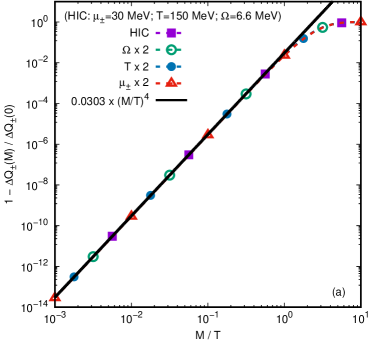
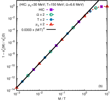
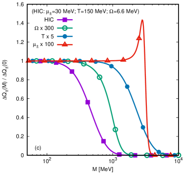
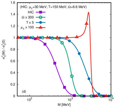
Figure 2: (a-b) Relative mass corrections (a) $1-\Delta Q_{\pm}(M)/\Delta Q_{\pm}(0)$ and (b) $1-\sigma^{\tau}_{\pm}(M)/\sigma^{\tau}_{\pm}(0)$, represented with respect to $M$, for various values of $\Omega$, $T$ and $\mu_{\pm}$. The black curves represent the best fit of the function $\alpha(M/T)^{4}$ to the numerical data ($\alpha\simeq 0.0303$ in both cases). (c-d) Ratios (c) $\Delta Q_{\pm}(M)/\Delta Q_{\pm}(0)$ and (d) $\sigma^{\tau}_{\pm}(M)/\sigma^{\tau}_{\pm}(0)$, represented with respect to $M$, for various values of $\Omega$, $T$ and $\mu_{\pm}$. The set of parameters indicated at the top of each image corresponds to the values typical of Heavy Ion Collisions (HIC) and the corresponding data set is represented using the purple curve and filled squares. For each subsequent curve, only the parameter indicated in the legend is changed, compared to the HIC set.

The discussion in this section begins by considering the behaviour of the correction $\Delta Q_{\pm}$ to the charge density and the circular conductivity $\sigma_{\pm}^{\tau}$ as the mass is increased. The analysis in the previous subsection showed that there are no contributions to $\Delta Q_{\pm}$ and $\sigma^{\tau}_{\pm}$ from the mass term up to $O(M^{4})$. Figures 2(a) and 2(b) validate this prediction by considering the dependence of the relative mass corrections, $1-\Delta Q_{\pm}(M)/\Delta Q_{\pm}(0)$ and $1-\sigma^{\tau}_{\pm}(M)/\sigma^{\tau}_{\pm}(0)$, with respect to $M/T$. It can be seen that, close to the parameters relevant to heavy ion collisions (labelled HIC and shown with dashed purple lines and squares), the relative mass corrections have a universal behaviour of the type $\alpha(M/T)^{4}$, where $\alpha\simeq 0.0303$ gives the best fit of this power law to the numerical data. Figures 2(c) and 2(d) show the ratios $\Delta Q_{\pm}(M)/\Delta Q_{\pm}(0)$ and $\sigma^{\tau}_{\pm}(M)/\sigma^{\tau}_{\pm}(0)$ with respect to $M$. The massless limits $\Delta Q_{\pm}(0)$ and $\sigma_{\pm}^{\tau}(0)$ are taken from Eq. (141), while $\Delta Q_{\pm}(M)$ and $\sigma^{\tau}_{\pm}(M)$ are obtained by directly integrating Eq. (119). For the HIC parameters, it can be seen that the constitutive relations derived in Eq. (141) are valid for $M\lesssim T=150\ {\rm MeV}$. Increasing the mass has the expected effect of suppressing the t.e.v.s with respect to their values obtained in the massless case. To further test the robustness of the constitutive equations, three more curves are represented. For each curve, only one parameter from the original list is increased. This parameter is indicated in the legend, together with the corresponding multiplier. The second curve (green and empty circles), corresponding to $\Omega\simeq 2\ {\rm GeV}$, shows that the validity domain of Eq. (141) is enhanced at higher values of $\Omega$, with deviations occurring at $M\gtrsim\Omega/4$. The third curve (blue and filled circles) shows deviations from the massless prediction also when $M\gtrsim T=750\ {\rm MeV}$. Finally, the last curve (red line and empty triangles) curresponds to $\mu_{\pm}=3\ {\rm GeV}\gg T=150\ {\rm MeV}$. In this case, the fermion fluid is strongly degenerate, such that a strong suppression can be seen when $M$ exceeds $\mu_{\pm}$. Also, for $Mc^{2}<\mu_{\pm}$, the constitutive relations for the massless case retain their validity, except in the vicinity $M\simeq\mu_{\pm}$. Here, a strong deviation can be seen, indicating an unexpected resonance. While this regime does not seem to be of immediate relevance to the field of relativistic heavy ion collisions, it is worth exploring its origin.

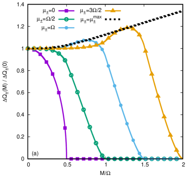
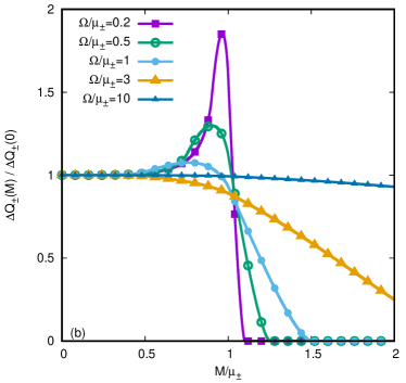
Figure 3: Ratio $\Delta Q_{\pm}(M)/\Delta Q_{\pm}(0)$ at vanishing temperature represented with respect to (a) $M/\Omega$ at fixed $\Omega$, for various values of $\mu_{\pm}/\Omega$; and (b) $M/\mu_{\pm}$ at fixed $\mu_{\pm}$, for various values of $\Omega/\mu_{\pm}$.

The starting point for the analysis of the vanishing temperature regime is to take the $\beta_{0}\rightarrow\infty$ limit of Eq. (119). Restricting the analysis to the axis of rotation, the following result is obtained for the quantum correction to the charge density:

$$\Delta Q_{\pm}\rfloor_{T\rightarrow 0}=\frac{{\rm sgn}(\mu_{\pm})}{6\pi^{2}}\left\{\left[\left(|\mu_{\pm}|+\frac{|\Omega|}{2}\right)^{2}-M^{2}\right]^{3/2}\theta\left(|\mu_{\pm}|+\frac{|\Omega|}{2}-M\right)\right.\\ +\left[\left(|\mu_{\pm}|-\frac{|\Omega|}{2}\right)^{2}-M^{2}\right]^{3/2}\left[\theta\left(|\mu_{\pm}|-\frac{|\Omega|}{2}-M\right)-\theta\left(\frac{|\Omega|}{2}-|\mu_{\pm}|-M\right)\right]\\ \left.-2(\mu_{\pm}^{2}-M^{2})^{3/2}\theta(|\mu_{\pm}|-M)\right\},$$ (143)

where the last line corresponds to the RKT contribution $Q^{\rm RKT}_{\pm}$, which can be obtained by taking the vanishing temperature limit of Eq. (56):

$$Q^{\rm RKT}_{\pm}\rfloor_{T\rightarrow 0}=\frac{{\rm sgn}(\mu_{\pm})}{3\pi^{2}}(\mu_{\pm}^{2}-M^{2})^{3/2}\theta(|\mu_{\pm}|-M).$$ (144)

When $|\mu_{\pm}|-\frac{|\Omega|}{2}<M<|\mu_{\pm}|$ and the term on the second line in Eq. (143) cancels, $\Delta Q_{\pm}$ admits an extremum with respect to $M$, which is obtained by solving $d\Delta Q_{\pm}/dM=0$:

$$M_{\rm max}= \sqrt{\left(|\mu_{\pm}|+\frac{|\Omega|}{6}\right)\left(|\mu_{\pm}|-\frac{|\Omega|}{2}\right)},$$

$$\Delta Q_{\pm}(M_{\rm max})= \frac{\mu_{\pm}^{3}}{3\pi^{2}\sqrt{3}}\left[\left(1+\frac{|\Omega|}{2|\mu_{\pm}|}\right)^{2}-1\right]^{3/2}.$$ (145)

It is understood that this maximum occurs only when $|\mu_{\pm}|>|\Omega|/2$. This behaviour is confirmed in Fig. 3(a), where the ratio $\Delta Q_{\pm}(M)/\Delta Q_{\pm}(0)$ is represented at fixed $\Omega$ with respect to the ratio $M/\Omega$, for various values of $\mu_{\pm}$. The dotted black line represents the value of this ratio when $|\mu_{\pm}|=\mu_{\pm}^{\rm max}$, where

$$\mu_{\pm}^{\rm max}=\frac{|\Omega|}{6}+\sqrt{M^{2}+\frac{\Omega^{2}}{9}}.$$ (146)

When $|\Omega/\mu_{\pm}|\ll 1$ and $M_{\rm max}\rightarrow|\mu_{\pm}|$, $\Delta Q_{\pm}(M_{\rm max})/\Delta Q_{\pm}(0)$ peaks sharply around $M=M_{\rm max}$:

$$\frac{\Delta Q_{\pm}(M_{\rm max})}{\Delta Q_{\pm}(0)}\simeq\frac{4}{3}\sqrt{\frac{|\mu_{\pm}|}{3|\Omega|}}+O(|\Omega/\mu_{\pm}|^{1/2}).$$ (147)

The development of this peak is highlighted in Fig. 3(b). For the case considered in Fig. 2(c), the ratio between the chemical potential and the rotation parameter is $\mu_{\pm}/\Omega\simeq 450$. In this case, Eq. (147) predicts that $\Delta Q_{\pm}(M_{\rm max})/\Delta Q_{\pm}(0)\simeq 16.4$, compared to $\simeq 1.5$ observed in Fig. 2(c). This discrepancy is an indication of the thermal suppression of this effect, which is already significant for the values in Fig. 2(c), when $T_{0}/\mu_{\pm}=0.05$.

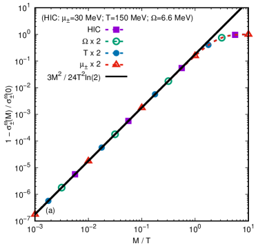
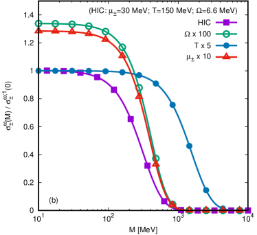
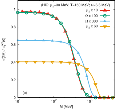
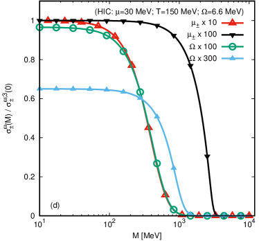
Figure 4: (a) Relative mass correction $1-\sigma^{\omega}_{\pm}(M)/\sigma^{\omega}_{\pm}(0)$, with both $\sigma^{\omega}_{\pm}(M)$ and $\sigma^{\omega}_{\pm}(0)$ computed from Eq. (138), represented with respect to $M/T$ with dotted lines and symbols. The solid black line represents the analytic prediction $3M^{2}/24T^{2}\ln(2)$, derived from Eqs. (133) and (140). (b)–(d) Ratio $\sigma^{\omega}_{\pm}(M)/\sigma^{\omega;n}_{\pm}(0)$, evaluated on the rotation axis, with $\sigma^{\omega}_{\pm}(M)$ computed using Eq. (138) and the approximations $\sigma^{\omega;n}_{\pm}(0)$ are given for (b) $n=1$, (c) $n=2$ and (d) $n=3$ in Eqs. (148), (149) and (150), respectively.

The validity of the results derived for the vortical charge current conductivity $\sigma^{\omega}_{\pm}$ is now considered. An exact result was obtained in Eq. (138) for this quantity evaluated on the rotation axis, which is valid at any mass. Figure 4(a) shows that, in the vicinity of the HIC parameters, the relative mass correction $1-\sigma^{\omega}(M)/\sigma^{\omega}(0)$ is well represented by the quadratic term $3M^{2}/24T^{2}\ln(2)$ highlighted in Eqs. (133) and (140).

Away from the rotation axis, the result for $\sigma^{\omega}_{\pm}$ was obtained only up to O($\Omega^{4}$) in Eq. (131). This expression, involving the polylogarithm function, is approximate even on the rotation axis. To test its validity for relativistic heavy ion collisions, various levels of approximation $\sigma^{\omega;n}_{\pm}$ are considered based on Eq. (131), distinguished using the index $n$. The $n=1$ approximation corresponds to the leading order with respect to the temperature, highlighted in Eq. (133) and reproduced below:

$$\sigma^{\omega;1}_{\pm}=\pm\frac{2\mu_{\pm}T}{\pi^{2}}\ln 2.$$ (148)

As can be seen from Fig. 4(b), $\sigma^{\omega;1}_{\pm}$ offers a very good approximation under the HIC conditions. The mass corrections are important only when $M\gtrsim T$, even for $T=750\ {\rm MeV}$. However, when $\mu_{\pm}$ or $\Omega$ become comparable with $T$, deviations can be seen. In order to understand the nature of these deviations, the next to leading order is considered below, which can also be read from Eq. (133):

$$\sigma^{\omega;2}_{\pm}=\pm\frac{2\mu_{\pm}T}{\pi^{2}}\ln 2\pm\frac{\mu_{\pm}}{12\pi^{2}T}\left[\mu_{\pm}^{2}+\frac{\bm{\omega}^{2}+3\bm{a}^{2}}{4}\right].$$ (149)

In the above, the mass contribution was not taken into account. As can be seen from Fig. 4(c), this approximation improves the small $M$ results at moderate values for $\Omega$ and $\mu_{\pm}$. However, increasing $\mu_{\pm}$ and $\Omega$ further brings about new discrepancies. The final approximation, $\sigma^{\omega;3}_{\pm}$, corresponds to the result in Eq. (131), written without the mass term:

$$\sigma^{\omega;3}_{\pm}=\pm\frac{T^{2}}{\pi^{2}}\left[{\rm Li}_{2}(-e^{-\mu_{\pm}/T})-{\rm Li}_{2}(-e^{\mu_{\pm}/T})\right]\pm\frac{\bm{\omega}^{2}+3\bm{a}^{2}}{24\pi^{2}}\tanh\frac{\mu_{\pm}}{2T}.$$ (150)

Figure 4(d) shows that the above approximation correctly accounts for the chemical potential, even when $\mu_{\pm}/T\gg 1$. However, no improvement can be seen for the case of large values of $\Omega$, which is to be expected since Eq. (131) was obtained following a truncation at order $O(\Omega^{4})$.

7 Axial current

Initially shown to be so by Vilenkin vilenkin78 , it is known that the local vorticity induces an axial current parallel to the vorticity vector through the chiral vortical effect kharzeev16 . This section presents an analysis of the effect of helicity imbalance induced by the helicity chemical potential $\mu_{H}$ on the thermal expectation value (t.e.v.) of the axial charge current (ACC) operator $\widehat{J}_{A}^{\hat{\alpha}}$, introduced in Eq. (32). The analysis begins with a general discussion of the t.e.v. of the ACC, presented in Subsec. 7.1, followed by analytical and numerical analyses of the finite mass regime in Subsecs. 7.2 and 7.3.

7.1 General analysis

The bilinear form introduced in Eq. (87) corresponding to the ACC, defined in Eq. (32), is

$$\mathcal{J}^{\hat{\alpha}}_{A}(\psi,\chi)=\overline{\psi}\gamma^{\hat{\alpha}}\gamma^{5}\chi.$$ (151)

Noting that $\mathcal{J}^{\hat{\alpha}}_{A}(V_{j},V_{j})=-[\mathcal{J}^{\hat{\alpha}}_{A}(U_{j},U_{j})]^{*}=-\mathcal{J}^{\hat{\alpha}}_{A}(U_{j},U_{j})$, it can be seen that the second line in Eq. (101) does not contribute to the t.e.v. $\braket{:J^{\hat{\alpha}}_{A}:_{\Omega}}$, however, there will be an extra vacuum contribution to the t.e.v. computed with respect to the Minkowski vacuum, $\braket{:J^{\hat{\alpha}}_{A}:_{M}}$. Using the following relations:

$$\mathcal{J}^{\hat{t}}_{A}(U_{j},U_{j})= \frac{p_{j}}{8\pi^{2}E_{j}}\left[2\lambda_{j}J_{m_{j}}^{+}(q_{j}\rho)+\frac{k_{j}}{p_{j}}J_{m_{j}}^{-}(q_{j}\rho)\right],$$

$$\mathcal{J}^{\hat{\varphi}}_{A}(U_{j},U_{j})= \frac{\lambda_{j}q_{j}}{4\pi^{2}p_{j}}J_{m_{j}}^{\times}(q_{j}\rho),$$

$$\mathcal{J}^{\hat{z}}_{A}(U_{j},U_{j})= \frac{1}{8\pi^{2}}\left[J_{m_{j}}^{-}(q_{j}\rho)+\frac{2\lambda_{j}k_{j}}{p_{j}}J_{m_{j}}^{+}(q_{j}\rho)\right],$$ (152)

the t.e.v.s of the components of the ACC taken with respect to the rotating vacuum can be written as follows:

$$\begin{pmatrix}\braket{:\widehat{J}^{{\hat{t}}}_{A}:_{\Omega}}\\ \braket{:\widehat{J}^{{\hat{\varphi}}}_{A}:_{\Omega}}\\ \braket{:\widehat{J}^{{\hat{z}}}_{A}:_{\Omega}}\end{pmatrix}=\frac{1}{4\pi^{2}}\sum_{\lambda=\pm\frac{1}{2}}\sum_{m=-\infty}^{\infty}\int_{M}^{\infty}dE\,{\rm sgn}(\widetilde{E})\\ \times\left[\frac{1}{e^{\beta_{0}(|\widetilde{E}|-\mu_{\lambda;0})}+1}+\frac{1}{e^{\beta_{0}(|\widetilde{E}|+\mu_{\lambda;0})}+1}\right]\int_{0}^{p}dk\begin{pmatrix}2\lambda p\,J_{m}^{+}(q\rho)\\ 2\lambda\frac{qE}{p}J_{m}^{\times}(q\rho)\\ E\,J_{m}^{-}(q\rho)\end{pmatrix}.$$ (153)

The t.e.v.s expressed with respect to the Minkowski vacuum are:

$$\begin{pmatrix}\braket{:\widehat{J}^{{\hat{t}}}_{A}:_{M}}\\ \braket{:\widehat{J}^{{\hat{\varphi}}}_{A}:_{M}}\\ \braket{:\widehat{J}^{{\hat{z}}}_{A}:_{M}}\end{pmatrix}=\frac{1}{4\pi^{2}}\sum_{\lambda=\pm\frac{1}{2}}\sum_{m=-\infty}^{\infty}\int_{M}^{\infty}dE\\ \times\left[\frac{1}{e^{\beta_{0}(\widetilde{E}-\mu_{\lambda;0})}+1}+\frac{1}{e^{\beta_{0}(\widetilde{E}+\mu_{\lambda;0})}+1}\right]\int_{0}^{p}dk\begin{pmatrix}2\lambda p\,J_{m}^{+}(q\rho)\\ 2\lambda\frac{qE}{p}J_{m}^{\times}(q\rho)\\ E\,J_{m}^{-}(q\rho)\end{pmatrix}.$$ (154)

Due to the factors of $2\lambda$ in $\braket{:\widehat{J}^{{\hat{t}}}_{A}:_{M}}$ and $\braket{:\widehat{J}^{{\hat{\varphi}}}_{A}:_{M}}$, it is clear that these components vanish when $\mu_{H;0}=0$. Thus, the t.e.v.s of these two components computed with respect to the Minkowski and rotating vacua coincide, i.e.

$$\braket{:\widehat{J}^{{\hat{t}}}_{A}:_{M}}=\braket{:\widehat{J}^{{\hat{t}}}_{A}:_{\Omega}},\qquad\braket{:\widehat{J}^{{\hat{\varphi}}}_{A}:_{M}}=\braket{:\widehat{J}^{{\hat{\varphi}}}_{A}:_{\Omega}}.$$ (155)

As was the case for the VCC and HCC, the t.e.v. of the ACC can be decomposed as:

$$\braket{:\widehat{J}^{\hat{\alpha}}_{A}:_{\Omega}}=Q_{A}u^{\hat{\alpha}}+\mathcal{J}_{A}^{\hat{\alpha}},\qquad\mathcal{J}_{A}^{\hat{\alpha}}=\sigma_{A}^{\tau}\tau^{\hat{\alpha}}+\sigma_{A}^{\omega}\omega^{\hat{\alpha}}.$$ (156)

7.2 Small mass limit

The t.e.v.s of the components of the ACC taken with respect to the Minkowski vacuum can be put in the form:

$$\begin{pmatrix}\braket{:\widehat{J}^{\hat{t}}_{A}:_{M}}\\ \braket{:\widehat{J}^{\hat{\varphi}}_{A}:_{M}}\\ \braket{:\widehat{J}^{\hat{z}}_{A}:_{M}}\end{pmatrix}=\frac{1}{2\pi^{2}}\sum_{\lambda=\pm\frac{1}{2}}\sum_{j=0}^{\infty}(\rho\Omega)^{2j}\sum_{n=0}^{\infty}\frac{\Omega^{2n}s_{n+j,j}^{+}}{(2n+2j+1)!}\int_{M}^{\infty}dE\,p^{2j}\\ \times\frac{d^{2n+2j}}{dE^{2n+2j}}\left[\frac{1}{e^{\beta_{0}(E-\mu_{\lambda,0})}+1}+\frac{1}{e^{\beta_{0}(E+\mu_{\lambda,0})}+1}\right]\begin{pmatrix}{\displaystyle\frac{2n+2j+1}{2j+1}2\lambda p^{2}}\\ {\displaystyle\frac{2\lambda\rho\Omega}{2j+3}[p^{2}+(2j+2)E^{2}]}\\ {\displaystyle\frac{\Omega}{2p}[p^{2}+(2j+1)E^{2}]}\end{pmatrix}.$$ (157)

For the $z$ component of the t.e.v. of the AC, the small mass limit can be derived in closed form. After changing the integration variable to $dp=\frac{E}{p}dE$, the procedure introduced in Eq. (104) can be used to obtain:

$$\braket{:\widehat{J}^{\hat{z}}_{A}:_{M}}=\frac{\Omega}{4\pi^{2}}\sum_{\lambda=\pm\frac{1}{2}}\sum_{j=0}^{\infty}(\rho\Omega)^{2j}\sum_{n=0}^{\infty}\frac{\Omega^{2n}s_{n+j,j}^{+}}{(2n+2j+1)!}\int_{0}^{\infty}dp\left[(2j+2)p^{2j+1}-j(2j+1)M^{2}p^{2j-1}\right]\\ \times\frac{d^{2n+2j}}{dp^{2n+2j}}\left[\frac{1}{e^{\beta_{0}(E-\mu_{\lambda,0})}+1}+\frac{1}{e^{\beta_{0}(E+\mu_{\lambda,0})}+1}\right],$$ (158)

where the coefficient of $M^{2}$ was obtained after noting that $E\simeq p+\frac{M^{2}}{2p}$ and $\frac{1}{E}\simeq\frac{1}{p}-\frac{M^{2}}{2p^{3}}$. In the term proportional to $M$, the $j=0$ term is infrared divergent and must be treated separately. After performing integration by parts $2j$ times, the following formula can be used for the integration with respect to $p$:

$$\int_{0}^{\infty}dp\,p\frac{d^{2n}}{dp^{2n}}\left[\frac{1}{e^{\beta_{0}(E-\mu_{\lambda,0})}+1}+\frac{1}{e^{\beta_{0}(E+\mu_{\lambda,0})}+1}\right]=\begin{cases}2I_{0}^{+}(\beta\mu_{\lambda})/\beta_{0}^{2},&n=0,\\ 1,&n=1,\\ 0,&n>1,\end{cases}$$ (159)

where $I_{0}^{+}(a)$ is given in Eq. (237). It is not difficult to see that the sum over $n$ terminates at $n=1$ for the first term and at $n=0$ for the second term. The exact result is:

$$\braket{:\widehat{J}^{\hat{z}}_{A}:_{M}}= \left[\sigma_{A}^{\omega}+\frac{\bm{\omega}^{2}+3\bm{a}^{2}}{24\pi^{2}}-\frac{M^{2}}{4\pi^{2}}+O(M^{4})\right]\omega^{\hat{z}},$$

$$\sigma_{A}^{\omega}= \frac{T^{2}}{6}+\frac{\mu_{V}^{2}+\mu_{H}^{2}}{2\pi^{2}}+O(M^{4}),$$ (160)

where $a=-\rho\Omega^{2}\Gamma^{2}e_{\hat{\rho}}$ and $\omega=\Omega\Gamma^{2}e_{\hat{z}}$ are the acceleration and vorticity vectors, introduced in Eqs. (9) and (11), respectively, while their squares $\bm{\omega}^{2}=-\omega^{2}\geq 0$ and $\bm{a}^{2}=-a^{2}\geq 0$ are given in Eq. (13). The second and third terms inside the square brackets in Eq. (160) are purely vacuum contributions which are not taken into account in the definition of $\sigma_{A}^{\omega}$.

It is worth comparing the result in Eq. (160) with the one obtained in Ref. prokhorov18 using the Wigner function proposed in Ref. becattini13 :

$$\braket{j^{5}_{\mu}}=\left(\frac{1}{6}\left[T^{2}+\frac{a^{2}-\omega^{2}}{4\pi^{2}}\right]+\frac{\mu^{2}}{2\pi^{2}}\right)\omega_{\mu}.$$ (161)

Noting that $\omega^{2}=-\bm{\omega}^{2}$ and $a^{2}=-\bm{a}^{2}$, it can be seen that the parts which depend on $T$ and $\mu=\mu_{V}$ reproduced in Eq. (161) agree with those obtained in Eq. (160), when $\mu_{H}=0$. There is a discrepancy in the vacuum term, equal to

$$\braket{:\widehat{J}^{\hat{z}}_{A}:_{M}}-\braket{j_{5}^{z}}=\frac{\bm{a}^{2}}{6\pi^{2}}\omega^{\hat{z}},$$ (162)

which may be due to a fundamental difference between the formulation based on the Wigner function (employed in Ref. prokhorov18 ) and the QFT formulation employed in this work.

As opposed to the case of the ${\hat{z}}$ component, the sum over $n$ in Eq. (157) no longer terminates when considering the ${\hat{t}}$ and ${\hat{\varphi}}$ components, which is an indication that their dependence on $\Gamma$ and $\Omega$ is non-polynomial (see also the discussion in Subsec. 6.2). Performing the change of integration variable from $E$ to $p$ ($dp=EdE/p$) in Eq. (157) and using Eq. (106) gives:

$$\braket{:\widehat{J}^{\hat{t}}_{A}:_{\Omega}}= \frac{1}{4\pi^{2}}\sum_{\lambda=\pm\frac{1}{2}}2\lambda\sum_{j=0}^{\infty}(\rho\Omega)^{2j}\sum_{n=0}^{\infty}\frac{\Omega^{2n}(2j)!(2j+2)}{(2n+2j)!}s_{n+j,j}^{+}\int_{0}^{\infty}dp\,\left(p^{2}-\frac{M^{2}}{2j+1}\right)$$

$$\qquad\qquad\times\frac{d^{2n}}{dp^{2n}}\left[\frac{1}{e^{\beta_{0}(p-\mu_{\lambda,0})}+1}+\frac{1}{e^{\beta_{0}(p+\mu_{\lambda,0})}+1}\right],$$

$$\braket{:\widehat{J}^{\hat{\varphi}}_{A}:_{\Omega}}= \frac{\rho\Omega}{4\pi^{2}}\sum_{\lambda=\pm\frac{1}{2}}2\lambda\sum_{j=0}^{\infty}(\rho\Omega)^{2j}\sum_{n=0}^{\infty}\frac{\Omega^{2n}(2j+2)!}{(2n+2j+1)!}s_{n+j,j}^{+}\int_{0}^{\infty}dp\,\left(p^{2}-\frac{M^{2}}{2j+3}\right)$$

$$\qquad\qquad\times\frac{d^{2n}}{dp^{2n}}\left[\frac{1}{e^{\beta_{0}(p-\mu_{\lambda,0})}+1}+\frac{1}{e^{\beta_{0}(p+\mu_{\lambda,0})}+1}\right].$$ (163)

Taking into account the $n=0$ and $n=1$ terms gives:

$$\braket{:\widehat{J}^{\hat{t}}_{A}:_{\Omega}}= \frac{\Gamma}{4\pi^{2}}\sum_{\lambda=\pm\frac{1}{2}}2\lambda\left\{\frac{4}{\beta^{3}}I_{1/2}^{+}(\beta\mu_{\lambda})+\frac{\Omega^{2}\Gamma^{2}(4\Gamma^{2}-1)}{3\beta}I_{-1/2}^{+}(\beta\mu_{\lambda})\right.$$

$$\left.-\frac{2M^{2}}{\beta}\left[1+\frac{{\rm arcsinh}(\rho\Omega\Gamma)}{\rho\Omega\Gamma^{2}}\right]I_{-1/2}^{+}(\beta\mu_{\lambda})+O(\Omega^{4},M^{4},\Omega^{2}M^{2})\right\},$$

$$\braket{:\widehat{J}^{\hat{\varphi}}_{A}:_{\Omega}}= \frac{\rho\Omega\Gamma}{4\pi^{2}}\sum_{\lambda=\pm\frac{1}{2}}2\lambda\left\{\frac{4}{\beta^{3}}I_{1/2}^{+}(\beta\mu_{\lambda})+\frac{\Omega^{2}\Gamma^{2}(4\Gamma^{2}-3)}{3\beta}I_{-1/2}^{+}(\beta\mu_{\lambda})\right.$$

$$\left.-\frac{2M^{2}}{\beta\rho^{2}\Omega^{2}}\left[1-\frac{{\rm arcsinh}(\rho\Omega\Gamma)}{\rho\Omega\Gamma^{2}}\right]I_{-1/2}^{+}(\beta\mu_{\lambda})+O(\Omega^{4},M^{4},\Omega^{2}M^{2})\right\}.$$ (164)

The charge $Q_{A}$ and the circular conductivity $\sigma_{A}^{\tau}$ are

$$Q_{A}= \frac{T^{3}}{\pi^{2}}\sum_{\lambda=\pm\frac{1}{2}}2\lambda I_{1/2}^{+}\left(\frac{\mu_{\lambda}}{T}\right)+\frac{T}{\pi^{2}}\left[\frac{\bm{\omega}^{2}+\bm{a}^{2}}{4}-M^{2}\frac{{\rm arcsinh}(\rho\Omega\Gamma)}{\rho\Omega}\right]\sum_{\lambda=\pm\frac{1}{2}}2\lambda I_{-1/2}^{+}\left(\frac{\mu_{\lambda}}{T}\right)$$

$$+O(\Omega^{4},M^{4},\Omega^{2}M^{2}),$$

$$\sigma_{A}^{\tau}= \frac{T}{6\pi^{2}}\left\{1-\frac{3M^{2}/\Omega^{2}}{\Gamma^{2}(\Gamma^{2}-1)}\left[(2\Gamma^{2}-1)\frac{{\rm arcsinh}(\rho\Omega\Gamma)}{\rho\Omega\Gamma^{2}}-1\right]\right\}\sum_{\lambda=\pm\frac{1}{2}}2\lambda I_{-1/2}^{+}\left(\frac{\mu_{\lambda}}{T}\right)$$

$$+O(\Omega^{4},M^{4},\Omega^{2}M^{2}).$$ (165)

The sum over $\lambda$ can be performed by taking into account the expressions for $I_{\pm 1/2}^{+}$ given in Eq. (246):

$$Q_{A}= \frac{\mu_{H}}{3}\left(T^{2}+\frac{\mu_{H}^{2}+3\mu_{V}^{2}}{\pi^{2}}\right)-\frac{2T^{3}}{\pi^{2}}\left[{\rm Li}_{3}(-e^{-\mu_{+}/T})-{\rm Li}_{3}(-e^{-\mu_{-}/T})\right]$$

$$+\frac{T}{\pi^{2}}\left[\frac{\bm{\omega}^{2}+\bm{a}^{2}}{4}-\frac{M^{2}}{\rho\Omega}{\rm arcsinh}(\rho\Omega\Gamma)\right]\ln\left[\frac{\cosh(\mu_{+}/2T)}{\cosh(\mu_{-}/2T)}\right]+O(\Omega^{4},M^{4},\Omega^{2}M^{2}),$$

$$\sigma_{A}^{\tau}= \frac{T}{6\pi^{2}}\left\{1-\frac{3M^{2}/\Omega^{2}}{\Gamma^{2}(\Gamma^{2}-1)}\left[(2\Gamma^{2}-1)\frac{{\rm arcsinh}(\rho\Omega\Gamma)}{\rho\Omega\Gamma^{2}}-1\right]\right\}\ln\left[\frac{\cosh(\mu_{+}/2T)}{\cosh(\mu_{-}/2T)}\right]$$

$$+O(\Omega^{4},M^{4},\Omega^{2}M^{2}).$$ (166)

The high temperature limit of the above expressions is:

$$Q_{A}= \frac{4\mu_{V}\mu_{H}T}{\pi^{2}}\ln 2+\frac{\mu_{V}\mu_{H}}{2\pi^{2}T}\left[\frac{\mu_{V}^{2}+\mu_{H}^{2}}{3}+\frac{\bm{\omega}^{2}+\bm{a}^{2}}{4}-\frac{M^{2}}{\rho\Omega}{\rm arcsinh}(\rho\Omega\Gamma)\right]+O(T^{-2}),$$

$$\sigma_{A}^{\tau}= \frac{\mu_{V}\mu_{H}}{12\pi^{2}T}\left\{1-\frac{3M^{2}/\Omega^{2}}{\Gamma^{2}(\Gamma^{2}-1)}\left[(2\Gamma^{2}-1)\frac{{\rm arcsinh}(\rho\Omega\Gamma)}{\rho\Omega\Gamma^{2}}-1\right]\right\}+O(T^{-2}).$$ (167)

It can be seen that the mass term makes a significant contribution to $\sigma^{\tau}_{A}$ when $\Omega$ is sufficiently small. This is an indication that the finite mass correction to $\sigma_{A}^{\tau}$ behaves formally different from $\sigma_{A}^{\tau}(M=0)$. Indeed, multiplying $\delta\sigma_{A}^{\tau}=\sigma_{A}^{\tau}(M)-\sigma_{A}^{\tau}(0)$ by the circular vector $\tau^{\hat{\alpha}}$ gives:

$$\delta\sigma_{A}^{\tau}\,\tau= \frac{\mu_{V}\mu_{H}M^{2}\Gamma}{4\pi^{2}T\rho\Omega}\left[\frac{{\rm arcsinh}(\rho\Omega\Gamma)}{\rho\Omega}-1+\rho\Omega{\rm arcsinh}(\rho\Omega\Gamma)\right](\rho\Omega e_{\hat{t}}+e_{\hat{\varphi}})$$

$$\simeq \frac{\mu_{V}\mu_{H}M^{2}}{3\pi^{2}T}[u^{\hat{\varphi}}e_{\hat{\varphi}}+O(\rho^{2}\Omega^{2})],$$ (168)

where $u^{\hat{\varphi}}=\rho\Omega\Gamma$, indicating that $\delta\sigma_{A}^{\tau}\tau^{\hat{\varphi}}$ contributes to $\braket{:J^{\hat{\varphi}}_{A}:_{\Omega}}$ on the same footing as $Q_{A}u^{\hat{\varphi}}$.

The results in Eq. (166) are valid only at small values of $\Omega$. It is possible to obtain exact expressions for $Q_{A}$ and $\sigma^{\tau}_{A}$ on the rotation axis, where

$$Q_{A}\rfloor_{\rho=0}=\braket{:\widehat{J}_{A}^{\hat{t}}:_{\Omega}}\rfloor_{\rho=0},\qquad\sigma_{A}^{\tau}=\left(\braket{:\widehat{J}_{A}^{\hat{t}}:_{\Omega}}-\frac{\braket{:\widehat{J}_{A}^{\hat{\varphi}}:_{\Omega}}}{\rho\Omega^{3}}\right)_{\rho=0}.$$ (169)

Noting that

$$\lim_{\rho\rightarrow 0}J_{m}^{+}(q\rho)=\begin{cases}1,&m=\pm\frac{1}{2},\\ 0,&\text{otherwise},\end{cases}\qquad\lim_{\rho\rightarrow 0}\frac{J_{m}^{\times}(q\rho)}{q\rho}=\begin{cases}\pm 1,&m=\pm\frac{1}{2},\\ 0,&\text{otherwise},\end{cases}$$ (170)

it is not difficult to obtain the following expressions:

$$\braket{:\widehat{J}^{\hat{t}}_{A}:_{\Omega}}= \frac{2M^{3}}{\pi^{2}}\sum_{\ell=1}^{\infty}(-1)^{\ell+1}\cosh\frac{\ell\beta\Omega}{2}\sinh(\ell\beta\mu_{V})\sinh(\ell\beta\mu_{H})\int_{1}^{\infty}dx(x^{2}-1)e^{-\ell\beta xM},$$

$$\frac{\braket{:\widehat{J}^{\hat{\varphi}}_{A}:_{\Omega}}}{\rho\Omega}= \frac{4M^{4}}{3\pi^{2}\Omega}\sum_{\ell=1}^{\infty}(-1)^{\ell+1}\sinh\frac{\ell\beta\Omega}{2}\sinh(\ell\beta\mu_{V})\sinh(\ell\beta\mu_{H})\int_{1}^{\infty}dx\,x(x^{2}-1)e^{-\ell\beta xM},$$ (171)

where $x=E/M$ and Eq. (63) was used to expand the Fermi-Dirac factors. The integration with respect to $x$ can be readily performed and the sums over $\ell$ yield polylogarithm functions. The result can be summarised as:

$$Q_{A}\rfloor_{\rho\rightarrow 0}= -\frac{T^{3}}{2\pi^{2}}\sum_{\sigma_{\Omega}=\pm 1}\sum_{\sigma_{V}=\pm 1}\sigma_{V}\sum_{\sigma_{H}=\pm 1}\sigma_{H}\left[{\rm Li}_{3}(-e^{\zeta})+\frac{M}{T}{\rm Li}_{2}(-e^{\zeta})\right],$$

$$\sigma_{A}^{\tau}\rfloor_{\rho\rightarrow 0}= -\frac{T^{4}}{\pi^{2}\Omega^{3}}\sum_{\sigma_{\Omega}=\pm 1}\sum_{\sigma_{V}=\pm 1}\sigma_{V}\sum_{\sigma_{H}=\pm 1}\sigma_{H}\left\{\frac{\Omega}{2T}\left[{\rm Li}_{3}(-e^{\zeta})+\frac{M}{T}{\rm Li}_{2}(-e^{\zeta})\right]\right.$$

$$\left.-\sigma_{\Omega}\left[{\rm Li}_{4}(-e^{\zeta})+\frac{M}{T}{\rm Li}_{3}(-e^{\zeta})+\frac{M^{2}}{3T^{2}}{\rm Li}_{2}(-e^{\zeta})\right]\right\},$$ (172)

where $\zeta=(\sigma_{\Omega}\frac{\Omega}{2}+\sigma_{V}\mu_{V}+\sigma_{H}\mu_{H}-M)/T$. The above expressions are exact for any particle mass. Extracting the large temperature limit yields:

$$Q_{A}\rfloor_{\rho=0}= \frac{4\mu_{H}\mu_{V}T}{\pi^{2}}\ln 2+\frac{\mu_{H}\mu_{V}}{2\pi^{2}T}\left(\frac{\mu_{H}^{2}+\mu_{V}^{2}}{3}+\frac{\Omega^{2}}{4}-M^{2}\right)+O(T^{-3}),$$

$$\sigma_{A}^{\tau}\rfloor_{\rho=0}= \frac{\mu_{H}\mu_{V}}{12\pi^{2}T}\left(1-\frac{4M^{2}}{\Omega^{2}}\right)+O(T^{-3}).$$ (173)

The above results are in agreement with Eq. (167).

The high temperature limit of the results obtained in this section can be summarised as follows:

$$\braket{:\widehat{J}^{\hat{\alpha}}_{A}:_{\Omega}}= Q_{A}u^{\hat{\alpha}}+\sigma_{A}^{\tau}\tau^{\hat{\alpha}}+\sigma_{A}^{\omega}\omega^{\hat{\alpha}},$$

$$Q_{A}= \frac{4\mu_{V}\mu_{H}T}{\pi^{2}}\ln 2+O(T^{-1}),$$

$$\sigma_{A}^{\tau}= \frac{\mu_{V}\mu_{H}}{12\pi^{2}T}\left(1-\frac{4M^{2}}{\Omega^{2}}\right)+O(T^{-3}),$$

$$\sigma_{A}^{\omega}= \frac{T^{2}}{6}+\frac{\mu_{V}^{2}+\mu_{H}^{2}}{2\pi^{2}}+O(M^{4}).$$ (174)

The mass term was retained in the coefficient of $\tau^{\hat{\alpha}}$ due to its unusual effect. It is worth noting that, in the limit $\mu_{H}=M=0$, the results in Eq. (174) reproduce those reported in Eq. (4.14) and Table 2 of Ref. buzzegoli18 for the case of a vanishing axial chemical pontential ($\mu_{A}=0$).

7.3 Numerical analysis

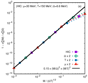
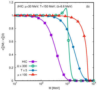
Figure 5: (a) Relative mass correction $1-\sigma^{\omega}_{A}(M)/\sigma^{\omega}_{A}(0)$ and (b) ratio $\sigma^{\omega}_{A}(M)/\sigma^{\omega}_{A}(0)$, evaluated on the rotation axis, where $\sigma^{\omega}_{A}(M)$ is computed numerically using Eq. (153) and $\sigma^{\omega}_{A}(0)$ is taken from Eq. (174). The solid line in (a) represents the best fit of the function $\alpha M^{4}/\Omega^{2}T^{2}$ to the numerical data.

In this section, the validity of the results summarised for the small mass limit in Eq. (174) is investigated as the mass is increased. As mentioned in the introduction, the numerical analysis is focussed on the HIC parameters. In the case of the axial current, the vector and helical chemical potentials play equivalent roles. Thus, for simplicity, the convention $\mu_{V}=\mu_{H}=\mu$ is used throughout this section, which is set to the “HIC” value of $\mu=30\ {\rm MeV}$.

First, the validity of the constitutive equation for $\sigma^{\omega}_{A}$ derived in the small mass limit in Eq. (174) is considered as the mass is increased. At nonvanishing $M$, $\sigma^{\omega}_{A}(M)$ is evaluated numerically starting from Eq. (153). For simplicity, the analysis is limited to the case of the rotation axis. Figure 5(a) confirms that the relative mass correction, $1-\sigma_{A}^{\omega}(M)/\sigma_{A}^{\omega}(0)$, is of fourth order with respect to $M$. Around the HIC parameters, the mass term makes a relative contribution of the form $\alpha M^{4}/\Omega^{2}T^{2}$, where $\alpha\simeq 0.150$ is a dimensionless number. Figure 5(b) presents the ratio $\sigma^{\omega}_{A}(M)/\sigma^{\omega}_{A}(0)$. It can be seen that the constitutive relation holds for $M\lesssim 100\ {\rm MeV}$, which is below the thermal energy ($T=150\ {\rm MeV}$). Increasing the temperature by a factor of $5$ (blue line with filled circles) increases the validity up to $M\simeq 500\ {\rm MeV}$, i.e. by a factor of $5$. At higher chemical potentials ($\mu_{V}=\mu_{H}=\mu=3\ {\rm GeV}$), it can be seen that the constitutive relation remains valid until the mass approaches the Fermi level, which is given by $\sim\mu_{V}+\mu_{H}=6\ {\rm GeV}$. The ratio $\sigma^{\omega}_{A}(M)/\sigma^{\omega}_{A}(0)$ seems to have a monotonic behaviour, as also observed for the ratio $\sigma^{\omega}_{\pm}(M)/\sigma^{\omega}_{\pm}(0)$, shown in Fig. 4. An interesting effect can be observed when the rotation parameter is increased by a factor of $300$, to $\Omega\simeq 2\ {\rm GeV}$. At such a high value, $\Omega/2$ acts like a Fermi level and the maximum observed in Fig. 5 resembles the one highlighted for the ratios $\Delta Q_{\pm}(M)/\Delta Q_{\pm}(0)$ and $\sigma^{\tau}_{\pm}(M)/\sigma^{\tau}_{\pm}(0)$ in Fig. 3. However, in the latter case, the maximum was observed at large chemical potential.

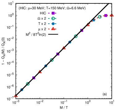
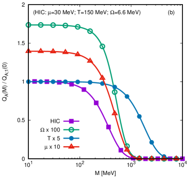
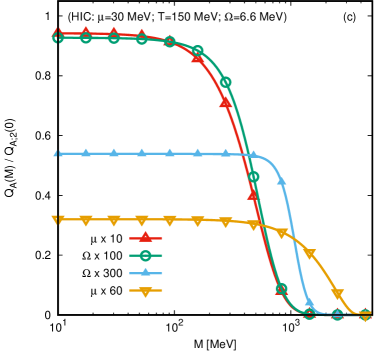
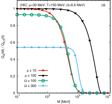
Figure 6: (a) Relative mass correction $1-Q_{A}(M)/Q_{A}(0)$ represented with respect to $M$. The solid black line shows the second order prediction in Eq. (173). (b)-(d) Ratio $Q_{A}(M)/Q_{A;n}(0)$ with respect to $M$, where $Q_{A}(M)$ is computed using Eq. (172), while the approximations $Q_{A;n}(0)$ are given for (b) $n=1$ (c) $n=2$ and (d) $n=3$ in Eqs. (175), (176) and (177), respectively.

Now, the axial charge density $Q_{A}$ and the conductivity $\sigma^{\tau}_{A}$ along $\tau$ are discussed. As opposed to $\sigma^{\omega}_{A}$, it is not possible to obtain the radial profiles of these quantities analytically, even in the massless limit. Instead, Eq. (166) gives $Q_{A}$ and $\sigma_{A}^{\tau}$ up to order $O(\Omega^{4},M^{4},\Omega^{2}M^{2})$ at any distance $\rho$ from the rotation axis, while Eq. (172) gives exact expressions for their values on the rotation axis. The latter expressions involve the polylogarithm function. More insightful expressions can be obtained by considering the high temperature expansions (167) and (173).

In the case of $Q_{A}$, according to Eq. (167), the mass term makes second order contributions of the form $O(M^{2}/T^{2})$. This is confirmed in Fig. 6(a), where the relative mass correction $1-Q_{A}(M)/Q_{A}(0)$ is represented with respect to $M/T$. Both $Q_{A}(M)$ and $Q_{A}(0)$ are evaluated using Eq. (172), which is valid on the rotation axis for any mass. In the vicinity of the HIC parameters, $M^{2}/8T^{2}\ln 2$ provides a good approximation for the relative mass corrections. Away from the rotation axis, Eq. (166) provides an approximation which is obtained using a small $\Omega$ expansion. Eq. (166) involves the polylogarithm function, and is thus less insightful compared to its high temperature expansion presented in Eq. (167). In what follows, three levels of approximation are considered, denoted using $Q_{A;n}$ ($1\leq n\leq 3$), which are based on Eq. (166). Their validity is tested compared with the exact solution in Eq. (172). The first two approximations take into account the leading and next-to-leading order terms in the high temperature expansion, given in Eq. (167):

$$Q_{A;1}= \frac{4\mu_{H}\mu_{V}T}{\pi^{2}}\ln 2,$$ (175)

$$Q_{A;2}= \frac{4\mu_{H}\mu_{V}T}{\pi^{2}}\ln 2+\frac{\mu_{H}\mu_{V}}{2\pi^{2}T}\left(\frac{\mu_{H}^{2}+\mu_{V}^{2}}{3}+\frac{\bm{\omega}^{2}+\bm{a}^{2}}{4}\right).$$ (176)

The third expression is the massless limit of Eq. (166):

$$Q_{A;3}=\frac{\mu_{H}}{3}\left(T^{2}+\frac{\mu_{H}^{2}+3\mu_{V}^{2}}{\pi^{2}}\right)-\frac{2T^{3}}{\pi^{2}}\left[{\rm Li}_{3}(-e^{-\mu_{+}/T})-{\rm Li}_{3}(-e^{-\mu_{-}/T})\right]\\ +\frac{T}{\pi^{2}}\frac{\bm{\omega}^{2}+\bm{a}^{2}}{4}\ln\left[\frac{\cosh(\mu_{+}/2T)}{\cosh(\mu_{-}/2T)}\right].$$ (177)

Figures 6(b), 6(c) and 6(d) show the ratio $Q_{A}(M)/Q_{A;n}(M)$ for $n=1$, $2$ and $3$, respectively. It can be seen in Fig. 6(b) that $Q_{A;1}(0)$ is a good approximation for $Q_{A}$ on the axis in the case of the HIC parameters for $M\lesssim T/3$. This inequality is confirmed also when the temperature is increased by a factor of $5$ (red curve and filled circles). At higher values of the rotation parameter ($\Omega\simeq 660\ {\rm MeV}$) or of the chemical potentials ($\mu_{V}=\mu_{H}=300\ {\rm MeV}$), $Q_{A;1}$ is no longer a good approximation for $Q_{A}(0)$. Panel (c) shows that $Q_{A;2}$ is much better at these values, though it still presents a relative error of about $10\%$. The validity of $Q_{A;2}$ worsens as $\Omega$ and $\mu$ are further increased. Finally, panel (d) shows that considering the polylogarithms in Eq. (177) is sufficient to correctly account for any value of the chemical potential. The agreement between $Q_{A;3}(0)$ and $Q_{A}(0)$ is very good even at $\mu_{V}=\mu_{H}=\mu=3\ {\rm GeV}$. However, the discrepancies at high $\Omega$ persist, since Eq. (172) is valid only up to second order in $\Omega$. For all parameters studied, it seems that the variations with respect to the mass appear only at $M\gtrsim 100\ {\rm MeV}$.

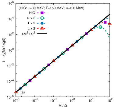
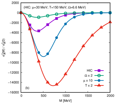
Figure 7: (a) Relative mass correction $1-\sigma^{\tau}_{A}(M)/\sigma^{\tau}_{A}(0)$ and (b) ratio $\sigma^{\tau}_{A}(M)/\sigma^{\tau}_{A}(0)$, where $\sigma^{\tau}_{A}(M)$ and $\sigma^{\tau}_{A}(0)$ are computed using the exact expression in Eq. (172). The solid black line in (a) corresponds to the analytic prediction for the $M^{2}$ correction given in the high temperature expansion of $\sigma^{\tau}_{A}(M)$ in Eq. (173).

Considering now the properties of $\sigma^{\tau}_{A}$, Eq. (167) indicates that it receives corrections due to the mass term which are proportional to $M^{2}/\Omega^{2}$. This is confirmed in Fig. 7(a), which shows the relative mass correction $1-\sigma^{\tau}_{A}(M)/\sigma^{\tau}_{A}(0)$ with respect to the ratio $M/\Omega$. Surprisingly, the analytic prediction $4M^{2}/\Omega^{2}$ is dominant for parameters in the vicinity of the HIC values at high values of $M/\Omega$, where the mass term dominates by a few orders of magnitude over the massless limit. This behaviour is also confirmed in Fig. 7(b), where the ratio $\sigma^{\tau}_{A}(M)/\sigma^{\tau}_{A}(0)$ is shown with respect to $M$. It can be seen that this ratio achieves negative values for the HIC parameters. Furthermore, $|\sigma^{\tau}_{A}(M)|$ increases with respect to the massless prediction $\sigma^{\tau}_{A}(0)$ by a few orders of magnitude as $M$ is increased, decreasing to $0$ after reaching a maximum. The amplitude of this maximum decreases when $\Omega$ is increased, but it increases when either $\mu_{V}=\mu_{H}=\mu$ or $T$ are increased (the two chemical potentials play an equivalent role). Furthermore, the maximum shifts to higher values of $M$ when the chemical potentials or $T$ are increased.

8 Fermion condensate

In this section, the t.e.v. of the fermion condensate (FC), $\frac{1}{2}[\widehat{\overline{\Psi}},\widehat{\Psi}]$, is considered. Subsection 8.1 presents the general expression for the t.e.v. of the FC, while Subsections 8.2 and 8.3 are dedicated to its analytical and numerical analyses.

8.1 General analysis

The bilinear form introduced in Eq. (87) which corresponds to the FC is:

$${\rm FC}(\psi,\chi)=\overline{\psi}\chi.$$ (178)

After noting that $\overline{V}_{j}V_{j}=-(\overline{U}_{j}U_{j})^{*}$, it is easy to see that the term on the second line of Eq. (101) makes a vanishing contribution to the t.e.v. of the FC. Furthermore, the expressions in Eq. (72) for the particle modes allow the following result to be obtained:

$${\rm FC}(U_{j},U_{j})=\frac{M}{8\pi^{2}E_{j}}\left[J_{m_{j}}^{+}(q_{j}\rho)+\frac{2\lambda_{j}k_{j}}{p_{j}}J_{m_{j}}^{-}(q_{j}\rho)\right],$$ (179)

allowing the t.e.v. of the FC to be put in the following form:

$$\braket{:\frac{1}{2}[\widehat{\overline{\Psi}},\widehat{\Psi}]:_{\Omega}}=\frac{M}{4\pi^{2}}\sum_{\lambda=\pm\frac{1}{2}}\sum_{m=-\infty}^{\infty}\int_{M}^{\infty}dE\,{\rm sgn}(\widetilde{E})\\ \times\left[\frac{1}{e^{\beta_{0}(|\widetilde{E}|-\mu_{\lambda;0})}+1}+\frac{1}{e^{\beta_{0}(|\widetilde{E}|+\mu_{\lambda;0})}+1}\right]\int_{0}^{p}dk\,J_{m}^{+}(q\rho).$$ (180)

Taken with respect to the Minkowski vacuum, the t.e.v. of the FC becomes:

$$\braket{:\frac{1}{2}[\widehat{\overline{\Psi}},\widehat{\Psi}]:_{M}}=\frac{M}{4\pi^{2}}\sum_{\lambda=\pm\frac{1}{2}}\sum_{m=-\infty}^{\infty}\int_{M}^{\infty}dE\,\left[\frac{1}{e^{\beta_{0}(\widetilde{E}-\mu_{\lambda;0})}+1}+\frac{1}{e^{\beta_{0}(\widetilde{E}+\mu_{\lambda;0})}+1}\right]\\ \times\int_{0}^{p}dk\,J_{m}^{+}(q\rho),$$ (181)

which differs from the t.e.v. in Eq. (180) by a vacuum term.

8.2 Small mass limit

Employing the same method as in Subsec. 6.2, the t.e.v. of the FC taken with respect to the Minkowski vacuum can be put in the form:

$$\braket{:\frac{1}{2}[\widehat{\overline{\Psi}},\widehat{\Psi}]:_{M}}=\frac{M}{2\pi^{2}}\sum_{\lambda=\pm\frac{1}{2}}\sum_{j=0}^{\infty}\frac{(\rho\Omega)^{2j}}{2j+1}\sum_{n=0}^{\infty}\frac{\Omega^{2n}s_{n+j,j}^{+}}{(2n+2j)!}\int_{0}^{\infty}dp\,\frac{p^{2j+2}}{E}\\ \times\frac{d^{2n+2j}}{dE^{2n+2j}}\left[\frac{1}{e^{\beta_{0}(E-\mu_{\lambda,0})}+1}+\frac{1}{e^{\beta_{0}(E+\mu_{\lambda,0})}+1}\right].$$ (182)

The correction due to the mass cannot be obtained using the methodology from Eq. (106), due to an infrared divergence of the $j=0$ term. Dividing Eq. (182) by $M$ and taking the massless limit leads to:

$$\braket{:\frac{1}{2}[\widehat{\overline{\Psi}},\widehat{\Psi}]:_{M}}=M\left[\frac{T^{2}}{6}+\frac{\mu_{V}^{2}+\mu_{H}^{2}}{2\pi^{2}}+\frac{3\bm{\omega}^{2}-\bm{a}^{2}}{24\pi^{2}}\right]+O(M^{2}),$$ (183)

where $T=T_{0}\Gamma$, $\mu_{V/H}=\mu_{V/h,0}\Gamma$, $\omega=\Omega\Gamma^{2}e_{\hat{z}}$ and $a=\rho\Omega^{2}\Gamma^{2}e_{\hat{\rho}}$, while $\bm{\omega}^{2}=-\omega^{2}$ and $\bm{a}^{2}=-a^{2}$. The last term is the vacuum contribution corresponding to the difference between the t.e.v.s taken with respect to the rotation and Minkowski vacua, respectively. This contribution must be subtracted in order to obtain the t.e.v. of the FC with respect to the rotating vacuum:

$$\braket{:\frac{1}{2}[\widehat{\overline{\Psi}},\widehat{\Psi}]:_{\Omega}}=M\left(\frac{T^{2}}{6}+\frac{\mu_{V}^{2}+\mu_{H}^{2}}{2\pi^{2}}\right)+O(M^{2}).$$ (184)

It is surprising that Eq. (184) coincides with the RKT prediction $(E_{\rm RKT}-3P_{\rm RKT})/M$ given in Eq. (57).

8.3 Numerical analysis

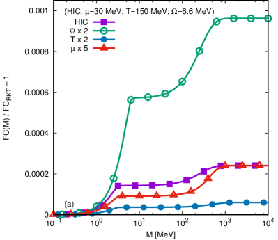
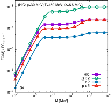
Figure 8: Relative difference of the quantum and kinetic theory fermion condensates, on the rotation axis, computed by numerically integrating Eqs. (180) and (55), respectively. The HIC parameters are indicated at the top of the images and the corresponding curve is represented using purple and filled squares. For each subsequent curve, only the parameter indicated in the legend is changed, compared to the original set. The results are represented in log-linear (a) and log-log (b) scale.

At vanishing mass, a comparison between Eqs. (184) and (57) indicates that the t.e.v. of the FC (divided by $M$) is identical with the RKT prediction for the trace of the SET (divided by $M^{2}$). At finite mass, it can be expected that this equality holds only approximately. Figure 8 presents the relative difference between the quantum and RKT predictions for the FC, evaluated on the rotation axis. It can be seen that there is a rapid increase from $0$ in the massless case to some plateau values. The first plateau occurs quite early, for $M\gtrsim 5\ {\rm MeV}$. The second plateau appears when $M\simeq T$. The values on these plateaus depend on the parameters of the system. Doubling $\Omega$ increases the plateaus by a factor of $4$, while doubling the temperature decreases the value, again by a factor of $4$, as can be seen from Fig. 8(a). Increasing the chemical potentials ($\mu_{V}=\mu_{H}$ is considered here) seems to lower the plateau in the central region, however, for $M\gtrsim 1\ {\rm GeV}$, it gives the same result as in the case of the HIC parameters. The increase from the massless limit to the first plateau seems to follow a power law of the form $\sim M^{3/2}$, as can be seen from Fig. 8(b).

9 Stress-energy tensor

The stress-energy tensor (SET) operator is defined as:

$$\widehat{T}_{{\hat{\alpha}}{\hat{\sigma}}}=\frac{i}{4}e_{{\hat{\alpha}}}^{\mu}e_{{\hat{\sigma}}}^{\nu}\left\{[\widehat{\overline{\Psi}},\gamma_{(\mu}\partial_{\nu)}\widehat{\Psi}]-[\partial_{(\mu}\widehat{\overline{\Psi}}\gamma_{\nu)},\widehat{\Psi}]\right\}.$$ (185)

The general expressions for the computation of the thermal expectation values (t.e.v.s) of the SET operator are presented in Subsec. 9.1. The analytical and numerical analyses of these expressions are presented in Subsections 9.2 and 9.3.

9.1 General analysis

The bilinear form defined in Eq. (87) which corresponds to the SET operator is

$$\mathcal{T}_{{\hat{\alpha}}{\hat{\sigma}}}(\psi,\chi)=\frac{i}{2}e_{\hat{\alpha}}^{\mu}e_{\hat{\sigma}}^{\nu}\left[\,\overline{\psi}\gamma_{(\mu}\partial_{\nu)}\chi-\partial_{(\mu}\overline{\psi}\gamma_{\nu)}\chi\right].$$ (186)

Substituting $\psi=\chi=V_{j}$ in the above equation and using the relations in Eq. (73), it can be shown that

$$\mathcal{T}_{{\hat{\alpha}}{\hat{\sigma}}}(V_{j},V_{j})=\mathcal{T}_{{\hat{\alpha}}{\hat{\sigma}}}(U_{\overline{\jmath}},U_{\overline{\jmath}})=-[\mathcal{T}_{{\hat{\alpha}}{\hat{\sigma}}}(U_{j},U_{j})]^{*}.$$ (187)

As in Sections 7 and 8, the second line of Eq. (101) does not contribute to the t.e.v. of the SET, which can be summarised as follows:

$$\braket{:\widehat{T}_{{\hat{\alpha}}{\hat{\sigma}}}:_{\Omega}}=\sum_{\lambda=\pm\frac{1}{2}}\sum_{m=-\infty}^{\infty}\int_{M}^{\infty}dE\,E\,{\rm sgn}(\widetilde{E})\left[\frac{1}{e^{\beta_{0}(|\widetilde{E}|-\mu_{\lambda;0})}+1}+\frac{1}{e^{\beta_{0}(|\widetilde{E}|+\mu_{\lambda;0})}+1}\right]\\ \times\int_{-p}^{p}dk\,\mathcal{T}_{{\hat{\alpha}}{\hat{\sigma}}}(U_{j},U_{j}).$$ (188)

Using the explicit expression for the modes $U_{j}$, given in Eq. (72), the following auxiliary expressions can be computed:

$$i\overline{U}_{j}\gamma_{{\hat{\alpha}}}e_{{\hat{t}}}^{\nu}\partial_{\nu}U_{j}= E_{j}\overline{U}_{j}\gamma_{{\hat{\alpha}}}U_{j},\qquad i\overline{U}_{j}\gamma_{{\hat{\alpha}}}e_{{\hat{z}}}^{\nu}\partial_{\nu}U_{j}=-k_{j}\overline{U}_{j}\gamma_{{\hat{\alpha}}}U_{j},$$

$$i\overline{U}_{j}\gamma_{{\hat{t}}}e_{{\hat{\rho}}}^{\nu}\partial_{\nu}U_{j}= -\frac{i\lambda_{j}k_{j}q_{j}}{4\pi^{2}p_{j}}J_{m_{j}}^{\times}(q_{j}\rho)$$

$$+\frac{i}{8\pi^{2}\rho}\left[\left(\frac{2\lambda_{j}k_{j}}{p_{j}}m_{j}-\frac{1}{2}\right)J_{m_{j}}^{+}(q_{j}\rho)+\left(m_{j}-\frac{\lambda_{j}k_{j}}{p_{j}}\right)J_{m_{j}}^{-}(q_{j}\rho)\right],$$

$$i\overline{U}_{j}\gamma_{{\hat{\rho}}}e_{{\hat{\rho}}}^{\nu}\partial_{\nu}U_{j}= \frac{q_{j}^{2}}{8\pi^{2}E_{j}}\left[J_{m_{j}}^{+}(q_{j}\rho)-\frac{m_{j}}{q_{j}\rho}J_{m_{j}}^{\times}(q_{j}\rho)\right],$$

$$i\overline{U}_{j}\gamma_{{\hat{\varphi}}}e_{{\hat{\rho}}}^{\nu}\partial_{\nu}U_{j}= -\frac{iq_{j}}{8\pi^{2}E_{j}\rho}\left[q_{j}\rho\,J_{m_{j}}^{-}(q_{j}\rho)-\frac{1}{2}J_{m_{j}}^{\times}(q_{j}\rho)\right],$$

$$i\overline{U}_{j}\gamma_{{\hat{z}}}e_{{\hat{\rho}}}^{\nu}\partial_{\nu}U_{j}= \frac{i\lambda_{j}q_{j}p_{j}}{4\pi^{2}E_{j}}J_{m_{j}}^{\times}(q_{j}\rho)$$

$$-\frac{i\lambda_{j}p_{j}}{4\pi^{2}E_{j}\rho}\left[\left(m_{j}-\frac{\lambda_{j}k_{j}}{p_{j}}\right)J_{m_{j}}^{+}(q_{j}\rho)+\left(\frac{2\lambda_{j}k_{j}}{p_{j}}m_{j}-\frac{1}{2}\right)J_{m_{j}}^{-}(q_{j}\rho)\right],$$

$$i\overline{U}_{j}\gamma_{{\hat{t}}}e_{{\hat{\varphi}}}^{\nu}\partial_{\nu}U_{j}= -\frac{1}{8\pi^{2}\rho}\left[\left(m_{j}-\frac{\lambda_{j}k_{j}}{p_{j}}\right)J_{m_{j}}^{+}(q_{j}\rho)+\left(\frac{2\lambda_{j}k_{j}}{p_{j}}m_{j}-\frac{1}{2}\right)J_{m_{j}}^{-}(q_{j}\rho)\right],$$

$$i\overline{U}_{j}\gamma_{{\hat{\rho}}}e_{{\hat{\varphi}}}^{\nu}\partial_{\nu}U_{j}= \frac{iq_{j}}{16\pi^{2}E_{j}\rho}J_{m_{j}}^{\times}(q_{j}\rho),$$

$$i\overline{U}_{j}\gamma_{{\hat{\varphi}}}e_{{\hat{\varphi}}}^{\nu}\partial_{\nu}U_{j}= \frac{m_{j}q_{j}}{8\pi^{2}E_{j}\rho}J_{m_{j}}^{\times}(q_{j}\rho),$$

$$i\overline{U}_{j}\gamma_{{\hat{z}}}e_{{\hat{\varphi}}}^{\nu}\partial_{\nu}U_{j}= \frac{\lambda_{j}p_{j}}{4\pi^{2}E_{j}\rho}\left[\left(\frac{2\lambda_{j}k_{j}}{p_{j}}m_{j}-\frac{1}{2}\right)J_{m_{j}}^{+}(q_{j}\rho)+\left(m_{j}-\frac{\lambda_{j}k_{j}}{p_{j}}\right)J_{m_{j}}^{-}(q_{j}\rho)\right].$$ (189)

The derivatives of the Bessel functions were replaced using the following identities:

$$J_{m-\frac{1}{2}}^{\prime}(q\rho)= -J_{m+\frac{1}{2}}(q\rho)+\frac{m-\frac{1}{2}}{q\rho}J_{m-\frac{1}{2}}(q\rho),$$

$$J_{m+\frac{1}{2}}^{\prime}(q\rho)= J_{m-\frac{1}{2}}(q\rho)-\frac{m+\frac{1}{2}}{q\rho}J_{m+\frac{1}{2}}(q\rho).$$ (190)

Since $\mathcal{T}_{{\hat{\alpha}}{\hat{\sigma}}}(U_{j},U_{j})={\rm Re}[i\overline{U}_{j}\gamma_{({\hat{\alpha}}}e_{{\hat{\sigma}})}^{\mu}\partial_{\mu}U_{j}]$, the terms proportional to the imaginary unit $i$ appearing in Eq. (189) can be ignored. The non-vanishing components of the bilinear form $\mathcal{T}_{{\hat{\alpha}}{\hat{\sigma}}}(U_{j},U_{j})$ are:

$$\mathcal{T}_{{\hat{t}}{\hat{t}}}(U_{j},U_{j})= \frac{E_{j}}{8\pi^{2}}\left[J_{m_{j}}^{+}(q_{j}\rho)+\frac{2\lambda_{j}k_{j}}{p_{j}}J_{m_{j}}^{-}(q_{j}\rho)\right],$$

$$\mathcal{T}_{{\hat{t}}{\hat{\varphi}}}(U_{j},U_{j})= -\frac{1}{16\pi^{2}\rho}\left[\left(m_{j}-\frac{\lambda_{j}k_{j}}{p_{j}}\right)J_{m_{j}}^{+}(q_{j}\rho)+\left(\frac{2\lambda_{j}k_{j}m_{j}}{p_{j}}-\frac{1}{2}\right)J_{m_{j}}^{-}(q_{j}\rho)\right]$$

$$-\frac{q_{j}}{16\pi^{2}}J_{m_{j}}^{\times}(q_{j}\rho),$$

$$\mathcal{T}_{{\hat{t}}{\hat{z}}}(U_{j},U_{j})= -\frac{\lambda_{j}(p^{2}_{j}+k_{j}^{2})}{8\pi^{2}p_{j}}J_{m_{j}}^{-}(q_{j}\rho)-\frac{k_{j}}{8\pi^{2}}J_{m_{j}}^{+}(q_{j}\rho),$$

$$\mathcal{T}_{{\hat{\rho}}{\hat{\rho}}}(U_{j},U_{j})= \frac{q_{j}^{2}}{8\pi^{2}E_{j}}\left[J_{m_{j}}^{+}(q_{j}\rho)-\frac{m_{j}}{q_{j}\rho}J_{m_{j}}^{\times}(q_{j}\rho)\right],$$

$$\mathcal{T}_{{\hat{\varphi}}{\hat{\varphi}}}(U_{j},U_{j})= \frac{q_{j}m_{j}}{8\pi^{2}\rho E_{j}}J_{m_{j}}^{\times}(q_{j}\rho),$$

$$\mathcal{T}_{{\hat{\varphi}}{\hat{z}}}(U_{j},U_{j})= \frac{\lambda_{j}p_{j}}{8\pi^{2}\rho E_{j}}\left[m_{j}J_{m_{j}}^{-}(q_{j}\rho)-\frac{1}{2}J_{m_{j}}^{+}(q_{j}\rho)\right]$$

$$+\frac{k_{j}}{16\pi^{2}\rho E_{j}}\left[q_{j}\rho J_{m_{j}}^{\times}(q_{j}\rho)-\frac{1}{2}J_{m_{j}}^{-}(q_{j}\rho)+m_{j}J_{m_{j}}^{+}(q_{j}\rho)\right],$$

$$\mathcal{T}_{{\hat{z}}{\hat{z}}}(U_{j},U_{j})= \frac{k_{j}^{2}}{8\pi^{2}E_{j}}J_{m_{j}}^{+}(q_{j}\rho)+\frac{\lambda_{j}k_{j}p_{j}}{4\pi^{2}E_{j}}J_{m_{j}}^{-}(q_{j}\rho).$$ (191)

The terms appearing in Eq. (191) which are odd with respect to $k_{j}\rightarrow-k_{j}$ do not contribute to the t.e.v. of the SET. Starting from the above expressions, it is possible to show that the t.e.v.s $\braket{:\widehat{T}_{{\hat{\rho}}{\hat{\rho}}}:}$ and $\braket{:\widehat{T}_{{\hat{z}}{\hat{z}}}:}$ are exactly equal. This can be seen by first noting that

$$J_{m}^{-}(z)=\frac{1}{2m}\frac{d}{dz}[zJ_{m}^{+}(z)]=\frac{1}{2z}\frac{d}{dz}[zJ_{m}^{\times}(z)].$$ (192)

The above relations can be derived using the properties of the derivatives of the Bessel functions $J_{m-1/2}(z)$ and $J_{m+1/2}(z)$ given in Eq. (190). Next, $I_{m}(p)$ is introduced as follows:

$$I_{m}(p)=\frac{1}{2}\int_{-p}^{p}dk\,k^{2}J_{m}^{-}(q\rho)=\int_{0}^{p}dk\,k^{2}J_{m}^{-}(q\rho),$$ (193)

where the last equality follows after noting that the integrand is even with respect to $k$. Replacing now $J_{m}^{-}(q\rho)$ using the two expressions in Eq. (192) and using integration by parts to remove the derivative term, it can be shown that

$$I_{m}(p)=\frac{1}{2m}\int_{0}^{p}dk(q^{2}-k^{2})J_{m}^{+}(q\rho)=\frac{1}{2\rho}\int_{0}^{p}dk\,q\,J_{m}^{\times}(q\rho).$$ (194)

Rearranging the above expressions, it can be seen that

$$\int_{-p}^{p}dk\,\mathcal{T}_{{\hat{\rho}}{\hat{\rho}}}(U_{j},U_{j})=\int_{-p}^{p}dk\,\mathcal{T}_{{\hat{z}}{\hat{z}}}(U_{j},U_{j}).$$ (195)

Thus, it is easy to conclude that

$$\braket{:\widehat{T}_{{\hat{\rho}}{\hat{\rho}}}:_{\Omega}}=\braket{:\widehat{T}_{{\hat{z}}{\hat{z}}}:_{\Omega}},$$ (196)

the above relation being valid for all values of $\rho$, $\Omega$, $M$, $\beta_{0}$, $\mu_{V,0}$ and $\mu_{H,0}$.

For a given velocity field $u^{\hat{\alpha}}$, the SET can be decomposed as follows:

$$\braket{:\widehat{T}^{{\hat{\alpha}}{\hat{\sigma}}}:_{\Omega}}=E\,u^{\hat{\alpha}}u^{\hat{\sigma}}-(P+\overline{\omega})\Delta^{{\hat{\alpha}}{\hat{\sigma}}}+\Pi^{{\hat{\alpha}}{\hat{\sigma}}}+u^{\hat{\alpha}}W^{\hat{\sigma}}+u^{\hat{\sigma}}W^{\hat{\alpha}},$$ (197)

where $E$ and $P$ are the usual energy density and pressure, $W^{\hat{\alpha}}$ represents the heat flux in the local rest frame, $\overline{\omega}$ is the dynamic pressure and $\Pi^{{\hat{\alpha}}{\hat{\sigma}}}$ is the pressure deviator, which is traceless by construction. The tensor $\Delta^{{\hat{\alpha}}{\hat{\sigma}}}=\eta^{{\hat{\alpha}}{\hat{\sigma}}}-u^{\hat{\alpha}}u^{\hat{\sigma}}$ is a projector on the hypersurface orthogonal to $u^{\hat{\alpha}}$. The anomalous contributions $\Pi^{{\hat{\alpha}}{\hat{\sigma}}}$ and $W^{\hat{\alpha}}$ are also orthogonal to $u^{\hat{\alpha}}$, by construction. The isotropic pressure $P+\overline{\omega}$ is given as the sum of the hydrostatic pressure $P$, which is computed using the equation of state of the fluid, and of the dynamic pressure $\overline{\omega}$, which in general depenends on the divergence of the velocity. With this convention, the pressure deviator is considered to be traceless. It should be noted that for ultrarelativistic fluids, the SET is traceless (this is true in the quantum case as well since the Dirac field is conformally coupled) and $E=3P$. Since $T^{{\hat{\alpha}}}{}_{\hat{\alpha}}=E-3(P+\overline{\omega})$, it can be seen that $\overline{\omega}=0$ for ultrarelativistic (massless) fluid constituents. Furthermore, for massive fluid constituents, $\overline{\omega}$ is usually related to the expansion of the fluid rezzolla13 , which vanishes in the case of rigid rotation. Thus, for the rest of this section, the relation $\overline{\omega}=0$ is assumed to hold true.

The macroscopic quantities can be extracted from $T^{{\hat{\alpha}}{\hat{\sigma}}}$ as follows:

$$E= \braket{:\widehat{T}_{{\hat{\alpha}}{\hat{\sigma}}}:_{\Omega}}u^{\hat{\alpha}}u^{\hat{\sigma}}, P+\overline{\omega}= -\frac{1}{3}\Delta^{{\hat{\alpha}}{\hat{\sigma}}}\braket{:\widehat{T}_{{\hat{\alpha}}{\hat{\sigma}}}:_{\Omega}},$$

$$W^{\hat{\alpha}}= \Delta^{{\hat{\alpha}}{\hat{\sigma}}}u^{\hat{\lambda}}\braket{:\widehat{T}_{{\hat{\sigma}}{\hat{\lambda}}}:_{\Omega}}, \Pi_{{\hat{\alpha}}{\hat{\sigma}}}= \braket{:\widehat{T}_{\braket{{\hat{\alpha}}{\hat{\sigma}}}}:_{\Omega}},$$ (198)

where the notation $A_{\braket{{\hat{\alpha}}{\hat{\sigma}}}}$ for a general two-tensor refers to:

$$A_{\braket{{\hat{\alpha}}{\hat{\sigma}}}}=\frac{1}{2}\left[\left(\Delta_{{\hat{\alpha}}{\hat{\beta}}}\Delta_{{\hat{\sigma}}{\hat{\gamma}}}+\Delta_{{\hat{\sigma}}{\hat{\beta}}}\Delta_{{\hat{\alpha}}{\hat{\gamma}}}\right)-\frac{2}{3}\Delta_{{\hat{\alpha}}{\hat{\sigma}}}\Delta_{{\hat{\beta}}{\hat{\gamma}}}\right]A^{{\hat{\beta}}{\hat{\gamma}}}.$$ (199)

The anomalous terms $W^{\hat{\alpha}}$ and $\Pi^{{\hat{\alpha}}{\hat{\sigma}}}$ can be further decomposed with respect to the tetrad formed by $u$, $a$, $\omega$ and $\tau$, introduced in Sec. 2. Noting that $W\cdot u=0$ and that $\braket{:\widehat{T}_{{\hat{\rho}}{\hat{\alpha}}}:_{\Omega}}=0$ when $\alpha\neq\rho$, the most general decomposition for $W$ is

$$W^{\hat{\alpha}}= \sigma_{\varepsilon}^{\tau}\tau^{\hat{\alpha}}+\sigma_{\varepsilon}^{\omega}\omega^{\hat{\alpha}},$$

$$\sigma_{\varepsilon}^{\tau}= \frac{1}{\Omega^{2}\Gamma^{2}}\left[\braket{:\widehat{T}_{{\hat{t}}{\hat{t}}}:_{\Omega}}+\braket{:\widehat{T}_{{\hat{\varphi}}{\hat{\varphi}}}:_{\Omega}}+\frac{1+\rho^{2}\Omega^{2}}{\rho\Omega}\braket{:\widehat{T}_{{\hat{t}}{\hat{\varphi}}}:_{\Omega}}\right],$$

$$\sigma_{\varepsilon}^{\omega}= -\frac{1}{\Omega\Gamma}\left[\braket{:\widehat{T}_{{\hat{t}}{\hat{z}}}:_{\Omega}}+\rho\Omega\braket{:\widehat{T}_{{\hat{\varphi}}{\hat{z}}}:_{\Omega}}\right],$$ (200)

where $\sigma_{\varepsilon}^{\tau}$ and $\sigma_{\varepsilon}^{\omega}$ are the circular and vortical heat conductivities. In the case of $\Pi^{{\hat{\alpha}}{\hat{\sigma}}}$, the orthogonality to $u^{\hat{\alpha}}$ and the tracelessness condition, together with the consideration that $\braket{:\widehat{T}_{{\hat{\alpha}}{\hat{\rho}}}:_{\Omega}}=0$ for all $\alpha\neq\rho$, allow $\Pi^{{\hat{\alpha}}{\hat{\sigma}}}$ to be written as:

$$\Pi^{{\hat{\alpha}}{\hat{\sigma}}}=Aa^{\hat{\alpha}}a^{\hat{\sigma}}+B\tau^{\hat{\alpha}}\tau^{\hat{\sigma}}+C\omega^{\hat{\alpha}}\omega^{\hat{\sigma}}+D(\tau^{\hat{\alpha}}\omega^{\hat{\sigma}}+\tau^{\hat{\sigma}}\omega^{\hat{\alpha}}).$$ (201)

Noting that $\braket{:\widehat{T}_{{\hat{\rho}}{\hat{\rho}}}:_{\Omega}}=P+\Pi_{{\hat{\rho}}{\hat{\rho}}}$ and $\braket{:\widehat{T}_{{\hat{z}}{\hat{z}}}:_{\Omega}}=P+\Pi_{{\hat{z}}{\hat{z}}}$ are equal by virtue of Eq. (196), it can be seen that $\Pi_{{\hat{\rho}}{\hat{\rho}}}=\Pi_{{\hat{z}}{\hat{z}}}$, such that

$$C=\rho^{2}\Omega^{2}A.$$ (202)

The tracelessness condition gives

$$A=-\frac{1}{2}B\Omega^{2}\Gamma^{4}=\frac{\omega^{2}}{2}B\Rightarrow C=\frac{a^{2}}{2}B.$$ (203)

Thus, only two degrees of freedom are required to describe $\Pi^{{\hat{\alpha}}{\hat{\sigma}}}$, which are introduced below:

$$\Pi^{{\hat{\alpha}}{\hat{\sigma}}}=\Pi_{1}\left(\tau^{\hat{\alpha}}\tau^{\hat{\sigma}}+\frac{\omega^{2}}{2}a^{\hat{\alpha}}a^{\hat{\sigma}}+\frac{a^{2}}{2}\omega^{\hat{\alpha}}\omega^{\hat{\sigma}}\right)+\Pi_{2}(\tau^{\hat{\alpha}}\omega^{\hat{\sigma}}+\tau^{\hat{\sigma}}\omega^{\hat{\alpha}}),$$ (204)

where $\Pi_{1}$ and $\Pi_{2}$ can be obtained from the components of the SET, e.g., through:

$$\Pi_{1}=\frac{2(P-\braket{:\widehat{T}_{{\hat{z}}{\hat{z}}}:_{\Omega}})}{\Omega^{4}\Gamma^{6}(\Gamma^{2}-1)},\qquad\Pi_{2}=-\frac{\braket{:\widehat{T}_{{\hat{\varphi}}{\hat{z}}}:_{\Omega}}+\rho\Omega\braket{:\widehat{T}_{{\hat{t}}{\hat{z}}}:_{\Omega}}}{\rho\Omega^{4}\Gamma^{5}}.$$ (205)

9.2 Small mass limit

Following the procedure which is by now familiar, the t.e.v.s of the components of the SET are computed in the small mass regime. Starting from their expressions with respect to the rotating vacuum, given in Eq. (188), the transition to the Minkowski vacuum can be performed. After expanding the Fermi-Dirac factors via Eq. (104), the summation over $m$ and integration over $k$ can be performed using Eqs. (108) and (112):

$$\begin{pmatrix}\braket{:\widehat{T}_{{\hat{t}}{\hat{t}}}:_{M}}&\braket{:\widehat{T}_{{\hat{\rho}}{\hat{\rho}}}:_{M}}\\ \braket{:\widehat{T}_{{\hat{\varphi}}{\hat{\varphi}}}:_{M}}&-\braket{:\widehat{T}_{{\hat{t}}{\hat{\varphi}}}:_{M}}/\rho\Omega\end{pmatrix}=\frac{1}{2\pi^{2}}\sum_{\lambda=\pm\frac{1}{2}}\sum_{j=0}^{\infty}(\rho\Omega)^{2j}\sum_{n=0}^{\infty}\frac{\Omega^{2n}s_{n+j,j}^{+}}{(2n+2j+1)!}\\ \times\int_{M}^{\infty}dE\,p^{2j+1}\frac{d^{2n+2j}}{dE^{2n+2j}}\left[\frac{1}{e^{\beta_{0}(E-\mu_{\lambda,0})}+1}+\frac{1}{e^{\beta_{0}(E+\mu_{\lambda,0})}+1}\right]\\ \times\begin{pmatrix}\displaystyle\frac{2n+2j+1}{2j+1}E^{2}&\displaystyle\frac{2n+2j+1}{(2j+1)(2j+3)}p^{2}\vskip 3.0pt plus 1.0pt minus 1.0pt\\ \displaystyle\frac{2n+2j+1}{2j+3}p^{2}&\displaystyle\frac{p^{2}}{2j+3}+E^{2}+\frac{j}{4(\rho p)^{2}}\left[p^{2}+E^{2}(2j+1)\right]\end{pmatrix},$$ (206)

while $\braket{:\widehat{T}_{{\hat{z}}{\hat{z}}}:_{M}}=\braket{:\widehat{T}_{{\hat{\rho}}{\hat{\rho}}}:_{M}}$, as shown in Eq. (196). The $M$ subscript indicates that the above expressions are computed with respect to the Minkowski vacuum, as discussed in Sec. 5.3. In obtaining the expression for $\braket{:\widehat{T}_{{\hat{t}}{\hat{\varphi}}}:_{M}}$, integration by parts, Eq. (111) and the relation $s_{n,0}^{+}=2^{-2n}$ were used. After changing the integration variable to $p$, Eq. (106) can be used to analyse the small mass regime. After employing integration by parts $2j$ times in the integral with respect to $p$, it is not difficult to see that the summation over $n$ terminates at a finite value of $n$. This is because

$$\int_{0}^{\infty}dp\,p^{3}\frac{d^{2n}}{dp^{2n}}\left[\frac{1}{e^{\beta_{0}(p-\mu_{\lambda,0})}+1}+\frac{1}{e^{\beta_{0}(p+\mu_{\lambda,0})}+1}\right]=\begin{cases}\displaystyle\frac{2}{\beta_{0}^{4}}I_{1}^{+}(\beta_{0}\mu_{\lambda,0}),&n=0,\vskip 3.0pt plus 1.0pt minus 1.0pt\\ \displaystyle\frac{12}{\beta_{0}^{2}}I_{0}^{+}(\beta_{0}\mu_{\lambda,0}),&n=1,\vskip 3.0pt plus 1.0pt minus 1.0pt\\ 6,&n=2,\\ 0,&n>2.\end{cases}$$ (207)

The last equality follows from noting that $(1+e^{-a})^{-1}+(1+e^{a})^{-1}=1$. Taking into account that the $n=2$ term makes a purely vacuum contribution, the following exact results are obtained for the t.e.v.s with respect to the rotating vacuum:

$$\braket{:\widehat{T}_{{\hat{t}}{\hat{t}}}:_{\Omega}}= \Gamma^{2}E_{\rm RKT}+P_{\rm RKT}(\Gamma^{2}-1)+\frac{\Omega^{2}\Gamma^{2}}{8}\left[T^{2}+\frac{3(\mu_{V}^{2}+\mu_{H}^{2})}{\pi^{2}}\right]\left(\frac{8}{3}\Gamma^{4}-\frac{16}{9}\Gamma^{2}+\frac{1}{9}\right)$$

$$\braket{:\widehat{T}_{{\hat{t}}{\hat{\varphi}}}:_{\Omega}}= -\rho\Omega\Gamma^{2}\Bigg{\{}E_{\rm RKT}+P_{\rm RKT}+\frac{2\Omega^{2}\Gamma^{2}}{9}\left[T^{2}+\frac{3(\mu_{V}^{2}+\mu_{H}^{2})}{\pi^{2}}\right]\left(\frac{3}{2}\Gamma^{2}-\frac{1}{2}\right)\Bigg{\}},$$

$$\braket{:\widehat{T}_{{\hat{\rho}}{\hat{\rho}}}:_{\Omega}}= P_{\rm RKT}+\frac{\Omega^{2}\Gamma^{2}}{24}\left[T^{2}+\frac{3(\mu_{V}^{2}+\mu_{H}^{2})}{\pi^{2}}\right]\left(\frac{4}{3}\Gamma^{2}-\frac{1}{3}\right),$$

$$\braket{:\widehat{T}_{{\hat{\varphi}}{\hat{\varphi}}}:_{\Omega}}= \Gamma^{2}P_{\rm RKT}+E_{\rm RKT}(\Gamma^{2}-1)+\frac{\Omega^{2}\Gamma^{2}}{24}\left[T^{2}+\frac{3(\mu_{V}^{2}+\mu_{H}^{2})}{\pi^{2}}\right]\left(8\Gamma^{4}-8\Gamma^{2}+1\right),$$ (208)

while $\braket{:\widehat{T}_{{\hat{z}}{\hat{z}}}:_{\Omega}}=\braket{:\widehat{T}_{{\hat{\rho}}{\hat{\rho}}}:_{\Omega}}$. The $O(M^{2})$ corrections computed from Eq. (206) using the technique described in Eq. (106) are absorbed in the RKT predictions $E_{\rm RKT}$ and $P_{\rm RKT}$ for the energy density and pressure, given in Eq. (70). The following expressions can be obtained:

$$E= E_{\rm RKT}+\Delta E, P= P_{\rm RKT}+\Delta P,$$

$$\Delta E= \frac{\bm{a}^{2}+3\bm{\omega}^{2}}{24}\left[T^{2}+\frac{3(\mu_{V}^{2}+\mu_{H}^{2})}{\pi^{2}}\right]+O(M^{4}), \Delta P= \frac{1}{3}\Delta E+O(M^{4}),$$

$$\sigma_{\varepsilon}^{\tau}= -\frac{1}{18}\left[T^{2}+\frac{3(\mu_{V}^{2}+\mu_{H}^{2})}{\pi^{2}}\right]+O(M^{4}), \Pi_{1}= O(M^{4}).$$ (209)

Comparing Eq. (209) and Eq. (160), it is interesting to note that $\sigma_{\varepsilon}^{\tau}=-\frac{1}{3}\sigma^{\omega}_{A}$.

There is a set of components which is non-vanishing only when $\mu_{H,0}\neq 0$. These can be computed using:

$$\begin{pmatrix}\braket{:\widehat{T}_{{\hat{t}}{\hat{z}}}:_{\Omega}}\\ \braket{:\widehat{T}_{{\hat{\varphi}}{\hat{z}}}:_{\Omega}}\end{pmatrix}=\frac{1}{8\pi^{2}\rho}\sum_{\lambda=\pm\frac{1}{2}}2\lambda\sum_{j=0}^{\infty}(\rho\Omega)^{2j}\sum_{n=0}^{\infty}\frac{\Omega^{2n}s_{n+j,j}^{+}}{(2n+2j+1)!}\int_{M}^{\infty}dE\,p^{2j}\\ \times\frac{d^{2n+2j}}{dE^{2n+2j}}\left[\frac{1}{e^{\beta_{0}(E-\mu_{\lambda,0})}+1}+\frac{1}{e^{\beta_{0}(E+\mu_{\lambda,0})}+1}\right]\\ \times\begin{pmatrix}\displaystyle-\rho\Omega\frac{2j+4}{2j+3}[2(j+1)E^{2}+p^{2}]\vskip 3.0pt plus 1.0pt minus 1.0pt\\ \displaystyle 2j\frac{2n+2j+1}{2j+1}p^{2}\end{pmatrix}.$$ (210)

As in the previous subsections, the sum over $n$ does not terminate at finite $n$. Instead, the first two terms in this sum give:

$$\braket{:\widehat{T}_{{\hat{t}}{\hat{z}}}:_{\Omega}}= -\frac{\Omega\Gamma^{3}}{\pi^{2}}\sum_{\lambda}2\lambda\left\{T^{3}I_{1/2}^{+}(\beta\mu_{\lambda})+\frac{\Omega^{2}T}{12}\Gamma^{2}(6\Gamma^{2}-5)I_{-1/2}^{+}(\beta\mu_{\lambda})\right.$$

$$\left.-\frac{M^{2}T}{8(\Gamma^{2}-1)}\left[2\Gamma^{2}-1-\frac{{\rm arcsinh}(\rho\Omega\Gamma)}{\rho\Omega\Gamma^{2}}\right]I_{-1/2}^{+}(\beta\mu_{\lambda})+O(\Omega^{4},M^{4},\Omega^{2}M^{2})\right\},$$

$$\braket{:\widehat{T}_{{\hat{\varphi}}{\hat{z}}}:_{\Omega}}= \frac{\rho\Omega^{2}\Gamma^{3}}{\pi^{2}}\sum_{\lambda}2\lambda\left\{T^{3}I_{1/2}^{+}(\beta\mu_{\lambda})+\frac{\Omega^{2}T}{12}\Gamma^{2}(6\Gamma^{2}-1)I_{-1/2}^{+}(\beta\mu_{\lambda})\right.$$

$$\left.-\frac{M^{2}T}{8(\Gamma^{2}-1)}\left[2\Gamma^{2}-1-\frac{{\rm arcsinh}(\rho\Omega\Gamma)}{\rho\Omega\Gamma^{2}}\right]I_{-1/2}^{+}(\beta\mu_{\lambda})+O(\Omega^{4},M^{4},\Omega^{2}M^{2})\right\}.$$ (211)

From the above, the coefficients $\sigma_{\varepsilon}^{\omega}$ and $\Pi_{2}$ can be obtained:

$$\sigma_{\varepsilon}^{\omega}= \frac{T^{3}}{\pi^{2}}\sum_{\lambda=\pm\frac{1}{2}}2\lambda I_{1/2}^{+}(\beta\mu_{\lambda})+\frac{T}{12\pi^{2}}(\bm{\omega}^{2}+\bm{a}^{2})\sum_{\lambda=\pm\frac{1}{2}}2\lambda I_{-1/2}^{+}(\beta\mu_{\lambda})$$

$$-\frac{M^{2}T}{8\pi^{2}(\Gamma^{2}-1)}\left[2\Gamma^{2}-1-\frac{{\rm arcsinh}(\rho\Omega\Gamma)}{\rho\Omega\Gamma^{2}}\right]\sum_{\lambda=\pm\frac{1}{2}}2\lambda I_{-1/2}^{+}(\beta\mu_{\lambda})+O(\Omega^{4},M^{4},\Omega^{2}M^{2}),$$

$$\Pi_{2}= -\frac{T}{3\pi^{2}}\sum_{\lambda=\pm\frac{1}{2}}2\lambda I_{-1/2}^{+}(\beta\mu_{\lambda})+O(\Omega^{2},M^{2}).$$ (212)

The exact expressions for $I_{\pm 1/2}^{+}$ given in Eq. (246) can be used to obtain:

$$\sigma_{\varepsilon}^{\omega}= -\frac{T^{3}}{\pi^{2}}\left[{\rm Li}_{3}(-e^{-\beta\mu_{+}})-{\rm Li}_{3}(-e^{-\beta\mu_{-}})+{\rm Li}_{3}(-e^{\beta\mu_{+}})-{\rm Li}_{3}(-e^{\beta\mu_{-}})\right]$$

$$+\frac{T}{12\pi^{2}}\left\{\bm{\omega}^{2}+\bm{a}^{2}-\frac{3M^{2}}{2(\Gamma^{2}-1)}\left[2\Gamma^{2}-1-\frac{{\rm arcsinh}(\rho\Omega\Gamma)}{\rho\Omega\Gamma^{2}}\right]\right\}\ln\left[\frac{\cosh\frac{\beta}{2}(\mu_{V}+\mu_{H})}{\cosh\frac{\beta}{2}(\mu_{V}-\mu_{H})}\right]$$

$$+O(\Omega^{4},M^{4},\Omega^{2}M^{2}),$$

$$\Pi_{2}= -\frac{T}{3\pi^{2}}\ln\left[\frac{\cosh\frac{\beta}{2}(\mu_{V}+\mu_{H})}{\cosh\frac{\beta}{2}(\mu_{V}-\mu_{H})}\right]+O(\Omega^{2},M^{2}).$$ (213)

The large temperature limit of the above expressions is:

$$\sigma_{\varepsilon}^{\omega}= \frac{4\mu_{V}\mu_{H}T}{\pi^{2}}\ln 2+\frac{\mu_{V}\mu_{H}}{6\pi^{2}T}\left(\mu_{V}^{2}+\mu_{H}^{2}+\frac{\bm{\omega}^{2}+\bm{a}^{2}}{4}\right)$$

$$-\frac{\mu_{V}\mu_{H}M^{2}}{16\pi^{2}T(\Gamma^{2}-1)}\left[2\Gamma^{2}-1-\frac{{\rm arcsinh}(\rho\Omega\Gamma)}{\rho\Omega\Gamma^{2}}\right]+O(T^{-3}),$$

$$\Pi_{2}= -\frac{\mu_{V}\mu_{H}}{6\pi^{2}T}+O(T^{-3}).$$ (214)

It is interesting to note that $\sigma_{\varepsilon}^{\omega}$ differs from $Q_{A}$, given in Eq. (167), only through the mass correction and the terms proportional to $\bm{\omega}^{2}$ and $\bm{a}^{2}$.

The results derived in Eq. (213) are valid only at small $\Omega$. Expressions for $\sigma_{\varepsilon}^{\omega}$ and $\Pi_{2}$ which are exact on the rotation axis can be derived by noting that

$$\sigma_{\varepsilon}^{\omega}\rfloor_{\rho=0}=-\frac{1}{\Omega\Gamma}\left.\braket{:\widehat{T}_{{\hat{t}}{\hat{z}}}:_{\Omega}}\right\rfloor_{\rho=0},\qquad\Pi_{2}\rfloor_{\rho=0}=-\left(\frac{\braket{:\widehat{T}_{{\hat{\varphi}}{\hat{z}}}:_{\Omega}}}{\rho\Omega^{4}\Gamma^{5}}+\frac{\braket{:\widehat{T}_{{\hat{t}}{\hat{z}}}:_{\Omega}}}{\Omega^{3}\Gamma^{5}}\right)_{\rho=0}.$$ (215)

Starting from Eq. (188):

$$\begin{pmatrix}\braket{:\widehat{T}_{{\hat{t}}{\hat{z}}}:_{\Omega}}\\ \braket{:\widehat{T}_{{\hat{\varphi}}{\hat{z}}}:_{\Omega}}/\rho\Omega\end{pmatrix}=\frac{1}{8\pi^{2}}\sum_{\lambda=\pm\frac{1}{2}}2\lambda\sum_{m=-\infty}^{\infty}\int_{M}^{\infty}dE\,p\,\left[\frac{1}{e^{\beta_{0}(\widetilde{E}-\mu_{\lambda;0})}+1}+\frac{1}{e^{\beta_{0}(\widetilde{E}+\mu_{\lambda;0})}+1}\right]\\ \times\int_{0}^{p}dk\begin{pmatrix}-E\left(1+\frac{k^{2}}{p^{2}}\right)J_{m}^{-}(q\rho)\\ \frac{1}{\rho^{2}\Omega}\left[mJ_{m}^{-}(q\rho)-\frac{1}{2}J_{m}^{+}(q\rho)\right]\end{pmatrix}$$ (216)

and noting that $J_{\pm 1/2}^{-}(z)=\pm 1$ and

$$\left[mJ_{m}^{-}(q\rho)-\frac{1}{2}J_{m}^{+}(q\rho)\right]_{m=\pm\frac{1}{2}}=-\left[mJ_{m}^{-}(q\rho)-\frac{1}{2}J_{m}^{+}(q\rho)\right]_{m=\pm\frac{3}{2}}=-\left(\frac{q\rho}{2}\right)^{2}+\dots,$$ (217)

the following expressions can be obtained:

$$\braket{:\widehat{T}_{{\hat{t}}{\hat{z}}}:_{\Omega}}_{\rho=0}= -\frac{1}{3\pi^{2}}\sum_{\lambda=\pm\frac{1}{2}}2\lambda\int_{M}^{\infty}dE\,Ep^{2}\left[f^{-}_{\beta_{0}}\left(\mu_{\lambda;0}+\frac{\Omega}{2}\right)-f^{-}_{\beta_{0}}\left(\mu_{\lambda;0}-\frac{\Omega}{2}\right)\right],$$

$$\left.\frac{\braket{:\widehat{T}_{{\hat{\varphi}}{\hat{z}}}:_{\Omega}}}{\rho\Omega}\right\rfloor_{\rho=0}= -\frac{1}{24\pi^{2}\Omega}\sum_{\lambda=\pm\frac{1}{2}}2\lambda\sum_{\sigma_{\Omega}=\pm 1}\int_{M}^{\infty}dE\,p^{4}$$

$$\times\left[f^{+}_{\beta_{0}}\left(\mu_{\lambda;0}+\sigma_{\Omega}\frac{\Omega}{2}\right)-f^{+}_{\beta_{0}}\left(\mu_{\lambda;0}+\sigma_{\Omega}\frac{3\Omega}{2}\right)\right],$$ (218)

where the notation $f^{\pm}_{\beta_{0}}(a)$ was introduced in Eq. (135). Using Eq. (63) to expand $f^{\pm}_{\beta_{0}}(a)$ and Eq. (64) to perform the sum over helicities, the following result can be obtained:

$$\braket{:\widehat{T}_{{\hat{t}}{\hat{z}}}:_{\Omega}}_{\rho=0}= \frac{1}{\pi^{2}\beta_{0}^{4}}\sum_{\sigma_{\Omega}=\pm 1}\sigma_{\Omega}\sum_{\sigma_{V}=\pm 1}\sigma_{V}\sum_{\sigma_{H}=\pm 1}\sigma_{H}\Bigg{[}{\rm Li}_{4}(-e^{\zeta_{1/2}})$$

$$+\beta_{0}M{\rm Li}_{3}(-e^{\zeta_{1/2}})+\frac{(\beta_{0}M)^{2}}{3}{\rm Li}_{2}(-e^{\zeta_{1/2}})\Bigg{]},$$

$$\left.\frac{\braket{:\widehat{T}_{{\hat{\varphi}}{\hat{z}}}:_{\Omega}}}{\rho\Omega}\right\rfloor_{\rho=0}= -\frac{1}{2\pi^{2}\Omega\beta_{0}^{5}}\sum_{\sigma_{\Omega}=\pm 1}\sum_{\sigma_{V}=\pm 1}\sigma_{V}\sum_{\sigma_{H}=\pm 1}\sigma_{H}\Bigg{\{}{\rm Li}_{5}(-e^{\zeta_{3/2}})-{\rm Li}_{5}(-e^{\zeta_{1/2}})$$

$$+\beta_{0}M[{\rm Li}_{4}(-e^{\zeta_{3/2}})-{\rm Li}_{4}(-e^{\zeta_{1/2}})]+\frac{(\beta_{0}M)^{2}}{3}[{\rm Li}_{3}(-e^{\zeta_{3/2}})-{\rm Li}_{3}(-e^{\zeta_{1/2}})]\Bigg{\}},$$ (219)

where $\zeta_{m}=\beta_{0}(\sigma_{V}\mu_{V}+\sigma_{H}\mu_{H}+m\sigma_{\Omega}\Omega-M)$. At large temperatures, the following limits can be obtained:

$$\sigma_{\varepsilon}^{\omega}\rfloor_{\rho=0}= \frac{4\mu_{V}\mu_{H}T}{\pi^{2}}\ln 2+\frac{\mu_{V}\mu_{H}}{6\pi^{2}T}\left(\mu_{V}^{2}+\mu_{H}^{2}+\frac{\Omega^{2}}{4}-M^{2}\right)+O(T^{-3}),$$

$$\Pi_{2}\rfloor_{\rho=0}= -\frac{\mu_{V}\mu_{H}}{6\pi^{2}T}+\frac{\mu_{V}\mu_{H}}{72\pi^{2}T^{3}}\left(\mu_{V}^{2}+\mu_{H}^{2}+\frac{11\Omega^{2}}{20}-M^{2}\right)+O(T^{-4}),$$ (220)

in agreement with Eq. (214).

In summary, the SET for the Dirac field can be written as:

$$\braket{:\widehat{T}_{{\hat{\alpha}}{\hat{\sigma}}}:_{\Omega}}= \left(E_{\rm RKT}+\Delta E\right)u_{\hat{\alpha}}u_{\hat{\sigma}}-(P_{\rm RKT}+\Delta P)\Delta_{{\hat{\alpha}}{\hat{\sigma}}}+\Pi_{{\hat{\alpha}}{\hat{\sigma}}}+u_{{\hat{\alpha}}}W_{{\hat{\sigma}}}+u_{\hat{\sigma}}W_{\hat{\alpha}},$$

$$E_{\rm RKT}= \left[\frac{7\pi^{2}T^{4}}{60}+\frac{T^{2}}{2}(\mu_{V}^{2}+\mu_{H}^{2})+\frac{\mu_{V}^{4}+6\mu_{V}^{2}\mu_{H}^{2}+\mu_{H}^{4}}{4\pi^{2}}\right]-\frac{M^{2}}{12}\left[T^{2}+\frac{3(\mu_{V}^{2}+\mu_{H}^{2})}{\pi^{2}}\right],$$

$$\Delta E= \frac{\bm{a}^{2}+3\bm{\omega}^{2}}{24}\left[T^{2}+\frac{3(\mu_{V}^{2}+\mu_{H}^{2})}{\pi^{2}}\right],\qquad\Delta P=\frac{1}{3}\Delta E,$$

$$\Pi_{{\hat{\alpha}}{\hat{\sigma}}}= -\frac{\mu_{V}\mu_{H}}{6\pi^{2}T}(\tau_{{\hat{\alpha}}}\omega_{{\hat{\sigma}}}+\omega_{\hat{\alpha}}\tau_{\hat{\sigma}}),$$

$$W_{\hat{\alpha}}= -\frac{1}{18}\left[T^{2}+\frac{3(\mu_{V}^{2}+\mu_{H}^{2})}{\pi^{2}}\right]\tau_{\hat{\alpha}}+\frac{4\mu_{V}\mu_{H}T}{\pi^{2}}(\ln 2)\omega_{\hat{\alpha}}.$$ (221)

Only the leading order terms with respect to $T$ of $\Pi_{{\hat{\alpha}}{\hat{\sigma}}}$ and $\sigma_{\varepsilon}^{\omega}$ were included above. The corrections due to the mass are of order $O(M^{4})$. It is worth noting that, in the limit when $\mu_{H}=M=0$, the results in Eq. (221) reproduce the vanishing axial potential limit of Eq. (4.5) and Tables 2 and 3 from Ref. buzzegoli18 .

9.3 Numerical analysis

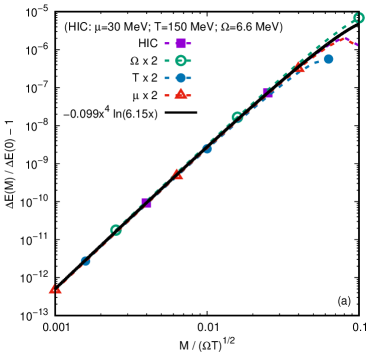
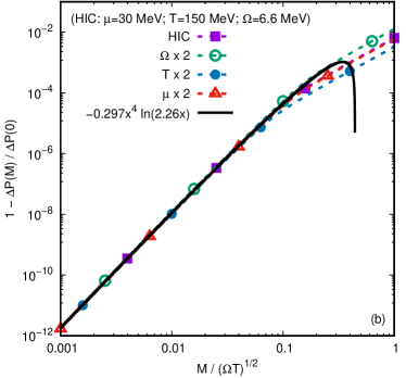
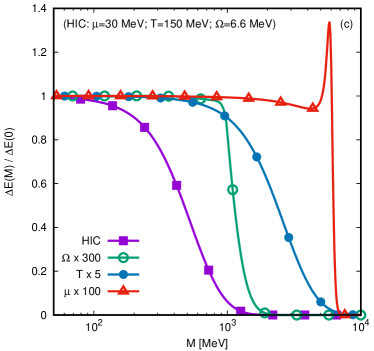
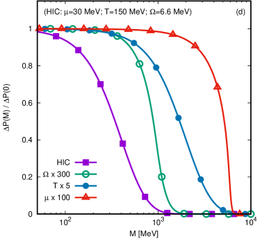
Figure 9: (Top line) Relative mass corrections (a) $\Delta E(M)/\Delta E(0)-1$ and (b) $1-\Delta P(M)/\Delta P(0)$ represented with respect to $x=M/\sqrt{T\Omega}$. The solid black lines represent the best fit curves of the function $\alpha x^{4}\ln(\beta x)$. (Bottom line) Ratios (c) $\Delta E(M)/\Delta E(0)$ and (d) $\Delta P(M)/\Delta P(0)$ between the quantum corrections $\Delta E=E-E_{\rm RKT}$ and $\Delta P=P-P_{\rm RKT}$ at mass $M$ and at vanishing mass, represented with respect to $M$ for various parameter choices.

In the beginning of this section, an analysis of the analytic expressions for the quantum corrections $\Delta E$ and $\Delta P$ is presented. The massless limit results are summarised in Eq. (221) and the analysis of the preceeding section suggests that they are valid up to $O(M^{4})$. This is confirmed in Figs. 9(a) and 9(b), where the relative mass corrections $\Delta E(M)/\Delta E(0)-1$ and $1-\Delta P(M)/\Delta P(0)$ are represented with respect to the mass parameter. The numerical experiments indicate that the mass corrections behave to leading order as $\alpha x^{4}\ln(\beta x)$, where $\alpha$ and $\beta$ are numerical coefficients, while $x=M/\sqrt{\Omega T}$. At large masses, the relations in Eq. (221) can be expected to break down. Figs. 9(c) and 9(d) show the influence of the parameters $\Omega$, $T$ and $\mu$ on the value of the mass where the breakdown occurs. Starting from the set of values pertaining to heavy ion collisions (labelled HIC), when the massless results stay valid up to about $100\ {\rm MeV}$, it can be seen that increasing $\Omega$, $\mu$ and $T$ enhances their domain of validity. In the case of the energy correction $\Delta E$, a spike can be seen in the case when $\mu=3\ {\rm GeV}\gg\Omega=6.6\ {\rm MeV}$. This spike is akin to the one observed for the charge correction, $\Delta Q_{\pm}$, shown in Fig. 2(c).

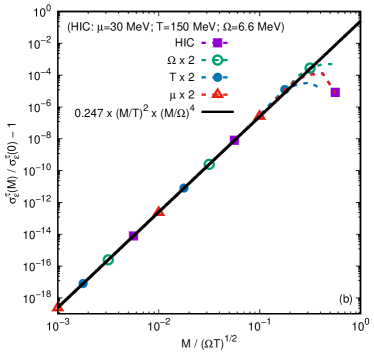
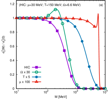
Figure 10: (a) Relative mass correction $\sigma_{\varepsilon}^{\tau}(M)/\sigma_{\varepsilon}^{\tau}(0)-1$, represented with respect to $x=M/\sqrt{T\Omega}$. The solid black line represents the best fit curve of the function $\alpha x^{4}$. (b) Ratio $\sigma_{\varepsilon}^{\tau}(M)/\sigma_{\varepsilon}^{\tau}(0)$, represented with respect to $M$ for various parameter choices.

Turning to the circular heat conductivity $\sigma_{\varepsilon}^{\tau}$, whose massless limit is given in Eq. (221), Fig. 10(a) confirms that the leading order mass correction, computed as $\sigma_{\varepsilon}^{\tau}(M)/\sigma_{\varepsilon}^{\tau}(0)-1$, is of order $O(M^{4})$. Fig. 10(b) confirms the validity of the constitutive relation for massess up to $\sim 100\ {\rm MeV}$ for the HIC values of $\mu$, $T$ and $\Omega$. The spike seen when $M\rightarrow\mu$ at large $\mu$ is akin to the one observed for $\Delta Q_{\pm}$, $\sigma^{\tau}_{\pm}$ and $\Delta E$ in Figs. 2(c), 2(d) and 9(c). The peak observed in the curve corresponding to $\Omega\simeq 2\ {\rm GeV}$ is akin to the one observed for the axial vortical conductivity $\sigma^{\omega}_{A}$ in Fig. 5(b).

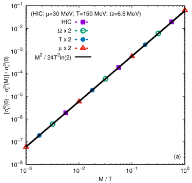
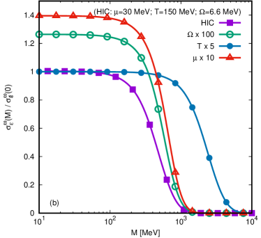
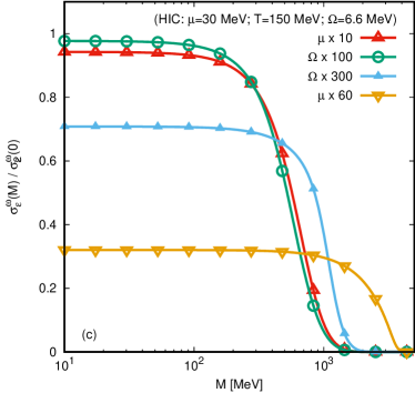
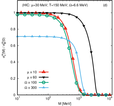
Figure 11: (a) Relative mass correction $1-\sigma_{\varepsilon}^{\omega}(M)/\sigma_{\varepsilon}^{\omega}(0)$, represented with respect to $M/T$. The solid black line represents the prediction given in Eq. (220). (b)-(d) Ratio $\sigma_{\varepsilon}^{\omega}(M)/\sigma_{\varepsilon}^{\omega;n}(0)$ between $\sigma_{\varepsilon}^{\omega}(M)$ computed using Eq. (219) and the approximations $\sigma_{\varepsilon}^{\omega;n}(0)$ given in Eqs. (222), (223) and (224) for (b) $n=1$, (c) $n=2$ and (d) $n=3$.

The heat conductivity $\sigma_{\varepsilon}^{\omega}$ along the vector $\omega^{\hat{\alpha}}$ is considered in Fig. 11. This quantity can be obtained in closed form on the rotation axis, for any mass, and is given in terms of the polylogarithm functions in Eq. (219). First, the leading order contribution coming from the mass is considered. Figure 11(a) presents the relative mass correction, $1-\sigma_{\varepsilon}^{\omega}(M)/\sigma_{\varepsilon}^{\omega}(0)$, with respect to the ratio $M/T$. The second order contribution predicted in Eqs. (214) and (220) is confirmed.

The expression for $\sigma_{\varepsilon}^{\omega}$ derived in Eq. (219) is valid only on the rotation axis and is thus inapplicable for studying the properties of $\sigma_{\varepsilon}^{\omega}$, e.g., in the vicinity of the speed of light surface, as well as the interplay between the vorticity $\omega^{\hat{z}}=\Omega\Gamma^{2}$ and acceleration $a^{\hat{\rho}}=-\rho\Omega\Gamma^{2}$, since the latter vanishes on the rotation axis. Another drawback concerns the complexity of the polylogarithm functions, which make the physical properties of $\sigma_{\varepsilon}^{\omega}$ difficult to assess. To this end, three levels of approximations are employed, following the approach taken for $\sigma^{\omega}_{\pm}(M)$ and $Q_{A}(M)$, which are represented in Figs. 4(b-d) and 6(b-d), respectively. The approximations are denoted using $\sigma_{\varepsilon}^{\omega;n}$, with $1\leq n\leq 3$, and are based on Eq. (213). The cases $n=1$ and $n=2$ are obtained from the high temperature expansion given in Eq. (214). For the $n=1$ term, only the leading order contribution is taken into account:

$$\sigma_{\varepsilon}^{\omega;1}=\frac{4\mu_{H}\mu_{V}T}{\pi^{2}}\ln 2.$$ (222)

As can be seen in Fig. 11(b), this approximation works well for the HIC parameters, breaking down when $M\gtrsim T$. This is confirmed by looking at the curve corresponding to $T\simeq 750\ {\rm MeV}$ (blue line and solid circles). However, the results for higher vorticity ($\Omega=660\ {\rm MeV}$ for the green line and empty circles) and higher chemical potential ($\mu=300\ {\rm MeV}$ for the red line and empty triangles) show a discrepancy.

The $n=2$ approximation takes into account the $T^{-1}$ correction appearing in Eq. (214), but disregards the mass term:

$$\sigma_{\varepsilon}^{\omega;2}=\frac{4\mu_{H}\mu_{V}T}{\pi^{2}}\ln 2+\frac{\mu_{H}\mu_{V}}{6\pi^{2}T}\left(\mu_{H}^{2}+\mu_{V}^{2}+\frac{\bm{\omega}^{2}+\bm{a}^{2}}{4}\right).$$ (223)

It should be noted that on the rotation axis, Eq. (223) coincides with the massless limit of Eq. (220), which represents the high temperature expansion of the exact result in Eq. (219). Figure 11(c) shows that this second approximation works well for the two problematic cases discussed in Fig. 11(b), i.e., $\Omega=660\ {\rm MeV}$ and $\mu=300\ {\rm MeV}$. Further increasing the vorticity ($\Omega\simeq 2\ {\rm GeV}$ for the blue line with filled upper triangles) or the chemical potential ($\mu=0.9\ {\rm GeV}$ for the orange line and lower, filled triangles) again gives rise to discrepancies. The final approximation considered here is obtained by setting $M=0$ in Eq. (213):

$$\sigma_{\varepsilon}^{\omega;3}=-\frac{T^{3}}{\pi^{2}}\left[{\rm Li}_{3}(-e^{-\mu_{+}/T})-{\rm Li}_{3}(-e^{-\mu_{-}/T})-{\rm Li}_{3}(-e^{\mu_{+}/T})+{\rm Li}_{3}(-e^{\mu_{-}/T})\right]\\ +\frac{T}{12\pi^{2}}(\bm{\omega}^{2}+\bm{a}^{2})\ln\left[\frac{\cosh\frac{1}{2T}(\mu_{V}+\mu_{H})}{\cosh\frac{1}{2T}(\mu_{V}-\mu_{H})}\right].$$ (224)

Fig. 11(d) shows that this approximation works well at high chemical potential, however, the discrepancy at $\Omega=2\ {\rm GeV}$ remains similar to that seen in Fig. 11(c). This discrepancy is due to the fact that Eq. (213) represents a small $\Omega$ expansion which is valid only up to second order in $\Omega$.

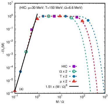
Figure 12: Dependence of $\Pi_{1}(M)$ on the ratio $M/\Omega$ for various values of the parameters. The solid black line shows the best fit of the expression $\alpha(M/\Omega)^{6}$ to the numerical data.

In the case of the coefficient $\Pi_{1}$, the analysis in the previous subsection indicated that $\Pi_{1}$ vanishes up to $O(M^{4})$. Fig. 12 shows that the leading order contribution to $\Pi_{1}$ is of order $(M/\Omega)^{6}$.

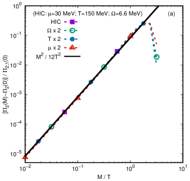
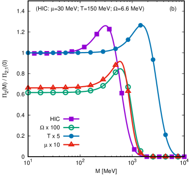
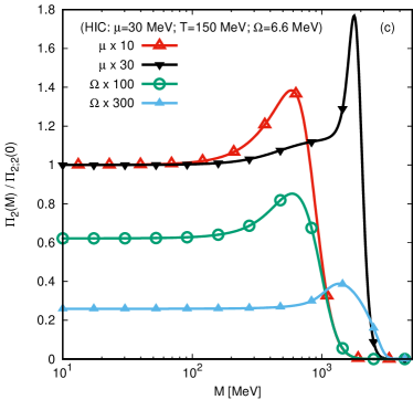
Figure 13: (a) Relative mass correction $[\Pi_{2}(M)-\Pi_{2}(0)]/\Pi_{2;1}$, represented with respect to $M/T$. The solid black line represents the prediction given in Eq. (220). (b)-(c) Ratios $\Pi_{2}(M)/\Pi_{2;n}(0)$ between $\Pi_{2}(M)$ computed using Eq. (219) and the approximations $\Pi_{2;n}(0)$ given in Eqs. (225) and (226) for (b) $n=1$ and (c) $n=2$, respectively.

In the case of $\Pi_{2}$, the same situation as for $\sigma_{\varepsilon}^{\omega}$ is encountered: Eq. (219) gives the exact value of $\Pi_{2}$ on the rotation axis, for any mass, while Eq. (213) gives its value up to $O(\Omega^{2})$ for any value of $\rho$. The mass is predicted through Eqs. (214) and (220) to contribute a correction of order $O(M^{2})$. This is confirmed in Fig. 13(a). Next, the high temperature approximation given in Eq. (214) is considered, which is labelled according to the convention in this section as $\Pi_{2;1}$:

$$\Pi_{2;1}=-\frac{\mu_{H}\mu_{V}}{6\pi^{2}T}.$$ (225)

As demonstrated in Fig. 13(b), this approximation is valid for the HIC conditions, but loses applicability when either $\Omega$ or $\mu$ are increased. The second approximation is the one derived in Eq. (213), which is valid up to $O(\Omega^{2})$:

$$\Pi_{2;2}=-\frac{T}{3\pi^{2}}\ln\left[\frac{\cosh\frac{\beta}{2}(\mu_{V}+\mu_{H})}{\cosh\frac{\beta}{2}(\mu_{V}-\mu_{H})}\right]+O(\Omega^{2},M^{2}).$$ (226)

Fig. 13(c) shows that this approximation is valid at high values of the chemical potential ($\mu=0.9\ {\rm GeV}$ is shown with black lines and lower, filled triangles), but remains inaccurate at high vorticities. This is because Eq. (213) is derived as a small $\Omega$ expansion, which can be expected to be inaccurate at high values of $\Omega$.

10 Conclusions

		Leading order	Reference
$J^{\mu}_{V/H}$	$\sigma^{\tau}_{V/H}$	$\dfrac{\mu_{V/H}}{6\pi^{2}}+O(M^{4})$	(127)
	$\sigma^{\omega}_{V/H}$	$\dfrac{2\mu_{H/V}T}{\pi^{2}}\ln 2+O(T^{-1})$	(131), (138)
$J^{\mu}_{A}$	$\sigma^{\tau}_{A}$	$\dfrac{\mu_{V}\mu_{H}}{12\pi^{2}T}\left(1-\dfrac{4M^{2}}{\Omega^{2}}\right)+O(T^{-2})$	(166), (172)
	$\sigma^{\omega}_{A}$	$\dfrac{T^{2}}{6}+\dfrac{\mu_{V}^{2}+\mu_{H}^{2}}{2\pi^{2}}+O(M^{4})$	(160)
$T^{\mu\nu}$	$\sigma_{\varepsilon}^{\tau}$	$-\dfrac{T^{2}}{18}-\dfrac{\mu_{V}^{2}+\mu_{H}^{2}}{6\pi^{2}}+O(M^{4})$	(209)
	$\sigma_{\varepsilon}^{\omega}$	$\dfrac{4\mu_{V}\mu_{H}T}{\pi^{2}}\ln 2+O(T{{}^{-}1})$	(213),(219)
	$\Pi_{1}$	$O(M^{4})$	(209)
	$\Pi_{2}$	$\dfrac{4\mu_{V}\mu_{H}T}{\pi^{2}}\ln 2+O(T^{-1})$	(213),(219)

Table 1: Summary of the anomalous transport coefficients for the vector/helical charge currents $J^{\mu}_{V/H}$, axial current $J^{\mu}_{A}$ and stress-energy tensor $T^{\mu\nu}$. Only the leading order terms are shown in this table. Higher order terms can be found in the equations given as references. When a second equation is provided, it gives the exact value of the corresponding quantity on the rotation axis.

In this paper, the properties of massive Dirac fermions under rotation at finite temperature and finite chemical potential were considered. Aside from the chemical potential associated to the vector charge ($\mu_{V}$), a helicity chemical potential ($\mu_{H}$) accounting for the polarisation imbalance was taken into account. A simple relativistic kinetic theory (RKT) model incorporating the helicity imbalance was proposed to serve as a background classical theory. Within this kinetic framework, the vector and helicity charge currents (VCC and HCC) and the stress-energy tensor (SET) have the form corresponding to the perfect fluid, being characterised by the charge densities $Q^{\rm RKT}_{V}$ and $Q^{\rm RKT}_{H}$, energy density $E_{\rm RKT}$ and pressure $P_{\rm RKT}$.

The quantum thermal expectation values (t.e.v.s) were computed by performing an exact trace over Fock space using the mode basis introduced in Refs. ambrus14plb ; ambrus16prd ; ambrus19lnp with respect to which the thermal weight function ${\hat{\varrho}}$ is diagonal. For all quantities involved, a small mass expansion was derived analytically, valid at any distance between the rotation axis and the speed of light surface (SLS). Compared to the RKT results, the quantum t.e.v.s exhibit corrections at the level of $Q_{V}$, $Q_{H}$, $E$ and $P$, which are proportional to the square of the vorticity ($\bm{\omega}^{2}=\Omega^{2}\Gamma^{4}$) or of the acceleration [$\bm{a}^{2}=\Omega^{2}\Gamma^{2}(\Gamma^{2}-1)$]. Furthermore, the anomalous contributions to the charge currents and SET were highlighted. The corresponding transport coefficients are summarised to leading order for convenience in Table 1. The results derived in this paper agree in the massless limit with the vanishing axial chemical potential ($\mu_{A}$) limit of the results derived in Refs. helican and buzzegoli18 (the $\mu_{H}\rightarrow 0$ limit is necessary to compare with the latter reference).

It was shown that, under the conditions which are prevalent in the quark-gluon plasma formed in relativistic heavy ion collisions experiments (the HIC conditions), the constitutive relations are in general robust, in the sense that they remain valid for masses up to the thermal energy ($M\lesssim 150\ {\rm MeV}$). The only exception was seen in the case of the circular axial charge conductivity $\sigma_{A}^{\tau}$, which exhibits a peculiar mass dependence of the form $M^{2}/\Omega^{2}$. The mass correction $\delta\sigma_{A}^{\tau}=\sigma_{A}^{\tau}(M)-\sigma_{A}^{\tau}(0)$ becomes dominant over the massless value when $M\simeq\Omega$.

As pointed out in Sec. 3.3, the transport laws involving the helicity chemical potential $\mu_{H}$ strongly suggest a new type of anomalies in quantum electrodynamics (QED), which may be investigated by considering the $AHH$ and $HTV$ triangle diagrams, involving vector ($V$), axial ($A$), helical ($H$) and graviton ($T$) vertices.

Appendix A Fermi-Dirac integration formulae

In this section, the procedure for computing the integrals involving the Fermi-Dirac distribution function for massless particles appearing in the relativistic kinetic theory (RKT) formulation discussed in Sec. 4 and in the quantum field theory (QFT) formulation discussed in Sections 6–9 is presented.

The first set of integrals that will be discussed can be introduced as follows:

$$I^{-}_{n}(a)= \frac{1}{2}\int_{0}^{\infty}dx\,x^{2n}\left(\frac{1}{e^{x-a}+1}-\frac{1}{e^{x+a}+1}\right),$$

$$I^{+}_{n}(a)= \frac{1}{2}\int_{0}^{\infty}dx\,x^{2n+1}\left(\frac{1}{e^{x-a}+1}+\frac{1}{e^{x+a}+1}\right).$$ (227)

An expansion of the Fermi-Dirac factors in powers of $a$ can be considered, as follows:

$$\frac{1}{e^{x\pm a}+1}=\sum_{j=0}^{\infty}\frac{(\pm a)^{j}}{j!}\frac{d^{j}}{dx^{j}}\left(\frac{1}{e^{x}+1}\right).$$ (228)

Inserting this expansion in Eq. (227) gives:

$$I^{-}_{n}(a)= -\int_{0}^{\infty}dx\,x^{2n}\sum_{j=0}^{\infty}\frac{a^{2j+1}}{(2j+1)!}\frac{d^{2j+1}}{dx^{2j+1}}\left(\frac{1}{e^{x}+1}\right),$$

$$I^{+}_{n}(a)= \int_{0}^{\infty}dx\,x^{2n+1}\sum_{j=0}^{\infty}\frac{a^{2j}}{(2j)!}\frac{d^{2j}}{dx^{2j}}\left(\frac{1}{e^{x}+1}\right).$$ (229)

It can now be assumed that the summation and integration signs can be interchanged. This assumption will prove to be justified by the structure of the result. Integration by parts can be performed in the above expressions, yielding:

$$I^{-}_{n}= \sum_{j=0}^{n-1}\binom{2n}{2j+1}a^{2j+1}\int_{0}^{\infty}dx\frac{x^{2n-2j-1}}{e^{x}+1}-\sum_{j=0}^{\infty}\frac{a^{2n+2j+1}(2n)!}{(2n+2j+1)!}\int_{0}^{\infty}dx\,\frac{d^{2j+1}}{dx^{2j+1}}\left(\frac{1}{e^{x}+1}\right),$$

$$I^{+}_{n}= \sum_{j=0}^{n}\binom{2n+1}{2j}a^{2j}\int_{0}^{\infty}dx\frac{x^{2n+1-2j}}{e^{x}+1}-\sum_{j=0}^{\infty}\frac{a^{2(n+j+1)}(2n+1)!}{(2n+2j+2)!}\int_{0}^{\infty}dx\,\frac{d^{2j+1}}{dx^{2j+1}}\left(\frac{1}{e^{x}+1}\right),$$ (230)

where the explicit dependence of $I^{\pm}_{n}$ on $a$ was dropped for brevity. The second terms appearing above can be integrated, yielding:

$$\int_{0}^{\infty}dx\,\frac{d^{2j+1}}{dx^{2j+1}}\left(\frac{1}{e^{x}+1}\right)=-\frac{d^{2j}}{dx^{2j}}\left.\left(\frac{1}{e^{x}+1}\right)\right\rfloor_{x=0}.$$ (231)

Noting that

$$\frac{1}{e^{x}+1}+\frac{1}{e^{-x}+1}=\frac{1}{2},$$ (232)

it can be seen that $(e^{x}+1)^{-1}$ admits the following series representation about $x=0$:

$$\frac{1}{e^{x}+1}=\frac{1}{2}+\sum_{\ell=0}^{\infty}\frac{a_{\ell}}{(2\ell+1)!}x^{2\ell+1},$$ (233)

where the exact expression for $a_{\ell}$ is not important. The only even term in the series (233) is the leading $1/2$, while all other terms are odd with respect to $x$. Thus, Eq. (231) is non-vanishing only when $j=0$, such that:

$$\int_{0}^{\infty}dx\,\frac{d^{2j+1}}{dx^{2j+1}}\left(\frac{1}{e^{x}+1}\right)=\begin{cases}-\frac{1}{2},&j=0,\\ 0,&\text{ otherwise.}\end{cases}$$ (234)

Thus, Eq. (230) reduces to:

$$I^{-}_{n}(a)= \sum_{j=0}^{n-1}\binom{2n}{2j+1}a^{2j+1}\int_{0}^{\infty}dx\frac{x^{2n-2j-1}}{e^{x}+1}+\frac{a^{2n+1}}{2(2n+1)},$$

$$I^{+}_{n}(a)= \sum_{j=0}^{n}\binom{2n+1}{2j}a^{2j}\int_{0}^{\infty}dx\frac{x^{2n+1-2j}}{e^{x}+1}+\frac{a^{2(n+1)}}{4(n+1)}.$$ (235)

The terms in the sums appearing in Eq. (235) are standard Fermi-Dirac integrals. The first few of these integrals can be computed exactly:

$$\int_{0}^{\infty}\frac{x\,dx}{e^{x}+1}=\frac{\pi^{2}}{12},\qquad\int_{0}^{\infty}\frac{x^{3}dx}{e^{x}+1}=\frac{7\pi^{4}}{120}.$$ (236)

Thus, the following results can be obtained:

$$I^{-}_{0}(a)=\frac{a}{2},\qquad I^{-}_{1}(a)=\frac{a\pi^{2}}{6}+\frac{a^{3}}{6},\qquad I^{-}_{2}(a)=\frac{7a\pi^{4}}{30}+\frac{a^{3}\pi^{2}}{3}+\frac{a^{5}}{10},$$

$$I^{+}_{0}(a)=\frac{\pi^{2}}{12}+\frac{a^{2}}{4},\qquad I^{+}_{1}(a)=\frac{7\pi^{4}}{120}+\frac{\pi^{2}a^{2}}{4}+\frac{a^{4}}{8}.$$ (237)

Aside from the integrals $I_{n}^{\pm}(a)$ considered in Eq. (227), the analysis in the main text requires the computation of integrals when the subscript of $I$ is no longer an integer. Retaining the convention that $n=0,1,2,\dots$ is a natural number, the integrals $I_{n+1/2}^{\pm}(a)$ can be defined by analogy to Eq. (227) as follows:

$$I^{-}_{n+1/2}(a)= \frac{1}{2}\int_{0}^{\infty}dx\,x^{2n+1}\left(\frac{1}{e^{x-a}+1}-\frac{1}{e^{x+a}+1}\right),$$

$$I^{+}_{n+1/2}(a)= \frac{1}{2}\int_{0}^{\infty}dx\,x^{2n+2}\left(\frac{1}{e^{x-a}+1}+\frac{1}{e^{x+a}+1}\right).$$ (238)

The equivalent of Eq. (230) becomes:

$$I^{-}_{n+1/2}= \sum_{j=0}^{n}\binom{2n+1}{2j+1}a^{2j+1}\int_{0}^{\infty}dx\frac{x^{2n-2j}}{e^{x}+1}-\sum_{j=0}^{\infty}\frac{a^{2n+2j+3}(2n+1)!}{(2n+2j+3)!}\frac{d^{2j+1}}{dx^{2j+1}}\left(\frac{1}{e^{x}+1}\right)_{x=0},$$

$$I^{+}_{n-1/2}= \sum_{j=0}^{n}\binom{2n}{2j}a^{2j}\int_{0}^{\infty}dx\frac{x^{2n-2j}}{e^{x}+1}-\sum_{j=0}^{\infty}\frac{a^{2(n+j+1)}(2n)!}{(2n+2j+2)!}\frac{d^{2j+1}}{dx^{2j+1}}\left(\frac{1}{e^{x}+1}\right)_{x=0},$$ (239)

where the arguments $a$ were dropped for brevity. The integration with respect to $x$ can be performed in terms of the zeta function:

$$\int_{0}^{\infty}\frac{dx\,x^{2n-2j}}{e^{x}+1}=(1-4^{j-n})(2n-2j)!\zeta(2n+1-2j),$$ (240)

where the case $n=j$ is obtained via the following limit:

$$\lim_{\nu\rightarrow 0}(1-4^{\nu})\Gamma(1-2\nu)\zeta(1-2\nu)=\ln 2.$$ (241)

For the second sum over $j$ in Eq. (239), it is useful to note that:

$$-\sum_{j=0}^{\infty}\frac{a^{2j+k+1}}{(2j+k+1)!}\frac{d^{2j+1}}{dx^{2j+1}}\left(\frac{1}{e^{x}+1}\right)_{x=0}=\frac{1}{2}\sum_{j=0}^{\infty}\frac{a^{j+k}}{(j+k)!}\frac{d^{j}}{dx^{j}}\left(\tanh\frac{x}{2}\right)_{x=0},$$ (242)

where $\tanh\frac{x}{2}=(e^{-x}+1)^{-1}-(e^{x}+1)^{-1}$, while $k=2n+2$ for $I_{n+1/2}^{-}$ and $k=2n+1$ for $I_{n-1/2}^{+}$. The summation can be interpreted as a Maclaurin series by noting that

$$\frac{a^{j+k}}{(j+k)!}=\int_{0}^{a}da_{1}\int_{0}^{a_{1}}da_{2}\dots\int_{0}^{a_{k-1}}da_{k}\frac{a_{k}^{j}}{j!}.$$ (243)

Using the relation:

$$\sum_{j=0}^{\infty}\frac{a^{j}}{j!}\frac{d^{j}}{dx^{j}}\left(\tanh\frac{x}{2}\right)_{x=0}=\tanh\frac{a}{2},$$ (244)

the following results can be obtained:

$$I^{-}_{n+1/2}(a)= \sum_{j=0}^{n}\frac{(2n+1)!}{(2j+1)!}a^{2j+1}(1-4^{j-n})\zeta(2n+1-2j)$$

$$+2^{2n+1}(2n+1)!\int_{0}^{\frac{a}{2}}da_{1}\dots\int_{0}^{a_{2n+1}}da_{2n+2}\tanh a_{2n+2},$$

$$I^{+}_{n-1/2}(a)= \sum_{j=0}^{n}\frac{(2n)!}{(2j)!}a^{2j}(1-4^{j-n})\zeta(2n+1-2j)$$

$$+2^{2n}(2n)!\int_{0}^{\frac{a}{2}}da_{1}\dots\int_{0}^{a_{2n}}da_{2n+1}\tanh a_{2n+1}.$$ (245)

For small values of $n$, Eq. (245) reduces to:

$$I^{-}_{1/2}(a)=\frac{1}{2}[{\rm Li}_{2}(-e^{-a})-{\rm Li}_{2}(-e^{a})],\qquad I^{-}_{3/2}(a)=3[{\rm Li}_{4}(-e^{-a})-{\rm Li}_{4}(-e^{a})],$$

$$I^{+}_{-1/2}(a)=\ln\left(2\cosh\frac{a}{2}\right),\qquad I^{+}_{1/2}(a)=-{\rm Li}_{3}(-e^{-a})-{\rm Li}_{3}(-e^{a}),$$

$$I^{+}_{3/2}(a)=-12[{\rm Li}_{5}(-e^{-a})+{\rm Li}_{5}(-e^{a})],$$ (246)

where ${\rm Li}_{n}(z)=\sum_{k=1}^{\infty}z^{k}/n^{k}$ is the polylogarithm. The following relations were employed:

$$\int_{0}^{a}dx\,\tanh x=\ln\cosh a,\qquad\int_{0}^{a}dx\,\ln\cosh x=\frac{a^{2}}{2}-a\ln 2+\frac{\pi^{2}}{24}+\frac{1}{2}{\rm Li}_{2}(-e^{-2a}),$$

$$\int_{0}^{a}dx\,{\rm Li}_{n}(-e^{-2x})=-\frac{1}{2}(1-2^{-n})\zeta(n+1)-\frac{1}{2}{\rm Li}_{n+1}(-e^{-2a}).$$ (247)

For future convenience, the following properties of the polylogarithm are listed below:

$${\rm Li}_{2}(-e^{-a})+{\rm Li}_{2}(-e^{a})= -\frac{\pi^{2}}{6}-\frac{a^{2}}{2},$$

$${\rm Li}_{3}(-e^{-a})-{\rm Li}_{3}(-e^{a})= \frac{\pi^{2}a}{6}+\frac{a^{3}}{6},$$

$${\rm Li}_{4}(-e^{-a})+{\rm Li}_{4}(-e^{a})= --\frac{7\pi^{4}}{360}-\frac{\pi^{2}a^{2}}{12}-\frac{a^{4}}{24},$$

$${\rm Li}_{5}(-e^{-a})-{\rm Li}_{5}(-e^{a})= \frac{7\pi^{4}a}{360}+\frac{\pi^{2}a^{3}}{36}+\frac{a^{5}}{120}.$$ (248)

References

- (1) A. Vilenkin, Parity nonconservation and rotating black holes, Phys. Rev. Lett. 41 (1978) 1575.
- (2) STAR collaboration, Global hyperon polarization in nuclear collisions, Nature 548 (2017) 62.
- (3) STAR collaboration, Global polarization of hyperons in AuAu collisions at , Phys. Rev. C 98 (2018) 014910.
- (4) D. E. Kharzeev, J. Liao, S. A. Voloshin and G. Wang, Chiral magnetic and vortical effects in high-energy nuclear collisions - A status report, Prog. Part. Nucl. Phys. 88 (2016) 1.
- (5) O. V. Rogachevsky, A. S. Sorin and O. V. Teryaev, Chiral vortaic effect and neutron asymmetries in heavy-ion collisions, Phys. Rev. C 82 (2010) 054910.
- (6) M. Baznat, K. Gudima, A. Sorin and O. Teryaev, Helicity separation in heavy-ion collisions, Phys. Rev. C 88 (2013) 061901(R).
- (7) M. Baznat, K. Gudima, A. Sorin and O. Teryaev, Hyperon polarization in heavy-ion collisions and holographic gravitational anomaly, Phys. Rev. C 97 (2018) 041902(R).
- (8) K. Fukushima, D. E. Kharzeev and H. J. Warringa, Chiral magnetic effect, Phys. Rev. D 78 (2008) 074033.
- (9) V. Braguta, M. N. Chernodub, V. A. Goy, K. Landsteiner, A. V. Molochkov and M. I. Polikarpov, Temperature dependence of the axial magnetic effect in two-color quenched QCD, Phys. Rev. D 89 (2014) 074510.
- (10) M. Buzzegoli and F. Becattini, General thermodynamic equilibrium with axial chemical potential for the free Dirac field, Journal of High Energy Physics 2018 (2018) 2.
- (11) F. Becattini, W. Florkowski and E. Speranza, Spin tensor and its role in non-equilibrium thermodynamics, Phys. Lett. B 789 (2019) 419.
- (12) V. E. Ambru\cbs and M. Chernodub, Helical vortical effects, helical waves and anomalies of Dirac fermions, arXiv:1912.11034 [hep-th] (2019) .
- (13) C. Pozrikidis, The fractional Laplacian. CRC Press, Boca Raton, FL, 2016.
- (14) C. Itzykson and J.-B. Zuber, Quantum field theory. Dover, 1980.
- (15) S. Weinberg, The Quantum theory of fields. Vol. I: Foundations. Cambridge University Press, 1995.
- (16) M. E. Peskin and D. V. Schroeder, An introduction to quantum field theory. Addison-Wesley Publishing Company, 1995.
- (17) S. J. Brodsky and G. P. Lepage, Exclusive processes in quantum chromodynamics, in Perturbative quantum chromodynamics (advanced series on directions in high energy physics, Vol 5), A. H. Mueller, ed., (Singapore), pp. 93–240, World Scientific, (1989).
- (18) J. I. Kapusta, E. Rrapaj and S. Rudaz, Spin versus helicity equilibration times and Lagrangian for strange quarks in rotating quark-gluon plasma, arXiv:2004.14807 [hep-th] (2020) .
- (19) M. Ruggieri, G. X. Peng and M. Chernodub, Chiral relaxation time at the crossover of quantum chromodynamics, Phys. Rev. D 94 (2016) 054011.
- (20) J. I. Kapusta, E. Rrapaj and S. Rudaz, Hyperon polarization in relativistic heavy ion collisions and axial U(1) symmetry breaking at high temperature, Phys. Rev. C 101 (2020) 031901.
- (21) M. Ruggieri, M. N. Chernodub and Z.-Y. Lu, Topological susceptibility, divergent chiral density and phase diagram of chirally imbalanced qcd medium at finite temperature, arXiv:2004.09393 [hep-ph] (2020) .
- (22) A. Vilenkin, Quantum field theory at finite temperature in a rotating system, Phys. Rev. D 21 (1980) 2260.
- (23) J. I. Kapusta and P. V. Landshoff, Finite-temperature field theory, J. Phys. G: Nucl. Part. Phys. 15 (1989) 267.
- (24) M. Laine and A. Vuorinen, Basics of thermal field theory. Springer, 2016.
- (25) S. Mallik and S. Sarkar, Hadrons at finite temperature. Cambridge University Press, 2016.
- (26) D. N. Zubarev, A. V. Prozorkevich and S. Smolyanskii, Derivation of nonlinear generalized equations of quantum hydrodynamics, Theoret. Math. Phys. 40 (1979) 821.
- (27) F. Becattini and E. Grossi, Quantum corrections to the stress-energy tensor in thermodynamic equilibrium with acceleration, Phys. Rev. D 92 (2015) 045037.
- (28) M. Buzzegoli, Thermodynamic equilibrium of massless fermions with vorticity, chirality and magnetic field, Ph.D. thesis, Universita degli studi Firenze, 2020.
- (29) M. Casals, S. R. Dolan, B. C. Nolan, A. Ottewill and E. Winstanley, Quantization of fermions on Kerr space-time, Phys. Rev. D 87 (2013) 064027.
- (30) V. E. Ambru\cbs and E. Winstanley, Rotating quantum states, Phys. Lett. B 734 (2014) 296.
- (31) N. D. Birrell and P. C. W. Davies, Quantum fields in curved space. Cambridge University Press, 1982.
- (32) G. Duffy and A. C. Ottewill, Rotating quantum thermal distribution, Phys. Rev. D 67 (2003) 044002.
- (33) R. Panerai, Global equilibrium and local thermodynamics in stationary spacetimes, Phys. Rev. D 93 (2016) 104021.
- (34) V. E. Ambru\cbs and E. Winstanley, Rotating fermions inside a cylindrical boundary, Phys. Rev. D 93 (2016) 104014.
- (35) S. Jeon, Hydrodynamic transport coefficients in relativistic scalar field theory, Phys. Rev. D 52 (1995) 3591.
- (36) D. E. Kharzeev and H. J. Warringa, Chiral magnetic conductivity, Phys. Rev. D 80 (2009) 034028.
- (37) K. Landsteiner, E. Megías and F. Pena-Benitez, Gravitational anomaly and transport phenomena, Phys. Rev. Lett. 107 (2011) 021601.
- (38) J. Schwinger, Brownian motion of a quantum oscillator, J. Math. Phys. 2 (1961) 407.
- (39) L. V. Keldysh, Diagram technique for nonequilibrium processes, Sov. Phys. JETP 20 (1965) 1018.
- (40) P. Danielewicz, Quantum theory of nonequilibrium processes, i, Sov. Phys. JETP 20 (2018) 1018.
- (41) K. Landsteiner, E. Megías and F. Pena-Benitez, Anomalous transport from kubo formulae, in Strongly interacting matter in magnetic fields (Lecture notes in physics 871), D. Kharzeev, K. Landsteiner, A. Schmitt and H.-U. Yee, eds., (Berlin Heidelberg), pp. 433–468, Springer-Verlag, (2013).
- (42) Y. Jiang and J. Liao, Pairing phase transition of matter under rotation, Phys. Rev. Lett. 117 (2016) 192302.
- (43) S. Ebihara, K. Fukushima and K. Mameda, Boundary effects and gapped dispersion in rotating fermionic matter, Phys. Lett. B 764 (2017) 94.
- (44) M. N. Chernodub and S. Gongyo, Effects of rotation and boundaries on chiral symmetry breaking of relativistic fermions, Phys. Rev. D 95 (2017) 096006.
- (45) M. N. Chernodub and S. Gongyo, Edge states and thermodynamics of rotating relativistic fermions under magnetic field, Phys. Rev. D 96 (2017) 096014.
- (46) V. E. Ambru\cbs and E. Winstanley, Exact solutions in quantum field theory under rotation, in Strongly Interacting Matter under Rotation, F. Becattini, J. Liao and M. Lisa, eds., (Under review), arXiv:1908.10244 [hep-th], (2019).
- (47) B. R. Iyer, Dirac field theory in rotating coordinates, Phys. Rev. D 26 (1982) 1900.
- (48) J. R. Letaw and J. D. Pfautsch, Quantized scalar field in rotating coordinates, Phys. Rev. D 22 (1980) 1345.
- (49) J. R. Letaw and J. D. Pfautsch, Quantized scalar field in the stationary coordinate systems of flat spacetime, Phys. Rev. D 24 (1981) 1491.
- (50) B. S. Kay and R. M. Wald, Theorems on the uniqueness and thermal properties of stationary, nonsingular, quasifree states on spacetimes with a bifurcate Killing horizon, Phys. Rep. 207 (1991) 49.
- (51) A. C. Ottewill and E. Winstanley, Renormalized stress tensor in kerr space-time: General results, Phys. Rev. D 62 (2000) 084018.
- (52) A. C. Ottewill and E. Winstanley, Divergence of a quantum thermal state on kerr space-time, Phys. Lett. A 273 (2000) 149.
- (53) A. Vilenkin, Macroscopic parity-violating effect: Neutrino fluxes from rotating black holes and in rotating thermal radiation, Phys. Rev. D 20 (1979) 1807.
- (54) N. Nicolaevici, Null response of uniformly rotating unruh detectors in bounded regions, Class. Quantum Grav. 18 (2001) 5407.
- (55) V. E. Ambru\cbs and I. I. Cotăescu, Maxwell-Jüttner distribution for rigidly-rotating flows in spherically symmetric spacetimes using the tetrad formalism, Phys. Rev. D 94 (2016) 085022.
- (56) V. E. Ambru\cbs, Fermion condensation under rotation on anti-de sitter space, arXiv:1912.02014 [hep-th] (2019) .
- (57) P. Ván and T. S. Biró, First order and stable relativistic dissipative hydrodynamics, Phys. Lett. B 709 (2012) 106.
- (58) P. Ván and T. S. Biró, Dissipation flow-frames: particle, energy, thermometer, in Proceedings of the 12th Joint European Thermodynamics Conference, M. Pilotelli and G. P. Beretta, eds., pp. 546–551, (2013).
- (59) F. Becattini, L. Bucciantini, E. Grossi and L. Tinti, Local thermodynamical equilibrium and the -frame for a quantum relativistic fluid, Eur. Phys. J C 75 (2015) 191.
- (60) K. Landsteiner, E. Megías, L. Melgar and F. Pena-Benitez, Holographic gravitational anomaly and chiral vortical effect, JHEP 09 (2011) 121.
- (61) V. E. Ambru\cbs, Quantum non-equilibrium effects in rigidly-rotating thermal states, Phys. Lett. B 771 (2017) 151.
- (62) B. V. Jacak and B. Muller, The exploration of hot nuclear matter, Science 337 (2012) 310.
- (63) X.-G. Huang and T. Koide, Shear viscosity, bulk viscosity, and relaxation times of causal dissipative relativistic fluid-dynamics at finite temperature and chemical potential, Nucl. Phys. A 889 (2012) 73.
- (64) Q. Wang, Global and local spin polarization in heavy ion collisions: a brief overview, Nucl. Phys. A 967 (2017) 225.
- (65) W. A. Bardeen, Anomalous Ward identities in spinor field theories, Phys. Rev. 184 (1969) 1848.
- (66) R. A. Bertlmann, Anomalies in quantum field theroy. Clarendon Press, Oxford, UK, 1996.
- (67) C. Cercignani and G. M. Kremer, The relativistic Boltzmann equation: theory and applications. Birkhäuser Verlag, Basel, Switzerland, 2002.
- (68) S. R. de Groot, W. A. van Leeuwen and C. G. van Weert, Relativistic kinetic theory: principles and applications. North Holland, 1980.
- (69) F. Becattini, V. Chandra, L. D. Zanna and E. Grossi, Relativistic distribution function for particles with spin at local thermodynamical equilibrium, Ann. Phys. 338 (2013) 32.
- (70) W. Florkowski, B. Friman, A. Jaiswal and E. Speranza, Relativistic fluid dynamics with spin, Phys. Rev. C 97 (2018) 041901(R).
- (71) W. Florkowski, A. Kumar and R. Ryblewski, Thermodynamic versus kinetic approach to polarization-vorticity coupling, Phys. Rev. C 98 (2018) 044906.
- (72) N. Weickgenannt, X.-L. Sheng, E. Speranza, Q. Wang and D. H. Rischke, Kinetic theory for massive spin- particles from the Wigner-function formalism, Phys. Rev. D 100 (2020) 056018.
- (73) N. Weickgenannt, E. Speranza, X.-L. Sheng, Q. Wang and D. H. Rischke, Generating spin polarization from vorticity through nonlocal collisions, arXiv:2005.01506 [hep-ph] (2020) .
- (74) F. W. J. Olver, D. W. Lozier, R. F. Boisvert and C. W. Clark, NIST handbook of mathematical functions. Cambridge University Press, New York, NY, 2010.
- (75) W. Florkowski and E. Maksymiuk, Exact solution of the ()-dimensional Boltzmann equation for massive Bose-Einstein and Fermi-Dirac gases, J. Phys. G: Nucl. Part. Phys. 42 (2015) 045106.
- (76) G. Y. Prokhorov, O. V. Teryaev and V. I. Zakharov, Axial current in rotating and accelerating medium, Phys. Rev. D 98 (2018) 071901(R).
- (77) L. Rezzolla and O. Zanotti, Relativistic hydrodynamics. Oxford University Press, Oxford, UK, 2013.