So far, the use of different variants of dimensional regularization has been investigated extensively for two-loop virtual corrections. We extend these studies to real corrections that are also required for a complete computation of physical cross sections at next-to-next-to-leading order. As a case study we consider two-jet production in electron-positron annihilation and describe how to compute the various parts separately in different schemes. In particular, we verify that using dimensional reduction the double-real corrections are obtained simply by integrating the four-dimensional matrix element over the phase space. In addition, we confirm that the cross section is regularization-scheme independent.

1 Introduction

Beyond leading order, physical cross sections are usually computed as sums of several terms that are individually divergent. These divergences stem from the ultraviolet (UV) and the infrared (IR) regions of momentum integrals. In most applications such divergences are dealt with by using dimensional regularization, i. e. by working in $d\!=\!4\!-\!2\epsilon$ dimensions. This renders intermediate expressions well-defined with divergences manifest as $1/\epsilon^{n}$ poles. While it is mandatory to treat integration momenta in $d$ dimensions, there is quite some freedom on how to treat other quantities in such computations. Hence, in practice there is a variety of dimensional schemes that can be used, the most common being conventional dimensional regularization (cdr), the ’t Hooft-Veltman scheme (hv) 'tHooft:1972fi , the four-dimensional helicity scheme (fdh) BernZviKosower:1992 , and dimensional reduction (dred) Siegel:1979wq . For an overview and a discussion of the basic properties of these schemes we refer to Gnendiger:2017pys and references therein.

As it might be advantageous to use different regularization schemes for different parts of the calculation, the relations between the various schemes have to be understood. Starting this program, transition rules for UV-renormalized virtual amplitudes at next-to-leading order (NLO) have first been worked out in Kunszt:1994 for massless QCD and were then generalized to the massive case Catani:2000ef . The regularization-scheme independence of cross sections at NLO is discussed in Catani:1996pk and a recipe on how to compute consistently the various ingredients (virtual, real, and initial-state collinear counterterm) for hadronic collisions is given in Signer:2005 ; Signer:2008va . The key observation is that so-called $\epsilon$-scalars have to be introduced and to be considered as independent from $d$-dimensional gluons. Going beyond NLO, a lot of work has been done to understand the UV renormalization Capper:1979ns ; Jack:1993ws ; Jack:1994bn ; Harlander:2006rj ; Harlander:2006xq as well as the virtual two-loop contributions Kilgore:2011ta ; Kilgore:2012tb ; Gnendiger:2014nxa ; Broggio:2015ata ; Broggio:2015dga ; Gnendiger:2016cpg in schemes other than cdr. The current status can be summarized as follows: for all dimensional schemes mentioned above, UV renormalization and virtual corrections are understood at least up to next-to-next-to leading order (NNLO), while the computation of real corrections is only fully understood at NLO. A first step towards NNLO for the latter has been made in Czakon:2014oma where the hv scheme is used for real corrections. It is the purpose of the present paper to make further progress on the scheme dependence of real contributions and to discuss the calculation of double-real and real-virtual corrections at NNLO in different schemes. In particular, we will focus on dred as this is the most general dimensional scheme usually considered.

To this end, we consider NNLO QCD corrections to the process $e^{+}e^{-}\!\to\!2~{}jets$ and compute the double-virtual, double-real, and real-virtual contributions separately in dred. This is an extension of the corresponding computation in cdr Anastasiou:2004qd ; GehrmannDeRidder:2004tv . Moreover, we perform the computations also in hv and fdh and show that the physical cross section is regularization-scheme independent. The process at hand has also been considered in non-dimensional regularization schemes, i. e. schemes that keep the integration momenta in strictly four dimensions. In fact, the fermionic contributions have been computed recently Page:2018ljf using ’four-dimensional regularization’ (fdr) Pittau:2012zd ; Donati:2013voa . Similar to ’implicit regularization’ Sampaio:2005pc ; Fargnoli:2010ec ; Cherchiglia:2010yd and ’loop regularization’ Wu:2003dd ; Bai:2017zuw , fdr is a four-dimensional framework to compute higher-order corrections. Another approach that is being investigated is to use loop-tree duality to deal with IR singularities at the integrand level Hernandez-Pinto:2015ysa ; Driencourt-Mangin:2019aix . While these are interesting developments, they typically require that the full computation is performed in the corresponding scheme. It will be very difficult to combine partial results obtained in dimensional schemes with computations in non-dimensional schemes. Hence, in this work we focus on the former.

We start in Section 2 with a brief recapitulation of the most important aspects of the dimensional schemes before we consider QCD corrections to the process $e^{+}e^{-}\!\to\!\gamma^{*}\to\!q\bar{q}$ in Section 3. This section contains the main results of the paper including a description on how to compute double-virtual, double-real, and real-virtual corrections in dred. We also show that the total cross section is scheme independent, as required. The particular role of the $\epsilon$-scalars is investigated in Section 3.6. The computation of the cross section in fdh is discussed in Section 4 together with the hv scheme, before we conclude in Section 5.

2 Dimensional schemes

As mentioned before, an efficient way to regularize UV and IR divergences at the same time is to formally shift the dimension of loop and phase-space integrations from (strictly) four to

$${d}\equiv 4-2\,\epsilon\,,$$ (1)

with an arbitrary regularization parameter $\epsilon$. In this way, divergent integrals are parametrized in terms of $1/\epsilon^{n}$ poles. Although not strictly necessary, it is usually advantageous to also modify the dimensionality of other algebraic objects. The most commonly used approach in this respect is cdr, where all Lorentz indices are considered in quasi ${d}$ dimensions. Indicating the dimension by a subscript, we therefore write

$$\text{{cdr}}:\qquad k^{\mu}_{[{d}]},\,\gamma^{\mu}_{[{d}]},\,g^{\mu\nu}_{[{d}]},\,A^{\mu}_{[{d}]},\,\dots\,\phantom{\Big{|}}$$ (2)

for loop momenta, $\gamma$ matrices, metric tensors, vector fields, etc. From a conceptual point of view this approach is the simplest realization of dimensional regularization in the sense that all dimensionful quantities are treated on the same footing. As a consequence, it is for example sufficient to impose one single (modified) Lorentz algebra. However, it is important to realize that this formal simplicity does not automatically guarantee that cdr is also the best choice regarding computational efficiency.

A second realization of dimensional regularization is dred where all dimensionful quantities except for loop momenta are treated in quasi ${d}_{s}$ dimensions with

$${d}_{s}\equiv{d}+n_{\epsilon}\,.$$ (3)

The value of ${d}_{s}$ does not necessarily have to be fixed as long as the limit $n_{\epsilon}\!\to\!0$ is implied at the end of the calculation. Usually, however, it is taken to be $d_{s}\!=\!4$, resulting in $n_{\epsilon}\!=\!2\epsilon$. The dimensionful quantities from above are accordingly written as

$$\text{{dred}}:\qquad k^{\mu}_{[{d}]},\,\gamma^{\mu}_{[{d}_{s}]},\,g^{\mu\nu}_{[{d}_{s}]},\,A^{\mu}_{[{d}_{s}]},\,\dots\,\,.\phantom{\Big{|}}$$ (4)

One important aspect of dred is that (in contrast to what the name of the scheme suggests) the underlying vector space is ’bigger’ than the one of cdr, as indicated by (3). Thus, in spite of $d_{s}\!=\!4$, for consistency the vector space of dred is in fact infinite-dimensional Stockinger:2005gx . Therefore, it is always possible to split quasi ${d}_{s}$-dimensional quantities into a quasi ${d}$-dimensional ’cdr part’ and an evanescent remainder, e. g.

$$A^{\mu}_{[{d}_{s}]}\!=\!A^{\mu}_{[{d}]}\!+\!A^{\mu}_{[n_{\epsilon}]}\,\phantom{\Big{|}}$$ (5)

for vector fields. The field $A^{\mu}_{[n_{\epsilon}]}$ is often referred to as $\epsilon$-scalar. In the case of fdh and hv we also need strictly four-dimensional quantities such as $\gamma^{\mu}_{[4]}$, $g^{\mu\nu}_{[4]}$, and $A^{\mu}_{[4]}$, as discussed in Gnendiger:2017pys .

The application of the schemes mentioned above to the computation of two-loop virtual corrections is well understood and leads to universal scheme dependences which can be described in terms of scheme-dependent IR anomalous dimensions. Since physical cross sections must not depend on the regularization scheme, these dependences have to be canceled once real and real-virtual corrections are added. At NLO, this has been studied in detail Signer:2008va . It was found that cdr and dred are unitary in the sense that this cancellation is ensured by simply integrating the corresponding squared matrix elements over the phase space. This is related to the fact that in these two schemes ’regular’ and ’singular’ vector bosons are treated equally. In particular, in dred the real corrections are obtained by evaluating the matrix element in ${d}_{s}\!=\!4$ dimensions and by integrating it over the ${d}$-dimensional phase space. In hv and fdh, regular and singular vector bosons are treated differently and these schemes are not unitary. It is still possible to use these schemes consistently, but the $\mathcal{O}(\epsilon)$ terms of the real matrix elements that arise from singular regions have to be taken into account properly.

The argument that in dred the real corrections are consistently obtained by integrating the corresponding four-dimensional matrix element over the ${d}$-dimensional phase space is independent of the order of perturbation theory. One main objective of the present paper is to show that dred is indeed a consistent and unitary regularization at NNLO also for the IR regions. In order to do so, we (re)derive the well-known analytic NNLO result Celmaster:1979xr ; Chetyrkin:1979bj of the QCD corrections to $e^{+}e^{-}\!\to\gamma^{*}\!\to\!2~{}jets$ using cdr and dred, respectively, and show that the partonic cross section is a regularization-scheme independent quantity. We do not use the optical theorem but compute the virtual, real, and real-virtual contributions separately in both schemes, as done for cdr in GehrmannDeRidder:2004tv . To our knowledge, this is the first time that dred is used for real (and real-virtual) corrections at NNLO.

3 The process $e^{+}e^{-}\!\to\gamma^{*}\!\to\!q\bar{q}$ in DRED

3.1 Tree-level contribution

Figure 1: Diagrams contributing to the process $e^{+}e^{-}\!\to\gamma^{*}\!\to\!q\bar{q}$ at the tree level. The interaction is mediated by a quasi ${d}$-dimensional photon $\gamma$ (left) and a quasi $n_{\epsilon}$-dimensional $\epsilon$-scalar photon $\tilde{\gamma}$ (right), respectively. The right diagram only exists in dred.

As a benchmark process to compare the characteristics of cdr and dred in the multi-loop regime we consider QCD corrections to the process $e^{+}e^{-}\!\to\gamma^{*}\!\to\!2~{}jets$ at NNLO accuracy. More precisely, we retrace the well-known analytical calculation in cdr GehrmannDeRidder:2004tv and compare it with the corresponding one in dred. To start with, we consider the (spin summed/averaged) squared tree-level matrix elements $M^{(0)}\!=\!\langle\mathcal{A}^{(0)}\,|\,\mathcal{A}^{(0)}\rangle$ in both schemes, i. e.

$$M_{{\rm\scriptscriptstyle CDR}}^{(0)}\,\ =\ \omega^{(0)}\,e^{4}\,(d-2)\,,\phantom{\Big{|}}$$ (6a)

$$M_{\rm\scriptscriptstyle DRED}^{(0)}=\ M_{\rm\scriptscriptstyle DRED}^{(0,\gamma)}+M_{\rm\scriptscriptstyle DRED}^{(0,\tilde{\gamma})}=\omega^{(0)}\,\Big{[}e^{4}\,(d-2)+e^{4}_{e}\,n_{\epsilon}\Big{]}\,.\phantom{\Big{|}}$$ (6b)

The quantity $\omega^{(0)}\!\equiv{Q_{q}^{2}}\,N_{c}/(3\,s)$ contains the electric charge ${Q_{q}}$ of the quark, its colour number $N_{c}$, and the c. o. m. energy $s$; the flux factor $1/(2\,s)$ is already included. As shown in Figure 1, in cdr one diagram contributes at the tree level. It contains a quasi ${d}$-dimensional photon $\gamma$ and is proportional to the electromagnetic gauge coupling $e$. Making use of the split in (5) gives rise to a second diagram which contains a quasi $n_{\epsilon}$-dimensional $\epsilon$-scalar photon $\tilde{\gamma}$ and which only contributes in dred. Its evanescent coupling $e_{e}$ to fermions is not affected by gauge symmetry and therefore has in genearal to be distinguished from the gauge coupling $e$. At the tree level, such a distinction is of course not strictly necessary as the different renormalization of $e$ and $e_{e}$ is of higher order in the perturbative expansion Capper:1979ns . It is done here for later purposes.

Integrating (6) over the two-body phase space, one gets for the Born cross section

$$\sigma^{(0)}_{{\rm\scriptscriptstyle CDR}}\, =\omega^{(0)}\Big{(}\frac{e^{4}}{4\pi}\Big{)}\,(1-\epsilon)\,\Phi_{2}(\epsilon)\,,$$ (7a)

$$\sigma^{(0,\gamma)}_{{\rm\scriptscriptstyle DRED}} \equiv\sigma^{(0)}_{{\rm\scriptscriptstyle CDR}}\,,\phantom{\Big{(}\frac{e_{e}^{4}}{4\pi}\Big{)}}$$ (7b)

$$\sigma^{(0,\tilde{\gamma})}_{{\rm\scriptscriptstyle DRED}} =\omega^{(0)}\Big{(}\frac{e_{e}^{4}}{4\pi}\Big{)}\,\Big{(}\frac{n_{\epsilon}}{2}\Big{)}\,\Phi_{2}(\epsilon)\,,$$ (7c)

with

$$\Phi_{2}(\epsilon)=\Big{(}\frac{4\pi}{s}\Big{)}^{\epsilon}\frac{\Gamma(1-\epsilon)}{\Gamma(2-2\epsilon)}=1+{\cal O}(\epsilon)\,.$$ (8)

By construction, the tree-level contribution from the quasi ${d}$-dimensional photon is the same in cdr and dred, (7b). Moreover, setting ${d}_{s}\!=\!4$ (and therefore $n_{\epsilon}\!=\!2\epsilon$), the following relations hold in the physical limit:

$$\sigma^{(0)}_{{\rm\scriptscriptstyle DRED}}\Big{|}_{\epsilon\to 0}=\Big{[}\sigma^{(0,\gamma)}_{{\rm\scriptscriptstyle DRED}}+\sigma^{(0,\tilde{\gamma})}_{{\rm\scriptscriptstyle DRED}}\Big{]}_{\epsilon\to 0}\equiv\sigma^{(0,\gamma)}_{{\rm\scriptscriptstyle DRED}}\Big{|}_{\epsilon\to 0}\equiv\sigma^{(0)}_{{\rm\scriptscriptstyle CDR}}\Big{|}_{\epsilon\to 0}\equiv\sigma^{(0)}=\omega^{(0)}\Big{(}\frac{e^{4}}{4\pi}\Big{)}\,.\phantom{\bigg{|}}$$ (9)

Of course, the prediction for the physical observable is the same in cdr and dred. This is even true for arbitrary values of the (renormalized) evanescent coupling $e_{e}$; the corresponding contribution is proportional to $n_{\epsilon}\!=\!2\epsilon$ and therefore vanishes in the physical limit ${d}\to 4$. In what follows, we show on the one hand that the vanishing of evanescent contributions like in (7c) takes place also at higher orders of perturbation theory. On the other hand, we explicitly demonstrate how they can nevertheless help to facilitate the determination of the real contributions and therefore of the computation as a whole.

3.2 Virtual corrections

The double-virtual contributions to $e^{+}e^{-}\!\to\gamma^{*}\to\!q\bar{q}$ in cdr are known for a long time Kramer:1986sg ; Matsuura:1987wt ; Matsuura:1988sm and can be expressed in terms of the UV-renormalized one- and two-loop quark form factors as

$$\sigma^{(v)}_{{\rm\scriptscriptstyle CDR}}=\sigma^{(0)}_{{\rm\scriptscriptstyle CDR}}\Big{[}2\,F^{(1)}_{q,\text{{cdr}}}\Big{]}\,,\qquad\sigma^{(vv)}_{{\rm\scriptscriptstyle CDR}}=\sigma^{(0)}_{{\rm\scriptscriptstyle CDR}}\Big{[}2\,F^{(2)}_{q,\text{{cdr}}}+\big{(}F^{(1)}_{q,\text{{cdr}}}\big{)}^{2}\Big{]}\,.$$ (10)

We list the results below for the sake of completeness and to fix our conventions. Setting $\mu^{2}\!=\!s$ for the regularization scale and defining the usual strong gauge coupling $\alpha_{s}\!=\!g_{s}^{2}/(4\pi)$, the virtual one- and two-loop corrections read

$$\sigma^{(v)}_{{\rm\scriptscriptstyle CDR}}=\sigma^{(0)}_{{\rm\scriptscriptstyle CDR}} \Big{(}\frac{\alpha_{s}}{4\pi}\Big{)}^{\phantom{2}}{C_{F}}\,\Big{\{}\!-\!\frac{4}{\epsilon^{2}}-\frac{6}{\epsilon}-16+\frac{7\pi^{2}}{3}+\mathcal{O}(\epsilon)\Big{\}}\,,$$ (11a)

$$\sigma^{(vv)}_{{\rm\scriptscriptstyle CDR}}=\sigma^{(0)}_{{\rm\scriptscriptstyle CDR}} \Big{(}\frac{\alpha_{s}}{4\pi}\Big{)}^{2}{C_{F}}\,\times\,$$

$$\Big{\{}C_{F} \Big{[}\frac{8}{\epsilon^{4}}+\frac{24}{\epsilon^{3}}+\frac{82\!-\!\frac{28\pi^{2}}{3}}{\epsilon^{2}}+\frac{\frac{445}{2}\!-\!26\pi^{2}\!-\!\frac{184\zeta(3)}{3}}{\epsilon}+\frac{2303}{4}\!-\!86\pi^{2}\!-\!172\zeta(3)\!+\!\frac{137\pi^{4}}{45}\Big{]}$$

$$+\,C_{A} \Big{[}\frac{11}{\epsilon^{3}}+\frac{\frac{32}{9}+\frac{\pi^{2}}{3}}{\epsilon^{2}}-\frac{\frac{961}{54}\!+\!\frac{11\pi^{2}}{6}\!-\!26\zeta(3)}{\epsilon}-\frac{51157}{324}+\frac{1061\pi^{2}}{54}+\frac{626\zeta(3)}{9}-\frac{8\pi^{4}}{45}\Big{]}$$

$$+\,N_{F} \Big{[}\!-\!\frac{2}{\epsilon^{3}}-\frac{8}{9\,\epsilon^{2}}+\frac{\frac{65}{27}\!+\!\frac{\pi^{2}}{3}}{\epsilon}+\frac{4085}{162}\!-\!\frac{91\pi^{2}}{27}\!+\!\frac{4\zeta(3)}{9}\Big{]}+\mathcal{O}(\epsilon)\Big{\}}\,.$$ (11b)

The tree-level cross section is given in (7a).

In order to obtain the corresponding results in dred, in a first step we split the amplitudes in a similar way as in (6b) and distinguish contributions from a quasi ${d}$-dimensional photon $\gamma$ and contributions from a quasi $n_{\epsilon}$-dimensional $\epsilon$-scalar photon $\tilde{\gamma}$,

$$\sigma^{(v)}_{{\rm\scriptscriptstyle DRED}} =\sigma^{(v,\gamma)}_{{\rm\scriptscriptstyle DRED}}+\sigma^{(v,\tilde{\gamma})}_{{\rm\scriptscriptstyle DRED}}\,,\qquad\sigma^{(vv)}_{{\rm\scriptscriptstyle DRED}}=\sigma^{(vv,\gamma)}_{{\rm\scriptscriptstyle DRED}}+\sigma^{(vv,\tilde{\gamma})}_{{\rm\scriptscriptstyle DRED}}\,.$$ (12)

As before, QCD corrections to the subprocess $\gamma^{*}\!\to\!q\bar{q}$ are closely related to the quark form factor, this time evaluated in dred. Taking (4.2b) of Gnendiger:2014nxa , identifying the UV-renormalized couplings, and setting $n_{\epsilon}\!=\!2\epsilon$ we obtain

$$\sigma^{(v,\gamma)}_{{\rm\scriptscriptstyle DRED}}=\sigma^{(0,\gamma)}_{{\rm\scriptscriptstyle DRED}} \Big{(}\frac{\alpha_{s}}{4\pi}\Big{)}^{\phantom{2}}{C_{F}}\,\Big{\{}\!-\!\frac{4}{\epsilon^{2}}\!-\!\frac{6}{\epsilon}\!-\!14\!+\!\frac{7\pi^{2}}{3}\!+\!\epsilon\Big{[}\!-\!30+\frac{7\pi^{2}}{2}\!+\!\frac{28\zeta(3)}{3}\Big{]}\!+\!\mathcal{O}(\epsilon^{2})\Big{\}}\,,$$ (13a)

$$\sigma^{(vv,\gamma)}_{{\rm\scriptscriptstyle DRED}}=\sigma^{(0,\gamma)}_{{\rm\scriptscriptstyle DRED}} \Big{(}\frac{\alpha_{s}}{4\pi}\Big{)}^{2}{C_{F}}\,\times$$

$$\Big{\{}C_{F} \Big{[}\frac{8}{\epsilon^{4}}\!+\!\frac{24}{\epsilon^{3}}\!+\!\frac{74\!-\!\frac{28\pi^{2}}{3}}{\epsilon^{2}}\!+\!\frac{\frac{401}{2}\!-\!26\pi^{2}\!-\!\frac{184\zeta(3)}{3}}{\epsilon}\!+\!\frac{2079}{4}\!-\!\frac{232\pi^{2}}{3}\!-\!172\zeta(3)\!+\!\frac{137\pi^{4}}{45}\Big{]}$$

$$+\,C_{A} \Big{[}\frac{11}{\epsilon^{3}}+\frac{\frac{23}{9}\!+\!\frac{\pi^{2}}{3}}{\epsilon^{2}}-\frac{\frac{1075}{54}\!+\!\frac{11\pi^{2}}{6}\!-\!26\zeta(3)}{\epsilon}-\frac{45943}{324}\!+\!\frac{535\pi^{2}}{27}\!+\!\frac{626\zeta(3)}{9}\!-\!\frac{8\pi^{4}}{45}\Big{]}$$

$$+\,N_{F} \Big{[}\!-\!\frac{2}{\epsilon^{3}}-\frac{8}{9\,\epsilon^{2}}+\frac{\frac{92}{27}\!+\!\frac{\pi^{2}}{3}}{\epsilon}+\frac{1921}{81}\!-\!\frac{91\pi^{2}}{27}\!+\!\frac{4\zeta(3)}{9}\Big{]}+\mathcal{O}(\epsilon)\Big{\}}\,.$$ (13b)

The tree-level cross section is given in (7b).

To obtain the virtual cross section including the $\epsilon$-scalar photon we have to determine the UV-renormalized one- and two-loop QCD corrections to the subprocess $\tilde{\gamma}^{*}\!\to\!q\bar{q}$. Extending the one-loop result (2.19d) of Gnendiger:2017pys to include the $\mathcal{O}(\epsilon)$ terms, we find

$$\sigma^{(v,\tilde{\gamma})}_{{\rm\scriptscriptstyle DRED}}=\sigma^{(0,\tilde{\gamma})}_{{\rm\scriptscriptstyle DRED}}\Big{(}\frac{\alpha_{s}}{4\pi}\Big{)}^{\phantom{2}}{C_{F}}\,\Big{\{}\!-\!\frac{4}{\epsilon^{2}}\!-\!\frac{6}{\epsilon}\!-\!10\!+\!\frac{7\pi^{2}}{3}\!+\!\epsilon\Big{[}\!-\!16+\frac{7\pi^{2}}{3}\!+\!\frac{28\zeta(3)}{3}\Big{]}\!+\!\mathcal{O}(\epsilon^{2})\Big{\}}\,,$$ (14)

with the tree-level cross section given in (7c). The corresponding two-loop correction is so far unknown and has to be determined by means of an independent computation. More precisely, writing the cross section in terms of form-factor coefficients, we have to compute

$$\sigma^{(vv,\tilde{\gamma})}_{{\rm\scriptscriptstyle DRED}}=\sigma^{(0,\tilde{\gamma})}_{{\rm\scriptscriptstyle DRED}}\Big{[}2\,\tilde{F}^{(2)}_{q,\text{{dred}}}+\big{(}\tilde{F}^{(1)}_{q,\text{{dred}}}\big{)}^{2}\Big{]}\,,$$ (15)

where $\tilde{F}^{(i)}_{q}$ is the $i$-loop form factor of the subprocess $\tilde{\gamma}^{*}\!\to\!q\bar{q}$. It is important to realize that in order to get the finite terms of the cross section (15), it is sufficient to compute the divergent part of the expression in the brackets. This is due to the fact that $\sigma^{(0,\tilde{\gamma})}_{{\rm\scriptscriptstyle DRED}}$ itself is proportional to $n_{\epsilon}\!=\!2\epsilon$. For an arbitrary UV-renormalized amplitude, the (process-dependent) structure of the IR divergences is given by a $\mathbf{Z}$ matrix in colour space which is typically given in the form $\text{ln}\,\mathbf{Z}=(\text{ln}\,\mathbf{Z})^{(1)}+(\text{ln}\,\mathbf{Z})^{(2)}+\mathcal{O}(\alpha^{3})$. It can be expressed in terms of (scheme-dependent) IR anomalous dimensions Catani:1998bh ; Becher:2009cu ; Gardi:2009qi ; Becher:2009qa ; Gardi:2009zv which are known in dred up to NNLO Gnendiger:2014nxa ; Broggio:2015ata ; Broggio:2015dga . Using the one-loop result of the cross section, we can then write

$$\sigma^{(vv,\tilde{\gamma})}_{{\rm\scriptscriptstyle DRED}}=\ \sigma^{(0,\tilde{\gamma})}_{{\rm\scriptscriptstyle DRED}}\,\Big{[}2\,(\text{ln}\,\mathbf{Z})^{(2)}+\frac{1}{2}\,\Big{(}\sigma^{(v,\tilde{\gamma})}_{{\rm\scriptscriptstyle DRED}}/\sigma^{(0,\tilde{\gamma})}_{{\rm\scriptscriptstyle DRED}}\Big{)}^{2}+\mathcal{O}(\epsilon^{0})\Big{]}\,.$$ (16)

Accordingly, it is possible to obtain the double-virtual cross section related to the $\epsilon$-scalar photon without performing a genuine two-loop computation. This is not only true for the subprocess at hand but for all processes with $\epsilon$-scalars in the initial and/or final state.

The IR structure of $\tilde{\gamma}^{*}\!\to\!q\bar{q}$ is solely governed by the IR anomalous dimension of the (anti)quark as well as the cusp anomalous dimension. Using (3.13), (3.14), and (6.2) of Gnendiger:2014nxa , identifying the renormalized couplings, and setting $n_{\epsilon}\!=\!2\epsilon$, we obtain the two-loop $\mathbf{Z}$ factor

$$(\text{ln}\,\mathbf{Z})^{(2)}=\ \Big{(}\frac{\alpha_{s}}{4\pi}\Big{)}^{2}{C_{F}}\,\Big{\{}C_{F}\Big{[}\frac{-\frac{7}{4}\!+\!\pi^{2}\!-\!12\,\zeta(3)}{\epsilon}\Big{]}+C_{A}\Big{[}\frac{11}{2\,\epsilon^{3}}+\frac{\frac{23}{18}\!+\!\frac{\pi^{2}}{6}}{\epsilon^{2}}-\frac{\frac{1075}{108}\!+\!\frac{11\pi^{2}}{12}\!-\!13\zeta(3)}{\epsilon}\Big{]}$$

$$\qquad\qquad\quad+N_{F}\Big{[}\!-\!\frac{1}{\epsilon^{3}}-\frac{4}{9\,\epsilon^{2}}+\frac{\frac{46}{27}\!+\!\frac{\pi^{2}}{6}}{\epsilon}\Big{]}\Big{\}}\,.$$ (17)

Using this in (16) together with (14), we finally get for the cross section

$$\sigma^{(vv,\tilde{\gamma})}_{{\rm\scriptscriptstyle DRED}}=\ \sigma^{(0,\tilde{\gamma})}_{{\rm\scriptscriptstyle DRED}}\Big{(}\frac{\alpha_{s}}{4\pi}\Big{)}^{2}{C_{F}}\,\Big{\{}C_{F}\Big{[}\frac{8}{\epsilon^{4}}\!+\!\frac{24}{\epsilon^{3}}\!+\!\frac{58\!-\!\frac{28\pi^{2}}{3}}{\epsilon^{2}}\!+\!\frac{\frac{241}{2}\!-\!\frac{64\pi^{2}}{3}\!-\!\frac{184\zeta(3)}{3}}{\epsilon}\Big{]}$$

$$+ \,C_{A}\Big{[}\frac{11}{\epsilon^{3}}\!+\!\frac{\frac{23}{9}\!+\!\frac{\pi^{2}}{3}}{\epsilon^{2}}\!-\!\frac{\frac{1075}{54}\!+\!\frac{11\pi^{2}}{6}\!-\!26\zeta(3)}{\epsilon}\Big{]}+N_{F}\Big{[}\!-\!\frac{2}{\epsilon^{3}}\!-\!\frac{8}{9\,\epsilon^{2}}\!+\!\frac{\frac{92}{27}\!+\!\frac{\pi^{2}}{3}}{\epsilon}\Big{]}+\mathcal{O}(\epsilon^{0})\Big{\}}\,.\phantom{\frac{1}{1}}$$ (18)

As a cross check of our result, we note that the $\mathbf{Z}$ factors (but not the form factors) related to $\tilde{\gamma}^{*}\!\to\!q\bar{q}$ and $\gamma^{*}\!\to\!q\bar{q}$ are exactly the same. Writing down (16) for each process separately, it is possible to eliminate $\text{ln}\,\mathbf{Z}$, i. e. to write down the identity

$$\Bigg{[}\frac{\sigma^{(vv,\tilde{\gamma})}_{{\rm\scriptscriptstyle DRED}}}{\sigma^{(0,\tilde{\gamma})}_{{\rm\scriptscriptstyle DRED}}}-\frac{1}{2}\bigg{(}\frac{\sigma^{(v,\tilde{\gamma})}_{{\rm\scriptscriptstyle DRED}}}{\sigma^{(0,\tilde{\gamma})}_{{\rm\scriptscriptstyle DRED}}}\bigg{)}^{2}\Bigg{]}_{\text{div.}}=\Bigg{[}\frac{\sigma^{(vv,\gamma)}_{{\rm\scriptscriptstyle DRED}}}{\sigma^{(0,\gamma)}_{{\rm\scriptscriptstyle DRED}}}-\frac{1}{2}\bigg{(}\frac{\sigma^{(v,\gamma)}_{{\rm\scriptscriptstyle DRED}}}{\sigma^{(0,\gamma)}_{{\rm\scriptscriptstyle DRED}}}\bigg{)}^{2}\Bigg{]}_{\text{div.}}$$ (19)

for the IR divergences. We have checked explicitly that this relation holds.

Of course, it is also possible to obtain $\sigma^{(vv,\tilde{\gamma})}_{{\rm\scriptscriptstyle DRED}}$ in the usual way by explicitly computing the virtual two-loop corrections to the subprocess $\tilde{\gamma}^{*}\!\to\!q\bar{q}$. Compared to cdr, one has to consider the UV renormalization of the evanescent couplings in the following way:

• QED: In contrast to the electromagnetic gauge coupling $e$ which does not get renormalized due to a Ward identity, the UV renormalization of the evanescent coupling $e_{e}$ has to be included. As the (bare) coupling is already present at the tree-level, its renormalization has to be known up to two loops.

• QCD: The different renormalization of the strong gauge coupling $g_{s}$ and the corresponding evanescent coupling $g_{e}$ has to be considered. As the (bare) QCD couplings contribute starting from one loop, their renormalization has to be known up to the one-loop level as well.

The renormalization of the QCD couplings $g_{s}$ and $g_{e}$ is well known Harlander:2006rj . It already had to be considered in the determination of (13b) to obtain the correct result, see Gnendiger:2014nxa for more details. The renormalization of $e_{e}$ is so far only known at one-loop Gnendiger:2017pys . At two loops it has to be determined in a separate step, either by using generalized renormalization group equations Luo:2002ti or by direct computation. Identifying the renormalized QCD couplings and setting $n_{\epsilon}\!=\!2\epsilon$, we find for the ${\overline{\text{{ms}}}}$ renormalization $Q_{q}\,e_{e}\to Q_{q}\,Z_{e_{e}}e_{e}$

$$Z_{e_{e}}=1 +\Big{(}\frac{\alpha_{s}}{4\pi}\Big{)}\,{C_{F}}\,\Big{[}\!-\!\frac{1}{\epsilon}\!-\!1+\mathcal{O}(\epsilon)\Big{]}$$

$$+\Big{(}\frac{\alpha_{s}}{4\pi}\Big{)}^{2}\,C_{F}\,\Big{\{}C_{F}\,\Big{[}\!-\!\frac{3}{2\,\epsilon^{2}}\!+\!\frac{13}{4\,\epsilon}\Big{]}\!+\!C_{A}\,\Big{[}\frac{7}{2\,\epsilon^{2}}\!-\!\frac{19}{12\,\epsilon}\Big{]}\!-\!N_{F}\,\Big{[}\frac{2}{3\,\epsilon}\Big{]}+\mathcal{O}(\epsilon^{0})\Big{\}}+\mathcal{O}(\alpha_{s}^{3})\,.\phantom{\frac{1}{1}}$$ (20)

We would like to emphasize that the two-loop renormalization of $e_{e}$ only has to be known if the double-virtual contribution is obtained via an explicit two-loop computation. In contrast, when using the (16) for the determination of the cross section it only has to be known at one-loop.

Finally, we stress that in order to obtain the physical NNLO result of the cross section $e^{+}e^{-}\!\to\gamma^{*}\!\to\!2~{}jets$ it is in principle sufficient to only use the virtual corrections in (13) since all contributions related to the evanescent coupling $e_{e}$ drop out in the final result. This will be shown explicitly in Section 3.6. In the next section, however, we describe an efficient method for the determination of the real corrections where the evanescent degrees of freedom are not distinguished but automatically included. To obtain the physical cross section with this approach one therefore needs the virtual contributions in (14) and (18).

3.3 Real corrections

To obtain the double-real corrections we have to integrate the squared tree-level matrix elements of the processes $e^{+}e^{-}\!\to\gamma^{*}\!\to\!q\bar{q}\,gg$, $e^{+}e^{-}\!\to\gamma^{*}\!\to\!q\bar{q}\,q\bar{q}$, and $e^{+}e^{-}\!\to\gamma^{*}\!\to\!q\bar{q}\,q^{\prime}\bar{q}^{\prime}$ over the phase space. The standard procedure in cdr is to compute the matrix elements in ${d}$ dimensions, leading to terms of $\mathcal{O}(\epsilon^{m})$ with $m\!>\!0$. Due to IR singularities of the form $1/\epsilon^{n}$ with $n\!\leq\!4$ in the phase-space integration, these terms can not be neglected. For the case at hand, it is possible to do the complete phase-space integration analytically, as discussed in Gehrmann-DeRidder:2003pne . These results have been used in GehrmannDeRidder:2004tv to compute the double-real corrections in cdr. Pulling out the same prefactor as for the virtual contributions, they read

$$\sigma^{(r)}_{{\rm\scriptscriptstyle CDR}}=\sigma {}^{(0)}_{{\rm\scriptscriptstyle CDR}}\Big{(}\frac{\alpha_{s}}{4\pi}\Big{)}^{2}{C_{F}}\,\Big{\{}\frac{4}{\epsilon^{2}}+\frac{6}{\epsilon}+19-\frac{7\pi^{2}}{3}+\mathcal{O}(\epsilon)\Big{\}}\,,$$ (21a)

$$\sigma^{(rr)}_{{\rm\scriptscriptstyle CDR}}=\sigma {}^{(0)}_{{\rm\scriptscriptstyle CDR}}\Big{(}\frac{\alpha_{s}}{4\pi}\Big{)}^{2}{C_{F}}\,\times$$

$$\Big{\{}C_{F} \Big{[}\frac{8}{\epsilon^{4}}+\frac{24}{\epsilon^{3}}+\frac{104\!-\!12\pi^{2}}{\epsilon^{2}}+\frac{\frac{819}{2}\!-\!34\pi^{2}\!-\!\frac{664\zeta(3)}{3}}{\epsilon}+\frac{6243}{4}\!-\!\frac{439\pi^{2}}{3}\!-\!556\zeta(3)\!+\!\frac{53\pi^{4}}{45}\Big{]}$$

$$+\,C_{A} \Big{[}\frac{2}{\epsilon^{4}}\!+\!\frac{29}{3\,\epsilon^{3}}\!+\!\frac{\frac{400}{9}\!-\!\frac{8\pi^{2}}{3}}{\epsilon^{2}}\!+\!\frac{\frac{10555}{54}\!-\!\frac{283\pi^{2}}{18}\!-\!\frac{94\zeta(3)}{3}}{\epsilon}\!+\!\frac{285517}{324}\!-\!\frac{2002\pi^{2}}{27}\!-\!\frac{2806\zeta(3)}{9}\!+\!\frac{89\pi^{4}}{60}\Big{]}$$

$$+\,N_{F} \Big{[}\!-\!\frac{2}{3\,\epsilon^{3}}-\frac{28}{9\,\epsilon^{2}}-\frac{\frac{407}{27}\!-\!\frac{11\pi^{2}}{9}}{\epsilon}-\frac{11753}{162}\!+\!\frac{154\pi^{2}}{27}\!+\!\frac{268\zeta(3)}{9}\Big{]}+\mathcal{O}(\epsilon)\Big{\}}\,.$$ (21b)

One main statement of this work is that the double-real corrections in dred are obtained simply by computing the squared real matrix element in four dimensions, i. e by setting ${d}_{s}\!=\!4$ throughout the computation. The subsequent phase-space integration is done in the usual way, i. e. in ${d}$ dimensions. As for loop integrations, this regularization is mandatory since setting $d\!\to\!4$ would lead to ill-defined expressions and, consequently, the phase-space integrals are precisely those computed in Gehrmann-DeRidder:2003pne . Using the code of GehrmannDeRidder:2004tv , we obtain

$$\sigma^{(r)}_{{\rm\scriptscriptstyle DRED}}=\sigma {}^{(0)}_{{\rm\scriptscriptstyle DRED}}\Big{(}\frac{\alpha_{s}}{4\pi}\Big{)}^{2}{C_{F}}\,\Big{\{}\frac{4}{\epsilon^{2}}+\frac{6}{\epsilon}+17-\frac{7\pi^{2}}{3}+\mathcal{O}(\epsilon)\Big{\}}\,,$$ (22a)

$$\sigma^{(rr)}_{{\rm\scriptscriptstyle DRED}}=\sigma {}^{(0)}_{{\rm\scriptscriptstyle DRED}}\Big{(}\frac{\alpha_{s}}{4\pi}\Big{)}^{2}{C_{F}}\,\times\,$$

$$\Big{\{}C_{F} \Big{[}\frac{8}{\epsilon^{4}}\!+\!\frac{24}{\epsilon^{3}}\!+\!\frac{96\!-\!12\pi^{2}}{\epsilon^{2}}+\frac{\frac{743}{2}\!-\!34\pi^{2}\!-\!\frac{664\zeta(3)}{3}}{\epsilon}+\frac{5587}{4}\!-\!135\pi^{2}\!-\!556\zeta(3)\!+\!\frac{53\pi^{4}}{45}\Big{]}$$

$$+\,C_{A} \Big{[}\frac{2}{\epsilon^{4}}\!+\!\frac{29}{3\,\epsilon^{3}}\!+\!\frac{\frac{379}{9}\!-\!\frac{8\pi^{2}}{3}}{\epsilon^{2}}\!+\!\frac{\frac{10021}{54}\!-\!\frac{283\pi^{2}}{18}\!-\!\frac{94\zeta(3)}{3}}{\epsilon}\!+\!\frac{272851}{324}\!-\!\frac{3809\pi^{2}}{54}\!-\!\frac{2806\zeta(3)}{9}\!+\!\frac{89\pi^{4}}{60}\Big{]}$$

$$+\,N_{F} \Big{[}\!-\!\frac{2}{3\,\epsilon^{3}}-\frac{28}{9\,\epsilon^{2}}-\frac{\frac{380}{27}\!-\!\frac{11\pi^{2}}{9}}{\epsilon}-\frac{5296}{81}\!+\!\frac{154\pi^{2}}{27}\!+\!\frac{268\zeta(3)}{9}\Big{]}+\mathcal{O}(\epsilon)\Big{\}}\,,$$ (22b)

with the tree-level cross section given in (9). The two leading poles in the curly brackets agree with the cdr result whereas the subsequent terms differ. As we will see, these differences cancel for the physical cross section.

In the particular case at hand, using a four-dimensional algebra for the double-real corrections implies setting $d\!\to\!4$ in the cdr matrix element, combined with the usual phase-space integration in ${d}$ dimensions. More complicated processes are usually treated by subtracting the singular limits of the matrix elements and by adding them back as IR ’counterterms’. The subtracted matrix element is always treated in four dimensions, as by construction it is finite upon integration. The statement regarding dred in this case is that also the integrand of the IR counterterm is required in four dimensions only.

3.4 Real-virtual corrections

To obtain the real-virtual corrections, the algebra for the process $e^{+}e^{-}\!\to\gamma^{*}\!\to\!q\bar{q}\,g$ has to be carried out. This amounts to calculating $2\,\text{Re}\langle{\cal A}^{(0)}|{\cal A}^{(1)}\rangle$ where ${\cal A}^{(0)}$ and ${\cal A}^{(1)}$ are the tree-level and the bare one-loop amplitudes for this process, respectively. In cdr, the Lorentz algebra is obviously carried out in ${d}$ dimensions. Writing dot products containing the loop momentum in terms of denominators, the result can be expressed as a sum of coefficients times scalar loop integrals. In practice, we use integration-by-parts identities as implemented in FIRE Smirnov:2008iw to reduce all loop integrals to master integrals which in turn are expressed in terms of dot products of external momenta. The intermediate result contains $1/\epsilon^{n}$ poles with $n\!\leq\!2$ and is finally integrated over the massless three-particle phase space.

To obtain the renormalized real-virtual contribution we have to add counterterms. In cdr, the only counterterm that contributes is the one induced through the coupling renormalization of $M^{(0)}$. Considering this and putting everything together, we obtain

$$\sigma^{(rv)}_{{\rm\scriptscriptstyle CDR}}=\ \sigma {}^{(0)}_{{\rm\scriptscriptstyle CDR}}\Big{(}\frac{\alpha_{s}}{4\pi}\Big{)}^{2}{C_{F}}\,\times$$

$$\Big{\{}C_{F} \Big{[}\!-\!\frac{16}{\epsilon^{4}}-\frac{48}{\epsilon^{3}}-\frac{186\!-\!\frac{64\pi^{2}}{3}}{\epsilon^{2}}-\frac{632\!-\!60\pi^{2}\!-\!\frac{848\zeta(3)}{3}}{\epsilon}-2138+\frac{697\pi^{2}}{3}\!+\!728\zeta(3)\!-\!\frac{38\pi^{4}}{9}\Big{]}$$

$$+C_{A} \Big{[}\!-\!\frac{2}{\epsilon^{4}}-\frac{62}{3\,\epsilon^{3}}-\frac{48\!-\!\frac{7\pi^{2}}{3}}{\epsilon^{2}}-\frac{\frac{533}{3}\!-\!\frac{158\pi^{2}}{9}\!-\!\frac{16\zeta(3)}{3}}{\epsilon}-\frac{3971}{6}\!+\!\frac{109\pi^{2}}{2}\!+\!\frac{1784\zeta(3)}{9}\!-\!\frac{47\pi^{4}}{36}\Big{]}$$

$$+\,N_{F} \Big{[}\frac{8}{3\,\epsilon^{3}}+\frac{4}{\epsilon^{2}}+\frac{\frac{38}{3}\!-\!\frac{14\pi^{2}}{9}}{\epsilon}+\frac{109}{3}\!-\!\frac{7\pi^{2}}{3}\!-\!\frac{200\zeta(3)}{9}\Big{]}+\mathcal{O}(\epsilon)\Big{\}}\,,$$ (23)

in agreement with GehrmannDeRidder:2004tv .

The first difference in the dred computation is that the algebra is done in ${d}_{s}\!=\!4$ dimensions, similar to the double-real contributions. More precisely, in dred the coefficients that multiply the scalar loop integrals are obtained from the corresponding coefficients in cdr by setting ${d}\!\to\!4$. All subsequent steps of the computation (integration-by-parts, phase-space integration) are again performed in the usual way, i. e. in $d$ dimensions. A second difference between dred and cdr concerns renormalization. While for the evaluation of the bare result it is not necessary to distinguish the various couplings and subprocesses, the proper UV renormalization requires a careful distinction between them, similar to the virtual contributions. More concretely, the real-virtual contributions in dred have to be renormalized by adding the counterterm

$$\delta\sigma^{(rv)}_{{\rm\scriptscriptstyle DRED}} =2\Big{\{}\delta Z_{g_{s}}^{(1)}\,\sigma^{(0)}_{\gamma\to q\bar{q}g}\!+\!\delta Z_{g_{e}}^{(1)}\,\sigma^{(0)}_{\gamma\to q\bar{q}\tilde{g}}\!+\!\big{[}\delta Z_{e_{e}}^{(1)}\!+\!\delta Z_{g_{s}}^{(1)}\big{]}\,\sigma^{(0)}_{\tilde{\gamma}\to q\bar{q}g}\!+\!\big{[}\delta Z_{e_{e}}^{(1)}\!+\!\delta Z_{g_{e}}^{(1)}\big{]}\,\sigma^{(0)}_{\tilde{\gamma}\to q\bar{q}\tilde{g}}\Big{\}}\,,$$ (24)

where $\tilde{g}$ and $\delta Z_{i}^{(1)}$ denote an $\epsilon$-scalar gluon and the NLO part of the renormalization factor $Z_{i}$ for the various couplings, respectively. The first term in (24) is precisely the counterterm in cdr, where no renormalization of the electromagnetic coupling $e$ is required. The other terms are present due to the subprocesses including $\epsilon$-scalar photons and/or $\epsilon$-scalar gluons, see Section 3.2 for more details.

Adding (24) to the bare result, dropping the distinction between the renormalized gauge and scalar couplings, and setting $n_{\epsilon}\!=\!2\epsilon$ we obtain

$$\sigma^{(rv)}_{{\rm\scriptscriptstyle DRED}}=\sigma {}^{(0)}_{{\rm\scriptscriptstyle DRED}}\Big{(}\frac{\alpha_{s}}{4\pi}\Big{)}^{2}{C_{F}}\,\times$$

$$\Big{\{}C_{F} \Big{[}\!-\!\frac{16}{\epsilon^{4}}\!-\!\frac{48}{\epsilon^{3}}\!-\!\frac{170\!-\!\frac{64\pi^{2}}{3}}{\epsilon^{2}}\!-\!\frac{556\!-\!60\pi^{2}\!-\!\frac{848\zeta(3)}{3}}{\epsilon}\!-\!1838\!+\!\frac{623\pi^{2}}{3}\!+\!728\zeta(3)\!-\!\frac{38\pi^{4}}{9}\Big{]}$$

$$+\,C_{A} \Big{[}\!-\!\frac{2}{\epsilon^{4}}\!-\!\frac{62}{3\,\epsilon^{3}}\!-\!\frac{\frac{134}{3}\!-\!\frac{7\pi^{2}}{3}}{\epsilon^{2}}\!-\!\frac{\frac{497}{3}\!-\!\frac{158\pi^{2}}{9}\!-\!\frac{16\zeta(3)}{3}}{\epsilon}\!-\!\frac{3833}{6}\!+\!\frac{913\pi^{2}}{18}\!+\!\frac{1784\zeta(3)}{9}\!-\!\frac{47\pi^{4}}{36}\Big{]}$$

$$+\,N_{F} \Big{[}\frac{8}{3\,\epsilon^{3}}+\frac{4}{\epsilon^{2}}+\frac{\frac{32}{3}\!-\!\frac{14\pi^{2}}{9}}{\epsilon}+\frac{92}{3}\!-\!\frac{7\pi^{2}}{3}\!-\!\frac{200\zeta(3)}{9}\Big{]}+\mathcal{O}(\epsilon)\Big{\}}\,.$$ (25)

Similar to the double-virtual and double-real corrections, the two leading poles in the curly brackets agree with the cdr result.

3.5 Combination of the contributions

Adding the double-virtual, the double-real, and the real-virtual contributions we finally get the well-known result for the NNLO prediction Celmaster:1979xr ; Chetyrkin:1979bj , namely

$$\sigma^{(2)} =\Big{[}\sigma^{(0)}_{\text{{cdr}}}+\sigma^{(v)}_{\text{{cdr}}}+\sigma^{(r)}_{\text{{cdr}}}+\sigma^{(vv)}_{\text{{cdr}}}+\sigma^{(rr)}_{\text{{cdr}}}+\sigma^{(rv)}_{\text{{cdr}}}\Big{]}_{d\to 4}\phantom{\bigg{|}}$$ (26a)

$$\equiv\Big{[}\sigma^{(0)}_{\text{{dred}}}+\sigma^{(v)}_{\text{{dred}}}+\sigma^{(r)}_{\text{{dred}}}+\sigma^{(vv)}_{\text{{dred}}}+\sigma^{(rr)}_{\text{{dred}}}+\sigma^{(rv)}_{\text{{dred}}}\Big{]}_{d\to 4}\phantom{\bigg{|}}$$ (26b)

$$=\sigma^{(0)}\Big{[}\,1\!+\!\Big{(}\frac{\alpha_{s}}{4\pi}\Big{)}\,3\,{C_{F}}\!+\!\Big{(}\frac{\alpha_{s}}{4\pi}\Big{)}^{2}{C_{F}}\Big{\{}C_{F}\Big{[}\!-\!\frac{3}{2}\Big{]}\!+\!C_{A}\Big{[}\frac{123}{2}\!-\!44\zeta(3)\Big{]}\!+\!N_{F}\Big{[}\!-\!11\!+\!8\zeta(3)\Big{]}\Big{\}}\Big{]}.$$ (26c)

Also at NNLO, the physical cross section is therefore the same in cdr and dred, confirming that dred can be used consistently for real corrections at NNLO. Using the four-dimensional approach for the determination of the purely real contributions as described in Section 3.3, we have to identify the renormalized couplings of QED ($e_{e}$ and $e$) and QCD ($g_{e}$ and $g_{s}$), respectively, and have to set $n_{\epsilon}\!=\!2\epsilon$ at the end of the calculation.

3.6 Contributions from $\epsilon$-scalar photons

As mentioned repeatedly, the evanescent couplings in dred are in principle independent of the corresponding gauge couplings and for technical reasons it is often advantageous to set equal their renormalized values. This is possible since physical cross sections are actually independent of the evanescent couplings. Hence, their value is irrelevant. This can be understood by noting that contributions involving evanescent couplings are due to processes with $\epsilon$-scalar photons $\tilde{\gamma}$ and/or $\epsilon$-scalar gluons $\tilde{g}$. As for normal gauge bosons, cross sections with $\epsilon$-scalars are finite, i. e. they contain no $1/\epsilon^{n}$ poles. They come, however, with a multiplicity of $n_{\epsilon}$, are therefore of $\mathcal{O}(n_{\epsilon}/\epsilon^{0})\!=\!\mathcal{O}(\epsilon)$, and vanish in the physical limit ${d}\!\to\!4$. In the remainder of this section we explicitly show this for the process with an $\epsilon$-scalar photon $\tilde{\gamma}$, i. e. for the terms proportional to the coupling $e_{e}$.

Starting at NLO, the virtual contributions for the exchange of $\tilde{\gamma}$ are given in (14); the corresponding real contributions are included in (22a). To obtain $\sigma^{(r,\tilde{\gamma})}_{{\rm\scriptscriptstyle DRED}}$ separately, the squared tree-level matrix element for the process $e^{+}e^{-}\!\to\tilde{\gamma}^{*}\!\to\!q\bar{q}\,g$ has to be integrated over the three-particle phase space. We find

$$\sigma^{(r,\tilde{\gamma})}_{{\rm\scriptscriptstyle DRED}}=\sigma^{(0,\tilde{\gamma})}_{{\rm\scriptscriptstyle DRED}} \Big{(}\frac{\alpha_{s}}{4\pi}\Big{)}^{\phantom{2}}{C_{F}}\,\Big{\{}\frac{4}{\epsilon^{2}}+\frac{6}{\epsilon}+\mathcal{O}(\epsilon^{0})\Big{\}}\,,$$ (27)

with the tree-level cross section given in (7c). Not surprisingly, the poles in $\sigma^{(v,\tilde{\gamma})}_{{\rm\scriptscriptstyle DRED}}+\sigma^{(r,\tilde{\gamma})}_{{\rm\scriptscriptstyle DRED}}$ cancel and we are left with a contribution $\propto n_{\epsilon}/\epsilon^{0}$ that vanishes in the limit $d\!\to\!4$.

Moving to NNLO, we again need the contributions from the $\epsilon$-scalar photon separately. For the virtual part they are given in (18); for the double-real and the real-virtual part we write

$$\sigma^{(rr)}_{{\rm\scriptscriptstyle DRED}} =\sigma^{(rr,\gamma)}_{{\rm\scriptscriptstyle DRED}}+\sigma^{(rr,\tilde{\gamma})}_{{\rm\scriptscriptstyle DRED}}\,,\qquad\sigma^{(rv)}_{{\rm\scriptscriptstyle DRED}}=\sigma^{(rv,\gamma)}_{{\rm\scriptscriptstyle DRED}}+\sigma^{(rv,\tilde{\gamma})}_{{\rm\scriptscriptstyle DRED}}$$ (28)

and note that in order to obtain $\sigma^{(rr,\tilde{\gamma})}_{{\rm\scriptscriptstyle DRED}}$ and $\sigma^{(rv,\tilde{\gamma})}_{{\rm\scriptscriptstyle DRED}}$ a separate computation is required. Carrying out this calculation as described in Sections 3.3 and 3.4, we obtain

$$\sigma^{(rr,\tilde{\gamma})}_{{\rm\scriptscriptstyle DRED}}= \,\sigma^{(0,\tilde{\gamma})}_{{\rm\scriptscriptstyle DRED}}\Big{(}\frac{\alpha_{s}}{4\pi}\Big{)}^{2}{C_{F}}\,\Big{\{}C_{F}\Big{[}\frac{8}{\epsilon^{4}}\!+\!\frac{24}{\epsilon^{3}}\!+\!\frac{96\!-\!12\pi^{2}}{\epsilon^{2}}\!+\!\frac{\frac{743}{2}\!-\!34\pi^{2}\!-\!\frac{664\zeta(3)}{3}}{\epsilon}\Big{]}$$

$$+ \,C_{A}\Big{[}\frac{2}{\epsilon^{4}}\!+\!\frac{29}{3\,\epsilon^{3}}\!+\!\frac{\frac{379}{9}\!-\!\frac{8\pi^{2}}{3}}{\epsilon^{2}}\!+\!\frac{\frac{9985}{54}\!-\!\frac{283\pi^{2}}{18}\!-\!\frac{94\zeta(3)}{3}}{\epsilon}\Big{]}-N_{F}\Big{[}\,\frac{2}{3\,\epsilon^{3}}\!+\!\frac{28}{9\,\epsilon^{2}}\!+\!\frac{\frac{362}{27}\!-\!\frac{11\pi^{2}}{9}}{\epsilon}\Big{]}\Big{\}}\,,$$ (29a)

$$\sigma^{(rv,\tilde{\gamma})}_{{\rm\scriptscriptstyle DRED}}= \,\sigma^{(0,\tilde{\gamma})}_{{\rm\scriptscriptstyle DRED}}\Big{(}\frac{\alpha_{s}}{4\pi}\Big{)}^{2}{C_{F}}\,\Big{\{}C_{F}\Big{[}\!-\!\frac{16}{\epsilon^{4}}\!-\!\frac{48}{\epsilon^{3}}\!-\!\frac{154\!-\!\frac{64\pi^{2}}{3}}{\epsilon^{2}}\!-\!\frac{492\!-\!\frac{166\pi^{2}}{3}\!-\!\frac{848\zeta(3)}{3}}{\epsilon}\Big{]}$$

$$+ \,C_{A}\Big{[}\!-\!\frac{2}{\epsilon^{4}}\!-\!\frac{62}{3\,\epsilon^{3}}\!-\!\frac{\frac{134}{3}\!-\!\frac{7\pi^{2}}{3}}{\epsilon^{2}}\!-\!\frac{165\!-\!\frac{158\pi^{2}}{9}\!-\!\frac{16\zeta(3)}{3}}{\epsilon}\Big{]}+N_{F}\Big{[}\frac{8}{3\,\epsilon^{3}}\!+\!\frac{4}{\epsilon^{2}}\!+\!\frac{10\!-\!\frac{14\pi^{2}}{9}}{\epsilon}\Big{]}\Big{\}}\,.\phantom{\bigg{|}}$$ (29b)

Combining this with (18) one finds that the total two-loop contribution from $\epsilon$-scalar photons, $\sigma^{(2,\tilde{\gamma})}_{{\rm\scriptscriptstyle DRED}}$, is indeed $\propto\!\sigma^{(0,\tilde{\gamma})}_{{\rm\scriptscriptstyle DRED}}\!\times\!\mathcal{O}(\epsilon^{0})=\mathcal{O}(\epsilon)$. Hence, also at NNLO all terms $\propto\!e_{e}$ drop out in the physical limit $d\!\to\!4$. A similar analysis splitting the strong coupling contributions into $g_{s}$ and $g_{e}$ parts would reveal that the latter drop out in physical cross sections as well.

Obviously, disentangling evanescent contributions is rather cumbersome. We should stress again that this is done here only for illustrative purposes and is not required for the actual computation. The main point is that it is easier to compute e. g. $\sigma^{(rr)}_{{\rm\scriptscriptstyle DRED}}$ rather than $\sigma^{(rr,\gamma)}_{{\rm\scriptscriptstyle DRED}}$ or $\sigma^{(rr,\tilde{\gamma})}_{{\rm\scriptscriptstyle DRED}}$ separately. Thus, while the actual value of the evanescent coupling is irrelevant, for technical reasons it can be useful to set them equal to the corresponding gauge couplings.

4 NNLO corrections in FDH and HV

fdh is well adapted to several techniques for computing virtual corrections and, hence, is often used for calculations of one- and two-loop matrix elements. Compared to dred, fdh is actually slightly more convenient for virtual corrections since ’regular’ vector fields are not regularized and no associated $\epsilon$-scalar has to be considered. Also UV renormalization is somewhat simpler even though it is still necessary to distinguish gauge and evanescent couplings.

In order to use fdh results at NNLO, either the two-loop amplitudes have to be converted to cdr (or dred) or the real corrections have to be evaluated in fdh as well. The first option is well understood Kilgore:2012tb ; Broggio:2015dga ; Gnendiger:2016cpg . In this section we follow the second option and show that using fdh throughout the calculation results in the same total cross section, as required. This is actually closely related to the vanishing of the contribution due to processes with an $\epsilon$-scalar photon, as discussed in Section 3.6. Indeed, the difference between dred and fdh is in the treatment of the regular vector fields. In fdh they are strictly four-dimensional, whereas in dred they are quasi ${d}_{s}$-dimensional and typically split into a quasi ${d}$- and a quasi $n_{\epsilon}$-dimensional part, as in Section 3. For the process under consideration, the photon is the only regular boson. Thus, in order to convert the dred results to fdh, we simply have to pick the dred contributions of a regular ${d}$-dimensional photon and correct by an overall factor to effectively treat the photon in strictly four dimensions.

To illustrate this, we start with the double-virtual contributions. They have been evaluated in fdh in Gnendiger:2014nxa and can be read off from (13b) as

$$\sigma^{(vv)}_{{\rm\scriptscriptstyle FDH}}=\sigma^{(vv,\gamma)}_{{\rm\scriptscriptstyle DRED}}\ \frac{\sigma^{(0)}_{{\rm\scriptscriptstyle FDH}}}{\sigma^{(0,\gamma)}_{{\rm\scriptscriptstyle DRED}}}=\frac{\sigma^{(vv,\gamma)}_{{\rm\scriptscriptstyle DRED}}}{1-\epsilon}\,,$$ (30)

where $\sigma^{(0)}_{{\rm\scriptscriptstyle FDH}}\!=\!\sigma^{(0)}_{{\rm\scriptscriptstyle DRED}}\!=\!\sigma^{(0,\gamma)}_{{\rm\scriptscriptstyle DRED}}\!+\!\sigma^{(0,\tilde{\gamma})}_{{\rm\scriptscriptstyle DRED}}$ is the fdh tree-level result, see also (2.14) of Gnendiger:2017pys . An analogous relation holds for the real contributions and in fact separately for all terms contributing in (26). Hence we obtain

$$\sigma^{(2)}_{{\rm\scriptscriptstyle FDH}}\Big{|}_{d\to 4}=\frac{\sigma^{(2,\gamma)}_{{\rm\scriptscriptstyle DRED}}}{1-\epsilon}\bigg{|}_{d\to 4}=\sigma^{(2,\gamma)}_{{\rm\scriptscriptstyle DRED}}\Big{|}_{d\to 4}=\sigma^{(2)}_{{\rm\scriptscriptstyle DRED}}\Big{|}_{d\to 4}=\sigma^{(2)}\,,$$ (31)

where we have used that $\sigma^{(2,\gamma)}_{{\rm\scriptscriptstyle DRED}}$ is finite and $\sigma^{(2,\tilde{\gamma})}_{{\rm\scriptscriptstyle DRED}}\big{|}_{d\to 4}\!=\!0$.

It should be noted that the actual computation in fdh is rather cumbersome. Regarding the virtual corrections, we first mention that proper renormalization requires a distinction of $g_{s}$ and $g_{e}$, as in dred. In addition, the regular four-dimensional photon results in terms $\propto g^{\mu\nu}_{[4]}$ which in turn give rise to integrals with a strictly four-dimensional loop momentum $k_{[4]}^{2}$ in the numerator. This requires a careful implementation of an algebra with $d_{s}$-, $d$-, and four-dimensional objects in the one-loop amplitude Fazio:2014xea ; Gnendiger:2017rfh . Regarding the double-real contributions the situation is even worse. Even if the final-state particles are treated as ’singular’, i. e. in $d_{s}$ dimensions, simply integrating the matrix element squared over phase space does not yield the correct result in fdh. This is related to unitarity violations Catani:1996pk ; Signer:2008va .

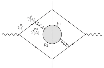
Figure 2: Double-real contributions that require special treatment in fdh to correct for unitarity violations. The blob represents either a quark, a gluon, or a ghost loop.

For our process such violations are restricted to the diagram shown in Figure 2. From a practical point of view, the problem can be understood by noting that evaluating the trace of the inner loop (either a quark, a gluon, or a ghost loop) gives rise to terms such as $p_{1}^{\alpha}\,p_{2}^{\beta}$, where $p_{1}$ and $p_{2}$ are the particle momenta and $\alpha$ and $\beta$ are the Lorentz indices of the inner loop. In order to evaluate these diagrams correctly, the angular average has to be performed in $d$ dimensions using identities like

$$p_{1}^{\alpha}\,p_{2}^{\beta} \to\frac{1}{4(d\!-\!1)}\Big{[}(d\!-\!2)\,(p_{12})^{\alpha}\,(p_{12})^{\beta}+(p_{12})^{2}\,g^{\alpha\beta}_{[d]}\Big{]}\,,$$ (32)

in agreement with (2.13) of Gnendiger:2017pys ; the external momentum is denoted by $p_{12}\!=\!p_{1}\!+\!p_{2}$. It is essential that on the right hand side the quasi $d$-dimensional metric is used. After the angular average, the resulting tensor can be contracted with the rest of the diagram and the remaining phase-space integrations can be performed. This procedure restores unitarity. While it is fairly simple for our process, it is rather tedious to implement for the general case.

In hv the situation is very similar. In fact, the relations between the partial results in hv and cdr are analogous to (30) and read

$$\sigma^{(vv)}_{{\rm\scriptscriptstyle HV}} =\frac{\sigma^{(vv)}_{{\rm\scriptscriptstyle CDR}}}{1-\epsilon}\,, \sigma^{(rr)}_{{\rm\scriptscriptstyle HV}} =\frac{\sigma^{(rr)}_{{\rm\scriptscriptstyle CDR}}}{1-\epsilon}\,, \sigma^{(rv)}_{{\rm\scriptscriptstyle HV}} =\frac{\sigma^{(rv)}_{{\rm\scriptscriptstyle CDR}}}{1-\epsilon}\,.$$ (33)

Again, combining the two-loop corrections and setting $d\!\to\!4$, we obtain the same physical cross section $\sigma^{(2)}$ in hv as in the other schemes. However, the double-real term is plagued by precisely the same unitarity-violating terms as in fdh and therefore requires the same unitarity-restoring treatment.

To summarize, fdh and hv can be used throughout for all parts of the computation. The combination of the intermediate results then leads to the same physical cross section. However, the treatment of the real corrections in fdh and hv is much more involved than in dred.

5 Conclusions

Extending previous studies to double-real and real-virtual corrections, we have investigated the regularization-scheme (in)dependence of a physical cross section at NNLO. As a case study we have considered two-jet production in electron-positron annihilation since for this process all computations can be done analytically.

One of the main findings is that in dred unitarity is preserved in the sense that the double-real and real-virtual corrections are obtained simply by integrating the corresponding four-dimensional real matrix element squared over the $d$-dimensional phase space. Terms of $\mathcal{O}(\epsilon/\epsilon)$ that have been missed with respect to cdr are precisely compensated by corresponding changes in the virtual contributions. As a consequence, the physical cross section is scheme independent, as required. This apparently magical conspiracy can be understood by systematically disentangling the ${d}_{s}$-dimensional vector fields of dred into ${d}$-dimensional gauge fields and $n_{\epsilon}$-dimensional $\epsilon$-scalar fields. Like for any other fields, cross sections involving $\epsilon$-scalars are finite and, as they come with a multiplicity of $n_{\epsilon}\!=\!2\epsilon$, they vanish in the limit $d\!\to\!4$.

Since the evanescent scalar fields do not contribute, an obvious way forward is to not compute their contributions in the first place. This corresponds to cdr. Alternatively, their contributions can be included. This corresponds to dred and, in fact, leads to simplifications in some aspects of the computation. While it can be debated at length which scheme is simpler to apply, the important main statement is that dred can be used systematically and without undue complications for arbitrary physical cross sections at NNLO. The practical steps required for the computation of the virtual, real, and real-virtual corrections are summarized as follows:

Guideline for the evaluation of NNLO virtual cross sections in DRED

• Split gauge fields in the initial and final state as well as gauge fields that connect 1PI subdiagrams similar to (12) into a quasi ${d}$-dimensional part and a quasi $n_{\epsilon}$-dimensional part. As a result, there are diagrams without $\epsilon$-scalars (type I) and diagrams where at least one gauge field is replaced by an $\epsilon$-scalar (type II).

• Evaluate type I contributions by using the (quasi) four-dimensional dred algebra. Since there are no $\epsilon$-scalars at the tree-level, evanescent couplings have to be considered only at one-loop and their renormalization has at most to be known at one-loop as well.

• Evaluate type II contributions by using the IR divergence formula (16). The finite part follows from the fact that the tree-level cross section is proportional to at least one power of $n_{\epsilon}\!=\!2\epsilon$. Similar to type I contributions, the renormalization of the evanescent couplings has at most to be known at one-loop order. In this way, no explicit two-loop computation with $\epsilon$-scalars has to be done.
  

Guideline for the evaluation of NNLO real cross sections in DRED

• Evaluate the real matrix element in ${d}_{s}\!=\!4$ dimensions which corresponds to setting $\epsilon\!\to\!0$ in the cdr result. The subsequent phase-space integration is done in the usual way in ${d}$ dimensions.

• If the phase-space integration is split into a finite and a singular part (through subtraction or slicing), the integrand in the finite part is evaluated in four dimension in any scheme. However, in dred even in the singular part the matrix element is only needed in four dimensions. As a result, in dred the $\mathcal{O}(\epsilon)$ terms of the (double) unresolved limits (e. g. triple-collinear or double-soft) are not required.

Guideline for the evaluation of NNLO real-virtual cross sections in DRED

• Evaluate the real-virtual contributions by using the (quasi) four-dimensional dred algebra. The subsequent loop and phase-space integrations are done in ${d}$ dimensions.

• Implement the UV renormalization by applying the split (12) at the tree-level and by taking into account the one-loop renormalization of the (evanescent) couplings.

Of course, it is also possible to use fdh or hv. The application of these schemes to two-loop amplitudes is well understood and transition rules between the various schemes are known. However, the naive use of fdh and hv for real corrections at NNLO leads to unitarity violations. In addition, the fdh and hv algebra gives rise to loop momenta that are not ${d}$-dimensional, but actually strictly four-dimensional. While it is possible to correct for these effects to obtain consistent results, it leads to additional complications.

With ever more complicated final states to be tackled at NNLO, it might well be worth to consider if computations in dred are not more efficient, even in non-supersymmetric theories. In particular, the presence of initial-state collinear singularities might further affect these considerations. Their consistent treatment at NNLO in dred remains to be worked out.

References

- (1) G. ’t Hooft and M. Veltman, Regularization and Renormalization of Gauge Fields, Nucl.Phys. B44 (1972) 189–213.
- (2) Z. Bern and D. A. Kosower, The Computation of loop amplitudes in gauge theories, Nucl.Phys. B379 (1992) 451–561.
- (3) W. Siegel, Supersymmetric Dimensional Regularization via Dimensional Reduction, Phys.Lett. B84 (1979) 193.
- (4) C. Gnendiger et al., To , or not to : recent developments and comparisons of regularization schemes, Eur. Phys. J. C77 (2017) 471, [1705.01827].
- (5) Z. Kunszt, A. Signer and Z. Trocsanyi, One loop helicity amplitudes for all 2 2 processes in QCD and N=1 supersymmetric Yang-Mills theory, Nucl.Phys. B411 (1994) 397–442, [hep-ph/9305239].
- (6) S. Catani, S. Dittmaier and Z. Trocsanyi, One loop singular behavior of QCD and SUSY QCD amplitudes with massive partons, Phys. Lett. B500 (2001) 149–160, [hep-ph/0011222].
- (7) S. Catani, M. H. Seymour and Z. Trocsanyi, Regularization scheme independence and unitarity in QCD cross-sections, Phys. Rev. D55 (1997) 6819–6829, [hep-ph/9610553].
- (8) A. Signer and D. Stöckinger, Factorization and regularization by dimensional reduction, Phys.Lett. B626 (2005) 127–138, [hep-ph/0508203].
- (9) A. Signer and D. Stöckinger, Using Dimensional Reduction for Hadronic Collisions, Nucl.Phys. B808 (2009) 88–120, [0807.4424].
- (10) D. Capper, D. Jones and P. van Nieuwenhuizen, Regularization by Dimensional Reduction of Supersymmetric and Nonsupersymmetric Gauge Theories, Nucl.Phys. B167 (1980) 479.
- (11) I. Jack, D. Jones and K. Roberts, Dimensional reduction in nonsupersymmetric theories, Z.Phys. C62 (1994) 161–166, [hep-ph/9310301].
- (12) I. Jack, D. Jones and K. Roberts, Equivalence of dimensional reduction and dimensional regularization, Z.Phys. C63 (1994) 151–160, [hep-ph/9401349].
- (13) R. Harlander, P. Kant, L. Mihaila and M. Steinhauser, Dimensional Reduction applied to QCD at three loops, JHEP 0609 (2006) 053, [hep-ph/0607240].
- (14) R. Harlander, D. Jones, P. Kant, L. Mihaila and M. Steinhauser, Four-loop beta function and mass anomalous dimension in dimensional reduction, JHEP 0612 (2006) 024, [hep-ph/0610206].
- (15) W. B. Kilgore, Regularization Schemes and Higher Order Corrections, Phys.Rev. D83 (2011) 114005, [1102.5353].
- (16) W. B. Kilgore, The Four Dimensional Helicity Scheme Beyond One Loop, Phys.Rev. D86 (2012) 014019, [1205.4015].
- (17) C. Gnendiger, A. Signer and D. Stöckinger, The infrared structure of QCD amplitudes and in FDH and DRED, Phys.Lett. B733 (2014) 296–304, [1404.2171].
- (18) A. Broggio, C. Gnendiger, A. Signer, D. Stöckinger and A. Visconti, Computation of in and : renormalization, operator mixing, and explicit two-loop results, Eur. Phys. J. C75 (2015) 418, [1503.09103].
- (19) A. Broggio, C. Gnendiger, A. Signer, D. Stöckinger and A. Visconti, SCET approach to regularization-scheme dependence of QCD amplitudes, JHEP 01 (2016) 078, [1506.05301].
- (20) C. Gnendiger, A. Signer and A. Visconti, Regularization-scheme dependence of QCD amplitudes in the massive case, JHEP 10 (2016) 034, [1607.08241].
- (21) M. Czakon and D. Heymes, Four-dimensional formulation of the sector-improved residue subtraction scheme, Nucl. Phys. B890 (2014) 152–227, [1408.2500].
- (22) C. Anastasiou, K. Melnikov and F. Petriello, Real radiation at NNLO: jets through O(alpha**2(s)), Phys. Rev. Lett. 93 (2004) 032002, [hep-ph/0402280].
- (23) A. Gehrmann-De Ridder, T. Gehrmann and E. W. N. Glover, Infrared structure of jets at NNLO, Nucl. Phys. B691 (2004) 195–222, [hep-ph/0403057].
- (24) B. Page and R. Pittau, NNLO final-state quark-pair corrections in four dimensions, Eur. Phys. J. C79 (2019) 361, [1810.00234].
- (25) R. Pittau, A four-dimensional approach to quantum field theories, JHEP 11 (2012) 151, [1208.5457].
- (26) A. M. Donati and R. Pittau, FDR, an easier way to NNLO calculations: a two-loop case study, Eur. Phys. J. C74 (2014) 2864, [1311.3551].
- (27) M. D. Sampaio, A. P. Baeta Scarpelli, J. E. Ottoni and M. C. Nemes, Implicit regularization and renormalization of QCD, Int. J. Theor. Phys. 45 (2006) 436–457, [hep-th/0509102].
- (28) H. G. Fargnoli, A. P. Baeta Scarpelli, L. C. T. Brito, B. Hiller, M. Sampaio, M. C. Nemes et al., Ultraviolet and Infrared Divergences in Implicit Regularization: A Consistent Approach, Mod. Phys. Lett. A26 (2011) 289–302, [1001.1543].
- (29) A. L. Cherchiglia, M. Sampaio and M. C. Nemes, Systematic Implementation of Implicit Regularization for Multi-Loop Feynman Diagrams, Int. J. Mod. Phys. A26 (2011) 2591–2635, [1008.1377].
- (30) Y.-L. Wu, Symmetry preserving loop regularization and renormalization of QFTs, Mod. Phys. Lett. A19 (2004) 2191–2204, [hep-th/0311082].
- (31) D. Bai and Y.-L. Wu, Quadratic Contributions of Softly Broken Supersymmetry in the Light of Loop Regularization, Eur. Phys. J. C77 (2017) 617, [1706.06798].
- (32) R. J. Hernandez-Pinto, G. F. R. Sborlini and G. Rodrigo, Towards gauge theories in four dimensions, JHEP 02 (2016) 044, [1506.04617].
- (33) F. Driencourt-Mangin, G. Rodrigo, G. F. R. Sborlini and W. J. Torres Bobadilla, Universal four-dimensional representation of at two loops through the Loop-Tree Duality, JHEP 02 (2019) 143, [1901.09853].
- (34) D. Stckinger, Regularization by dimensional reduction: consistency, quantum action principle, and supersymmetry, JHEP 0503 (2005) 076, [hep-ph/0503129].
- (35) W. Celmaster and R. J. Gonsalves, An Analytic Calculation of Higher Order Quantum Chromodynamic Corrections in e+ e- Annihilation, Phys. Rev. Lett. 44 (1980) 560.
- (36) K. G. Chetyrkin, A. L. Kataev and F. V. Tkachov, Higher Order Corrections to Sigma-t (e+ e- Hadrons) in Quantum Chromodynamics, Phys. Lett. 85B (1979) 277–279.
- (37) G. Kramer and B. Lampe, Two Jet Cross-Section in e+ e- Annihilation, Z. Phys. C34 (1987) 497.
- (38) T. Matsuura and W. L. van Neerven, Second Order Logarithmic Corrections to the Drell-Yan Cross-section, Z. Phys. C38 (1988) 623.
- (39) T. Matsuura, S. C. van der Marck and W. L. van Neerven, The Calculation of the Second Order Soft and Virtual Contributions to the Drell-Yan Cross-Section, Nucl. Phys. B319 (1989) 570–622.
- (40) S. Catani, The Singular behavior of QCD amplitudes at two loop order, Phys.Lett. B427 (1998) 161–171, [hep-ph/9802439].
- (41) T. Becher and M. Neubert, Infrared singularities of scattering amplitudes in perturbative QCD, Phys.Rev.Lett. 102 (2009) 162001, [0901.0722].
- (42) E. Gardi and L. Magnea, Factorization constraints for soft anomalous dimensions in QCD scattering amplitudes, JHEP 03 (2009) 079, [0901.1091].
- (43) T. Becher and M. Neubert, On the Structure of Infrared Singularities of Gauge-Theory Amplitudes, JHEP 0906 (2009) 081, [0903.1126].
- (44) E. Gardi and L. Magnea, Infrared singularities in QCD amplitudes, Nuovo Cim. C32N5-6 (2009) 137–157, [0908.3273].
- (45) M.-x. Luo, H.-w. Wang and Y. Xiao, Two loop renormalization group equations in general gauge field theories, Phys.Rev. D67 (2003) 065019, [hep-ph/0211440].
- (46) A. Gehrmann-De Ridder, T. Gehrmann and G. Heinrich, Four particle phase space integrals in massless QCD, Nucl. Phys. B682 (2004) 265–288, [hep-ph/0311276].
- (47) A. Smirnov, Algorithm FIRE – Feynman Integral REduction, JHEP 0810 (2008) 107, [0807.3243].
- (48) R. A. Fazio, P. Mastrolia, E. Mirabella and W. J. Torres Bobadilla, On the Four-Dimensional Formulation of Dimensionally Regulated Amplitudes, Eur. Phys. J. C74 (2014) 3197, [1404.4783].
- (49) C. Gnendiger and A. Signer, in the four-dimensional helicity scheme, Phys. Rev. D97 (2018) 096006, [1710.09231].