Attributed Relational SIFT-based Regions Graph (ARSRG): concepts and applications

Abstract

Graphs are widely adopted tools for encoding information. Generally, they are applied to disparate research fields where data needs to be represented in terms of local and spatial connections. In this context, a structure for ditigal image representation, called Attributed Relational SIFT-based Regions Graph (ARSRG), previously introduced (?, ?, ?, ?), is presented. ARSRG has not been explored in detail in previous works and for this reason the goal is to investigate unknown aspects. The study is divided into two parts. A first, theoretical, introducing formal definitions, not yet specified previously, with purpose to clarify its structural configuration. A second, experimental, which provides fundamental elements about its adaptability and flexibility regarding different applications. The theoretical vision combined with the experimental one shows how the structure is adaptable to image representation including contents of different nature.

1 Introduction

Among issues related human vision the processing of visual complex entities is one of most important. The processing of information is often based on local-to-global or global-to-local connections (?). Local-to-global concept concerns the transitions from local details of scene to global configuration, while global-to-local works in the reverse order, from global configuration towards the details. For example an algorithm for face recognition, which use local-to-global approach, starts eyes, nose and ears recognition, and finally brings to face configuration. Differently, a global-to-local algorithm first identifies the face that leads to the identification of details (eyes, nose and ears). During the task of human recognition global configuration of a scene plays a key role, especially when subjects see the images for a short duration of time. Also, humans leverage local information in effect way to recognize scene categories. Theories of higher-level visual perception split individual elements at the local level and global objects, for which the information on many local components are perceptually grouped (?). Graphs are frequently adopted to represent information in terms of nodes and edges, where relations among data must be highlighted and generally occur in raw form. Computer Vision, Pattern Recognition and many other fields benefit from data graph representations and related manipulation algorithms. Specifically, in the Image Processing field, graphs are used to represent digital images in many ways. Standard approach concerns partitioning of the image into dominant disjoint regions, where local and spatial features are respectively nodes and edges. Local features describe intrinsic properties of regions (such as shape, colors, texture), while spatial features provide topological information about neighborhood. Image representation is one of the crucial steps for systems working in the Image Retrieval field. Modern Content Based Image Retrieval (CBIR) systems consider essentially the image basic elements (colors, textures, shapes and topological relationships) extracted from the entire image, in order to provide an effective representation. Through the analysis of these elements, compositional structures are produced. Other systems, called Region Based Image Retrieval (?) (RBIR), focus their attention on specific image regions instead of the entire content to extract features. In this paper, a graph structure for image representation, called Attributed Relational SIFT-based Regions Graph (ARSRG), is described, analyzed and discussed with reference to previous works (?, ?, ?, ?). In particular, new definitions and properties arising from the detailed analysis of the structure are introduced. Finally, through a wide experimental phase, how the structure is adaptable to different types of application contexts is shown. The paper is organized as follows: section 2 includes related research about graph based image representation including Scale Invariant Feature Transform (SIFT) (?). Sections 3, 4, 5 are dedicated to ARSRG description, definitions and properties. Experimental results and conclusions are respectively reported in section 6 and section 7.

2 Related work

The literature reports many approaches which combine local and spatial information arising from SIFT features. Commonly, a graph structure encodes information about keypoints located in a certain position of image. Nodes represent SIFT descriptors, while edges describe spatial relationships between different keypoints.

In (?) a graph $G_{1}$ represents a set of SIFT keypoints from the image $I_{1}$ and is defined as

$$G_{1}=(V_{1},M_{1},Y_{1})$$ (1)

where $v_{\alpha}\in V_{1}$ is a node associated to a SIFT keypoint with position $(p_{1}^{(\alpha)},p_{2}^{(\alpha)})$, $y_{\alpha}\in Y_{1}$ is the SIFT descriptor attached to node $v_{\alpha}$ and $M_{1}$ is the adjacency matrix. If $M_{1\;\alpha\beta}=1$ the nodes $v_{\alpha}$ and $v_{\beta}$ are adjacent, $M_{1\;\alpha\beta}=0$ otherwise.

In (?) authors combine local information of SIFT features with global geometrical information in order to estimate a robust set of features-matches. These information are encoded using a graph structure

$$G_{0}=(V_{0},B,Y)$$ (2)

where $v\in V_{0}$ is a node associated to a SIFT keypoint, $B$ is the adjacency matrix, $B_{v,v^{\prime}}=1$ if the nodes $v$ and $v^{\prime}$ are connected $B_{v,v^{\prime}}=0$ otherwise, while $y_{v}\in Y$ is the SIFT descriptor associated to node $v$.

In (?) nodes are associated to $N$ image regions related to an image grid, while edges connect each node with its four neighbors. Basic elements are not pixels but regions extended in the $x$ (horizontal) and $y$ (vertical) directions. The nodes are identified using their coordinates on the grid. The spatial information associated to nodes are indices $d_{n}=(x_{n},y_{n})$. Also, a feature vector $F_{n}$ is associated with the corresponding image region and, then, to node. The image is divided into overlapping regions of $32$ $\times$ $32$ pixels. Four $128$-dimensional SIFT descriptors, for each region, are extracted and concatenated.

In (?) the graph based image representation includes SIFT features, MSER (?) and Harris-Affine (?). Given two graphs $G^{P}=(V^{P},E^{P},A^{P})$ and $G^{P}=(V^{Q},E^{Q},A^{Q})$, representing images $I^{P}$ and $I^{Q}$, $V$ is the set of nodes, image features extracted, $E$ the set of edges, features spatial relations, and $A$ the set of attributes, information associated to features extracted.

In (?) SIFT features are combined in form of hyper-graph. A hyper-graph $G=(V,E,A)$ is composed of nodes $v\in V$, hyper-edges $e\in E$, and attributes $a\in A$ associated with the hyper-edges. A hyper-edge $e$ encloses a subset of nodes with size $\delta(e)$ from $V$, where $\delta(e)$ represents the order of an hyper-edge.

In (?) an approach to $3$D objects recognition is presented. Graph matching framework is used in order to enable the utilization of SIFT features and to improve robustness. Differently to standard methods, test images are not converted into finite graphs through operations of discretization or quantization. Then, continuous graph space is explored in the test image at detection time. To this end, local kernels are applied to indexing image features and to enable a fast detection.

In (?) an approach to matching features problem with application of scene recognition and topological SLAM is proposed. For this purpose, the scene images are encoded using a particular data structure. Image representation is built through two steps: image segmentation using JSEG (?) algorithm and invariant feature extraction MSER and SIFT descriptors in a combined way.

In (?) SIFT features based on visual saliency and selected to construct object models are extracted. A Class Specific Hypergraph ($CSHG$) to model objects in compact way is introduced. The hypergraphs are built on different Delaunay graphs. Each one is created from a set of selected SIFT features using a single prototype image of an object. Using this approach, the object models can be represented through a minimum of object views.

In (?) a method for generic object recognition through graph structural expression using SIFT features is described. A graph structure is created using lines to connect SIFT keypoints. The graph is represented as $G=(V,E,X)$ where $E$ represents the set of edges, $V$ is the set of vertices and $X$ the set of their associated labels, SIFT descriptors. The node represents a keypoint detected by SIFT algorithm and the associated label is the $128$-dimension SIFT descriptor. The edge $e_{\alpha\beta}\in E$ connects two nodes $u_{\alpha}\in V$ and $u_{\beta}\in V$. The graph is complete when all keypoints extracted from the image are connected by edges. Formally, the set of edges is defined as follows:

$$E=\left\{e_{ij}\mid\forall i,j\frac{\parallel p_{i}-p_{j}\parallel}{\sqrt{\sigma_{i}\sigma_{j}}}<\lambda\right\}$$ (3)

where $p=(p_{x},p_{y})$ represents keypoint spatial coordinates, $\sigma$ its scale, and $\lambda$ is a threshold value. An edge does not exist when the value is greater than the threshold $\lambda$. In this way, an extra edge is not created. This formulation of proximity graph reduces the computation complexity and, at same time, improves the detection performance.

In (?) a median K-nearest-neighbor (K-NN) graph $G_{P}=(V_{P},E_{P})$ is built. A vertex $v_{i}$ for each of the $N$ points $p_{i}$ is created, with $V_{P}=v_{1},...,v_{N}$. Also, a non-directed edge $(i,j)$ is created when $p_{j}$ is one of the $K$ closest neighbors of $p_{i}$ and $\parallel p_{i}-p_{j}\parallel\leq\eta$. $\eta$ is the median of all distances between pairs of vertices and is defined as:

$$\eta=median_{(l,m)\in V_{P}\times V_{P}}||p_{l}-p_{m}||$$ (4)

If there are not $K$ vertices that support the structure of $p_{i}$ then this vertex is completely disconnected until the end of the K-NN graph construction. The graph $G_{P}$ has the $N\times N$ adjacency matrix $A_{P}$, where $A_{P}(i,j)=1$ when $(i,j)\in E_{P}$ and $A_{P}(i,j)=0$ otherwise.

3 Attributed Relational SIFT-based Regions Graph (ARSRG)

In this section Attributed Relational SIFT-based Regions Graph (ARSRG) is introduced based on two main steps: features extraction and graph construction. The first step consists of Regions of Interest (ROIs) extraction from the image through a segmentation technique. Connected components in the image are then identified with the aim of building the Region Adjacency Graph (RAG) (?), to encode spatial relations between image regions. Simultaneously, SIFT (?) descriptors are extracted from the original image, in order to ensure invariance to image rotation, scaling, translation, illumination changes and projective transforms. The second step consists in the construction of graph structure. ARSRG is composed of three levels: root node, RAG nodes and leaf nodes. At first level, the root node represents the image and is linked to all RAG nodes at the second level. RAG nodes encode adjacency relationships between different image regions. Thus, adjacent regions in the image are represented by connected nodes. In addition, each RAG node is connected with the Root node at the higher level. Finally, the leaf nodes represent the set of SIFT descriptors extracted from the image. At third level, two types of configurations are provided: Region based and Region graph based. In the Region based configuration, a keypoint is associated to a region based on its spatial coordinates, whereas Region graph based configuration describes keypoints belonging to the same region connected by edges (which encode spatial adjacency). Below, the steps of features extraction and graph construction are described in detail.

3.1 Features extraction

3.1.1 Region of interests (ROIs) extraction

ROIs from the image through a segmentation algorithm called JSEG (?) are extracted. JSEG performs segmentation through two different steps: color quantization and spatial segmentation. First step consists in a coarse quantization without degrading the image quality significantly. In the second step, a spatial segmentation directly on the class-map without taking into account the color similarity of the corresponding pixel is performed.

3.1.2 Labeling connected components

The next step involves the labeling of connected components on the segmentation result. A connected component is an image region consisting of contiguous pixels of the same color. The process of connected components labeling of an image $B$ produces an output image $LB$ that contain labels (positive integers or characters). A label is a symbol naming an entity exclusively. Regions connected by the $4$-neighborhood and $8$-neighborhood will have the same label. Algorithm 1 shows a version of connected components labeling.

Algorithm 1 $Connected\;Components\;Labeling$

0:  $I$ - Image to Label;

0:  $I$ - Image Labeled;

1:  m=0

2:  for y=1:$I\_size\_y$ do

3:     for x=1:$I\_size\_x$ do

4:        if I[i][j] == 0 then

5:           m=m+1

6:           $Component\;Label(I,x,y,m)$

7:        end if

8:     end for

9:  end for

10:  return  I

Algorithm 2 $Component\;Label$

0:  $I$ - Image to Label; $i,j$ - image index; $l$ - label;

0:  $\oslash$;

1:  if I[i][j] == 0 then

2:     I[i][j]=m

3:     $Component\;Label(I,i-1,j-1,m)$

4:     $Component\;Label(I,i-1,j,m)$

5:     $Component\;Label(I,i-1,j+1,m)$

6:     $Component\;Label(I,i,j-1,m)$

7:     $Component\;Label(I,i,j+1,m)$

8:     $Component\;Label(I,i+1,j-1,m)$

9:     $Component\;Label(I,i+1,j,m)$

10:     $Component\;Label(I,i+1,j+1,m)$

11:  end if

3.1.3 Region Adjacency Graph (RAG) structure

The Region Adjacency Graph (RAG) (?) is adopted to build a graph based image representation located at second level of the ARSRG structure. Based on image segmentation result, a region represents an elementary component of the image. RAG is built with reference to spatial relations between regions. Two regions are defined to be adjacent if they share the same boundary. In the RAG, a node represents a region, and an edge represents adjacency between two nodes. The RAG is defined as a graph $G=(V,E)$, where nodes are regions in $V$ and edges $E$ identify the boundaries that connect them. Moreover, the RAG connectivity is invariant to translations and rotations, which is a useful property for a high-level image representation. In the algorithm 3, a pseudocode version of RAG algorithm is shown.

Algorithm 3 $Region\;Adjacency\;Graph$

0:  $Labeled\_image$;

0:  $Graph$ $Structure$ $(Adjacency\_matrix)$;

1:  $Adjacency\_matrix=0$

2:  for $pixel(i,j)\in Labeled\_image$ do

3:     for $pixel(x,y)\in 8-neighborhood$ do

4:        if $pixel(i,j)\neq pixel(x,y)$ then

5:           $Adjacency\_matrix(pixel(i,j),pixel(x,y))=1$

6:        end if

7:     end for

8:  end for

9:  return  $Adjacency\_matrix$

3.1.4 Scale Invariant Feature Transform (SIFT)

SIFT (?) descriptors are extracted to ensure invariance to rotation, scaling, translation, partial illumination changes and projective transform in the image description. SIFT are computed during the features extraction phase, through a parallel task respect to RAG creation.

3.2 Graph construction

ARSRG building process consists in creation of three levels :

1. Root node. The node located at the first level of graph structure and represents the image. It is connected to all nodes at next level.

2. Region Adjacency Graph (RAG) nodes. Adjacency relations among different image regions based on the segmentation result. Thus, adjacent image regions are represented by nodes connected at this level.

3. Leaf nodes. The set of SIFT features extracted from the image. Two type of connections are provided:

   1. Region based. A leaf node represents a SIFT keypoint obtained during features extraction. Each leaf node-keypoint is associated to a region based on its spatial coordinates in the image. At this level, each node is connected with just one RAG higher level node (fig. 1(a)).

   2. Region graph based. In addition to the previous configuration, leaf nodes-keypoints belonging to the same region are connected by edges, which encode spatial adjacency, based on a thresholding criteria (fig. 1(b)).

(a)

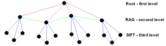
(b)

Figure 1: Region based (a) and Region graph based (b) configurations.

4 Formal definitions

ARSRG structure is defined based on two leaf node configurations.

Definition 4.1

ARSRG${}_{1^{st}}$ (first leaf nodes configuration) $G$ is defined as a tuple $G=(V_{regions},E_{regions},VF_{SIFT},E_{regions-SIFT})$, where

• $V_{regions}$, the set of regions-nodes.

• $E_{regions}\subseteq V_{regions}\times V_{regions}$, the set of undirected edges, where $e\in E_{regions}$ and $e=(v_{i},v_{j})$ is an edge that connect nodes $v_{i},v_{j}\in V_{regions}$.

• $VF_{SIFT}$, the set of SIFT-nodes.

• $E_{regions-SIFT}\subseteq V_{regions}\times VF_{SIFT}$, the set of directed edges, where $e\in E_{regions-SIFT}$ and $e=(v_{i},vf_{j})$ is an edge that connect source node $v_{i}\in V_{regions}$ and destination node $vf_{j}\in VF_{SIFT}$.

Definition 4.2

ARSRG${}_{2^{nd}}$ (second leaf nodes configuration), $G$ is defined as a tuple $G=(V_{regions},E_{regions},VF_{SIFT},E_{regions-SIFT},E_{SIFT})$, where:

• $V_{regions}$, the set of regions-nodes.

• $E_{regions}\subseteq V_{regions}\times V_{regions}$, the set of undirected edges, where $e\in E_{regions}$ and $e=(v_{i},v_{j})$ is an edge that connect nodes $v_{i},v_{j}\in V_{regions}$

• $VF_{SIFT}$, the set of SIFT-nodes.

• $E_{regions-SIFT}\subseteq V_{regions}\times VF_{SIFT}$, the set of directed edges, where $e\in E_{regions-SIFT}$ and $e=(v_{i},vf_{j})$ is an edge that connect source node $v_{i}\in V_{regions}$ and destination node $vf_{j}\in VF_{SIFT}$.

• $E_{SIFT}\subseteq VF_{SIFT}\times VF_{SIFT}$, the set of undirected edges, where $e\in E_{SIFT}$ and $e=(vf_{i},vf_{j})$ is an edge that connect nodes $vf_{i},vf_{j}\in V_{SIFT}$

ARSRG structures, first and second leaf node configuration, are created based on definitions 4.1 and 4.2. The nodes belonging to sets $V_{regions}$ and $VF_{SIFT}$ are associated to features extracted from the image. Particularly:

Definition 4.3

$F_{regions}$ is a set of vectors attributes associated to nodes in $V_{regions}$. An element, $f_{i}\in v_{i}$, is associated to a node of ARSRG structure at second level. It contains the region dimension (pixels).

Definition 4.4

$F_{SIFT}$ is a set of vectors attributes associated to nodes in $VF_{SIFT}$. An element, $f_{i}\in vf_{i}$, is associated to a node of ARSRG structure at third level. It contains a SIFT descriptor.

The association between features and nodes is performed through assignment functions defined as follows:

Definition 4.5

The node-labeling function $L_{regions}$ assigns a label to each node $v\in V_{regions}$ of ARSRG at the second level. The node label is a feature attribute $d_{i}$ extracted from the image. The label value is the dimension of region (pixels number). The labeling procedure of a $v$ node occurs during the process of ARSRG construction.

Definition 4.6

The SIFT node-labeling function $L_{SIFT}$ assigns a label to each node $vf\in VF_{SIFT}$ of ARSRG at third level. The node label is a features vector $f_{i}$, keypoint, extracted from the image. The labeling procedure of a $vf$ node checks the position of keypoint in the image compared to the region to which it belongs.

Also, the RAG nodes $\in V_{regions}$ are doubly linked in horizontal order, between them, and vertical order, with nodes $\in VF_{SIFT}$. Edges $\in E_{regions}$ are all undirected from left to right. While, edges $\in E_{regions-SIFT}$ are all directed from top to bottom. The Root node maintains list of edges outgoing to RAG nodes. Also, each RAG node maintains three linked lists of edges: one for outgoing to RAG nodes, one for outgoing leaf nodes and one for ingoing to Root node. Finally, each leaf node maintains two linked lists of edges: one for ingoing from RAG nodes and one for outgoing leaf nodes. The edges in each list are ordered based on distances between end nodes: shorter edges come first. These lists of edges have direct geometrical meanings: each node is connected to another node in one direction: left, right, top, and bottom.

A very important aspect concerns the organization of the third level of the ARSRG structure. To this end, SIFT Nearest-Neighbor Graph ($SNNG$) is introduced.

Definition 4.7

A $SNNG=(VF_{SIFT},E_{SIFT})$ is defined as

• $VF_{SIFT}$: the set of nodes associated to SIFT keypoints

• $E_{SIFT}$: the set of edges, where for each $v_{i}\in VF_{SIFT}$, an edge $(v_{i},v_{ip})$ if and only if $dist(v_{i},v_{ip})<\tau$ exists. $dist(v_{i},v_{ip})$ is Euclidean distance applied to $x$ and $y$ position of keypoints in the image, $\tau$ is a threshold value and $p$ stems from $1$ to $k$, $k$ being the size of $VF_{SIFT}$.

This notation is very useful during the matching phase. Indeed, each $SNNG$ indicates the set of SIFT features belonging to image region, with reference to definition 4.2, and represents SIFT features organized from local and spatial point of view. A different version of $SNNG$ is called complete SIFT Nearest-Neighbor Graph ($SNNGc$).

Definition 4.8

A $SNNGc=(VF_{SIFT},E_{SIFT})$ is defined as

• $VF_{SIFT}$: the set of nodes associated to SIFT keypoints

• $E_{SIFT}$: the set of edges, where for each $v_{i}\in VF_{SIFT}$, an edge $(v_{i},v_{ip})$ if and only if $dist(v_{i},v_{ip})<\tau$ exists. $dist(v_{i},v_{ip})$ is Euclidean distance applied to $x$ and $y$ position of keypoints in the image, $\tau$ is a threshold value and $p$ stems from $1$ to $k$, $k$ being the size of $VF_{SIFT}$. In this case, $\tau$ is greater than the maximal distance between keypoints.

Another important aspect concerns the difference between vertical and horizontal relationships among nodes in the ARSRG structure. Below these relations, edges, are defined.

Definition 4.9

A region horizontal edge $e$, $e\in E_{regions}$, is an undirected edge $e=(v_{i},v_{j})$ that connects nodes $v_{i},v_{j}\in V_{regions}$.

Definition 4.10

A SIFT horizontal edge $e$, $e\in E_{SIFT}$, is an undirected edge $e=(vf_{i},vf_{j})$ that connects nodes $vf_{i},vf_{j}\in V_{SIFT}$.

Definition 4.11

A vertical edge $e$, $e\in E_{regions-SIFT}$, is an directed edge $e=(v_{i},vf_{j})$ that connects nodes $v_{i}\in V_{regions}$ and $vf_{j}\in VF_{SIFT}$ from source node $v_{i}$ to destination node $vf_{j}$.

As can be noted horizontal edges connect nodes of the same level. While, vertical edges connect nodes of different levels (second-third). Finally, these relations are represented through adjacency matrices defined below.

Definition 4.12

The binary regions adjacency matrix $S_{regions}$ describes the spatial relations among RAG nodes. An element $s_{ij}$ defines an edge, $e=(v_{i},v_{j})$, connecting nodes $v_{i},v_{j}\in V_{regions}$. Hence, an element $s_{ij}\in S_{regions}$ is set to $1$ if node $v_{i}$ is connected to node $v_{j}$, $0$ otherwise.

Definition 4.13

The binary SIFT adjacency matrix $S_{SIFT}$ describes the spatial relations among leaf nodes. An element $s_{ij}$ defines an edge, $e=(vf_{i},vf_{j})$, connecting nodes $vf_{i},vf_{j}\in VF_{SIFT}$. Hence, an element $s_{ij}\in S_{SIFT}$ is set to $1$ if node $vf_{i}$ is connected to node $vf_{j}$, $0$ otherwise.

Figures 2 show the two different ARSRG structures on a sample image.

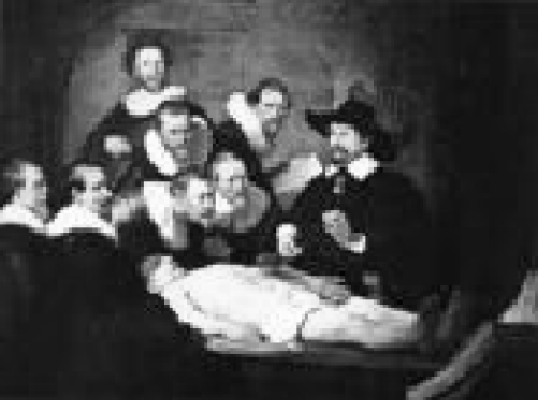
(a)

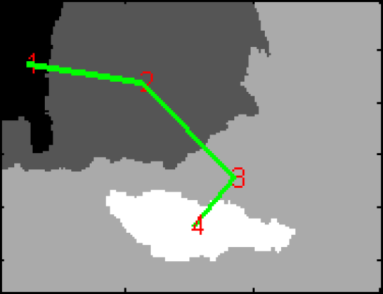
(b)

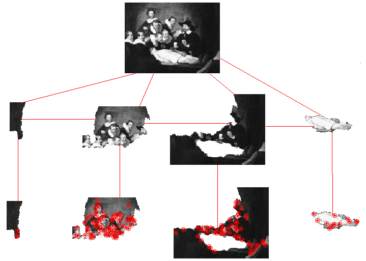
(c)

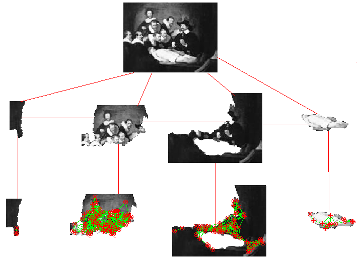
(d)

Figure 2: (a) Original image; (b) RAG composed of $4$ regions; (c) Region based leaf node configuration; (d) Region graph based leaf node configuration. Red point in figures (c) and (d) represent SIFT keypoints belonging to regions. While green lines in the figure (d) represent the edges of graph based leaf node configuration.

5 Properties

In this section, ARSRG structure properties arising from features extraction and graph construction steps are highlighted.

Region features and structural information. The main goal of the ARSRG structure is to connect regional features and structural information. First step concerns image segmentation in order to extract ROIs. This is a step towards the extraction of semantic information from a scene. Once the image has been segmented, the RAG structure is created. This features representation highlights individual regions and spatial relations existing between them.

Horizontal and vertical relations. ARSRG structure presents two types of relations (edges) between image features: horizontal and vertical. Vertical edges define image topological structure, while horizontal edges define spatial constraints about nodes (regions) features. Horizontal relations (definitions 4.9 and 4.10) concern ROIs and SIFT features located at the second level of the structure. The general goal is to provide information of spatial closeness, define spatial constraints on the node attributes, characterize features map of specific resolution level (detail) on a defined image and can be differentiated according to the computational complexity and the occurrence frequency. Their order is in the range $\{1,\dots,n\}$, where $n$ is the number of features specified through the relations. In a different way, vertical relations (definition 4.11) concern connections between individual regions and their features. The vertical directed edges connect nodes among second and third levels of ARSRG (RAG nodes to leaf nodes) and provide a parent-child relationship. In this context, the role of ARSRG structure is to create a bridge between the defined relations. This aspect leads to some advantages, i.e. the possibility to explore the structure both to in breadth and depth during the matching process.

Region features invariant to point of view, illumination and scale. Building local invariant region descriptors is a hot topic of research with a set of applications such as object recognition, matching and reconstruction. Over the last years, great success has been achieved in designing descriptors invariant to certain types of geometric and photometric transformations. Local Invariant Features Extraction (LIFE) methods work in order to extract stable descriptors starting from a particular set of characteristic regions of the image. LIFE methods were chosen, for region representation, in order to provide invariance to certain conditions. These local representations, created by using information extracted from each region, are robust to certain image deformations such as illumination and viewpoint changing. ARSRG structure includes SIFT features, identified in (?) as the most stable representations between different LIFE methods.

Advantages due to detailed information located on different level. The detailed image description, provided by the ARSRG structure, represents an advantage during the comparison phase. In hierarchical way, the matching procedure explores global, local and structural information, within ARSRG. First step involves a filtering procedure for regions based on size. Small regions, containing poor information, are removed. Subsequently, the matching procedure goes to next level of the ARSRG structure analyzing features of single regions to obtain a stronger match. The goal is to solve the mapping on multiple SNNGs (definition 4.7) of the ARSRGs. In essence, this criterion identifies partial matches among SNNGs belonging to ARSRGs. During the procedure, different combinations of graph SNNGs are identified and a hierarchy of the matching process is constructed. In this way, the overall complexity is reduced, which is expected to show considerable advantage especially for large ARSRGs.

Advantages due to match region-by-region. Region-Based Image Retrieval (RBIR) (?) systems work with the goal of extracting and defining similarity between two images based on regional features. It has been demonstrated that users focus their attention on specific regions rather than the entire image. Region based image representation has proven to be more close to human perception. In this context, in order to compare ARSRG structures, a region matching scheme based on appearance similarities of image segmentation results can be adopted. Region matching algorithm exploits the regions provided by segmentation and compares the features associated to them. The pairwise region similarities are computed from a set of SIFT features belonging to regions. The matching procedure is asymmetric. The input image is segmented into regions and its groups of SIFT keypoints can be matched within consistent portion of the other image. In this way, segmentation result is used to create regions of candidate keypoints, avoiding incompatible regions for two images of the same scene.

False matches removal. One of the main issues of LIFE methods concerns the removal of false matches. It has been shown that LIFE methods produce a number of false matches, during the comparison phase, that significantly affect accuracy. The main reason concerns the lack of correspondence among image features (for example due to partial background occlusion of the scene). Standard similarity measures, based on the features descriptor, are widely used, even if they rely only on region appearance. In some cases, it cannot be sufficiently discriminating to ensure correct matches. This problem is more relevant in the presence of low or homogeneous textures, and leads to a lot of false matches. The application of the ARSRG structure provides a solution for this problem. In order to reduce false matches, small ARSRG regions-nodes, and associated SIFT descriptors, are removed. Indeed, small regions and their associated features are not very informative both in image description and matching. Ratio test (?) or graph matching (?) can be applied to perform comparison between remaining regions. This filtering procedure has a strong impact on experiments, resulting in a relevant accuracy improvement.

6 Experimental results

This section provides experimental results arising from different application fields. Particularly:

1. Graph matching (?). ARSRG is adopted to address the art painting retrieval problem. A graph matching algorithm is adopted to measure ARSRGs similarities exploiting local information and topological relations.

2. Graph embedding (?). ARSRG is adopted to effectively tackle the object recognition problem. A framework to embed graph structures into vector space is built;

3. Bag of Graph Words (?). ARSRG is adopted to address the image classification problem. A digital image is described as a vector in terms of a frequency histogram of ARSRGs.

4. Kernel Graph Embedding (?). ARSRG is adopted to effectively tackle the imbalanced classification problem. A digital image is described through a vector-based representation called Kernel Graph Embedding on Attributed Relational Scale-Invariant Feature Transform-based Regions Graph (KGEARSRG).

6.1 Graph matching

In this section the results related to the work proposed in (?) are analyzed. ARSRG has been tested on three datasets and compared with LIFE methods, graph matching algorithms and a CBIR system. The first dataset, described in (?), is composed by two sets of images obtained from Olga’s gallery and Travel Webshots. The second dataset, described in(?), is composed by painting photos taken from the Cantor Arts Center. The third dataset, described in (?), is composed by $1002$ images. Figure 3 shows some examples.

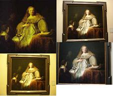
(a)

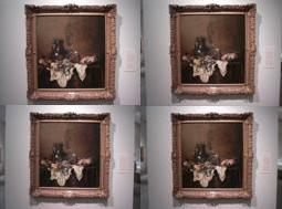
(b)

Figure 3: Some examples of art painting images.

6.1.1 Discussion

A first evaluation is performed for dataset used in (?) and through comparisons with LIFE methods. Results are reported in terms of Mean Reciprocal Rank (MRR). Table 1 shows that ARSRG based approach provides best performance. As in (?, ?), a tuning procedure is applied to $\rho$ parameter that controls tolerance of false matches both in graph matching and ratio test. In particular, $\rho$ values of $0.6$ and $0.7$ are used in (?) and values greater than $0.8$ are rejected as in (?). $\rho$ values of $0.7$ and $0.8$ give optimal results for ARSRG matching. Graph based image representation clearly captures the topological relationships among features and acts as a filter over the complete set of SIFT features extracted from the image. Indeed, the comparison was performed among descriptors belonging to regions instead of entire image as proposed in standard approaches. In this way, many false matches are discarded and effectiveness is greatly improved.

Table 1: Quantitative comparison using $MRR$ measure among SIFT(?), SURF(?), ORB(?), FREAK(?), BRIEF(?) and ARSRG matching on dataset in(?).

$\rho$	SIFT	SURF	ORB	FREAK	BRIEF	ARSRG${}_{1^{st}}$	ARSRG${}_{2^{nd}}$
$0.6$	0.7485	0.8400	0.6500	0.3558	0.4300	0.6700	0.6750
$0.7$	0.7051	0.6800	0.6116	0.3360	0.3995	0.7133	0.7500
$0.8$	0.6963	0.5997	0.5651	0.2645	0.4227	0.6115	0.8000

A second test has been performed on the dataset adopted in (?), computing performance in terms of Precision and Recall. Values of $\rho$ parameter are the same as in the previous test. Table 2 shows that SIFT based approach performs better in terms of Recall. In case of $\rho$ equal to $0.8$, ARSRG matching yields comparable results. In contrast, Table 3 shows that ARSRG matching, clearly outperforming the other approaches in terms of Precision, proves to be very effective for image retrieval problem. The best results by ARSRG matching algorithm for Precision are provided with $\rho$ equal to $0.6$, $0.7$ and $0.8$. These results are due to the use of image structural representation. Indeed, ARSRG nodes, representing different image regions, provide a partitioning rule applied on entire set of SIFT. In this way, the subsets obtained are considered separately during matching step. This strategy removes most of false matches that normally belongs to accepted matches. As a consequence, several images are discarded as candidates for final ranking.

Table 2: Quantitative comparison, using Recall measure, among SIFT(?), SURF(?), ORB(?), FREAK(?), BRIEF(?) and ARSRG matching on dataset in(?).

$\rho$	SIFT	SURF	ORB	FREAK	BRIEF	ARSRG${}_{1^{st}}$	ARSRG${}_{2^{nd}}$
$0.6$	1.0	0.8666	0.8000	0.7333	0.7666	0.7333	0.7333
$0.7$	1.0	0.9000	0.8666	0.7333	0.8666	0.7666	0.7333
$0.8$	1.0	1.0	1.0	0.8333	1.0000	0.8000	0.8000

Table 3: Quantitative comparison using Precision measure, among SIFT(?), SURF(?), ORB(?), FREAK(?), BRIEF(?) and ARSRG matching on dataset in(?).

$\rho$	SIFT	SURF	ORB	FREAK	BRIEF	ARSRG${}_{1^{st}}$	ARSRG${}_{2^{nd}}$
$0.6$	0.0674	0.0820	0.2051	0.05584	0.10689	1.0	1.0
$0.7$	0.0401	0.0441	0.0742	0.04671	0.05664	1.0	1.0
$0.8$	0.0312	0.0338	0.0348	0.04072	0.03452	1.0	1.0

Additional experiments concern comparisons with graph SIFT-based matching algorithms. Experiments are performed on datasets presented in (?, ?) and are evaluated through MRR measure. Results are reported in tables 4 and 5 and show comparison with HGM (?), RRWGM (?), TM (?) algorithms. Also in this case, ARSRG leads to better results compared to those obtained by the other graph SIFT-based matching algorithms. Similarly in this case, the region matching approach, by providing local information about spatial distribution of the features, leads to false matches removal and hence improves final results.

Table 4: Quantitative comparison, using $MRR$ measure, among HGM(?), RRWGM(?), TM(?) algorithms and ARSRG matching on dataset in(?).

HGM	RRWGM	TM	ARSRG${}_{1^{st}}$	ARSRG${}_{2^{nd}}$
0.2600	0.1322	0.1348	0.6115	1.0

Table 5: Quantitative comparison, using $MRR$ measure, among HGM(?), RRWGM(?), TM(?) algorithms and ARSRG matching on dataset in(?).

HGM	RRWGM	TM	ARSRG${}_{1^{st}}$	ARSRG${}_{2^{nd}}$
0.1000	0.0545	0.0545	0.20961	0.39803

Final experiments concern performance comparison with Lucene Image Retrieval (LIRe) (?) system and some features available: MPEG7(?), Tamura(?), CEDD(?). FCTH(?), ACC(?). Experiments are performed on dataset presented in (?), considering different features implemented in LIRe, and evaluated through MRR measure. Results are reported in table 6. It is clear that LIRe system is not very suitable for art paint retrieval, due to its low performing features, which results in wrong discrimination of relevant and irrelevant images. Consequently, the achieved ranking contains inadequate results, with respect to user’s request, which affects heavily its final performance. In contrast, results obtained by ARSRG demonstrates once more that is very effective for this application.

Table 6: Quantitative comparison using $MRR$ measure, among some features available in (LIRe)(?) system and ARSRG matching on dataset in(?).

MPEG7	Tamura	CEDD	FCTH	ACC	ARSRG${}_{1^{st}}$	ARSRG${}_{2^{nd}}$
0.2645	0.1885	0.2329	0.1924	0.1879	0.7133	0.7500

6.2 Graph embedding

In this section the results related to the work proposed in (?) are analyzed. ARSRG on three popular datasets, that differs in size, design, and topic, about well-known object recognition field is tested. Precisely, the following databases are employed:

1. The Columbia Image Database Library (COIL-$100$) (?), which consists of $100$ objects. Each object is represented by $72$ colored images that show it under different rotation point of view. The objects have been located on a black background.

2. The Amsterdam Library Of Images (ALOI) (?) is a color image collection of $1000$ small objects. In contrast to COIL-$100$, where the objects are cropped to fill the full image, in ALOI the images contain the background and the objects in their original size. The objects have been located on a black background.

3. The ETH-$80$ (?), which contains $80$ objects from $8$ categories and each object is represented by $41$ different views, thus obtaining a total of $3280$ images. The objects have been located on a uniform background.

(a)

(b)

(c)

(d)

(e)

(f)

Figure 4: Example images from the COIL-$100$ dataset (a,b), ALOI dataset (c,d) and ETH-$80$ dataset (e,f).

6.2.1 Discussion

Table 7 summarizes the accuracy results of the proposed framework on ETH-$80$ database. In order to perform a direct comparison with the methods employed in (?), the same setup is adopted. Precisely, the same $6$ categories (apples, cars, cows, cups, horses, and tomatoes) are adopted. For each category $4$ objects are taken and for each object $10$ different views are considered thus obtaining a total of $240$ images. From the remaining images, $60$ per category ($15$ views per object) are used as testing examples. The results are achieved by baseline Logistic Label Propagation ($LLP$) (?) + Bag of Words (BoW) (?)), and those obtained in (?) by employing the approaches proposed in (?) (gdFil), in (?) (APGM), and in (?) (VEAM). As can be seen in table 7, ARSRG embedding, adopting $LLP$ classifier, outperforms the results obtained by the other approaches. These results confirm that ARSRG embedding correctly deals with object view changes.

Table 7: Recognition accuracy on the ETH-$80$ database.

Method	Accuracy
LLP+ARSRGemb	89.26%
LLP+BoW	58.83%
gdFil	47.59%
APGM	84.39%
VEAM	82.68%

Table 8 summarizes the results achieved by $LLP+$ARSRG on COIL-$100$ database. In order to perform a direct comparison with the methods employed in (?, ?), the same setup is adopted. Precisely, $25$ objects are randomly selected and the 11% of the images as training set and the remaining ones as testing set are selected. The results are achieved by baseline Logistic Label Propagation ($LLP$) (?) + Bag of Words (BoW) (?)), and those obtained in (?, ?) by employing their approach (VFSR) and the approaches proposed in (?) (gdFil), in (?) (APGM), in (?) (VEAM), in (?) (DTROD-AdaBoost), in (?) (RSW+Boosting), in (?) (Sequential Patterns), and in (?) (LAF). The results are presented in terms of accuracy and the best performance is highlighted in bold face. As can be notice ARSRG embedding confirms its qualities also employing this database. Indeed ARSRG embedding obtained the best overall accuracy.

Table 8: Recognition accuracy on the COIL-$100$ database.

Method	Accuracy
$LLP$+ARSRG$emb$	99.55%
LLP+BoW	51.71%
gdFil	32.61%
VFSR	91.60%
APGM	99.11%
VEAM	99.44%
DTROD-AdaBoost	84.50%
RSW+Boosting	89.20%
Sequential Patterns	89.80%
LAF	99.40%

Table 9 summarizes the accuracy results obtained on the ALOI database. In order to perform a direct comparison with the methods employed in (?), the same setup is adopted; precisely, only the first $100$ objects are employed. Color images have been converted to gray level and second image of each class was adopted for training and the remaining for testing. Two images of each class are considered, having a total of $200$ images. Subsequently, at each iteration for each class one additional training image is attached. In table 9 only the results by considering batch of $400$ images are shown since the intermediate results did not provide great differences. The results achieved by baseline Logistic Label Propagation ($LLP$) (?) + Bag of Words (BoW) (?)), and those obtained in (?) by employing some variants of Linear Discriminant Analysis (ILDAaPCA, batchLDA, ILDAonK, and ILDAonL) are reported. These results show that $LLP+$ARSRG$emb$ is able to obtain good performance with a small amount of training set and that it is little affected by overfitting problems.

Table 9: Recognition accuracy on the ALOI database.

Method	200	400	800	1200	1600	2000	2400	2800	3200	3600
$LLP+$ARSRG$emb$	86.00%	90.00%	93.00%	96.00%	95.62%	96.00%	88.00%	81.89%	79.17%	79.78%
LLP+BoW	49.60%	55.00%	50.42%	50.13%	49.81%	48.88%	49.52%	49.65%	48.96%	49.10%
batchLDA	51.00%	52.00%	62.00%	62.00%	70.00%	71.00%	74.00%	75.00%	75.00%	77.00%
ILDAaPCA	51.00%	42.00%	53.00%	48.00%	45.00%	50.00%	51.00%	49.00%	49.00%	50.00%
ILDAonK	42.00%	45.00%	53.00%	48.00%	45.00%	51.00%	51.00%	49.00%	49.00%	50.00%
ILDAonL	51.00%	52.00%	61.00%	61.00%	65.00%	69.00%	71.00%	70.00%	71.00%	72.00%

Moreover, results confirm that capturing local information preserving the spatial relationships between them can strongly improve the performance in the object recognition field. It is important to highlight that, thanks to graph embedding paradigm, the main computational overhead concerns only the extraction of graph-based representation in the training stage, while the classification can be performed very quickly.

6.3 Bag of ARSRG Words

In this section the results related to the work proposed in (?), named Bag of ARSRG Words (BoAW), are analyzed. BoAW is tested on datasets, ALOI, COIL-100 and ETH-80, described in section 6.2 and in addition on dataset described below:

1. Caltech 101 (?). It is an objects image collection belonging to 101 categories, with about 40 to 800 images per category. Most categories have about 50 images.

ALOI, COIL-100 and ETH-80 datasets are represented on a simple background then the classification is less difficult than the dataset Caltech 101 where images have a not uniform background. Figure 5 shows some examples of datasets.

(a)

(b)

(c)

(d)

Figure 5: Dataset images: (a) ALOI, (b) Caltech 101, (c) COIL-100, (d) ETH-80.

6.3.1 Discussion

The classification stage is managed with $LLP$ (?). Tests are performed using a one-versus-all (OvA) paradigm for $30$ executions. A shuffling operation is applied to ensure the training and test set are always different. Images are scaled to $150\times 150$ pixels size, to avoid performance degradation. Table 10 reports experiments performed on the ALOI dataset. Results are listed in order of average accuracy and the approach that provided the best performance is highlighted. In order to perform a correct comparison the same settings reported in (?) and related to table 9 are adopted. The results in table 10 achieved by Bag of Visual Words (BoVW) (?) and those obtained in  (?) using some variants of linear discriminant analysis (ILDAaPCA, batchLDA, ILDAonK and ILDAonL) and in (?) (ARSRG$emb$) are shown.

Table 10: Results on the ALOI dataset.

Method	200	400	800	1200	1600	2000	2400	2800	3200	3600
BoAW	98.29%	92.83%	98.80%	96.80%	96.76%	98.15%	89.52%	82.65%	79.96%	79.88%
ARSRG$emb$	86.00%	90.00%	93.00%	96.00%	95.62%	96.00%	88.00%	81.89%	79.17%	79.78%
BoVW	49.60%	55.00%	50.42%	50.13%	49.81%	48.88%	49.52%	49.65%	48.96%	49.10%
batchLDA	51.00%	52.00%	62.00%	62.00%	70.00%	71.00%	74.00%	75.00%	75.00%	77.00%
ILDAaPCA	51.00%	42.00%	53.00%	48.00%	45.00%	50.00%	51.00%	49.00%	49.00%	50.00%
ILDAonK	42.00%	45.00%	53.00%	48.00%	45.00%	51.00%	51.00%	49.00%	49.00%	50.00%
ILDAonL	51.00%	52.00%	61.00%	61.00%	65.00%	69.00%	71.00%	70.00%	71.00%	72.00%

As can be seen, BoAW is able to provide best performance for the object recognition task. Indeed, the combination of local and spatial information provides clear benefits in image representation and matching.

Table 11 summarizes the results obtained on the Caltech 101 dataset. Experimental results are performed comparing the BoAW with BoVW based on pyramidal representation (?). Experimental comparisons are performed using the following image categories: bowling, cake, calculator, cannon, cd, chess-board, joy-stick, skateboard, spoon and umbrella. The best performances are obtained with a training set and the test set at 60% and 40% of the dataset respectively. Results are listed in form of average accuracy and the approach that provided the best performance is highlighted.

Table 11: Results on the Caltech 101 dataset.

Method	Accuracy
BoAW	74.00%
BoVW	83.00%

As can be seen the performance differs when images are composed of non-uniform backgrounds. BoVW is more efficient and does not suffer this detail otherwise decisive for BoAW which incorporates structural information. This aspect considerably distorts image representation and consequently the classification phase. This problem could be solved with a segmentation phase, during the preprocessing, to remove the uninformative background or with a filtering application, thus going to work exclusively on the object to be represented. This loophole does not always work because removing the background is not easy. Table 12 shows results on the COIL-100 dataset using the same setup of table 8. Therefore, results obtained by BoVW are shown and those obtained in (?, ?) by applying their solution (VFSR) and the approaches proposed in (?) (gdFil), in (?) (APGM), in (?) (VEAM), in (?) (DTROD-AdaBoost), in (?) (RSW+Boosting), in (?) (Sequential Patterns), in (?) (LAF) and in (?) (ARSRG$emb$). Results are listed in form of average accuracy and the approach that provided the best performance is highlighted. Also in this case BoAW confirms its qualities obtaining the best performance.

Table 12: Results on the COIL-100 dataset.

Method	Accuracy
BoAW	99.77%
ARSRG$emb$	99.55%
BoVW	51.71%
gdFil	32.61%
VFSR	91.60%
APGM	99.11%
VEAM	99.44%
DTROD-AdaBoost	84.50%
RSW+Boosting	89.20%
Sequential Patterns	89.80%
LAF	99.40%

Table 13 shows results on the ETH-80 dataset using the setup related to table 7. Tests performed by BoVW and those achieved in (?) by employing the solution proposed in (?) (ARSRG$emb$), (?) (gdFil), in (?) (APGM), and in (?) (VEAM) are presented. Also in this case the results are listed highlighting the accuracy of the best approach. As can be seen BoAW provides better results than competitors also when view points changes occur.

Table 13: Results on the ETH-80 dataset.

Method	Accuracy
BoAW	89.29%
ARSRG$emb$	89.26%
BoW	58.83%
gdFil	47.59%
APGM	84.39%
VEAM	82.68%

6.4 Kernel Graph embedding

In this section the results related to the work proposed in (?) are analyzed. The classification performance through Support Vector machine (SVM) and Asimmetric Kernel Scaling (AKS) (?) over the standard OvA paradigm on different low, medium and high imbalanced image classification problems is tested, with art painting classification application (?). The datasets adopted are the same described in section 6.1. Tables 14 and 15 show settings about the classification problems. To notice, last column includes the imbalance rate (IR) calculated through equation 5.

$$IR=\frac{\%maj}{\%min}$$ (5)

IR is defined as the ratio between the percentage of images belonging to the majority class over the minority class.

Table 14: OvA configuration for the dataset in (?).

Problem	Classification Problem	(%min,%maj)	IR
1	Artemisia vs. all	(3.00,97.00)	32.33
2	Bathsheba vs. all	(3.00,97.00)	32.33
3	Danae vs. all	(12.00,88.00)	7.33
4	Doctor_Nicolaes vs. all	(3.00,97.00)	32.33
5	HollyFamilly vs. all	(2.00,98.00)	49.00
6	PortraitOfMariaTrip vs. all	(3.00,97.00)	32.33
7	PortraitOfSaskia vs. all	(1.00,99.00)	99.00
8	RembrandtXXPortrai vs. all	(2.00,98.00)	49.00
9	SaskiaAsFlora vs. all	(3.00,97.00)	32.33
10	SelfportraitAsStPaul vs. all	(8.00,92.00)	11.50
11	TheJewishBride vs. all	(4.00,96.00)	24.00
12	TheNightWatch vs. all	(9.00,91.00)	10.11
13	TheProphetJeremiah vs all	(7.00,93.00)	13.28
14	TheReturnOfTheProdigalSon vs. all	(9.00,91.00)	10.11
15	TheSyndicsoftheClothmakersGuild vs. all	(5.00,95.00)	19.00
16	Other vs. all	(26.00,74.00)	2.84

Table 15: The OvA configuration for the dataset in (?).

Problem	Classification Problem	(%min,%maj)	IR
1	Class 4 vs. all	(1.00,9.00)	9.00
2	Class 7 vs. all	(1.00,9.00)	9.00
3	Class 8 vs. all	(1.00,9.00)	9.00
4	Class 13 vs. all	(1.00,9.00)	9.00
5	Class 15 vs. all	(1.00,9.00)	9.00
6	Class 19 vs. all	(1.00,9.00)	9.00
7	Class 21 vs. all	(1.00,9.00)	9.00
8	Class 27 vs. all	(1.00,9.00)	9.00
9	Class 30 vs. all	(1.00,9.00)	9.00
10	Class 33 vs. all	(1.00,9.00)	9.00

6.4.1 Discussion

This section describes the comparison between AKS and standard SVM. The performance are described in terms of Adjusted F-measure (?). It can be seen in figure 6 that in order to reach noteworthy performance a fine tuning is needed and AKS consistently dominates standard SVM. Differently, in figure 7 performance presents only a single peak of exceedance with respect to SVM. Further tests have been performed in order to make a comparison with C4.5 (?), RIPPER (?), L2 Loss SVM (?), L2 Regularized Logistic Regression (?) and ripple-down rule learner (RDR) (?) for a complete set of OvA classification problems. The results of the two datasets are different due to imbalance rates. In the dataset in (?), configuration includes approximately low, medium and high rates. It is a great dataset for a robust testing phase because it covers full cases of class imbalance problems. In the dataset in (?), imbalance rates are identical for all configurations. Results are reported in tables 16, for dataset in (?), and 17, for dataset in (?). It can be seen that performances are significantly higher than competitors. The improvement provided by AKS lies in the accuracy of the classification of patterns belonging to the minority class, positive, which, during the relevance feedback evaluation, have a greater weight. Indeed, these latter are difficult to classify compared to patterns belonging to the majority class, negative. The results reach a high level of correct classification. This indicates that the improvements over existing techniques can be associated with two aspects. The first involves the vector-based image representation, KGEARSRG, adopted. The second concerns AKS method for the classification stage.

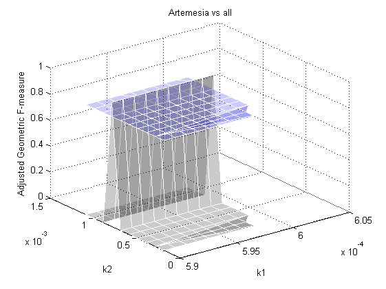
(a)

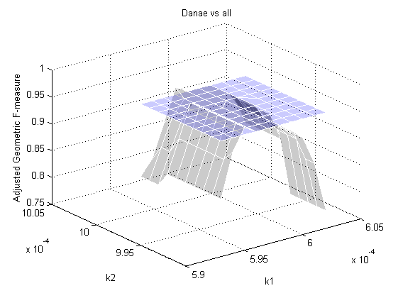
(b)

Figure 6: Parameter choice 1. The $x$ and $y$ axes represent the values of the parameters of the two methods, while on the $z$ axis is plotted the AGF for two of the OvA configurations of the dataset in (?): (a) Artemisia vs. all and (b) Danae vs. all. The gray and blue surfaces represent, respectively, the results with the AKS and SVM classifiers.

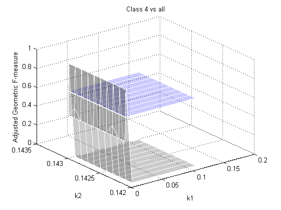
(a)

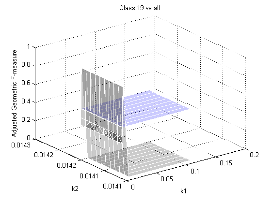
(b)

Figure 7: Parameter choice 2. The $x$ and $y$ axes represent the values of the parameters of the two methods, while on the $z$ axis is plotted the AGF for two of the OvA configurations on the dataset in (?): (a) Class 4 vs. all and (b) class 19 vs. all. The gray and blue surfaces represent, respectively, the results with the AKS and SVM classifiers.

Table 16: Comparison results on the dataset in (?) and Table 14.

AGF
Problem	AKS	C4.5	RIPPER	L2-L SVM	L2 RLR	RDR
1	0.9414	0.5614	0.8234	0.6500	0.5456	0.8987
2	0.9356	0.8256	0.6600	0.8356	0.8078	0.7245
3	0.9678	0.8462	0.8651	0.4909	0.6123	0.7654
4	0.9746	0.8083	0.6600	0.4790	0.4104	0.6693
5	0.9654	0.7129	0.9861	0.8456	0.4432	0.6134
6	0.9342	0.5714	0.9525	0.8434	0.9525	0.5554
7	0.9567	0.6151	0.7423	0.5357	0.4799	0.6151
8	0.8345	0.4123	0.3563	0.7431	0.5124	0.7124
9	0.9435	0.9456	0.9456	0.8345	0.6600	0.6600
10	0.8456	0.4839	0.5345	0.4123	0.4009	0.5456
11	0.9457	0.9167	0.9088	0.9220	0.8666	0.9132
12	0.6028	0.5875	0.5239	0.4124	0.4934	0.5234
13	0.8847	0.7357	0.6836	0.7436	0.7013	0.5712
14	0.9376	0.9376	0.8562	0.8945	0.8722	0.8320
15	0.9765	0.8630	0.8897	0.8225	0.7440	0.8630
16	0.7142	0.5833	0.3893	0.4323	0.5455	0.5111

Table 17: Comparison results on the dataset in (?) and Table 15.

AGF
Problem	AKS	C4.5	RIPPER	L2-L SVM	L2 RLR	RDR
1	0.9822	0.6967	0.5122	0.4232	0.4322	0.6121
2	0.9143	0.5132	0.4323	0.4121	0.4212	0.5323
3	0.9641	0.4121	0.4211	0.4213	0.3221	0.4323
4	0.9454	0.4332	0.1888	0.4583	0.3810	0.3810
5	0.9554	0.3810	0.2575	0.5595	0.3162	0.6967
6	0.9624	0.3001	0.1888	0.1312	0.3456	0.3121
7	0.9344	0.3810	0.5566	0.4122	0.4455	0.2234
8	0.9225	0.4333	0.1112	0.2575	0.1888	0.1888
9	0.9443	0.6322	0.1888	0.1888	0.6122	0.6641
10	0.9653	0.1897	0.5234	0.6956	0.1888	0.1121

7 Conclusions

In this paper a structure for image representation called Attributed Relational SIFT-based Regions Graph (ARSRG) is presented through description and analysis of new aspects. Starting from previous works and performing a thorough study, theoretical notions have been introduced in order to clarify and deepen the structural design of ARSRG. It has been demonstrated how ARSRG can be adopted in disparate fields such as graph matching, graph embedding, bag of graph words and kernel graph embedding with application of object recognition and art painting retrieval/classification. The experimental results have amply shown how the performances on different datasets are better than state of art competitors. Future developments certainly include exploration of additional application fields, introduction of additional algorithms (mainly graph matching) to improve performance comparison and a greater enrichment of image features to include within the ARSRG.

Acknowledgments

This work is dedicated to Alfredo Petrosino. With him I took my first steps in the field of computer science. During these years spent together, I learned firmness in achieving goals, love and passion for the work. I will be forever grateful. Thank you my great master.

References

- Acosta-Mendoza et al. Acosta-Mendoza, N., Gago-Alonso, A., & Medina-Pagola, J. E. (2012). Frequent approximate subgraphs as features for graph-based image classification. Knowledge-Based Systems, 27, 381–392.
- Alahi et al. Alahi, A., Ortiz, R., & Vandergheynst, P. (2012). Freak: Fast retina keypoint. In 2012 IEEE Conference on Computer Vision and Pattern Recognition, pp. 510–517. Ieee.
- Bay et al. Bay, H., Tuytelaars, T., & Van Gool, L. (2006). Surf: Speeded up robust features. In European conference on computer vision, pp. 404–417. Springer.
- Boser et al. Boser, B. E., Guyon, I. M., & Vapnik, V. N. (1992). A training algorithm for optimal margin classifiers. In Proceedings of the fifth annual workshop on Computational learning theory, pp. 144–152. ACM.
- Calonder et al. Calonder, M., Lepetit, V., Strecha, C., & Fua, P. (2010). Brief: Binary robust independent elementary features. In European conference on computer vision, pp. 778–792. Springer.
- Chang et al. Chang, C., Etezadi-Amoli, M., & Hewlett, M. (2009). A day at the museum..
- Chang et al. Chang, S.-F., Sikora, T., & Purl, A. (2001). Overview of the mpeg-7 standard. IEEE Transactions on circuits and systems for video technology, 11(6), 688–695.
- Chatzichristofis & Boutalis Chatzichristofis, S. A., & Boutalis, Y. S. (2008a). Cedd: color and edge directivity descriptor: a compact descriptor for image indexing and retrieval. In International Conference on Computer Vision Systems, pp. 312–322. Springer.
- Chatzichristofis & Boutalis Chatzichristofis, S. A., & Boutalis, Y. S. (2008b). Fcth: Fuzzy color and texture histogram-a low level feature for accurate image retrieval. In 2008 Ninth International Workshop on Image Analysis for Multimedia Interactive Services, pp. 191–196. IEEE.
- Cho et al. Cho, M., Lee, J., & Lee, K. M. (2010). Reweighted random walks for graph matching. In European conference on Computer vision, pp. 492–505. Springer.
- Cho & Lee Cho, M., & Lee, K. M. (2012). Progressive graph matching: Making a move of graphs via probabilistic voting. In Computer Vision and Pattern Recognition (CVPR), 2012 IEEE Conference on, pp. 398–405. IEEE.
- Cohen Cohen, W. W. (1995). Fast effective rule induction. In Machine learning proceedings 1995, pp. 115–123. Elsevier.
- Čuljak et al. Čuljak, M., Mikuš, B., Jež, K., & Hadjić, S. (2011). Classification of art paintings by genre. In 2011 Proceedings of the 34th International Convention MIPRO, pp. 1634–1639. IEEE.
- Dazeley et al. Dazeley, R., Warner, P., Johnson, S., & Vamplew, P. (2010). The ballarat incremental knowledge engine. In Pacific Rim Knowledge Acquisition Workshop, pp. 195–207. Springer.
- Deng & Manjunath Deng, Y., & Manjunath, B. (2001). Unsupervised segmentation of color-texture regions in images and video. Pattern Analysis and Machine Intelligence, IEEE Transactions on, 23(8), 800–810.
- Duchenne et al. Duchenne, O., Bach, F., Kweon, I.-S., & Ponce, J. (2011a). A tensor-based algorithm for high-order graph matching. IEEE transactions on pattern analysis and machine intelligence, 33(12), 2383–2395.
- Duchenne et al. Duchenne, O., Joulin, A., & Ponce, J. (2011b). A graph-matching kernel for object categorization. In Computer Vision (ICCV), 2011 IEEE International Conference on, pp. 1792–1799. IEEE.
- Fan et al. Fan, R.-E., Chang, K.-W., Hsieh, C.-J., Wang, X.-R., & Lin, C.-J. (2008). Liblinear: A library for large linear classification. Journal of machine learning research, 9(Aug), 1871–1874.
- Fei-Fei et al. Fei-Fei, L., Fergus, R., & Perona, P. (2007). Learning generative visual models from few training examples: An incremental bayesian approach tested on 101 object categories. Computer vision and Image understanding, 106(1), 59–70.
- Gago-Alonso et al. Gago-Alonso, A., Carrasco-Ochoa, J. A., Medina-Pagola, J. E., & Fco. Martínez-Trinidad, J. (2010). Full duplicate candidate pruning for frequent connected subgraph mining. Integrated Computer-Aided Engineering, 17(3), 211–225.
- Geusebroek et al. Geusebroek, J.-M., Burghouts, G. J., & Smeulders, A. W. (2005). The amsterdam library of object images. International Journal of Computer Vision, 61(1), 103–112.
- Haladová & Šikudová Haladová, Z., & Šikudová, E. (2010). Limitations of the sift/surf based methods in the classifications of fine art paintings. Computer Graphics and Geometry, 12(1), 40–50.
- Hori et al. Hori, T., Takiguchi, T., & Ariki, Y. (2012). Generic object recognition by graph structural expression. In Acoustics, Speech and Signal Processing (ICASSP), 2012 IEEE International Conference on, pp. 1021–1024. IEEE.
- Huang et al. Huang, J., Kumar, S., Mitra, M., Zhu, W.-J., & Zabih, R. (1997). Image indexing using color correlograms. In cvpr, Vol. 97, p. 762. Citeseer.
- Jia et al. Jia, Y., Zhang, J., & Huan, J. (2011). An efficient graph-mining method for complicated and noisy data with real-world applications. Knowledge and information systems, 28(2), 423–447.
- Kobayashi et al. Kobayashi, T., Watanabe, K., & Otsu, N. (2012). Logistic label propagation. Pattern Recognition Letters, 33(5), 580–588.
- Koffka Koffka, K. (1935). Principles of gestalt psychology..
- Lazebnik et al. Lazebnik, S., Schmid, C., & Ponce, J. (2006). Beyond bags of features: Spatial pyramid matching for recognizing natural scene categories. In 2006 IEEE Computer Society Conference on Computer Vision and Pattern Recognition (CVPR’06), Vol. 2, pp. 2169–2178. IEEE.
- Lee et al. Lee, J., Cho, M., & Lee, K. M. (2011). Hyper-graph matching via reweighted random walks. In Computer Vision and Pattern Recognition (CVPR), 2011 IEEE Conference on, pp. 1633–1640. IEEE.
- Leibe & Schiele Leibe, B., & Schiele, B. (2003). Analyzing appearance and contour based methods for object categorization. In Computer Vision and Pattern Recognition, 2003. Proceedings. 2003 IEEE Computer Society Conference on, Vol. 2, pp. II–409. IEEE.
- Liu et al. Liu, Y., Zhang, D., Lu, G., & Ma, W.-Y. (2005). Region-based image retrieval with perceptual colors. Advances in Multimedia Information Processing-PCM 2004, 931–938.
- Liu et al. Liu, Y., Zhang, D., Lu, G., & Ma, W.-Y. (2007). A survey of content-based image retrieval with high-level semantics. Pattern Recognition, 40(1), 262–282.
- Love et al. Love, B. C., Rouder, J. N., & Wisniewski, E. J. (1999). A structural account of global and local processing. Cognitive psychology, 38(2), 291–316.
- Lowe Lowe, D. G. (2004). Distinctive image features from scale-invariant keypoints. International journal of computer vision, 60(2), 91–110.
- Luo & Qi Luo, M., & Qi, M. (2011). A new method for cartridge case image mosaic. Journal of Software, 6(7), 1305–1312.
- Lux & Chatzichristofis Lux, M., & Chatzichristofis, S. A. (2008). Lire: lucene image retrieval: an extensible java cbir library. In Proceedings of the 16th ACM international conference on Multimedia, pp. 1085–1088. ACM.
- Manzo Manzo, M. (2019). Kgearsrg: Kernel graph embedding on attributed relational sift-based regions graph. Machine Learning and Knowledge Extraction, 1(3), 962–973.
- Manzo & Pellino Manzo, M., & Pellino, S. (2019). Bag of arsrg words (boaw). Machine Learning and Knowledge Extraction, 1(3), 871–882.
- Manzo et al. Manzo, M., Pellino, S., Petrosino, A., & Rozza, A. (2014). A novel graph embedding framework for object recognition. In European Conference on Computer Vision, pp. 341–352. Springer.
- Manzo & Petrosino Manzo, M., & Petrosino, A. (2013). Attributed relational sift-based regions graph for art painting retrieval. In International Conference on Image Analysis and Processing, pp. 833–842. Springer.
- Maratea & Petrosino Maratea, A., & Petrosino, A. (2011). Asymmetric kernel scaling for imbalanced data classification. In International Workshop on Fuzzy Logic and Applications, pp. 196–203. Springer.
- Maratea et al. Maratea, A., Petrosino, A., & Manzo, M. (2014). Adjusted f-measure and kernel scaling for imbalanced data learning. Information Sciences, 257, 331–341.
- Marée et al. Marée, R., Geurts, P., Piater, J., & Wehenkel, L. (2005). Decision trees and random subwindows for object recognition. In ICML workshop on Machine Learning Techniques for Processing Multimedia Content (MLMM2005).
- Matas et al. Matas, J., Chum, O., Urban, M., & Pajdla, T. (2004). Robust wide-baseline stereo from maximally stable extremal regions. Image and Vision Computing, 22(10), 761–767.
- Mikolajczyk & Schmid Mikolajczyk, K., & Schmid, C. (2004). Scale & affine invariant interest point detectors. International journal of computer vision, 60(1), 63–86.
- Mikolajczyk & Schmid Mikolajczyk, K., & Schmid, C. (2005). A performance evaluation of local descriptors. Pattern Analysis and Machine Intelligence, IEEE Transactions on, 27(10), 1615–1630.
- Morales-González et al. Morales-González, A., Acosta-Mendoza, N., Gago-Alonso, A., García-Reyes, E. B., & Medina-Pagola, J. E. (2014). A new proposal for graph-based image classification using frequent approximate subgraphs. Pattern Recognition, 47(1), 169–177.
- Morales-González & García-Reyes Morales-González, A., & García-Reyes, E. B. (2013). Simple object recognition based on spatial relations and visual features represented using irregular pyramids. Multimedia tools and applications, 63(3), 875–897.
- Morioka Morioka, N. (2008). Learning object representations using sequential patterns. In AI 2008: Advances in Artificial Intelligence, pp. 551–561. Springer.
- Nayar et al. Nayar, S. K., Nene, S. A., & Murase, H. (1996). Columbia object image library (coil 100). Department of Comp. Science, Columbia University, Tech. Rep. CUCS-006-96.
- Obdrzalek & Matas Obdrzalek, S., & Matas, J. (2002). Object recognition using local affine frames on distinguished regions. In BMVC, Vol. 2, pp. 113–122.
- Quinlan Quinlan, J. R. (2014). C4. 5: programs for machine learning. Elsevier.
- Revaud et al. Revaud, J., Lavoué, G., Ariki, Y., & Baskurt, A. (2010). Learning an efficient and robust graph matching procedure for specific object recognition. In Pattern Recognition (ICPR), 2010 20th International Conference on, pp. 754–757. IEEE.
- Romero & Cazorla Romero, A., & Cazorla, M. (2010). Topological slam using omnidirectional images: Merging feature detectors and graph-matching. In Advanced Concepts for Intelligent Vision Systems, pp. 464–475. Springer.
- Rublee et al. Rublee, E., Rabaud, V., Konolige, K., & Bradski, G. R. (2011). Orb: An efficient alternative to sift or surf.. In ICCV, Vol. 11, p. 2. Citeseer.
- Ruf et al. Ruf, B., Kokiopoulou, E., & Detyniecki, M. (2008). Mobile museum guide based on fast sift recognition. In International Workshop on Adaptive Multimedia Retrieval, pp. 170–183. Springer.
- Sanromà et al. Sanromà, G., Alquézar, R., & Serratosa, F. (2010a). Attributed graph matching for image-features association using sift descriptors. Structural, Syntactic, and Statistical Pattern Recognition, 254–263.
- Sanroma et al. Sanroma, G., Alquézar, R., & Serratosa, F. (2010b). A discrete labelling approach to attributed graph matching using sift features. In Pattern Recognition (ICPR), 2010 20th International Conference on, pp. 954–957. IEEE.
- Sanromà Güell et al. Sanromà Güell, G., Alquézar Mancho, R., Serratosa Casanelles, F., et al. (2010). Graph matching using sift descriptors-an application to pose recovery of a mobile robot., 249–254.
- Tamura et al. Tamura, H., Mori, S., & Yamawaki, T. (1978). Textural features corresponding to visual perception. IEEE Transactions on Systems, man, and cybernetics, 8(6), 460–473.
- Trémeau & Colantoni Trémeau, A., & Colantoni, P. (2000). Regions adjacency graph applied to color image segmentation. IEEE Transactions on image processing, 9(4), 735–744.
- Uray et al. Uray, M., Skocaj, D., Roth, P. M., Bischof, H., & Leonardis, A. (2007). Incremental lda learning by combining reconstructive and discriminative approaches.. In BMVC, pp. 1–10.
- Wang & Gong Wang, Y., & Gong, S. (2006). Tensor discriminant analysis for view-based object recognition. In Pattern Recognition, 2006. ICPR 2006. 18th International Conference on, Vol. 3, pp. 33–36. IEEE.
- Xia & Hancock Xia, S., & Hancock, E. (2008). 3d object recognition using hyper-graphs and ranked local invariant features. Structural, Syntactic, and Statistical Pattern Recognition, 117–126.