Advanced Variations of Two-Dimensional Principal Component Analysis for Face Recognition

Abstract

The two-dimensional principal component analysis (2DPCA) has become one of the most powerful tools of artificial intelligent algorithms. In this paper, we review 2DPCA and its variations, and propose a general ridge regression model to extract features from both row and column directions. To enhance the generalization ability of extracted features, a novel relaxed 2DPCA (R2DPCA) is proposed with a new ridge regression model. R2DPCA generates a weighting vector with utilizing the label information, and maximizes a relaxed criterion with applying an optimal algorithm to get the essential features. The R2DPCA-based approaches for face recognition and image reconstruction are also proposed and the selected principle components are weighted to enhance the role of main components. Numerical experiments on well-known standard databases indicate that R2DPCA has high generalization ability and can achieve a higher recognition rate than the state-of-the-art methods, including in the deep learning methods such as CNNs, DBNs, and DNNs.

1 Introduction

Two-Dimensional Principal Component Analysis (2DPCA) [1] and its variations (e.g., [2, 3, 4, 5, 6]) are playing an increasingly important role in the recently proposed deep learning frameworks such as 2DPCANet [7, 8]. It is always expected that 2DPCA can extract the spacial information and the best features of 2-D samples which can improve the performance of dimensional reduction. From the view of numerical linear algebra, the principle of 2DPCA is to find a subspace (called eigenfaces or features) on which the projected samples have the largest variance. The reconstruction from such projection or extraction of lower dimension is in fact the optimal low-rank approximation of the original sample. When applying 2DPCA to face recognition, we compute the eigenfaces or features based on the training set, and fairly use them to compress the training and testing samples before classification. An implicitly natural assumption is that the projected samples from the testing set still have large variance on the computed subspace. This exactly depends on the generalization ability of 2DPCA. In this paper, we will review 2DPCA and variations, and present a new relaxed 2DPCA (R2DPCA) with perfections in three aspects: abstracting the features of matrix samples in both row and column directions, being innovatively armed with generalization ability, and weighting the main components by corresponding eigenvalues. Especially, R2DPCA utilizes the label information of training data, and not only aims to enlarge the variance of projections of training samples.

The principal component analysis (PCA) [9, 10], has become one of the most powerful approaches of face recognition [11, 12, 13, 14, 15]. Recently, many robust PCA (RPCA) algorithms are proposed with improving the quadratic formulation, which renders PCA vulnerable to noises, into $L_{1}$-norm on the objection function, e.g., $L_{1}$-PCA [16], $R_{1}$-PCA [17], and PCA-$L_{1}$ [18]. Meanwhile, sparsity is also introduced into PCA algorithms, resulting in a series of sparse PCA (SPCA) algorithms [19, 20, 21, 22]. A newly proposed robust SPCA (RSPCA) [23] further applies $L_{1}$-norm both in objective and constraint functions of PCA, inheriting the merits of robustness and sparsity. Observing that $L_{2}$-, $L_{1}$-, and $L_{0}$-norms are all special $L_{p}$-norm, it is natural to impose $L_{p}$-norm on the objection or/and constraint functions, straightforwardly; see PCA-$L_{p}$ [24] and generalized PCA (GPCA) [25] for instance.

To preserve the spatial structure of face images, two dimensional PCA (2DPCA), proposed by Yang et al. [1], represents face images with two dimensional matrices rather than one dimensional vectors. The computational problems bases on 2DPCA are of much smaller scale than those based on PCA, and the difficulties caused by rank defect are also avoided in general. This image-as-matrix method offers insights for improving above RSPCA, PCA-$L_{p}$, GPCA, etc. As typical examples, the $L_{1}$-norm-based 2DPCA (2DPCA-$L_{1}$) [3] and 2DPCA-$L_{1}$ with sparsity (2DPCA$L_{1}$-S) [4] are improvements of PCA-$L_{1}$ and RSPCA, respectively, and the generalized 2DPCA (G2DPCA) [5] imposes $L_{p}$-norm on both objective and constraint functions of 2DPCA. Recently, the quaternion 2DPCA is proposed in [26] and applied to color face recognition, where the red, green and blue channels of a color image is encoded as three imaginary parts of a pure quaternion matrix. To arm the quaternion 2DPCA with the generalization ability, Zhao, Jia and Gong [27] proposed the sample-relaxed quaternion 2DPCA with applying the label information (if known) of training samples. The structure-preserving algorithms of quaternion eigenvalue decomposition and singular value decomposition can be found in [28, 29, 30, 31, 32, 33].

Linear Discriminant Analysis (LDA) is another powerful feature extraction algorithm in pattern recognition and computer vision. Since LDA often suffers from the small sample size (3S) problem, some effective approaches have been proposed, such as PCA + LDA [35], orthogonal LDA [36], LDA/GSVD [37], and LDA/QR [38]. Because of the advantages over the singularity problem and the computational cost, 2DLDA and its variants have recently attracted much attention from researchers (e.g., [39, 40, 41, 42, 43, 44]). With applying the label information, the LDA-like methods are intend to compute the discriminant vectors which maximize the ratio of the between-class distance to the within-class distance.

PCA, 2DPCA and their variations are unsupervised methods, without applying the potential or known label information of samples. Their features are calculated based on the training set and thus maximize the scatter of projected training samples. The scatter of projected testing samples are not surely optimal, and certainly, so are the whole (training and testing) projected samples. Inspired by this observation, we present a new relaxation 2DPCA (R2DPCA). This approach is a generalization of G2DPCA [5], and will reduce to G2DPCA if the label information is unknown or unused. Remark that the projection of R2DPCA does not aim to maximize the variance of training samples as 2DPCA, but intends to avoid the overfitting and to enhance the generalization ability. R2DPCA sufficiently utilizes the labels (if known) of training samples, and can enhance the total scatter of whole projected samples (see Example 4.3 for the indication). Different to the idea of LDA, R2DPCA aims to apply the label information to generate a weighting vector and to construct a weighted covariance matrix in the newly proposed approach of face recognition. Thus R2DPCA never suffers from the small sample size (3S) problem.

Our contributions are in three aspects. (1) We present a new ridge regression model for 2DPCA and variations by $L_{p}$ norm. Such model is general and abstracts features of face images from both row and column directions. With this model, 2DPCA and variations are combined with additional regularization on the solution to fit various real-world applications, with the great flexibility. (2) A novel relaxed 2DPCA (R2DPCA) is proposed with a new ridge regression model. R2DPCA has the stronger generalization ability than 2DPCA, 2DPCA-L1 2DPCAL1-S and G2DPCA. To the best of our knowledge, we are the first to introduce the label information into the 2DPCA-based algorithms. We also weight the selected principle components by corresponding eigenvalues to enhance the role of main components. (3) The R2DPCA-based approaches are presented for face recognition and image reconstruction, and their effectiveness is verified by applying them on practical face image databases. They are indicated to perform better than the deep learning methods such as DNNs, DBNs and CNNs in the numerical examples.

The rest of this paper is organized as follows. In Section 2, we recall 2DPCA, 2DPCA-L1 2DPCAL1-S and G2DPCA, and present a ridge regression model to gather them together. Their improved versions are also proposed. In Section 3, we present a new relaxed two dimensional principal component analysis (R2DPCA) and the optimal algorithms. We also present the R2DPCA-based approaches for face recognition and image reconstruction. In Section 4, we compare the R2DPCA with the state-to-the-art approaches, and indicate the efficiency of the R2DPCA . In Section 5, we sum up the contributions of this paper.

2 The General Ridge Regression Model of 2DPCA and Variations

The two-dimensional principle component analysis (2DPCA) has become one of the most popular and powerful methods in data sciences, especially in image recognition. Several deep learning frameworks, which rely hugely on the wonderful properties of 2DPCA, have achieved a high level performance in data analysis. This motivates us to develop a general model of 2DPCA and variations, providing a feasible way to embed them into artificial intelligence algorithms. In this section, we firstly present a ridge regression model of the improved 2DPCA, and then analyze the relationship of the state-of-the-art variations of 2DPCA.

2.1 A New Ridge Regression Model of Improved 2DPCA

The objective of 2DPCA is to find left and/or right orthonormal bases vectors so that the projected matrix samples have the largest scatter after projection. Suppose that there are $n$ training matrix samples $\textbf{X}_{1},\textbf{X}_{2},\ldots,\textbf{X}_{n}\in\mathbb{R}^{h\times w}$, where $h$ and $w$ denote the height and width of images, respectively. Their mean value is $\Psi=\frac{1}{n}\sum\limits_{i=1}^{n}{\bf X}_{i}$. Let ${\bf U}=[u_{1},\cdots,u_{k_{1}}]\in\mathbb{R}^{h\times k_{1}}$ and ${\bf V}=[v_{1},\cdots,v_{k_{2}}]\in\mathbb{R}^{w\times k_{2}}$ gather the left and right optimal basis vectors as columns, respectively. Then the $i$-th projected matrix sample is defined by ${\bf P}_{i}={\bf U}^{T}({\bf X}_{i}-\Psi){\bf V}$. The improved 2DPCA seeks optimal ${\bf U}$ and ${\bf V}$ that minimize the scatter of the projected matrix samples. This scatter is characterized as

$$J({\bf U},{\bf V})={\rm Tr}({\bf U}^{T}{\bf E}_{1}{\bf U})+{\rm Tr}({\bf V}^{T}{\bf E}_{2}{\bf V}),$$ (1)

where

$${\bf E}_{1}=\frac{1}{n}\sum_{i=1}^{n}({\bf X}_{i}-\Psi)({\bf X}_{i}-\Psi)^{T}\in\mathbb{R}^{h\times h},\ {\bf E}_{2}=\frac{1}{n}\sum_{i=1}^{n}({\bf X}_{i}-\Psi)^{T}({\bf X}_{i}-\Psi)\in\mathbb{R}^{w\times w},$$ (2)

denote the covariance matrices of input samples on column and row directions, respectively. Both ${\bf E}_{1}$ and ${\bf E}_{2}$ are symmetric and semi-definite matrices. Since ${\bf U}$ and ${\bf V}$ are of full column rank, ${\rm Tr}({\bf U}^{T}{\bf E}_{1}{\bf U})$ and ${\rm Tr}({\bf V}^{T}{\bf E}_{2}{\bf V})$ are nonnegative. Here, ${\rm Tr}(\cdot)$ represents the trace of a matrix. Thus, a new ridge regression model for the improved 2DPCA is proposed as

$$(\widehat{{\bf U}},\widehat{{\bf V}}) ={\rm\bf arg~{}max}~{}J({\bf U},{\bf V})$$ (3a)

$${\rm s.t.} ~{}{\bf U}^{T}{\bf U}=I_{k_{1}},~{}{\bf V}^{T}{\bf V}=I_{k_{2}}.$$ (3b)

To solve the optimal problem (3), we need compute the eigenvalue problems of ${\bf E}_{1}$ and ${\bf E}_{2}$. See Algorithm 2.1 for the detail.

Algorithm 2.1 (Improved 2DPCA).

Input $n$ matrix samples, ${\bf X}_{1},\cdots,{\bf X}_{n}\in\mathbb{R}^{h\times w}~{}(h,w\geq 1)$, and two dimensions $k_{1}$ and $k_{2}$. Output the left and right optimal bases ${\bf U}=[u_{1},\cdots,u_{k_{1}}]\in\mathbb{R}^{h\times k_{1}}$ and ${\bf V}=[v_{1},\cdots,v_{k_{2}}]\in\mathbb{R}^{w\times k_{2}}$. $(1)$ Compute the covariance matrices of training samples on column and row directions ${\bf E}_{1}$ and ${\bf E}_{2}$ as in (2). $(2)$ Compute the $k_{1}$ largest eigenvalues of $E_{1}$ and the corresponding eigenvectors, denoted as $(\lambda_{1},u_{1}),$ $\ldots,$ $(\lambda_{k_{1}},u_{k_{1}})$. Let ${\bf U}=[u_{1},\cdots,u_{k_{1}}]$. $(3)$ Compute the $k_{2}$ largest eigenvalues of ${\bf E}_{2}$ and the corresponding eigenvectors, denoted as $(\lambda_{1},v_{1}),$ $\ldots,$ $(\lambda_{k_{2}},v_{k_{2}})$. Let ${\bf V}=[v_{1},\cdots,v_{k_{2}}]$.

2.2 Improved Variations of 2DPCA and Optimal Algorithms

Based on the idea in Section 2.1, we present the improved versions of 2DPCA [1], 2DPCA-$L_{1}$ [3], 2DPCA$L_{1}$-S [4], and G2DPCA [5], whose ridge regression models are proposed in the forms of computing the first projection vector.

Without loss of generality, we assume that the training samples are mean-centered, i.e., $\frac{1}{n}\sum^{n}\nolimits_{i=1}\textbf{X}_{i}=0$; otherwise, we will replace $\textbf{X}_{i}$ by $\textbf{X}_{i}-\frac{1}{n}\sum^{n}\nolimits_{i=1}\textbf{X}_{i}$. After obtaining first $k$ left and right projection vectors $\textbf{U}=[\textbf{u}_{1},\textbf{u}_{2},\ldots,\textbf{u}_{k}]$ and $\textbf{V}=[\textbf{v}_{1},\textbf{v}_{2},\ldots,\textbf{v}_{k}]$, the $(k+1)$-th left and right projection vectors $\textbf{u}_{k+1}$ and $\textbf{v}_{k+1}$ can be calculated similarly on deflated samples:

$$\textbf{X}_{i}^{R}=\textbf{X}_{i}(\textbf{I}-\textbf{V}\textbf{V}^{T}),\ \textbf{X}_{i}^{L}=\textbf{X}_{i}^{T}(\textbf{I}-\textbf{U}\textbf{U}^{T}),$$ (4)

where $i=1,2,\ldots,n$. The ridge regression models of improved 2DPCA and variations find the first left and right projection vectors $\textbf{u}\in\mathbb{R}^{h}$ and $\textbf{v}\in\mathbb{R}^{w}$ by solving the optimization problem with equality constraints as follows.

• The improved 2DPCA:

  $$\max\limits_{\textbf{u}\in\mathbb{R}^{h},~{}\textbf{v}\in\mathbb{R}^{w}}\sum\limits^{n}_{i=1}\|\textbf{X}_{i}^{L}\textbf{u}\|_{2}^{2}+\|\textbf{X}_{i}^{R}\textbf{v}\|_{2}^{2},\ s.t.~{}\|\textbf{u}\|_{2}=1~{}{\rm and}~{}\|\textbf{v}\|_{2}=1.$$ (5)

• The improved 2DPCA-$L_{1}$:

  $$\max\limits_{\textbf{u}\in\mathbb{R}^{h},~{}\textbf{v}\in\mathbb{R}^{w}}\sum\limits^{n}_{i=1}\|\textbf{X}_{i}^{L}\textbf{u}\|_{1}+\|\textbf{X}_{i}^{R}\textbf{v}\|_{1},\ s.t.~{}\|\textbf{u}\|_{1}=1~{}{\rm and}~{}\|\textbf{v}\|_{1}=1.$$ (6)

• The improved 2DPCA$L_{1}$-S:

  $$\max\limits_{\textbf{u}\in\mathbb{R}^{h},~{}\textbf{v}\in\mathbb{R}^{w}}\sum\limits^{n}_{i=1}\|\textbf{X}_{i}^{L}\textbf{u}\|_{1}+\|\textbf{X}_{i}^{R}\textbf{v}\|_{1},\ s.t.~{}\|\textbf{u}\|_{2}=1,\|\textbf{v}\|_{2}=1,{\rm and}~{}\|\textbf{u}\|_{1},\|\textbf{v}\|_{1}\leq c,$$ (7)

  where $c$ is a positive constant.

• The improved G2DPCA:

  $$\max\limits_{\textbf{u}\in\mathbb{R}^{h},~{}\textbf{v}\in\mathbb{R}^{w}}\sum\limits^{n}_{i=1}\|\textbf{X}_{i}^{L}\textbf{u}\|_{s}^{s}+\|\textbf{X}_{i}^{R}\textbf{v}\|_{s}^{s},\ s.t.~{}\|\textbf{u}\|_{p}^{p}=1~{}{\rm and}~{}\|\textbf{v}\|_{p}^{p}=1,$$ (8)

  where $s\geq 1$ and $p>0$.

Since two independent variables in models (5)-(8) are separated, it is appropriate to solve ${\bf u}$ and ${\bf v}$ separately by optimal algorithms. Taking the improved G2DPCA (8) for instance, the first projection vector w ($={\bf u}$ or ${\bf v}$) is computed by solving the optimization problem with equality constraints:

$$\max\limits_{\textbf{w}}\sum\limits^{n}_{i=1}\|\textbf{Y}_{i}\textbf{w}\|_{s}^{s},\ s.t.\|\textbf{w}\|_{p}^{p}=1$$ (9)

where ${\bf Y}={\bf X}_{i}^{L}$ or ${\bf X}_{i}^{R}$, $s\geq 1$ and $p>0$. Depending on the value $p$, the projection vector w can be updated in two different ways. If $p\geq 1$,

$$\textbf{w}^{k+1}=\sum\limits^{n}_{i=1}\textbf{Y}_{i}^{T}[|\textbf{Y}_{i}\textbf{w}^{k}|^{s-1}\circ\texttt{sign}(\textbf{Y}_{i}\textbf{w}^{k})],$$ (10a)

$$\textbf{w}^{k+1}=|\textbf{w}^{k+1}|^{q-1}\circ\texttt{sign}(\textbf{w}^{k+1}),\ \textbf{w}^{k+1}=\frac{\textbf{w}^{k+1}}{\|\textbf{w}^{k+1}\|_{p}},$$ (10b)

where $q$ satisfies $1/p+1/q=1$, $\circ$ denotes the Hadamard product, i.e., the element-wise product between two vectors. If $0<p<1$,

$$\textbf{w}^{k+1}=\sum\limits^{n}_{i=1}\textbf{Y}_{i}^{T}[|\textbf{Y}_{i}\textbf{w}^{k}|^{s-1}\circ\texttt{sign}(\textbf{Y}_{i}\textbf{w}^{k})],$$ (11a)

$$\textbf{w}^{k+1}=|\textbf{w}^{k}|^{2-p}\circ\textbf{w}^{k+1},\textbf{w}^{k+1}=\frac{\textbf{w}^{k+1}}{\|\textbf{w}^{k+1}\|_{p}}.$$ (11b)

Notice that if the terms containing variable ${\bf u}$ are omitted, the optimal models (5)-(8) are exactly the ridge regression models of well known 2DPCA [1], 2DPCA-$L_{1}$ [3], 2DPCA$L_{1}$-S [4], and G2DPCA [5] algorithms.

3 Relaxed Two-Dimensional Principal Component Analysis

2DPCA is an unsupervised methods and overlooks the potential or known label information of samples. The abstracted features maximize the scatter of projected training samples, and are implicitly expected to maximize (not surely) the scatter of projected testing samples as well. In this section, we present a new relaxed two-dimensional principal component analysis (R2DPCA) method by $L_{p}$-norm to avoid the overfitting and to enhance the generalization ability. In large amount of experiments, R2DPCA sufficiently utilizes the labels (if known) of training samples, and can enhance the total scatter of whole projected samples. Interestingly, R2DPCA never suffers from the small sample size (3S) problem as supervised method such as LDA. Now we introduce the R2DPCA from two parts: weighting vector and objective function relaxation.

3.1 Weighting vector

Suppose that training samples can be partitioned into $m$ classes and each class contains $n_{j}$ samples:

$$\textbf{X}_{1}^{1},\cdots,\textbf{X}_{n_{1}}^{1}\ |\ \textbf{X}_{1}^{2},\cdots,\textbf{X}_{n_{2}}^{2}\ |\ \cdots\ |\ \textbf{X}_{1}^{m},\cdots,\textbf{X}_{n_{m}}^{m},$$ (12)

where $\textbf{X}_{i}^{j}$ denotes the $i$-th sample of the $j$-th class, $i=1,\ldots,n_{j}$, $j=1,\ldots,m$. Define the mean of training samples from the $j$-th class as $\Psi_{j}=\frac{1}{n_{j}}\sum\limits_{i=1}^{n_{j}}\textbf{X}_{i}^{j}\in\mathbb{R}^{h\times w},$ and the $j$-th within-class covariance matrix of the training set as $\textbf{C}_{j}=\frac{1}{n_{j}}\sum\limits_{i=1}^{n_{j}}(\textbf{X}_{i}^{j}-\Psi_{j})^{T}(\textbf{X}_{i}^{j}-\Psi_{j})\in\mathbb{R}^{w\times w},$ where $j=1,\ldots,m$, $\sum_{j=1}^{m}n_{j}=n$ and $i=1,\ldots,n_{j}$. The within-class covariance matrix $\textbf{C}_{j}$ is a symmetric and positive semi-definite matrix. Its maximal eigenvalue, denoted by $\lambda_{\max}(\textbf{C}_{j})$, represents the variance of training samples $\textbf{X}_{1}^{j},\ldots,\textbf{X}_{n_{j}}^{j}$ in the principal component. The larger $\lambda_{\rm max}(\textbf{C}_{j})$ is, the better scattered the training samples of $j$-th class are. If $\lambda_{\max}(\textbf{C}_{j})=0$ then all of training samples from the $j$-th class are same, and then the contribution of the $j$-th class to the covariance matrix of training set should be reduced. To this aim, we define a weighting vector of training classes,

$$\omega=[\omega_{1},\cdots,\omega_{m}]^{T}\in\mathbb{R}^{m},\ \omega_{j}=\frac{f(\lambda_{\rm max}(\textbf{C}_{j}))}{\sum_{i=1}^{m}f(\lambda_{\rm max}(\textbf{C}_{i}))},$$ (13)

where $\omega_{j}$ is a weighting factor of the $j$-th class with a function, $f:~{}\mathbb{R}\rightarrow\mathbb{R}^{+}$. The computation of the weighting vector is proposed in Algorithm 3.2.

Algorithm 3.2 (Weighting Vector).

Input $n$ training samples as in (12), the number of classes $m$, the number of samples in each class contains $n_{j}$ and the dimension $w$. Output the weighting vector $\omega$.   function $\omega=\texttt{weightvec}(\textbf{X}_{1},\textbf{X}_{2},\cdots,\textbf{X}_{n},m,w,n_{j})$   for $j=1,2,\cdots,m$ do      $\textbf{C}_{j}=\texttt{zeros}(w,w)$      $\textbf{M}_{j}=\frac{1}{n_{j}}(\textbf{X}_{1}^{j}+\cdots+\textbf{X}_{n_{j}}^{j})$      for $i=1,2,\cdots,n_{j}$ do         $\textbf{C}_{j}=\textbf{C}_{j}+{(\textbf{X}_{i}^{j}-\Psi_{j})}^{\prime}*(\textbf{X}_{i}^{j}-\Psi_{j})$      end for      $\textbf{C}_{j}=\textbf{C}_{j}/n_{j};$      Compute relaxation vector $\omega$ defined as in (13)   end for

3.2 Objective function relaxation

With the computed weighting vector $\omega$ in hand, we define a relaxed criterion as

$$J(\textbf{u},\textbf{v})=\gamma\textbf{G}(\textbf{u},\textbf{v})+(1-\gamma)\widetilde{\textbf{G}}(\textbf{u},\textbf{v}),$$ (14)

where $\gamma\in[0,1]$ is a relaxation parameter, $\textbf{u}\in\mathbb{R}^{h}$ and $\textbf{v}\in\mathbb{R}^{w}$ are unit vectors under $L_{p}$ norm,

$$\textbf{G}(\textbf{u},\textbf{v}) :=\sum\limits^{n}_{i=1}\|\textbf{u}^{T}(\textbf{X}_{i}-\Psi)\|_{s}^{s}+\|(\textbf{X}_{i}-\Psi)\textbf{v}\|_{s}^{s},$$ (15a)

$$\widetilde{\textbf{G}}(\textbf{u},\textbf{v}) :=\sum\limits^{m}_{j=1}\sum\limits^{n_{j}}_{i=1}\left\|\frac{\omega_{j}}{n_{j}}\textbf{u}^{T}(\textbf{X}_{i}^{j}-\Psi)\right\|_{s}^{s}+\left\|\frac{\omega_{j}}{n_{j}}(\textbf{X}_{i}^{j}-\Psi)\textbf{v}\right\|_{s}^{s}.$$ (15b)

The R2DPCA finds its first projection vectors $\textbf{u}\in\mathbb{R}^{h}$ and $\textbf{v}\in\mathbb{R}^{w}$ by solving the optimization problem with equality constraints:

$$\max\limits_{\textbf{u}\in\mathbb{R}^{h},\textbf{w}\in\mathbb{R}^{w}}J(\textbf{u},\textbf{v}),~{}~{}s.t.~{}~{}\|\textbf{u}\|_{p}^{p}=1~{}\text{and}~{}\|\textbf{v}\|_{p}^{p}=1,$$ (16)

where the criterion $J(\textbf{u},\textbf{v})$ is defined as in (14). Notice that the relaxed criterion (16) reduces to (8) if $\gamma=1$, and thus, the first projection vectors of R2DPCA and G2DPCA are the same. If first $k$ projection vectors $\textbf{U}=[\textbf{u}_{1},\textbf{u}_{2},\ldots,\textbf{u}_{k}]$ and $\textbf{V}=[\textbf{v}_{1},\textbf{v}_{2},\ldots,\textbf{v}_{k}]$ have been obtained, the $(k+1)$-th projection vectors $\textbf{u}_{k+1}$ and $\textbf{v}_{k+1}$ can be calculated similarly on the deflated samples, defined as in (4). At each iterative step, we also obtain the maximal value of the objective function,

$$f_{k} =\gamma\sum\limits^{n}_{i=1}\|\textbf{u}_{k}^{T}(\textbf{X}_{i}-\Psi)^{R}\|_{s}^{s}+\|(\textbf{X}_{i}-\Psi)^{R}\textbf{v}_{k}\|_{s}^{s}$$

$$+(1-\gamma)\sum\limits^{m}_{j=1}\sum\limits^{n_{j}}_{i=1}\left\|\frac{\omega_{j}}{n_{j}}\textbf{u}_{k}^{T}(\textbf{X}_{i}^{j}-\Psi)^{R}\right\|_{s}^{s}+\left\|\frac{\omega_{j}}{n_{j}}(\textbf{X}_{i}^{j}-\Psi)^{R}\textbf{v}_{k}\right\|_{s}^{s}.$$

Exactly, the first $k$ optimal projection vectors of R2DPCA solve the optimal problem with equality constraints:

$$\begin{array}[]{l}\{\textbf{u}_{1},\ldots,\textbf{u}_{k},\textbf{v}_{1},\ldots,\textbf{v}_{k}\}=\arg\max J(\textbf{u},\textbf{v})\\[5.0pt] \ {\rm s.t.}\ \ \left\{\begin{array}[]{l}\|\textbf{u}_{i}\|_{p}^{p}=1,~{}\|\textbf{v}_{i}\|_{p}^{p}=1,\\ \textbf{u}_{i}^{T}\textbf{u}_{j}=0,~{}\textbf{v}_{i}^{T}\textbf{v}_{j}=0~{}i\neq j,\end{array}~{}i,j=1,\cdots,k.\right.\end{array}$$ (17)

Algorithm 3.3 is presented to compute first $k$ optimal left and right projection vectors.

Now we present the relationships among the improved 2DPCA, 2DPCA$L_{1}$, 2DPCA$L_{1}$-S , G2DPCA, and R2DPCA. It is obvious that 2DPCA and 2DPCA-$L_{1}$ are two special cases of G2DPCA. 2DPCA$L_{1}$-S originates from G2DPCA with $s=1$ and $p=1$ which leads to projection vector with only one nonzero element. Then the $L_{2}$-norm constraint is employed to fix this problem, resulting in 2DPCA$L_{1}$-S. On the other hand, G2DPCA with $s=1$ and $1<p<2$ behaves like 2DPCA$L_{1}$-S, since the $L_{p}$-norm constraint in G2DPCA behaves like the mixed-norm constraint in 2DPCA$L_{1}$-S. R2DPCA is a generalization of G2DPCA.

Algorithm 3.3 (Relaxed Two-Dimensional Principal Component Analysis (R2DPCA)).

Input training samples as in (12) and parameters $s\in[1,\infty)$, $p\in(0,\infty].$   (1) Computing the weighting vector, $\omega$, by Algorithm 3.2.   (2) Compute the covariance matrix and the relaxed covariance matrix as in (15).   (3) Compute the left features $\textbf{U}=[\textbf{u}_{1},\ldots,\textbf{u}_{k}]$, the right features $\textbf{V}=[\textbf{v}_{1},\ldots,\textbf{v}_{k}]$, and the variances $\textbf{D}=\texttt{diag}(f_{1},\ldots,f_{k})$, according to the relaxed criterion (14).   for $t=1,2,\cdots,r$ do      Initialize $k=0$, $\delta=1$, arbitrary $\textbf{v}^{0}$ with $\parallel\textbf{v}^{0}\parallel_{p}=1$.      $f_{0}=J(\textbf{u}^{0},\textbf{v}^{0})$ according to (14).      while $\delta>tol$ do         $\textbf{v}^{k+1}$ is computed in the following four cases. $\textbf{u}^{k+1}$ is computed by the similar way.          $\textbf{w}^{k}=\gamma\sum\limits^{n}_{i=1}\textbf{X}_{i}^{T}[|\textbf{X}_{i}\textbf{v}^{k}|^{s-1}\circ\texttt{sign}(\textbf{X}_{i}\textbf{v}^{k})]+$              $(1-\gamma)\sum\limits^{m}_{j=1}\sum\limits^{n_{j}}_{j=1}(\frac{v_{j}}{n_{j}}\textbf{X}_{i}^{j})^{T}[|\frac{\omega_{j}}{n_{j}}\textbf{X}_{i}^{j}\textbf{v}^{k}|^{s-1}\circ\texttt{sign}(\frac{\omega_{j}}{n_{j}}\textbf{X}_{i}^{j}\textbf{v}^{k})]$.          Case 1: $0<p<1$.  $\textbf{w}^{k}=|\textbf{v}^{k}|^{2-p}\circ\textbf{w}^{k},$  $\textbf{v}^{k+1}=\frac{\textbf{w}^{k}}{\parallel\textbf{w}^{k}\parallel_{p}}.$          Case 2: $p=1$.  $j=\arg\max\nolimits_{i\in[1,w]}|w_{i}^{k}|,$  $v_{i}^{k+1}=\left\{\begin{aligned} \texttt{sign}(v_{j}^{k}),\ i=j,\\ 0,\ i\neq j.\\ \end{aligned}\right.$          Case 3: $1<p<\infty$.  $q=p/(p-1),$  $\textbf{w}^{k}=|\textbf{w}^{k}|^{q-1}\circ\texttt{sign}(\textbf{w}^{k}),$  $\textbf{v}^{k+1}=\frac{\textbf{w}^{k}}{\parallel\textbf{w}^{k}\parallel_{p}}.$          Case 4: $p=\infty$.  $\textbf{v}^{k+1}=\texttt{sign}(\textbf{w}^{k}).$         $f_{k+1}=J(\textbf{u}^{k+1},\textbf{v}^{k+1})$ according to (14).         $\delta=|f_{k+1}-f_{k}|/|f_{k}|.$         $k\leftarrow k+1.$      end while      $\textbf{U}\leftarrow[\textbf{U},\textbf{v}^{k}].$ $\textbf{V}\leftarrow[\textbf{V},\textbf{v}^{k}].$ $\textbf{D}=\texttt{diag}(\textbf{D},f_{k}).$      $\textbf{X}_{i}^{R}=\textbf{X}_{i}^{R}(\textbf{I}-\textbf{V}\textbf{V}^{T}),i=1,2,\cdots,n.$   end for

3.3 Face recognition

Suppose we have computed the optimal projections, $\widehat{{\bf U}}$ and $\widehat{{\bf V}}$, and the diagonal matrix $D$ by R2DPCA. The R2DPCA approach for color face recognition is proposed in Algorithm 3.4.

Algorithm 3.4 (R2DPCA approach for face recognition).

Input the training set, $\{{\bf X}_{1},\cdots,{\bf X}_{n}\}$, the optimal projections, $\widehat{{\bf U}}$ and $\widehat{{\bf V}}$, and the set of face images to be recognized, $\mathbb{T}=\{{\bf T}_{1},\cdots,{\bf T}_{k}\}$. Output the identity vector of $\mathbb{T}$, $r\in\mathbb{R}^{k}$. $(1)$ Compute the features of $n$ training face images under $\widehat{{\bf U}}$ and $\widehat{{\bf V}}$ as $$\widehat{{\bf X}}_{i}=\widehat{{\bf U}}^{*}({\bf X}_{i}-\Psi)\widehat{{\bf V}}\in\mathbb{H}^{k_{1}\times k_{2}},\ i=1,\cdots,n.$$ $(2)$ Compute the feature of each face images in $\mathbb{T}$, $\widehat{{\bf T}}_{j}=\widehat{{\bf U}}^{*}({\bf T}_{j}-\Psi)\widehat{{\bf V}}$. $(3)$ Solve the optimal problems $$r(j)={\bf arg~{}min}_{1\leq i\leq n}\|(\widehat{{\bf T}}_{j}-\widehat{{\bf X}}_{i})D\|$$ for $j=1,\cdots,k$.

3.4 Image reconstruction

The original digit image, ${\bf X}_{i}$, can be optimally approximated by a low-rank reconstruction from its feature, $\widehat{{\bf X}}_{i}$. Suppose that $\widehat{{\bf U}}^{\bot}\in\mathbb{R}^{h\times(h-k_{1})}$ and $\widehat{{\bf V}}^{\bot}\in\mathbb{R}^{n\times(w-k_{2})}$ are the unitary complement of $\widehat{{\bf U}}$ and $\widehat{{\bf V}}$. For $i=1,\cdots,n$, the reconstructions are defined as

$$\widehat{{\bf U}}\widehat{{\bf X}}_{i}\widehat{{\bf V}}^{T}={\bf X}_{i}+{\bf P},$$ (18)

with ${\bf P}\in\{\widehat{{\bf U}}^{\bot}(\widehat{{\bf U}}^{\bot})^{T}{\bf Z}+{\bf Z}\widehat{{\bf V}}^{\bot}(\widehat{{\bf V}}^{\bot})^{*}|{\bf Z}\in\mathbb{R}^{h\times w}\}$. Here, the mean value of samples is assumed to be zero for simplicity. The image reconstruction rate of $\widehat{{\bf U}}\widehat{{\bf X}}_{i}\widehat{{\bf V}}^{T}$ is defined as follows

$$Ratio_{s}=1-\frac{\|\widehat{{\bf U}}\widehat{{\bf X}}_{i}\widehat{{\bf V}}^{T}-{\bf X}_{i}\|_{2}}{\|{\bf X}_{i}\|_{2}}=\frac{\|{\bf X}_{i}\|_{2}-\|{\bf P}\|_{2}}{\|{\bf X}_{i}\|_{2}}.$$ (19)

Note that $\widehat{{\bf U}}\widehat{{\bf X}}_{i}\widehat{{\bf V}}^{T}$ is always a good approximation of ${\bf X}_{i}$. If $k_{1}=h$ and $k_{2}=w$, $\widehat{{\bf U}}$ and $\widehat{{\bf V}}$ are a unitary matrices and hence $Ratio_{i}=1$, which means $\widehat{{\bf U}}\widehat{{\bf X}}_{i}\widehat{{\bf V}}^{T}={\bf X}_{i}$.

4 Experiments

In this section, we present numerical experiments to compare all advanced variations of 2DPCA, including in the relaxed two-dimensional principle component analysis (R2DPCA), with the state-of-the-art algorithms. The numerical experiments are performed with MATLAB-R2016 on a personal computer with Intel(R) Xeon(R) CPU E5-2630 v3 @ 2.4GHz (dual processor) and RAM 32GB.

Example 4.1.

In this experiment, we compare R2DPCA with 2DPCA, 2DPCA-$L_{1}$, 2DPCA$L_{1}$-S, and G2DPCA on face recognition by utilizing three famous databases as follows:

• Faces95 database (1440 images from 72 subjects, twenty images per subject),

• Color FERET database (3025 images from 275 subjects, eleven images per subject),

• Grey FERET database (1400 images from 200 subjects, seven images per subject).

All of face images are cropped and resized such that each image is of 80$\times$80 size. The basic setting is that $10$ and $5$ face images of each person from Faces95 and (color or grey) FERET face databases are randomly selected out as training samples, and the remaining ones are left for testing.

We test the effect of numbers of chosen features on the recognition accuracy. Let $s$ and $p$ be fixed as the optimal parameters in Table 1. The recognition accuracies of 2DPCA, 2DPCA-L1, 2DPCAL1-S, G2DPCA and R2DPCA with different feature numbers in the range of $[1,20]$ on the grey Feret databases are shown in Figure 1. The recognition accuracies of G2DPCA and R2DPCA on the Faces95 and Color Feret databases are shown in Figure 2.

From the numerical results in Table 1 and Figures 1 and 2, we can conclude that the classification accuracies of R2DPCA are higher and more stable than 2DPCA, 2DPCA-L1, 2DPCAL1-S and G2DPCA when the number of chosen features is large. The recognition accuracies of G2DPCA and R2DPCA are the same when $k=1$, in which case neither relaxation nor weighting is necessary in G2DPCA.

Table 1: Recognition accuracies of five algorithms

Algorithms	Face95		color Feret
	$Optimalparameters$	$Accuracy$	$Optimalparameters$	$Accuracy$
2DPCA	$-$	$0.8729$	$-$	$0.5982$
2DPCA-$L_{1}$	$-$	$0.8708$	$-$	$0.5985$
2DPCA$L_{1}$-S	$\rho=-0.5$	$0.8785$	$\rho=-0.3$	$0.6236$
G2DPCA	$s=2.7,p=2.2$	$0.9451$	$s=2.8,p=2.6$	$0.6918$
R2DPCA $(\gamma=0)$	$s=1,p=2.2$	0.9493	$s=3,p=2.2$	0.7085

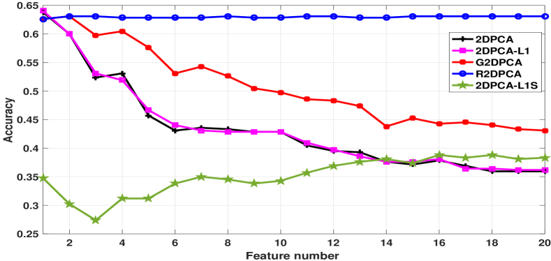
Figure 1: Recognition accuracies of 2DPCA, 2DPCA-L1, 2DPCAL1-S, G2DPCA and R2DPCA with $k=[1:20]$ on the grey FETET database.

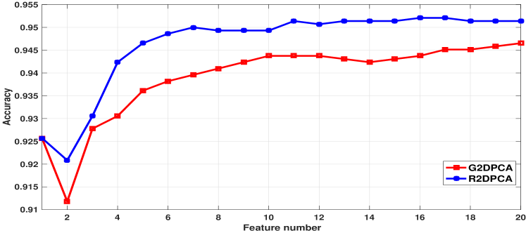
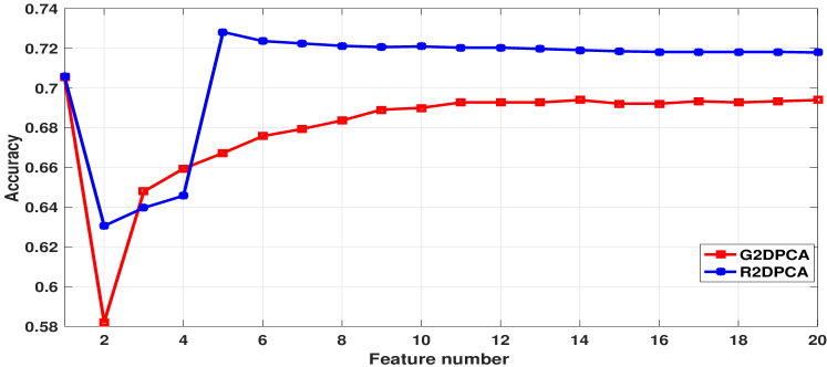
Figure 2: Recognition accuracies of R2DPCA and G2DPCA with $k=[1:20]$ on the Faces95 (top) and Color FERET (below) databases.

Example 4.2.

In this experiment, we compare R2DPCA with three most prominent deep learning primitives: Convolutional Neural Networks (CNNs), Deep Belief Networks (DBNs) and Deep Neural Networks (DNNs). These methods are applied on the partial MNIST database of handwritten digits, which has a training set of $10000$ samples, and a test set of $1000$ samples. The size of each image is $28\times 28$ pixels. The codes of CNNs, DBNs and DNNs are according to [45] and [46], and the settings are as follows.

Deep Neural Networks (DNNs) are implemented by stacking layers of neural networks along the depth and width of smaller architectures. A four-layer neural network is used in our tests. The input layer of the network contains $784=28\times 28$ neurons and the output layer contains $10$ neurons. The number of neurons in first and second hidden layers are set by $n$ and $\ell$, where $n$ increases from $1$ to $12$ and $\ell=14$ is fixed. All weights and biases are initialized randomly between $[0,1]$ and will be updated by error back propagation algorithm. The iteration will stop once the convergence condition is achieved. In our test, this condition is that if current accuracy of test samples is lower than last iteration more than three times.

Deep Belief Networks (DBNs) consist of a number of layers of Restricted Boltzmann Machines (RBMs) which are trained in a greedy layer wise fashion. The lower layer is same as the input layer in DNNs, and the top layer as the hidden layer. In our experiment, a four layers consisted of two RBMs are constructed. We set the number of hidden neurons in first RBM from $10$ to $120$, step $10$ and a fixed number of hidden neurons of $100$ in second RBM. Each RBM is trained in a layer-wise greedy manner with contrastive divergence. All weights and biases are initialized to be zero. Each RBM is trained on the full $10000$ images training set, using mini-batches of size $100$, with a fixed learning rate of $1$ for one epoch. One epoch is one full sweep of the data. Having trained the first RBM the entire training dataset is transformed through the first RBM resulting in a new $10000$ by $k$ $(k=10:10:120)$ dataset which the second RBM is trained on. Then the trained weights and biases are used to initialize a feed-forward neural net with $3$ layers of sizes $k-1000-10$, the last 10 neurons being the output label units. The feed-forward neural net is trained with sigmoid activation function using backpropagation. Here we set the mini-batches of size $100$ for one epoch using a fixed learning rate of $1$. At last the $1000$ test samples are performed in the feed-forward network and the maximum output unit are their labels.

Convolutional Neural Networks (CNNs) are feed-forward, back-propagate neural networks with a special architecture inspired from the visual system, consisting of alternating layers of convolution layers and sub-sampling layers. What is different is that CNNs work on the two dimensional data directly. In our experiment, we set two convolution layers and two sub-sampling layers. The first layer has k feature maps, where we set $k$ from $1$ to $12$, step $1$, connected to the single input layer through $k$ $5\times 5$ kernels. The second layer is a $2\times 2$ mean-pooling layer. The third layer has $12$ feature maps which are all connected to all k mean-pooling layers below through $12k$ $5\times 5$ kernels. The fourth layer is still a $2\times 2$ mean-pooling layer. After above steps the feature maps is concatenated into a feature vector which feeds into the final layer which consists of $10$ output neurons, corresponding to the $10$ class labels. The CNNs are trained with stochastic gradient descent on the training set, using mini-batches of size $50$, with a fixed learning rate of $1$ for one epoch. Putting test samples in the trained networks and comparing output with their true labels in order are to get the recognition rate.

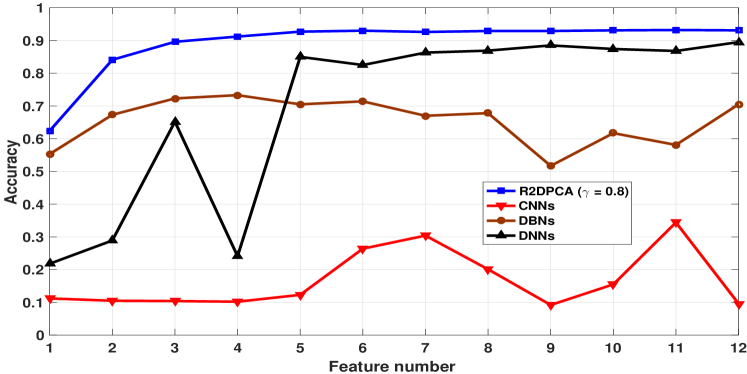
Figure 3: Recognition accuracies on the MINIST database.

The numerical results are shown in Figure 3. We can see that R2DPCA has the better performance over CNNs, DBNs and DNNs in the recognition accuracies. It should be noticed that the recognition rates of CNNs, DBNs and DNNs can not achieve at high levels with small samples, but will increase when the amount of training samples become larger.

Example 4.3.

In this experiment, we indicate the generalization ability of R2DPCA. Let $4n$ randomly generated points be equally separated into two classes (denoted as $\times$ and $\circ$, respectively). $n$ points are chosen from each class as training samples (denoted as magenta $\times$ and $\circ$ ) and the rest as testing samples (denoted as blue $\times$ and $\circ$). The principle component of $2n$ training points is computed by 2DPCA and R2DPCA. In three random cases, the computed principle components by two methods are plotted with the black lines, and the weighting vectors of R2DPCA are $[0.7082,\ 0.2918]$, $[0.5407,\ 0.4593]$ and $[0.5972,\ 0.4028]$. The variances (the larger the better) of the training set and the whole $4n$ points, under the projection of 2DPCA and R2DPCA, are shown in Table 2.

Table 2: Variances in three random cases

$4n$	Variance of training points		Variance of testing points		Variance of the whole points
	2DPCA	R2DPCA	2DPCA	R2DPCA	2DPCA	R2DPCA
$20$	${\bf 4.0757}$	$4.0161$	$2.9006$	${\bf 2.9840}$	$3.4882$	${\bf 3.5001}$
$500$	${\bf 3.7994}$	$3.7956$	$3.6619$	${\bf 3.6741}$	$3.7306$	${\bf 3.7349}$
$1000$	${\bf 3.8708}$	$3.8626$	$4.4249$	${\bf 4.4457}$	$4.1479$	${\bf 4.1541}$

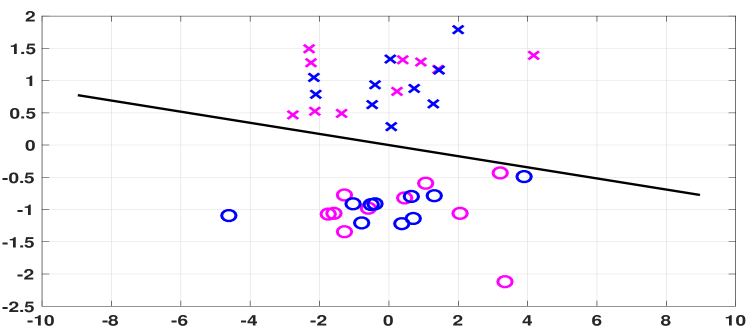
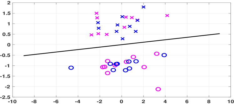
Figure 4: 2DQPCA (Top) and R2DPCA(Bellow) in random case with $n=10$: $4n$ randomly generated points are equally separated into two classes (denoted as $\times$ and $\circ$, respectively). $n$ points from each class are chosen as training samples (denoted as magenta $\times$ and $\circ$ ) and the rest as testing samples (denoted as blue $\times$ and $\circ$). The principle components of $2n$ training points are plotted with the blue lines.

5 Conclusion

This paper is a survey of recent development of 2DPCA. We present a general ridge regression model for 2DPCA and variations by $L_{p}$ norm, with the improvement on feature extraction from both row and column directions. To enhance the generalization ability, the relaxed 2DPCA (R2DPCA) is proposed with a general ridge regression model. The R2DPCA is a generalization of 2DPCA, 2DPCA-$L_{1}$ and G2DPCA, and has higher generalization ability. Since utilizing the label information, the R2DPCA can be seen as a new supervised projection method, but it is totally different to the two-dimensional linear discriminant analysis (2DLDA)[36, 39]. The R2DPCA-based approaches for face recognition and image reconstruction are also proposed and the selected principle components are weighted to enhance the role of main components. The properties and the effectiveness of proposed methods are verified by practical face image databases. In numerical experiments, R2DPCA has a better performance than 2DPCA, 2DPCA-$L_{1}$,G2DPCA, CNNs, DBNs, and DNNs.

References

References

- [1] J. Yang, D. Zhang, A. F. Frangi, J. Y. Yang (2004) Two-dimensional PCA: A new approach to appearance-based face representation and recognition, IEEE Trans. Pattern Anal. Mach. Intell., 26 (1), pp. 131-137.
- [2] Daoqiang Zhang and Zhi-Hua Zhou (2005), (2D)2PCA: Two-directional two-dimensional PCA for efficient face representation and recognition, Neurocomputing, 69(1-3), pp. 224-231.
- [3] X. Li, Y. Pang, and Y. Yuan (2010) -norm-based 2DPCA, IEEE Trans. Syst., Man, Cybern. B, Cybern., 40 (4), pp. 1170-1175.
- [4] H. Wang and J. Wang (2013) 2DPCA with -norm for simultaneously robust and sparse modelling, Neural Netw., 46, pp. 190-198.
- [5] J. Wang (2016) Generalized 2-D Principal Component Analysis by -Norm for Image Analysis, IEEE Trans. Cybern., 46 (3), pp. 792-803.
- [6] Q. Gao et al. (2019) -2-DPCA and face recognition, IEEE Trans. Cybern., 49(4), pp. 1212-1223.
- [7] D. Yu, X.-J. Wu (2017) 2DPCANet: a deep leaning network for face recognition, Multimed. Tools Appl., 4, pp. 1-16.
- [8] Y.-K. Li, X.-J. Wu, and J. Kittler (2019) L1-2D2PCANet: a deep learning network for face recognition, J. of Electronic Imaging, 28(2), pp. 023016 (20 March 2019). https://doi.org/10.1117/1.JEI.28.2.023016
- [9] I. Jolliffe (2004) Principal Component Analysis, New York, NY, USA: Springer.
- [10] M. Turk, A. Pentland (1991) Eigenfaces for recognition, J. Cogn. Neurosci., 3 (1), pp. 71-86.
- [11] L. Sirovich, M. Kirby (1987) Low-dimensional procedure for characterization of human faces, J. Optical Soc. Am. 4, pp. 519-524.
- [12] M. Kirby, L. Sirovich (1990) Application of the karhunenloeve procedure for the characterization of human faces, IEEE Trans. Pattern Anal. Mach. Intell., 12 (1), pp. 103-108.
- [13] M. Turk, A. Pentland (1991) Eigenfaces for recognition. J. Cognitive Neurosci, 3(1), pp. 71-76.
- [14] L. Zhao, Y. Yang (1999) Theoretical analysis of illumination in PCA-based vision systems, Pattern Recogn., 32(4), pp. 547-564.
- [15] A. Pentland (2000) Looking at people: sensing for ubiquitous and wearable computing, IEEE Trans. Pattern Anal. Mach. Intell., 22 (1), pp. 107-119.
- [16] Q. Ke and T. Kanade (2005) Robust norm factorization in the presence of outliters and missing data by alternative convex programming, Proc. IEEE Conf. Comput. Vis. Pattern Recognit., 1, San Diego, CA, USA, pp. 739-746.
- [17] C. Ding, D. Zhou, X. He, and H. Zha (2006) -PCA: Rotational invariant -norm principal component analysis for robust subspace factorization, Proc. 23rd Int. Conf. Mach. Learn., Pittsburgh, PA, USA, pp. 281-288.
- [18] N. Kwak (2008) Principal component analysis based on -norm maximization, IEEE Trans. Pattern Anal. Mach. Intell., 30 (9), pp. 1672-1680.
- [19] H. Zou, T. Hastie, and R. Tibshirani (2006) Sparse principal component analysis, J. Comput. Graph. Stat., 15 (2), pp. 265-286.
- [20] A. d’Aspremont, L. EI Ghaoui, M. I. Jordan, and G. R. Lanckriet (2007) A direct formulation for sparse PCA using semidefinite programming, SIAM Rev., 49 (3), pp. 434-448.
- [21] H. Shen and J. Z. Huang (2008) Sparse principal component analysis via regularized low rank matrix approximation, J. Multivar. Anal., 99 (6), pp. 1015-1034.
- [22] D. M. Witten, R. Tibshirani, and T. Hastie (2009) A penalized matrix decomposition, with applications to sparse principal components and canonical correlation analysis, Biostatistics, 10 (3), pp. 515-534.
- [23] D. Meng, Q. Zhao, and Z. Xu (2012) Improve robustness of sparse PCA by -norm maximization, Pattern Recognit., 45 (1), pp. 487-497.
- [24] N. Kwak (2014) Principal component analysis by -norm maximization, IEEE Trans. Cybern., 44 (5), pp. 594-609.
- [25] Z. Liang, S. Xia, Y. Zhou, L. Zhang, and Y. Li (2013) Feature extraction based on -norm generalized principal component analysis, Pattern Recognit. Lett., 34 (9), pp. 1037-1045.
- [26] Z. Jia, S. Ling, M. Zhao (2017) Color two-dimensional principal component analysis for face recognition based on quaternion model, LNCS, vol. 10361, pp. 177-189.
- [27] M. Zhao, Z. Jia, D. Gong (2018) Sample-relaxed two-dimensional color principal component analysis for face recognition and image reconstruction, arXiv.org/cs /arXiv:1803.03837v1, 10 Mar 2018.
- [28] Z. Jia, M. Wei, S. Ling (2013) A new structure-preserving method for quaternion Hermitian eigenvalue problems, J. Comput. Appl. Math. 239, pp. 12-24.
- [29] R. Ma, Z. Jia, Z. Bai (2018) A structure-preserving Jacobi algorithm for quaternion Hermitian eigenvalue problems, Comput. Math. Appl., 75(3), pp. 809-820.
- [30] Z. Jia, R. Ma, M. Zhao (2017) A New Structure-Preserving Method for Recognition of Color Face Images, Computer Science and Artificial Intelligence , pp. 427-432.
- [31] Z. Jia, M. Wei, M. Zhao, Y. Chen (2018) A new real structure-preserving quaternion QR algorithm, J. Comput. Appl. Math. 343, pp. 26-48.
- [32] Z. Jia, M.K. Ng, G. Song (2018) Lanczos method for large-scale quaternion singular value decomposition, Numer. Algorithms, 08 November 2018. https://doi.org/10.1007/s11075-018-0621-0
- [33] Z. Jia, M.K. Ng, and G. Song (2019) Robust Quaternion Matrix Completion with Applications to Image Inpainting, Numer. Linear Algebra Appl., DOI:10.1002/nla.2245. http://www.math.hkbu.edu.hk/ mng/quaternion.html
- [34] L. Mackey (2008) Deflation methods for sparse PCA, Proc. Adv. Neural Inf. Process. Syst., 21, Whistler, BC, Canada., pp. 1017-1024.
- [35] P.N. Belhumeur, J. Hespanda, D. Kriegeman (1997) Eigenfaces vs Fisherfaces: Recognition using class specific linear projection. IEEE Trans. Pattern Anal. Machine Intell. 19(7), pp. 711-720.
- [36] J. Ye (2005) Characterization of a family of algorithms for generalized discriminant analysis on undersampled problems, Machine Learning Res., 6, pp. 1532-4435.
- [37] P. Howland, H. Park (2004) Generalized discriminant analysis using the generalized singular value decomposition, IEEE Trans. Pattern Anal. Machine Intell. 8, pp. 995-1006.
- [38] J. Ye, Q. Li (2005) A two-stage discriminant analysis via QR decomposition, IEEE Trans. Pattern Anal. Machine Intell., 27(6), pp. 929-941.
- [39] Z.Z. Liang, Y.F. Li, P.F. Shi (2008) A note on two-dimensional linear discriminant analysis, Pattern Recognit. Lett. 29, pp. 2122-2128.
- [40] S. Kongsontana, Y. Rangsanseri (2005) Face recognition using 2DLDA algorithm, In: Proc. 8th Internat. Symp. Signal Process. Appl., pp. 675-678.
- [41] H. Xiong, M.N.S. Swamy, M.O. Ahmad (2005) Two-dimensional FLD for face recognition. Pattern Recognition 38 (7), 1121-1124.
- [42] J. Yang, J.Y. Yang, A.F. Frangi, D. Zhang (2003) Uncorrelated projection discriminant analysis and its application to face image feature extraction, Internat. J. Pattern Recognition Artificial Intell. 17 (8), pp. 1325-1347.
- [43] M. Li, B. Yuan (2005) 2D-LDA: A novel statistical linear discriminant analysis for image matrix. Pattern Recognition Lett. 26 (55), pp. 527-532.
- [44] D. Cho, U. Chang, K. Kim, B. Kim, S. Lee (2006) (2D)2DLDA for efficient face recognition. LNCS 4319, pp. 314-321.
- [45] R.B.Palm. Prediction as a candidate for learning deep hierarchical models of data.Technical University of Denmark, 2012.
- [46] M. Nielsen. Neural Networks and Deep Learning[online]. 2013. http://neuralnetworksanddeeplearning.com