A Single spark model for PSR J2144$-$3933

Abstract

The partially screened vacuum gap model (PSG) for the inner acceleration region in normal radio pulsars, a variant of the pure vacuum gap model, attempts to account for the observed thermal X-ray emission from polar caps and the subpulse drifting timescales. We have used this model to explain the presence of death lines, and extreme location of PSR J2144$-$3933 in the $P-\dot{P}$ diagram. This model requires maintaining the polar cap near a critical temperature and the presence of non-dipolar surface magnetic field to form the inner acceleration region. In the PSG model, thermostatic regulation is achieved by sparking discharges which are a feature of all vacuum gap models. We demonstrate that non-dipolar surface magnetic field reduces polar cap area in PSR J2144$-$3933 such that only one spark can be produced and is sufficient to sustain the critical temperature. This pulsar has a single component profile over a wide frequency range. Single-pulse polarimetric observations and the rotating vector model confirm that the observer’s line-of-sight traverses the emission beam centrally. These observations are consistent with a single spark operating within framework of the PSG model leading to single-component emission. Additionally, single-pulse modulations of this pulsar, including lack of subpulse drifting, presence of single-period nulls and microstructure, are compatible with a single spark either in PSG or in general vacuum gap models.

1 Introduction

The pulsar J2144$-$3933, discovered by Young et al. (1999), was the longest period ($P$=8.5 seconds), isolated, radio loud pulsar for almost two decades until recently when PSR J0250+5854 ($P$=23.5 seconds) was reported by Tan et al. (2018). Long period pulsars are rare: This can be explained by the fact that as pulsars slow down, they lose their ability to both accelerate and multiply the pair plasma responsible for radio emission (Sturrock, 1971). A rotating neutron star with large surface magnetic field ($B$) generates maximum accelerating potential $\Delta V\propto B/P^{2}$ external to the star (see e.g. Ruderman & Sutherland, 1975, hereafter RS75). The primary pair plasma, formed due to pair creation in strong surface magnetic field, is accelerated by a large $\Delta V$. This leads to further production of secondary pairs which can form dense clouds of relativistically streaming pair plasma. $\Delta V$ reduces significantly in long-period pulsars and eventually goes below a critical value where the pair creation process is suppressed. Coherent radio emission from pulsars is believed to originate in the growth of instabilities in a dense relativistically streaming pair plasma (see e.g. Melrose 1995; Usov 2002; Lyubarsky 2002). Therefore, the absence of dense pair plasma causes the emission to be switched off. It is possible to find a relation between the surface magnetic field ($B_{s}$) and the bounding period by considering the magnetic field configuration and conditions for pair creation in certain limiting cases. But observations can find estimates for only the dipolar part ($B_{d}$) of surface magnetic field. Assuming the neutron star to be a homogeneous and uniform sphere of radius $=10$ km and mass $=1.4M_{\odot}$ ($M_{\odot}$ being mass of sun) the dipolar magnetic field can be estimated as $B_{d}=6.2\times 10^{12}\sqrt{P\dot{P}}$ G, where $\dot{P}$ is the measured pulsar slowdown rate. The surface field magnitude can be related to the dipolar field as $B_{s}=bB_{d}$, where $b$ is the ratio between the two. The limiting $P$ and $B_{s}$ relation is expected to be a line in the $P-\dot{P}$ plane of the pulsar population; this is usually called the death line. Hence, any pulsar with physical parameters beyond the death line should not be observed as a radio pulsar.

Young et al. (1999) noted that PSR J2144$-$3933 is an outlier based on the then existing death line predictions (Chen & Ruderman, 1993). The pulsar could only be active at radio frequencies under very specific assumptions, either due to extremely complex $B_{s}$ or a distinctive equation of state. As a result, this pulsar was considered to present significant challenges for radio emission theories. This motivated a number of different approaches including revisiting the pair creation processes in the inner magnetosphere (Zhang et al., 2000; Arons, 2000; Gil & Mitra, 2001) and exploring the presence of special equation of states (Zhou et al., 2017). Pulsar death line estimates are highly model dependent and involve several unconstrained parameters, thereby defining a broad region in the $P$-$\dot{P}$ diagram instead of a line. This is commonly called the death valley. While investigating special equations of state, Zhou et al. (2017) concluded that a massive ($>$2$M_{\odot}$) neutron star is needed to make PSR J2144$-$3933 radio loud. Greater mass increases moment of inertia ($I$) which contributes to the surface dipolar magnetic field as $B_{d}\propto\sqrt{I/R^{6}}$, in turn raising $\Delta V$ to facilitate pair production. However, just increasing $B_{d}$ is not sufficient to account for the required pair production. Detailed studies of bright wind nebulae around young pulsars (de Jager, 2007; Kargaltsev et al., 2015) and models for excitation of coherent radio emission (RS75) require high multiplicity factor ($\kappa\sim 10^{5}$) between primary and secondary pairs. $\kappa$ increases with increasing angle between photon direction and $B_{s}$, and needs significantly smaller radius of curvature of surface fields than a purely dipolar field. Also pair cascade simulations (see e.g., Timokhin & Harding 2019) suggest that such high $\kappa$ can only be obtained when strongly non-dipolar magnetic fields exist at the neutron star surface. The above arguments advocate an increased value for the ratio $b$ between surface and dipolar fields.

Primarily, there are two classes of models that can produce pair cascades in the inner magnetosphere of a pulsar. The first is the space-charge limited flow (SCLF) where stationary charges can freely flow from the polar cap. The second involves non-stationary sparking discharge from the inner vacuum gap (IVG) where charges cannot escape the surface due to high binding energy, leading to a high parallel electric field above the polar cap. Attempts to account for the existence of PSR J2144$-$3933 using the SCLF model (e.g., Zhang et al., 2000; Arons, 2000) have not succeeded in explaining important features of radio emission such as subpulse drifting. On the other hand, sparking discharge from IVG models has been more successful in explaining a wide array of radio observations. RS75 were the first to suggest that the binding energies of surface ions are significantly high for ions to be pulled out from the polar cap, thereby facilitating the formation of IVG with strong electric fields. The IVG discharges via a number of localized sparks. As these sparks grow both radially and horizontally, a non-stationary spark-associated pair plasma flow is established along the open dipolar magnetic field lines. Radio emission from these spark-associated flows leads to the observed subpulses. The growth of instabilities in the outflowing plasma stream gives rise to coherent radio emission a few hundred kilometers above the neutron star surface. As suggested by RS75 the sparks slowly undergo $\vec{E}\times\vec{B}$ drift motions across the IVG which can be observed as drifting subpulses. The electric field in the gap separates the pair plasma, where the positrons are accelerated upwards and the backflowing electrons bombard the polar cap surface resulting in thermal X-ray emission. Gil & Mitra (2001, GM01 hereafter) revisited the formation of IVG in PSR J2144$-$3933 and demonstrated that non-dipolar magnetic field with $b\sim 50$ and radius of curvature $R_{c}\sim 10^{5}$ cm are required.

Gil et al. (2003, GMG03 hereafter) argued that the accelerating potential drop in a pure vacuum gap model is very high, exceeding 10¹³ V. As a consequence, the predicted drift speeds of sparks are much faster than the observed ones. Additionally, the pure vacuum gap model predicts temperatures of about 10⁷ K from thermal polar cap; these are also much higher compared to the observational limits. A high value of the electric field leads to overestimation of binding energy of ions in the star. Subsequent detailed calculations have shown that a strong non-dipolar magnetic field ($>$10¹³ G) is needed to bind ions to the surface and form the IVG (Jones, 1986; Medin & Lai, 2006a, b). This led GMG03 to propose the partially screened gap (PSG) model which preserves the essential features of IVG but requires a lower value of electric field due to flow of low density ions from the surface. The field anomalies resulting in strong non-dipolar surface magnetic field, which are essential for this model, can be generated by Hall-drift instabilities (Geppert et al., 2013). The decreased electric field in the PSG model naturally accounts for the observed slow drift speeds and lower polar cap temperatures (Gil et al., 2006). The PSG model has also been used to understand a number of other observational properties of radio emission, such as the anti-correlation between the periodicity of subpulse drifting and the spin-down energy loss (Basu et al., 2016), the phenomenon of mode changing (Szary et al., 2015), etc.

In this paper we intend to understand the emission properties of PSR J2144$-$3933 within the framework of the PSG model. In Sec. 2 and 3 we present highly sensitive single-pulse observations and radio emission properties of this pulsar. In Sec. 4, we discuss the PSG model in the presence of a single spark and its implications on the observed radio emission of PSR J2144$-$3933.

2 Observations

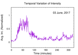
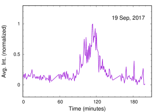
Figure 1: Variation in the single-pulse intensity of PSR J2144$-$3933 over two long observing sessions; top panel: 3 June 2017, bottom panel: 19 September 2017. Each point in these plots has been averaged over about a minute and normalised by the peak intensity. Both observations show increased intensities for 50-100 minute durations. These variations in intensity are most likely a result of diffractive scintillations.

We have used single-pulse observations from the Giant Meterwave Radio Telescope Swarup et al. (GMRT, 1991) to explore the radio emission properties of PSR J2144$-$3933. GMRT is an aperture-synthesis telescope consisting of 30 antennas distributed in a Y-shaped array with 14 antennas located within a central square-kilometer area and the remaining 16 spread along its three arms. Single-pulse observations using GMRT are usually conducted in the phased-array mode where signals from the central square antennas and the first few arm antennas are co-added in phase for increased detection sensitivities. The phase offset in each antenna is determined by observing a nearby high-intensity unresolved source, and this process is repeated roughly every one or two hours. The observations reported here were carried out using the GMRT software backend (GSB, Roy et al., 2010) (which has been superseded by the wideband uGMRT in recent years). Earlier, the GSB supported observations in several radio frequency bands with 16/32 MHz bandwidths. PSR J2144$-$3933 was observed using the GSB as part of the Meterwavelength Single pulse Polarimetric Emission Survey (MSPES, Mitra et al., 2016). MSPES conducted high sensitivity polarization measurements of single pulses in the 334 and 618 MHz frequencies using 16 MHz bandwidth. The time allotted in this survey allowed recording 325 single pulses at 334 MHz and 239 single pulses at 618 MHz for this source. In order to carry out a detailed study of single-pulse variability, newer observations of total intensity were conducted on 3 June 2017 and 19 September 2017 at 334 MHz using an increased bandwidth of 33 MHz. Around 2200 single pulses were observed on the 3 June 2017 spanning 5 hours on the source and three phasing intervals in between. An additional 1500 pulses were observed on 19 September 2017 lasting for roughly four hours and two phasing intervals in between. This newer data was recorded in filter-bank format with 256 channels and with a time resolution of 122.8 $\mu$sec (finally averaged to $\sim$1.96 msec). Post-processing of the data involved removal of spectral channels affected by radio-frequency interference, correcting the dispersion spread across channels before averaging across the entire band, and smoothing over variations across the baseline, as detailed in Basu et al. (2016).

The observed single pulses showed large intensity variations in both observing sessions (Fig. 1), with high-intensity emission was seen for roughly 50-100 minutes followed by lower-intensity signals. PSR J2144$-$3933 is a relatively nearby source with an estimated dispersion measure DM $=3.35$ pc cm^-3 and distance $d=0.16$ Kpc (Manchester et al., 1996; D’Amico et al., 1998). The observed intensity variations are most likely a result of diffractive scintillations which are propagation effects due to interaction of the pulsar emission with the interstellar medium (Rickett, 1990). The primary variabilities associated with diffractive scintillations are the decorrelation bandwidth ($\Delta\nu_{\mbox{{diss}}}$) and the diffractive timescale ($\tau_{\mbox{{diss}}}$) which can be estimated approximately using pulsar parameters. Using $\Delta\nu_{\mbox{{diss}}}$ = 11 MHz ($\nu$/GHz)^4.4(d/Kpc)^-2.2 (Cordes et al., 1985), the estimated bandwidth is $\sim$4 MHz at $\nu=0.334$ GHz and should be averaged over the observing bandwidths. The diffractive timescale is given as $\tau_{\mbox{{diss}}}$ = (A/$V_{\mbox{{iss}}}$) ($\Delta\nu_{\mbox{{diss}}}$/MHz)^0.5($\nu$/GHz)^-1 s (Cordes & Rickett, 1998), where $V_{\mbox{{iss}}}$ is the relative velocity of the pulsar. The transverse velocity of PSR J2144$-$3933 is around 120 km s^-1 which makes the diffractive timescale to be $\sim$30 mins. The estimated timescale is consistent with the intensity variations seen in Fig. 1.

3 Radio Emission Features

3.1 Stokes-I Single Pulse Modulation: Nulling and Subpulse Drifting

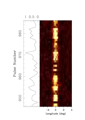
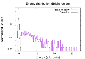
Figure 2: Nulling behaviour in PSR J2144$-$3933. Left panel: a short section of $\sim$40 pulses between pulse #945 and #985 from the start of the observation (3 June 2017) where single-period null pulses can be clearly seen. Right panel: Energy distribution (violet) of the pulse window corresponding to the bright interval between pulse #350 and #1100 during the same observing session, together with the noise distribution (black) of the baseline in the off-pulse region. The null pulses show a separate distribution overlapping the baseline histogram.

The two primary single-pulse modulations intrinsic to pulsar radio emission are the phenomena of nulling and subpulse drifting. Nulling is the sudden disappearance of emission, and ranges from short durations (few periods) to much longer stretches (hours at a time). Subpulse drifting, as discussed earlier, is the periodic modulation of subpulses within the pulse window. Nulling in PSR J2144$-$3933 was observed in MSPES, but no detailed analysis was carried out due to the relatively few pulses in the survey. Fig. 2 (left panel) shows a short pulse sequence from the observations on 3 June 2017 which shows single-period nulls. In order to characterise the nulling behaviour of this pulsar, we estimated the pulse-energy distributions from average energy across the pulse window along with the baseline distribution from the off-pulse region (Ritchings, 1976). Nulling results in a bimodal distribution of pulse energies where null pulses are overlapping with the baseline histogram. The nulling fraction identifies the relative abundance of nulling and is estimated as the ratio between the peaks of the null and the baseline distributions. As discussed earlier, the single-pulse intensities show large fluctuation in PSR J2144$-$3933 due to interstellar scintillations. In order to characterise the nulling behaviour we considered only the duration when the pulsar was in the bright state. This corresponded to around 700 pulses in the pulse range #350-#1100 for the 3 June 2017 observations whose energy histograms are shown in Fig. 2 (right panel). The null pulses are clearly seen separated from the burst distribution and we estimated the nulling fraction to be around 3.5%. In recent years, the presence of periodicity associated with nulling has been reported in a number of pulsars (Herfindal & Rankin, 2009). A standard method to estimate periodic nulling behaviour has been developed by Basu et al. (2017), where the null and bright pulses are replaced by zero and unity respectively, and then this binary series is Fourier-transformed. A similar study was conducted for the pulse sequence during the bright phase of PSR J2144$-$3933 as shown in Fig. 3 (left panel). No clear nulling-related periodicity is seen for this pulsar.

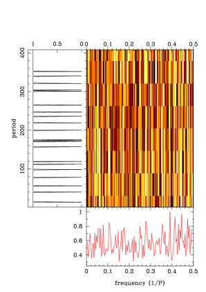
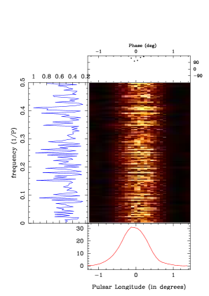
Figure 3: Periodic behaviour in single pulse sequences of PSR J2144$-$3933. Left panel: FFT power spectrum of the binary null sequence showing no signs of dominant periodicity/ies. Right panel: Longitude-resolved fluctuation spectrum (LRFS) for this pulsar showing no dominant peak (except at 0 frequency), indicating the absence of subpulse drifting.

We have also investigated the presence of subpulse drifting by using the technique of longitude-resolved fluctuation spectra (LRFS, Backer, 1973). This involves carrying out Fourier transforms along each longitude bin in the pulse window. Any periodicity will be seen as a peak in the Fourier spectrum. We have estimated the LRFS during the bright emission state of PSR J2144$-$3933 for the two long observing sessions. The LRFS was estimated for a number of different intervals ranging from 250 to 600P at a time on both observing sessions. An example of LRFS between pulse number 460 and 716 from the start of the observing session on 3 June is shown in the right panel of Fig. 3. We did not detect any periodic behaviour in this pulsar: This suggests the absence of subpulse drifting. It should be noted that any periodic behaviour longer than $\tau_{\mbox{{diss}}}$ (i.e., around 300-400$P$) will be hidden by scintillations and hence not detectable.

3.2 Polarization and Geometry

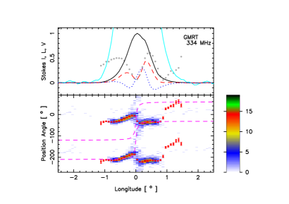
Figure 4: Polarization properties of PSR J2144$-$3933 at 334 MHz. Upper panel: Total intensity (Stokes $I$; solid curve), total linear polarization ($L$=$\sqrt{Q^{2}+U^{2}}$; dashed red), circular polarization (Stokes $V$; dotted blue), the fractional linear polarization ($L/I$; gray points), and a zoomed version of the total intensity signal ($10\times I$; cyan curve). Lower panel: The colour scale shows the single polarization position angle (PPA) contour. The average PPA traverses are plotted in red. The rotating vector model (RVM) has been used to fit the PPA traverse and is plotted twice for the two polarization modes (magenta dashed) along with the PPA. The basic parameters corresponding to the RVM fit are $\alpha=72^{\circ}$, $\beta=0.03^{\circ}$, $\phi_{\circ}=0.0^{\circ}$ and $\Psi_{\circ}=-119^{\circ}$, with the origin at the fitted PPA inflection point (see Sec. 3.2 for details).

Average profiles of PSR J2144$-$3933 are available at frequencies ranging from 334 MHz to 1.4 GHz and show a single-gaussian like shape whose width remain roughly constant for all frequencies. The estimated width measured between the outer points with 50% peak intensity ($W_{50}$) is around 0.8^∘. The polarization observations have been reported at 334 and 618 MHz in MSPES and at 667 MHz by Manchester et al. (1998). In all cases, the pulsar is seen to be strongly polarized, with percentage linear and circular polarizations to be around 30% and 5% respectively. Fig. 4 presents the average and single-pulse polarization position angle (PPA) at 334 MHz from MSPES. For each single pulse the PPAs are estimated at longitudes where the linear polarization power is more than twice the noise rms in the off pulse region. The PPA distribution from all relevant pulses is averaged within a $1\degr\times 1\degr$ cell and shown as a colour plot in bottom panel of Fig.4 (with relevant colour scale shown at the lower right of the figure). The average PPA is overplotted in red over this colour contour. Note that the PPA exhibits a fast swing across the profile. The circular polarization changes sign near the profile center as well as as towards the trailing edge of the profile. Based on these properties Manchester et al. (1998) suggested that the line of sight in this pulsar cuts the central part of the emission beam.

Alternatively, the availability of highly sensitive polarization measurements from MSPES makes it possible to assess the line of sight geometry by fitting the rotating vector model (RVM) to the PPA traverse. According to the RVM, as the star rotates and the line of sight traverses the emission region, the angle ($\Psi$) between the projected line of sight and the magnetic field vector changes as a function of pulse phase. For a star-centered dipolar magnetic field with angle $\alpha$ between the rotation axis and the magnetic axis, and angle $\beta$ between the rotation axis and the observer’s line of sight, the RVM has a characteristic S-shaped traverse given by

$$\Psi=\Psi_{\circ}+\\ \tan^{-1}\left(\frac{\sin(\alpha)\sin(\phi-\phi_{\circ})}{\sin(\alpha+\beta)\cos(\alpha)-\sin(\alpha)\cos(\alpha+\beta)\cos(\phi-\phi_{\circ})}\right)$$ (1)

where $\Psi_{\circ}$ and $\phi_{\circ}$ are the arbitrary phase offsets for the position angle $\Psi$ and longitude $\phi$ respectively. We have examined the possibility of fitting the PPA traverse of PSR J2144$-$3933 using the RVM. A jump of around 50^∘ is seen in the PPA around zero longitude which is also associated with a substantial dip in the linear polarization (Fig. 4). In the longitude range between 0^∘ and 1^∘, the PPA is continuous but shows a jump of around 80^∘ beyond the 1^∘ longitude. We fit the RVM by considering the PPA traverse in the longitude range between $-1^{\circ}$ to $1^{\circ}$ to correspond to one polarization mode, with phase-wrapping around 0^∘, while the extreme jump in PPA near the trailing edge corresponds to the orthogonal polarization mode. We have obtained a reasonable fit to the RVM but, as noted in earlier studies (e.g., von Hoensbroech & Xilouris 1997; Everett & Weisberg 2001; Mitra & Li 2004), the $\alpha$ and $\beta$ values obtained from these fits are highly correlated and unreliable. In Fig. 4, the magenta curve in the lower panel shows the RVM fits for the geometry specified by $\alpha=72^{\circ}\pm 10^{\circ}$ and $\beta=0.03^{\circ}\pm 0.01^{\circ}$. The longitude phase offsets have been subtracted and have errors of $\phi_{\circ}=0.0^{\circ}\pm 0.5^{\circ}$ and $\Psi_{\circ}=-119^{\circ}\pm 5^{\circ}$. The choice of this specific geometry can be justified as follows.

The inflexion point or steepest gradient (SG) point of the RVM occurs at the phase $\phi_{\circ}$, with the SG point being significantly better constrained by the RVM fits. The relation between different geometrical angles at the SG point is obtained from Eq. 1 as

$$\sin(\alpha)/\sin(\beta)=\mid d\Psi/d\phi\mid_{\mbox{max}}$$ (2)

In PSR J2144$-$3933 the slope has a large value $\mid d\Psi/d\phi\mid\sim 1.8\times 10^{3}$. This suggests that $\beta$ is extremely close to zero, and hence the observer cuts the pulsar beam centrally. The shape of the pulsar radio beam is most commonly represented by a central core emission surrounded by nested conal structure. The observed profile shapes with different components and classifications depend on the pulsar period, period derivative, and the line-of-sight geometry (see Rankin 1983, 1993; Mitra & Deshpande 1999; Gil & Sendyk 2000). Several careful studies have shown that the distribution of component width $W_{50}$ with respect to period has a lower boundary line which scales as $P^{-0.5}$ (Rankin, 1990; Skrzypczak et al., 2018). This scaling is similar to the opening angle of dipolar magnetic field lines. In pulsars like J2144$-$3933, with central cuts of the emission beam, the component associated with the SG point is identified as the core emission. It has been argued by Rankin (1990) that $W_{50}$ of the core at 1 GHz is related to $\alpha$ as $\sin\alpha=2.45P^{-0.5}/W_{50}$. Skrzypczak et al. (2018) confirmed the $P^{-0.5}$ scaling at lower frequencies and found the relation to be $\sin\alpha=2.39P^{-0.5}/W_{50}^{0.3GHz}$ at 0.3 GHz. The $W_{50}^{0.3GHz}$ of PSR J2144$-$3933 is 0.86^∘ which gives $\alpha\sim 72^{\circ}$. This justifies our choice of $\alpha$ in the RVM fits.

3.3 Quasiperiodic structure in Single Pulses

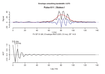
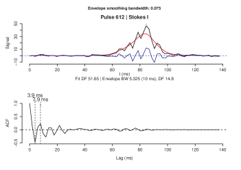
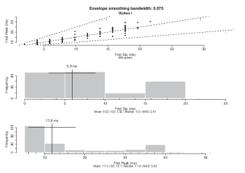
Figure 5: Analysis scheme used to infer the timescale of quasiperiodic structures in the total intensity single pulses of PSR J2144$-$3933 at 334 MHz observing frequency. The top and middle plots show two examples of these features, where the technique of Mitra et al. (2015) has been applied using a smoothing bandwidth $0.075$. The lower panel in the bottom plot represents the histograms of the estimated time scales $P_{\mu}$ of the microstructures, similar to Fig. 6 in Mitra et al. (2015). The upper panel shows the relation between the first dip and the first peak in the autocorrelation function (ACF), while the middle panel shows the distribution of the first dip in the ACF.

The subpulses in certain cases exhibit quasiperiodic structures superposed on top of a smooth emission envelope. These structures have a characteristic periodicities ($P_{\mu}$) ranging from hundreds of $\mu$sec to several msec. This quasiperiodic behaviour, commonly known as microstructure, was first observed by Craft et al. (1968) and has subsequently been seen in a large number of pulsars. A detailed and careful analysis of this phenomenon was carried out by Mitra et al. (2015) using a new method. This study includes pulsars with a wide range of periods between 100 msec and 3.5 sec, and detected such quasiperiodic structures in all four stokes parameters. The study also found a tendency of $P_{\mu}$ to increase with the pulsar period $P$ approximately as $P_{\mu}(ms)\sim 1.3\times 10^{-3}P$.

The presence of quasiperiodic structures is clearly visible in high-sensitivity total intensity measurements of single pulses of PSR J2144$-$3933 as shown in the top and middle plots of Fig. 5. We have carried out a detailed analysis of the microstructures using the analysis scheme developed by Mitra et al. (2015). The estimated $P_{\mu}$ is 7.9 msec using smoothing bandwidth $0.075$ for the two single pulses shown in Fig. 5. In order to estimate the distribution of $P_{\mu}$ we identified 355 single pulses with signal to noise ratio greater than 15 for which microstructure analysis could be carried out. A detailed quantitative analysis leads to the median $P_{\mu}=11.8\pm 6$ msec using the smoothing bandwidth $0.075$ (Fig. 5 bottom plot; see also Mitra et al., 2015). Our estimate of the microstructure timescale ($P_{\mu}=11.8\pm 6$ msec) for this pulsar ($P=8.5$ sec) is in good agreement with the consensus in the field ($P_{\mu}=11$ msec) (see also Cordes, 1979; Kramer et al., 2002).

4 The Single spark model of PSR J2144$-$3933

The polarization behaviour of PSR J2144$-$3933 suggests that its radio emission originates from open-line region of the dipolar magnetic field, with the observer’s line of sight cutting the radio emission beam centrally, and emission comprising of a single component akin to the core emission. The presence of single-period nulls and the microstructure periodicity are both consistent with the emission behaviour of normal pulsars. A number of detailed observations over the years have provided strong evidence that coherent radio emission in normal pulsars is excited by curvature radiation from charge bunches, which detaches from the pulsar magnetosphere at heights below 10% of the light-cylinder radius (for a review, see Mitra, 2017). Recent theoretical developments have also demonstrated that nonlinear growth of Langmuir waves in relativistically-moving pair plasma can result in the formation of such stable charge bunches which are capable of exciting curvature radiation in pulsars (Melikidze et al., 2000; Gil et al., 2004; Mitra et al., 2009; Melikidze et al., 2014; Lakoba et al., 2018). This essentially requires the presence of an inner acceleration region where a non-stationary relativistic flow of pair plasma can be established. A prototype for inner acceleration region is the IVG model of RS75. The IVG discharges in the form of several isolated sparks which are responsible for generating non-stationary flow of relativistic pair plasma. The growth of instabilities in the spark-associated plasma columns excite coherent curvature radiation at radio emission regions and are observed as subpulses in pulsars. The single-component emission in PSR J2144$-$3933 arises due to a single plasma column, where the polar cap size is such that only one spark can be accommodated. If the size of the actual polar cap is smaller than the fully-developed spark then the pulsar will not be radio loud. This idea was previously explored by GM01 (see also Zhang et al., 2000) within the IVG model (RS75). We will first review the ideas of GM01 before exploring the implications of single-spark in the PSG model.

There are two primary requirements for the generation of radio emission in RS75 model. The first is the formation of an IVG, and the second is facilitating conditions in IVG to generate copious amounts of pairs, their subsequent acceleration, and the cascading of pairs. The formation of the IVG is related to the problem of binding energies of electrons and ions on the stellar surface. Depending on whether $\vec{\Omega}\cdot\vec{B}>0$ or $\vec{\Omega}\cdot\vec{B}<0$, the polar cap should either be negatively charged or positively charged. RS75 argued that only in the case of $\vec{\Omega}\cdot\vec{B}<$ 0 the positive ions cannot be extracted from the stellar surface (because their binding energies are much greater than that of electrons) and the IVG can be formed. The binding energy of ions depends on the temperature of the polar cap surface as well as the surface magnetic fields. In their seminal work, RS75 overestimated the value of the binding energy and hence their estimates of potential drop above the polar cap was extremely high. Subsequently, improved calculations of binding energy were available which included the dependence on the strength of the surface magnetic fields (Jones, 1986; Medin & Lai, 2006a, b). In the literature, the estimates from Jones (1986) are widely used. Here, an empirical relationship between the equivalent temperature ($T_{i}$) of the binding energy of ions and the surface magnetic field ($B_{s}$) is given to be $T_{i}=10^{6}(B_{s}/B_{q})^{0.73}\rm{G}\approx(1.2\times 10^{5})b^{0.7}(P\dot{P}_{15})^{0.36}$ G,where $B_{q}=m^{2}c^{3}/e\hbar=4.4\times 10^{13}$ G is the critical magnetic field at which the electron gyro-frequency equals its rest mass. Thus, for strong $B_{s}$, there exists a critical temperature ($T_{i}$) such that ions cannot escape from surface and the IVG can be formed if the polar cap surface temperature $T_{s}\leq T_{i}$. The second condition for radio emission is related to the production of copious pairs and formation of sparks in the IVG. RS75 showed that the accelerating potential $\Delta V$ in the IVG is given by $\Delta V=2\pi(B_{s}/P)h^{2}$ where $h$ is the height of the gap. If $\Delta V$ falls below a critical value, sparks cannot be produced and, therefore, pulsar emission will be switched off. RS75 argued that $h$ has an upper limit $h_{\mbox{max}}\sim r_{p}$, where $r_{p}$ is the radius of polar cap. $\Delta V$ is proportionally smaller for longer-period pulsars, which ultimately results in the sparking process to stop and hence the pulsar emission to switch off.

4.1 GM01 model of IVG formation

GM01 explored the formation of IVG in presence of strong surface magnetic field and suggested the condition $T_{s}=T_{i}$, which can be expressed as critical lines in the $P-\dot{P}$ diagram. The polar cap is heated due to bombardment of backflowing electrons created during the sparking process and subsequently accelerated by $\Delta V$. It can be estimated that $T_{s}=(\kappa F)^{1/4}\left(e\Delta V\dot{N}/\sigma\pi r_{p}^{2}\right)^{1/4}$, where $\dot{N}=\pi r_{p}^{2}B_{s}/eP$ is the particle flux through the polar cap, $r_{p}=(1.4\times 10^{4})b^{-0.5}P^{-0.5}$ cm, and $\kappa F$ is a reduction parameter introduced by GM01 to accommodate for the change in speed of the bombarding particles during the spark development process. As seen above, $T_{s}$ depends on $\Delta V$ which is a function of $h$. The estimates of $h$ are dependent on models of mean free path of pair producing photons in the IVG, as well as the spark-formation process. We briefly discuss below the arguments for obtaining $h$ which are essential for the results of GM01.

In the RS75 model, the IVG discharges in the form of isolated sparks at several places by the Sturrock mechanism (Sturrock, 1971), which is described as follows: When a photon of energy in excess of 1 MeV is incident in a strong and curved magnetic field, it can split into an electron-positron pair. The large electric field in the gap causes the positrons to accelerate away from the star, while the electrons are accelerated towards the surface. These accelerating charges further radiate curvature photons; this forms additional pairs along adjacent field lines. The process continues until the whole sparking region is screened by Goldreich-Julian charge density $n_{\mbox{{gj}}}$. During this process, the size of the sparking region grows both in the vertical ($h_{\parallel}$) and horizontal ($h_{\perp}$) directions. RS75 proposed that $h_{\parallel}\approx h_{\perp}$ = $h$. The gap height is determined by the mean free path of the accelerating charge particles ($l_{\mbox{part}}$) to produce high energy photons, and the mean free path of photons ($l_{\mbox{ph}}$) before they are absorbed in magnetic field to produce pairs, i.e., $h\sim l_{\mbox{part}}+l_{\mbox{ph}}$.

GM01 noted that the formation of IVG in the normal pulsar population is possible if $0.1B_{q}<B_{s}\leq B_{q}$. In the presence of such strong magnetic fields, the near-kinematic threshold condition for pair creation is relevant. This implies that if a photon with energy greater than 1 MeV moves in super-strong magnetic fields ($>0.1B_{q}$), then after traversing a distance $l_{\mbox{ph}}\sim 2mc^{2}\Re/\hbar\omega$, pairs at or near the kinematic threshold will be produced. Here, $\omega$ is the photon frequency and $\Re$ is the radius of curvature of the magnetic field. High-energy photons can be created in the IVG by accelerating charges to Lorentz factors $\gamma$ via two distinct mechanisms, curvature radiation with characteristic frequency $\omega=(3/2)\gamma^{3}c/\Re$ or resonant inverse Compton scattering with frequency $\omega=2\gamma eB/mc$. Noting that $\gamma=e\Delta V/mc^{2}$ and using the above relations, the estimates for $h$ can be obtained in both scenarios. GM01 applied these conditions for the two cases:

1. Curvature radiation: where $l_{\mbox{part}}<<l_{\mbox{ph}}$, and hence $h=(3\times 10^{3})\Re_{6}^{2/7}b^{-4/7}P{-1/7}\dot{P}_{-15}^{-2/7}$ cm, here $\Re_{6}=\Re/10^{6}$ and $\dot{P}_{-15}=\dot{P}/10^{-15}$. Thus putting $T_{s}=T_{i}$ one can find the VG-CR family of critical line as, $\dot{P_{-15}}=2.7\times 10^{3}(\kappa F)^{1.15}\Re_{6}^{0.64}b^{-2}P^{-2.3}$ (see Eq. 10 of GM01). The next criteria for pulsar switching off arises from the condition $h_{\mbox{max}}=r_{p}/\sqrt{2}$, which gives the family of death lines for the VG-CR case as $\dot{P_{-15}}=(2.4\times 10^{-4})\Re_{6}b^{0.5}P^{4.5}$.

2. Inverse Compton scattering: $l_{\mbox{part}}\sim l_{\mbox{ph}}$, and using $l_{\mbox{part}}\sim 0.00276\gamma^{2}B_{12}^{-1}T_{6}^{-1}$ as suggested by Zhang et al. (2000), we have $h=(5\times 10^{3})\Re_{6}^{0.57}b^{-1}\dot{P}_{-15}^{-0.5}$ cm. The VG-ICS family of critical lines for vacuum gap formation using $T_{s}=T_{i}$ is given as, $\dot{P_{-15}}=2\times 10^{2}(\kappa F)^{0.7}\Re_{6}^{0.8}b^{-2}P^{-2.2}$ (see Eq. 15 of GM01). The death lines for the VG-ICS case, once again using $h_{\mbox{max}}=r_{p}/\sqrt{2}$, is estimated as $\dot{P_{-15}}=0.25\Re_{6}^{1.14}b^{-1}P^{0.28}$.

The region bounded by the line of IVG formation and death line in the $P-\dot{P}$ diagram corresponds to radio-loud pulsars. Consequently, GM01 argued that IVG can form in majority of the normal pulsars only if the surface fields are strong and non-dipolar with $b\sim 50-100$. They also showed that the VG-ICS mechanism allows more pulsars to form an IVG. Fig. 6 shows the $P-\dot{P}$ distribution of all known pulsars, where line 1 represents the VG-ICS boundary for gap formation and line 2 corresponds to the ICS death line condition as presented above (and Eq 15 and 16 of GM01). The lines use representative values of the different parameters with $b=40$, $\Re_{6}=0.1$ and $\kappa F=0.5$.

The spark formation in the RS75 model of IVG has several limitations as noted by Cheng & Ruderman (1977). Firstly, the Sturrock mechanism is difficult to realize in simple magnetic field geometries. A discharge of electron-positron pair can start at any particular magnetic field line and then progress in a certain direction without ever occurring in the original location (see Fig. 1 of Cheng & Ruderman, 1977). In the absence of repeating pairs along a particular location, it is not possible for the initial discharge to grow into a spark and locally reach Goldreich-Julian density. Cheng & Ruderman (1977) proposed a mechanism called photon splash, where a back streaming particle penetrates the stellar surface and causes a high energy ($>$1MeV) $\gamma$-ray to be emitted back in the gap region. This photon can now traverse in any direction and even produce pairs in the original field line: It is difficult to know if such a process is at work. The second limitation concerns the stability of such sparks. The development of each spark spans timescales of several tens of microseconds. On the other hand, the observed subpulses, which are believed to be associated with the spark-associated plasma columns, are seen typically for several milliseconds. This calls for a process that makes the sparks remain as stable entities for longer timescale: This is not addressed in RS75. Finally, as discussed in GMG03, the expected subpulse drift rates from the IVG model of RS75 is much faster that the observed values and, similarly, the estimated surface temperatures from this model are significantly higher than those measured from the polar cap.

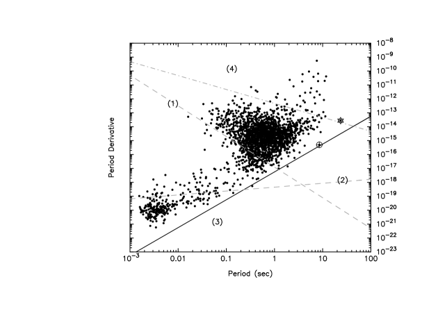
Figure 6: The $P-\dot{P}$ distribution of all known pulsars as obtained from the ATNF catalogue (Manchester et al., 2005). Lines 1 and 2 in are based on the VG-ICS model of GM01 and have been computed using the parameters $b=40$, $\Re_{6}=0.1$ and $\kappa F=0.5$ (see Sec. 4.1 for details). Line 1 corresponds to the VG-ICS line for vacuum gap formation given by $\dot{P_{-15}}=2\times 10^{2}(\kappa F)^{0.7}\Re_{6}^{0.8}b^{-2}P^{-2.2}$. Line 2 represents the VG-ICS death line condition $\dot{P}_{-15}=0.25\Re_{6}^{1.14}b^{-1}P^{0.28}$. Line 3 is our estimated death line for the PSG model and is calculated using Eq. 5 and parameters $b=40$, $\Re_{6}=0.1$, $\eta=0.1$, $T_{6}=2$ and $\alpha_{l}=45^{\circ}$. Line 4 is obtained from the higher magnetic field limit of the critical magnetic field $B_{q}=m^{2}c^{3}/e\hbar=4.4\times 10^{13}$ G beyond which the pair creation process is suppressed. The two known longest-period pulsars J2144$-$3933 (circle with cross) and J0250+5854 (star) have been explicitly identified in the plot.

4.2 PSG model and application to PSR J2144$-$3933

The possibility of steady outflow of ions from the surface of the neutron star was first suggested by Cheng & Ruderman (1977, 1980). This concept has been used by GMG03 to further develop the partially screened gap (PSG) model of the inner acceleration region. Cheng & Ruderman (1980) suggested that even if the surface of the neutron star is below $T_{i}$, there are still ions that can flow from the surface. Hence, the IVG will not exist in a purely vacuum state but will be partially filled with ions. In the PSG model, the ion charge density ($\rho_{i}$) is related to $\rho_{GJ}$ as $\rho_{i}/\rho_{GJ}\approx\exp(30-T_{i}/T_{s})$, where $\rho_{i}\leq\rho_{GJ}$ (see Eq. 8 in Cheng & Ruderman, 1980, and Eq. 1 in GMG03). If the charge density is lower than $\rho_{GJ}$ the accelerating potential in the inner accelerating region is reduced by a factor of $\eta$ such that $\Delta V_{\mbox{{psg}}}=\eta\Delta V$, where $\eta=1-\rho_{i}/\rho_{GJ}$. The exponential dependence of charge density on $T_{s}$ also makes $\Delta V_{\mbox{{psg}}}$ very sensitive to its variations; i.e., extremely small changes in $T_{s}$ can lead to large changes in the gap potential. As a result, it was proposed that the PSG is maintained in perfect thermal equilibrium with $T_{s}$ being close to $T_{i}$ (Cheng & Ruderman, 1980, GMG03). The thermal regulation can be visualized in the following manner: As soon as the temperature at a given region in the polar cap goes slightly below $T_{i}$, the accelerating potential increases and pair creation can take place which instigates the sparking process. As the spark grows, $T_{s}$ increases and hence $\eta$ continues to increase until $T_{s}=T_{i}$. At this stage, the spark terminates and the heating stops causing the surface to cool such that $T_{s}<T_{i}$, and the process repeats itself.

Let us now examine the conditions in the PSG model for the formation of a spark. The potential drop across a spark with width $h_{\perp}$ is (Szary, 2013)

$$\Delta V_{\mbox{{psg}}}=\frac{4\eta\pi bB_{d}\cos{\alpha}_{l}}{cP}h_{\perp}^{2}=\frac{4\eta bB_{d}\cos{\alpha}_{l}}{cP}A_{\mbox{sp}}.$$ (3)

Here, $A_{\mbox{sp}}=\pi h_{\perp}^{2}$ is the area of the spark and $\alpha_{l}=\alpha+\mu$ is the angle between the local magnetic field and the rotation axis, $\alpha$ is the angle between the rotation axis and the dipolar magnetic field component (see Sec. 3.2), and $\mu$ quantifies the deviation from dipole behaviour. A detailed discussion of the underlying assumptions of Eq. 3 is presented in Appendix A (see also the discussion above Eq. 16). As a result of the partial screening of the gap by factor $\eta$, the number of positrons required by the sparking process to reach Goldreich-Julian density is reduced to $\eta n_{\mbox{{gj}}}=1.4\times 10^{11}\eta(\dot{P}_{-15}/P)^{0.5}b\cos{\alpha}_{l}$. An equal number of electrons moves in the opposite direction towards the polar cap surface and supplies an energy equivalent of $L_{\mbox{part}}=q\Delta V_{\mbox{\mbox{{psg}}}}\eta n_{\mbox{{gj}}}c=\eta^{2}(\dot{P}_{-15}/P^{2})(A_{\mbox{sp}}/A_{\mbox{pc}})b\cos^{2}{\alpha_{l}}$, where $A_{\mbox{pc}}=6.58\times 10^{8}(bP)^{-1}$ cm². The condition for thermostatic equilibrium in the gap, $L_{\mbox{part}}=\sigma T^{4}$, leads to the relation

$$\frac{A_{\mbox{sp}}}{A_{\mbox{pc}}}=3.16\times 10^{-4}\frac{T_{6}^{4}}{\eta^{2}b\cos^{2}{\alpha_{l}}}\frac{P^{2}}{\dot{P}_{-15}},$$ (4)

where $T_{6}$ = $T$/10⁶ K. The sparks can only form when $A_{\mbox{sp}}\leq A_{\mbox{pc}}$. In the limiting case when $A_{\mbox{sp}}=A_{\mbox{pc}}$, the death line for the PSG model is

$$\dot{P}_{-15}=3.16\times 10^{-4}\frac{T_{6}^{4}}{\eta^{2}b\cos^{2}{\alpha_{l}}}{P^{2}}.$$ (5)

This condition for the death line obtained from the PSG model depends on a number of parameters such as $\eta$, $b$, $\alpha_{l}$ and $T_{6}$ which are not well constrained either from observations or from modeling. However, in contrast to the IVG model, photon and particle mean free paths used to estimate the gap heights and widths are no longer necessary. The IVG model requires two distinct conditions for the generation of coherent radio emission (criteria for vacuum gap formation and criteria for sparking discharge) leading to two different expressions (see Sec. 4.1). In the PSG model, both these conditions are captured in the single expression of Eq. 5.

We now investigate the conditions that will enable the single spark model (Eq. 5) to be applied to PSR J2144$-$3933. This requires making reasonable estimates for the different physical parameters in Eq. 5. The polar cap temperature and actual polar cap area can be obtained from X-ray observations modeled as blackbody spectra. PSR J2144$-$3933 is an old pulsar with characteristic age $2.7\times 10^{8}$ years and is expected to be significantly cooler than younger stars. It is possible to detect the blackbody emission from the whole star using optical observations. However, deep X-ray and optical observations have not detected any significant emission from this pulsar (Tiengo et al., 2011; Guillot et al., 2019). The upper limit for the neutron star temperature from optical observation is $4\times 10^{4}$ K (Guillot et al., 2019), while the hot polar cap temperature is lower than $1.9\times 10^{6}$ K assuming a radius of 10 m (Tiengo et al., 2011). The polar cap size requires the non-dipolar surface magnetic field to be around hundred times stronger than the dipolar value; i.e., $b\sim$ 100; and the corresponding ionic temperature is $T_{i}\approx 5\times 10^{6}$ K (Jones, 1986). A somewhat more refined estimate of $T_{i}$ as a function of $b$ is $T_{i}=1.6\times 10^{4}\left[\left(b\sqrt{P\dot{P}_{-15}}\right)^{1.07}+17.68\right]$ K (Szary, 2013; Szary et al., 2015; Medin & Lai, 2007). For PSR J2144$-$3933 parameters with $b$ = 100 once again leads to $T_{i}\approx 5\times 10^{6}$ K. There is no accurate way to calculate $T_{i}$ given the unconstrained nature of $b$. However, from the upper limits obtained above we expect $b\sim 40$. Correspondingly, $T_{i}/10^{6}=T_{6}\approx 2$ K appears to be a reasonable approximation for PSR J2144$-$3933. Next, we concentrate on constraining the screening factor in the gap. It has been shown that when $T_{i}\sim 1-2\times 10^{6}$ K and $\Re_{6}\sim 0.1-1$, then a wide range of $\eta$ between 0.1 and 0.2 is possible (see Sec. 3 and Fig. 1 in GMG03). Additionally, the subpulse drifting velocity in the PSG model is dependent on $\eta$ (see Eq. 17 in Appendix A). GMG03 and Szary (2013) used the observed drift rates for a number of pulsars and found $\eta$ to be around 0.1. Another unconstrained parameter in Eq. 5 is $\alpha_{l}$. In section 3.2 we estimated $\alpha\sim 72^{\circ}$ from polarization measurements. However, the non-dipolar field on the surface can significantly change $\alpha_{l}$ from the dipolar value by several tens of degrees (Gil et al., 2002).

We have used representative values of $\eta=0.15$, $\alpha_{l}=45^{\circ}$, $T_{6}=2$ and $b=40$ to calculate the death line of Eq. 5, which is shown in the $P-\dot{P}$ diagram of Fig. 6 (line 3 in the plot). The pulsar J2144$-$3933 has been explicitly identified in the plot (circle with cross) and is roughly coincident with the death line. This suggests that the actual polar cap size of this pulsar is such that only one fully grown spark can form. The figure also shows the longest period ($P$ = 23.5 sec) pulsar J0250+5854 (the second star-shaped point in Fig. 6) which is seen to be further away from the death line. For comparison, we have estimated $A_{\mbox{pc}}/A_{\mbox{sp}}$ from Eq. 4 using the same parameters as above and $\dot{P}_{-15}$ = 27.2 for this pulsar. The ratio $A_{\mbox{pc}}/A_{\mbox{sp}}\approx 5$, which suggests that several sparks can be formed in its polar cap and is consistent with its location away from the death line. The spark associated plasma columns results in subpulses, and it is expected that more than one component should be seen in the profile of PSR J0250+5854 (subject to line-of-sight geometry). The observed profile at 350 MHz shows the presence of two components (Fig. 6 in Tan et al., 2018), which is consistent with the predictions of the PSG model. Detailed polarization and single-pulse studies of this pulsar should provide more insights into the sparking process.

The death line in Fig. 6 (line 3) is model-dependent; i.e., each pulsar will have slightly different value of $\eta$, $B_{s}$, $\alpha_{l}$, etc. However, the known pulsar population (Fig. 6) lies above the death line predicted by the PSG model. In the higher magnetic field limit, beyond the critical magnetic field $B_{q}$ (line 4 in Fig. 6), pair creation processes are expected to be suppressed, thereby terminating the radio emission (see Usov & Melrose, 1995; Baring & Harding, 1998; Szary et al., 2014). Hence, very few radio pulsars should be seen above line 4. Most of the points in Fig. 6 above this limit correspond to anomalous X-ray pulsars which do not emit in radio frequencies. However, a few radio pulsars are still detected above this range (see e.g. Camilo et al., 2000) which cannot be explained from the present theory. There is also a potential selection bias that may result in non-detection of pulsars above line 4 (such as narrow profiles; Young et al., 1999). Line 4 is, therefore, more illustrative than a rigid boundary. In summary, the PSG model constrains the radio-loud pulsar population to lie in the region between lines 3 and 4 (Fig. 6) in the $P-\dot{P}$ diagram and, by and large, this prediction is validated by the currently known pulsar population.

4.3 Understanding the radio emission properties of PSR J2144$-$3933

We have shown that the PSG model, under reasonable assumptions, predicts a single spark operating in PSR J2144$-$3933. In the following discussion, we have used this hypothesis to understand the properties of observed radio emission described in Sec. 3.

Subpulse Drifting.

Our detailed analysis in section 3.1 indicated that PSR J2144$-$3933 shows no subpulse drifting. Here, we explore the origin of subpulse drifting within the framework of the PSG model and investigate the conditions under which it will vanish. When the temperature of the surface is slightly greater than $T_{i}$, the ions can flow freely from them. Random fluctuations in temperature can lead to conditions where $T_{s}$ goes below $T_{i}$ in certain regions, inhibiting the ion flow above it. A high potential drop quickly develops above this region whose form is given by Eq. 3. Consequently, sparking discharge is induced which continues to grow till the spark width reaches $h_{\perp}$. Typically, this takes several microseconds (see e.g. Gil & Sendyk 2000, GMG03) during which the region beneath the spark is heated due to bombardment of backflowing electrons accelerated in the gap. When the charge density in the spark reaches the Goldreich-Julian density $n_{\mbox{{gj}}}$, the temperature on the surface $T_{s}$ also increases to slightly above $T_{i}$, and the sparking process terminates. At this stage the plasma column in the gap co-rotates with the star till the gap is emptied. In this entire sparking process, the hot spot on the surface is left slightly lagging behind the co-rotation velocity. The gap emptying time is also expected to be of the order of microseconds. In contrast, the hot spot cooling time is nanoseconds (for timescale estimates see GMG03) which is several orders of magnitude lower. Since the temperature at the lagging hot spot region drops faster, the condition $T_{s}<T_{i}$ is satisfied and the region cools down, and the sparking process starts at the same lagged behind region. This lagging behind co-rotation of the hot spot region, its subsequent cooling down and regeneration of the sparking process also ensures the spark associated plasma to lag behind co-rotation as emphasized in earlier works of Basu et al. (2016); Basu & Mitra (2018); Basu et al. (2019a). The growth of plasma instabilities in the non-stationary spark-associated plasma flow results in coherent radio emission higher up in the magnetosphere. As a result, the emission also lags behind co-rotation speed and is observed as subpulse drifting.

In Appendix A, we describe in detail the general drifting behaviour in an inclined rotator using the PSG model. We see clearly that during the time in which the spark develops and attains $n_{\mbox{{gj}}}$, the plasma is lagging behind the co-rotation of the neutron star (Eq. 14). It is possible to measure the drifting periodicity ($P_{3}$) which corresponds to the time taken by the sparks to repeat at any pulse phase (Szary, 2013; Basu et al., 2016). A detailed study of the drifting behaviour was carried out by Basu et al. (2016), where using predictions from the PSG model a dependence of $P_{3}$ on observable parameters was obtained. It was shown that $P_{3}^{\mbox{{psg}}}\approx 2(\gamma_{6}/\xi_{-3})(\dot{E}/(4\times 10^{31}))^{-0.5}P$, where $\gamma_{6}\sim\gamma/10^{6}$ is the Lorentz factor of the primary particles formed in sparks, $\xi_{-3}=\xi/10^{-3}$ can be related to the efficiency of non-thermal emission and obtained from X-ray observations, and $\dot{E}$ is the spin-down energy loss expressed in erg s^-1. The $P_{3}-\dot{E}$ dependence is an important relationship because it can be verified through observations. However, measurements of $P_{3}$ are fundamentally uncertain due to the aliasing effect, where observationally it is impossible to differentiate between $P_{3}$ ($>2P$) and its aliased value $P_{3}^{{}^{\prime}}=P_{3}/(P_{3}$-1) ($P<P_{3}^{{}^{\prime}}<2P$). A physical model is essential to disentangle $P_{3}$ and $P_{3}^{{}^{\prime}}$, and the lagging behind co-rotation speed for the subpulses in PSG model allows a resolution to the aliasing effect. The lagging subpulses are expected to move from the leading to the trailing edge of the pulse window. This implies that negative drifting, where subpulses shift towards the leading part of the profile in subsequent periods, has $P_{3}>2P$, while positive drifting, with subpulses shifting towards the trailing edge, has $P<P_{3}<2P$. A comprehensive observational campaign has been conducted to measure drifting in the pulsar population by Basu et al. (2016, 2019a). It was found that drifting is limited to pulsars with $\dot{E}<2.3\times 10^{32}$ erg s^-1. The measured $P_{3}$, using the above model, has a certain spread but is anti-correlated with $\dot{E}$, given as $P_{3}^{\mbox{{obs}}}\approx(\dot{E}/(2.3\times 10^{32}))^{-0.6}P$. This shows that the PSG model of subpulse drifting is consistent with observations.

The pulsar J2144$-$3933 has $\dot{E}$ = 3.18$\times 10^{28}$ erg s^-1, and is expected to show negative drifting with subpulses moving from the trailing to the leading edge of the profile at subsequent periods.The expected periodicity of drifting from the PSG model is $P_{3}^{\mbox{{psg}}}\sim 70P$, and that estimated from the observational fits is $P_{3}^{\mbox{{obs}}}\sim 205P$. The variations between the two can be explained from the scatter in the observational measurements of $P_{3}$ as well as the uncertainty in estimating the parameter $\xi$ (Kargaltsev et al., 2012; Shibata et al., 2016). As reported in section 3.1 we have not detected the presence of drifting. There is a possibility that the drifting maybe hidden by the scintillation timescale ($\geq 400P$), but this is relevant only in case of most extreme estimates of $P_{3}$. We suggest that the absence of subpulse drifting in PSR J2144$-$3933 is due to the presence of a single spark in a small polar cap with limited space. If the polar cap is significantly larger than the spark size, several sparks can form in a closely packed manner, where the whole pattern lags behind co-rotation motion. In these cases, there is sufficient space for the sparks to continuously form as well as move across the polar cap to exhibit subpulse drifting. However, for PSR J2144$-$3933, once the spark is fully formed, it fills the whole polar cap and there is no further space for it to move across. The spark terminates and is regenerated at the same place. We further conjecture that lack of drifting in certain pulsars can arise due to conditions in the polar cap which inhibit sparks to move across it.

Nulling.

In Sec. 3.1, we found PSR J2144$-$3933 predominantly shows single-period nulls. The pulse window, in this case, is approximately 2° wide in longitude, corresponding to roughly 50 msec in time, which is the minimum time duration for the radio emission to switch off during nulling. The presence of one single spark in this pulsar also rules out the possibility that the short nulls results from the line of sight passing between empty regions of the sparking system (see e.g. Herfindal & Rankin, 2009). The empty line of sight argument for short-duration nulls have been considerably weakened by exhaustive studies showing their presence in the core component (Basu et al., 2017; Basu & Mitra, 2018; Basu et al., 2019b). This leaves two extreme possibilities: Either (a) the plasma flow entirely stops, or (b) the plasma flow is maintained but the conditions for coherent radio emission break down. According to the PSG model, the first case (a) corresponds to $T_{s}<T_{i}$, and it is difficult to envisage this condition to hold for several milliseconds. Even if it is possible to have $T_{s}<T_{i}$ for millisecond durations, the high-energy gamma-ray photons from the diffuse background can easily create pairs in the region above the polar cap within a few microseconds (see Shukre & Radhakrishnan, 1982). Hence, it is highly unlikely that the plasma flow is stopped for the duration of the nulls. The second alternative (b) implies that the thermostatic regulation of the PSG is maintained, but the nature of the non-stationary plasma flow is modified. This requires the pair-creation properties to change: In principle, this allows certain possibilities such as short-term change in the structure of the non-dipolar surface magnetic field, etc. However, at present, we are unaware of any model that can explain such changes at timescales of milliseconds to seconds.

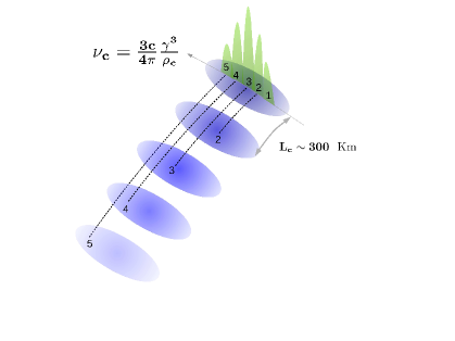
Figure 7: A cartoon illustration of how the quasiperiodic structures arise in subpulses. The blue regions correspond to five strong emission sources which are moving relativistically along the open field lines. The separation between adjacent regions as well as their physical extent is given by $L_{c}=c\Delta t$. For the typical value $\Delta t\sim 1$ msec, we get $L_{c}\sim 300$ km. Radio emission originates from a specific height due to curvature radiation with a characteristic frequency ($\nu_{c}$). The five regions identified in the figure cross this emission height sequentially, separated by $\Delta t$ in time, are detected in the emission window as separate peaks, and the empty regions between them are seen as dips in the intensity pattern. Due to the rotation of the pulsar, each emission source is observed at delayed phases within the pulse window. The linear relation of modulation periodicity $P_{\mu}$ with pulsar period $P$ suggests that the length scale $L_{c}$ remains constant for different pulsars.

Quasiperiodic structures.

As seen in Fig. 5, PSR J2144$-$3933 has the presence of modulating, quasiperiodic structures in its subpulses. This effect is seen in several pulsars and, when such modulating structures are clearly resolved, the periodicity of modulation $P_{\mu}$ is proportional to the pulsar period $P$ as $P_{\mu}\approx 10^{-3}P$ as shown in Mitra et al. (2015). This study suggested that such radiation patterns can result from the temporal modulations of non-stationary plasma flow, associated with the sparking process in the vacuum-gap class of models. Coherent radio emission is believed to be excited due to curvature radiation from charge bunches at regions below 10% of the light cylinder (Gil et al., 2004; Mitra et al., 2009; Mitra, 2017; Lakoba et al., 2018). The characteristic frequency of emission is $\nu_{c}=(3/4\pi)\gamma^{3}c/\rho_{c}$, where $\gamma$ is the Lorentz factor of the charge bunch and $\rho_{c}$ is the radius of curvature of the field lines. Since $\gamma$ does not change significantly and the emission arises from regions of dipolar magnetic field lines, radio emission at any given frequency arises from a narrow range of heights. The quasiperiodic structure seen across any subpulse should also arise from this narrow region. The origin of these microstructures can be understood under the assumption that there is a constant stream of modulating radiation patterns with lateral angular dimension equivalent to the subpulse width moving relativistically along the open magnetic field flux tubes. The radial lengths of these structures are a few hundred kilometers which are separated from each other by distinct empty regions. As the pulsar rotates, our line of sight encounters these alternating emitting structures followed by the relatively empty spaces between them at different phases of the subpulse, resulting in the observed modulating emission pattern. In Fig. 7, we present a schematic diagram to aid the visualization of a steady stream of emitting regions observed as microstructures. The period dependence of the modulation periodicity can be explained if we assume that the radial dimensions of these emitting regions remain unchanged across the pulsar population.

The single-spark PSG model for PSR J2144$-$3933 shows the sparking to be a result of the single stream of outflowing plasma, which provides a simplified window into its IAR. According to RS75, the gap height in the IAR is around 100 meters. The sparking process in the gap region lasts for a few tens of microseconds during which the $n_{\mbox{{gj}}}$ charge density is attained. Subsequently, the gap empties within about half a microsecond resulting in a spark-associated plasma column. The radial dimension of this plasma cloud is around three kilometers and it moves relativistically outward from the stellar surface along the open field lines. The separation between adjacent clouds corresponding to the gap-emptying time is around hundred meters. In steady state, just above the gap region, a non-stationary flow of plasma is established. Each plasma cloud has a distribution of particle speeds. During their outward motion, the low and high velocities of the clouds overlap at a certain height, leading to a two-stream instability and the growth of plasma waves. For strong growth of plasma waves the system can be driven to nonlinear regimes, where charge bunches can excite coherent curvature radiation. Depending on the growth and decay of plasma waves, bright and weak radio emission patterns can be generated. However, the timescales associated with these patterns are around several microseconds, corresponding to the plasma cloud sizes, and cannot explain the typical millisecond variations associated with the quasiperiodic structures. Additional physical processes resulting in variations of the sparking processs over timescales of milliseconds are required to explain the observed quasiperiodic structures which are currently unknown. Our estimates require such variations to span over typical length scales of 300 km, as illustrated in Fig. 7.

In the PSG model, the non-stationary flow is expected to be established in a manner similar to the prescription of RS75. However, the screening potential will modify the gap height and consequently the length of the instability region and the cloud overlap timescales. A detailed study of the spark development process in the PSG combined with the growth of plasma instability in the radio emission region is needed to get estimates of the cloud size and instability region timescales. Such estimates is currently unavailable, however it is still unlikely that the modified timescales from the PSG model will be sufficient to explain the millisecond quasiperiodic structures and additional physical processes will still be needed.

5 Summary

We have estimated a new death line in the $P-\dot{P}$ diagram of the pulsar population using the single-spark PSG model (Eq. 5). Our death line also explains the scarcity of long-period pulsars, contradicting the earlier predictions of GM01. Specifically, we show that this model is able to explain the radio-loudness of PSR J2144$-$3944 as being located very close to this boundary, and that the radio emission properties of PSR J2144$-$3944 are consistent with this model. Our study provides strong support for theoretical models which predict an inner acceleration region in radio pulsars where the sparking process just above the polar cap results in a nonstationary relativistic plasma flow essential for the generation of coherent radio emission.

Appendix A Golreich Julian Density and Subpulse drift direction and Speed in PSG model

In a slowly rotating neutron star system we consider two frames of reference, primed and unprimed, where the primed correspond to the co-rotating frame located at the neutron star surface, and the unprimed to the observer frame. For slow rotation, the velocity at the neutron star surface is significantly less than the velocity of light and hence the two frames can be considered as inertial frames. In this case the components of the electric field between the two frames is transformed as

$$\vec{E^{\prime}}=\vec{E}+\frac{1}{c}\left(\vec{\Omega}\times\vec{r}\right)\times\vec{B}$$ (6)

Here $\vec{\Omega}$ is the rotation vector, $\vec{r}$ is the radial vector and $\vec{B}$ is the magnetic field. Since above the polar cap the quantity $\Omega r/c$ is negligible, then the term $\delta B/\delta t\sim 0$, and thus the maxwell equations in the gap region are mainly guided by electrostatics. If the charge density is given by $\rho(r,\theta,\phi)$ then the Gauss law and Faraday’s law respectively can be written as,

$$\mathbf{div}{\vec{E^{\prime}}}=4\pi\rho(r,\theta,\phi)+\mbox{\boldmath$\nabla$}\cdot\left(\frac{1}{c}(\vec{\Omega}\times{\vec{r}})\times\vec{B}\right)$$ (7)

$$\mathbf{curl}{\vec{E^{\prime}}}=0$$ (8)

Applying appropriate boundary condition the electric field ${\vec{E^{\prime}}}=0$, when $\rho(r,\theta,\phi)=\rho_{GJ}=-1/(4\pi)\mbox{\boldmath$\nabla$}\cdot\left(\frac{1}{c}(\vec{\Omega}\times{\vec{r}})\times\vec{B}\right)$. Further if one assumes that in the polar cap region $B_{\theta}=B_{\phi}=0$ and $B_{r}\neq 0$, which is generally a very good assumption for both dipolar and non-dipolar magnetic fields, then one gets the usual form of the Goldreich Julian density as,

$$\rho_{GJ}=-\frac{\vec{\Omega}\cdot\vec{B}}{2\pi c}$$ (9)

Note in Eq.  7 the term in the left hand side can be simplified as $((\vec{\Omega}\times{\vec{r}})\times\vec{B})=\vec{r}\cdot(\vec{\Omega}\cdot\vec{B})-\vec{\Omega}\cdot(\vec{r}\cdot\vec{B})$. For the case $B_{\theta}=B_{\phi}=0$ and $B_{r}\neq 0$, this becomes $((\vec{\Omega}\times{\vec{r}})\times\vec{B})=(r\Omega B_{r}\sin\theta)\vec{\theta}$, here $\vec{\theta}$ is the unit vector. Now applying the divergence theorem to Eq.  7 one gets,

$$\iint\limits_{S}{{\vec{E^{\prime}}}}dS=4\pi\iiint\limits_{V}\rho(r,\theta,\phi)dV+\frac{1}{c}\iint\limits_{S}(r\Omega B_{r}\sin\theta\cdot\hat{\theta})dS$$ (10)

Now replacing $\rho=\rho_{GJ}-\Delta\rho$, and rearranging the equation one can write,

$$\iint\limits_{S}({{\vec{E^{\prime}}}}-\frac{1}{c}(r\Omega B_{r}\sin\theta\cdot\hat{\theta}))dS=4\pi\iiint\limits_{V}(\rho_{GJ}-\Delta\rho)dV$$ (11)

We can now write $\vec{{E^{\prime}}}=E^{\prime}_{r}\hat{r}+E^{\prime}_{\theta}\hat{\theta}+E^{\prime}_{\phi}\hat{\phi}$. Let us now consider volume element such that one side touches the wall of vacuum gap and also note that $E^{\prime}_{\phi}=0$. We also make the reasonable assumption that $E^{\prime}_{r}$ does not change significantly across the gap which gives $\iint\limits_{S}E^{\prime}_{r}ds=0$. Thus Eq. 11 can now be written as,

$$\iint\limits_{S}({{{E^{\prime}_{\theta}\hat{\theta}}}}-\frac{1}{c}(r\Omega B_{r}\sin\theta\cdot\hat{\theta}))dS=4\pi\iiint\limits_{V}(\rho_{GJ}-\Delta\rho)dV$$ (12)

We can now consider two extreme cases, one where $\rho=\rho_{GJ}$ such that $\Delta\rho=0$. In this case as per Eq. 12 , $E^{\prime}_{\theta}=0$, and this means that the entire electric field in the co-rotating frame is screened and this correspond to the case of perfect co-rotation of the charges in the IVG. Next we consider the case where $\rho=0$ or $\Delta\rho=\rho_{GJ}$. In this case, $E^{\prime}_{\theta}=(1/c)r\Omega B_{r}\sin\theta$, which means that there is full electric field available in the IVG, and hence a test charge will appear to be lag behind the rotation in the co-rotating frame and remain at rest in the observer frame. For any intermediate case,

$$\iint\limits_{S}{{{E^{\prime}_{\theta}\hat{\theta}}}}dS=-4\pi\iiint\limits_{V}\Delta\rho dV$$ (13)

$E^{\prime}_{\theta}$ is directed in such a direction that it will always be directed behind the linear velocity $v_{d}^{\prime}$, as indicated by the negative sign i.e.

$$\vec{v_{d}^{\prime}}=(\vec{E}^{\prime}\times\vec{B}^{\prime}/{B^{\prime}}^{2})c=-c(E^{\prime}_{\theta}/B_{r})\hat{\phi}$$ (14)

Here $v_{d}^{\prime}$ is also known as the drift velocity and to calculate the magnitude of $v_{d}^{\prime}$ in terms of gap parameters we need to estimate $E^{\prime}_{\theta}$.

In RS75 (see their Appendix and Eq. A7 b,c ) the IVG accelerating potential for an anti-aligned rotator was calculated as, $\Delta V=(\Omega B/c)h^{2}$, where $h$ corresponds to the height of the gap. CR80 showed that the stable gap potential solutions can also exist for an inclined rotator.

For the PSG case the derivation of the gap potential can be found in Szary (2013); Szary et al. (2015), where they made the same assumption as above, i.e., $B_{\theta}=B_{\phi}=0$ and $B_{r}\neq 0$, and for the PSG model, charge density can be written as $\rho=(1-\eta)\rho_{GJ}=(1-\eta)(\Omega\cdot B/2\pi c)$, where $\eta$ is the screening factor. A spark develops in the PSG and has a height $h_{\parallel}$ and width $h_{\perp}$. So the angular size of the spark can be approximated as $\Delta\theta=h_{\perp}/R$. Under these approximations and using Eq. 7 and 9 in spherical co-ordinates, Szary (2013) showed that $\Delta V$ can be written in the form,

$$\frac{\Delta V}{h_{\parallel}^{2}}+\frac{\Delta V}{h_{\perp}^{2}}=\frac{2\eta B_{r}\Omega\cos(\alpha+\mu)}{c}$$ (15)

where the angle $\alpha+\mu$ is the angle between the local magnetic field and the rotation axis. RS75 assumed $h_{\perp}=h_{\parallel}=h$ and $\eta=1$, and an anti-aligned rotator $\alpha+\mu=0$, hence Eq. 17 becomes the RS value $\Delta V=(B_{r}\Omega/c)h^{2}$. For the PSG model however, the gap height $h_{\parallel}$ needs to be much larger than the IVG case, since as the potential in the gap is screened, higher potential drop is needed for the full pair cascade to happen. However the spark width is smaller than the height, i.e. $h_{\perp}\ll h_{\parallel}$. In this condition the PSG gap potential $\Delta V_{psg}$ can be written as,

$$\Delta V_{psg}=\frac{4\pi\eta B_{r}\cos(\alpha+\mu)}{cP}h_{\perp}^{2}$$ (16)

Now one can write $E_{\theta}=\Delta V_{psg}/h_{\perp}$, and use Eq. 14 to get an expression of the drift veloctiy $v_{d}^{\prime}$ in terms of $\eta$ as,

$$\vec{v}_{d}^{\prime}=-\frac{4\pi\eta h_{\perp}\cos(\alpha+\mu)}{P}\hat{\phi}$$ (17)

the magnitude of which is the same as Eq. 3.50 of Szary (2013), and the negative sign indicates the lagging behind nature of the sparks.

References

- Arons (2000) Arons J., 2000, in Astronomical Society of the Pacific Conference Series, Vol. 202, IAU Colloq. 177: Pulsar Astronomy - 2000 and Beyond, Kramer M., Wex N., Wielebinski R., eds., p. 449
- Backer (1973) Backer D. C., 1973, ApJ, 182, 245
- Baring & Harding (1998) Baring M. G., Harding A. K., 1998, ApJ, 507, L55
- Basu & Mitra (2018) Basu R., Mitra D., 2018, MNRAS, 475, 5098
- Basu et al. (2017) Basu R., Mitra D., Melikidze G. I., 2017, ApJ, 846, 109
- Basu et al. (2016) Basu R., Mitra D., Melikidze G. I., Maciesiak K., Skrzypczak A., Szary A., 2016, ApJ, 833, 29
- Basu et al. (2019a) Basu R., Mitra D., Melikidze G. I., Skrzypczak A., 2019a, MNRAS, 482, 3757
- Basu et al. (2019b) Basu R., Paul A., Mitra D., 2019b, MNRAS, 486, 5216
- Camilo et al. (2000) Camilo F., Kaspi V. M., Lyne A. G., Manchester R. N., Bell J. F., D’Amico N., McKay N. P. F., Crawford F., 2000, ApJ, 541, 367
- Chen & Ruderman (1993) Chen K., Ruderman M., 1993, ApJ, 402, 264
- Cheng & Ruderman (1977) Cheng A. F., Ruderman M. A., 1977, ApJ, 214, 598
- Cheng & Ruderman (1980) Cheng A. F., Ruderman M. A., 1980, ApJ, 235, 576
- Cordes (1979) Cordes J. M., 1979, Australian Journal of Physics, 32, 9
- Cordes & Rickett (1998) Cordes J. M., Rickett B. J., 1998, ApJ, 507, 846
- Cordes et al. (1985) Cordes J. M., Weisberg J. M., Boriakoff V., 1985, ApJ, 288, 221
- Craft et al. (1968) Craft H. D., Comella J. M., Drake F. D., 1968, Nature, 218, 1122
- D’Amico et al. (1998) D’Amico N., Stappers B. W., Bailes M., Martin C. E., Bell J. F., Lyne A. G., Manchester R. N., 1998, MNRAS, 297, 28
- de Jager (2007) de Jager O. C., 2007, ApJ, 658, 1177
- Everett & Weisberg (2001) Everett J. E., Weisberg J. M., 2001, ApJ, 553, 341
- Geppert et al. (2013) Geppert U., Gil J., Melikidze G., 2013, MNRAS, 435, 3262
- Gil et al. (2004) Gil J., Lyubarsky Y., Melikidze G. I., 2004, ApJ, 600, 872
- Gil et al. (2006) Gil J., Melikidze G., Zhang B., 2006, ApJ, 650, 1048
- Gil et al. (2003) Gil J., Melikidze G. I., Geppert U., 2003, A&A, 407, 315
- Gil & Mitra (2001) Gil J., Mitra D., 2001, ApJ, 550, 383
- Gil et al. (2002) Gil J. A., Melikidze G. I., Mitra D., 2002, A&A, 388, 235
- Gil & Sendyk (2000) Gil J. A., Sendyk M., 2000, ApJ, 541, 351
- Guillot et al. (2019) Guillot S., Pavlov G. G., Reyes C., Reisenegger A., Rodriguez L. E., Rangelov B., Kargaltsev O., 2019, ApJ, 874, 175
- Herfindal & Rankin (2009) Herfindal J. L., Rankin J. M., 2009, MNRAS, 393, 1391
- Jones (1986) Jones P. B., 1986, MNRAS, 218, 477
- Kargaltsev et al. (2015) Kargaltsev O., Cerutti B., Lyubarsky Y., Striani E., 2015, Space Science Reviews, 191, 391
- Kargaltsev et al. (2012) Kargaltsev O., Durant M., Pavlov G. G., Garmire G., 2012, ApJS, 201, 37
- Kramer et al. (2002) Kramer M., Johnston S., van Straten W., 2002, MNRAS, 334, 523
- Lakoba et al. (2018) Lakoba T., Mitra D., Melikidze G., 2018, MNRAS, 480, 4526
- Lyubarsky (2002) Lyubarsky Y. E., 2002, in Neutron Stars, Pulsars, and Supernova Remnants, Becker W., Lesch H., Trümper J., eds., p. 230
- Manchester et al. (1998) Manchester R. N., Han J. L., Qiao G. J., 1998, MNRAS, 295, 280
- Manchester et al. (2005) Manchester R. N., Hobbs G. B., Teoh A., Hobbs M., 2005, AJ, 129, 1993
- Manchester et al. (1996) Manchester R. N. et al., 1996, MNRAS, 279, 1235
- Medin & Lai (2006a) Medin Z., Lai D., 2006a, Phys. Rev. A, 74, 062507
- Medin & Lai (2006b) Medin Z., Lai D., 2006b, Phys. Rev. A, 74, 062508
- Medin & Lai (2007) Medin Z., Lai D., 2007, MNRAS, 382, 1833
- Melikidze et al. (2000) Melikidze G. I., Gil J. A., Pataraya A. D., 2000, ApJ, 544, 1081
- Melikidze et al. (2014) Melikidze G. I., Mitra D., Gil J., 2014, ApJ, 794, 105
- Melrose (1995) Melrose D. B., 1995, Journal of Astrophysics and Astronomy, 16, 137
- Mitra (2017) Mitra D., 2017, Journal of Astrophysics and Astronomy, 38, 52
- Mitra et al. (2015) Mitra D., Arjunwadkar M., Rankin J. M., 2015, ApJ, 806, 236
- Mitra et al. (2016) Mitra D., Basu R., Maciesiak K., Skrzypczak A., Melikidze G. I., Szary A., Krzeszowski K., 2016, ApJ, 833, 28
- Mitra & Deshpande (1999) Mitra D., Deshpande A. A., 1999, A&A, 346, 906
- Mitra et al. (2009) Mitra D., Gil J., Melikidze G. I., 2009, ApJ, 696, L141
- Mitra & Li (2004) Mitra D., Li X. H., 2004, A&A, 421, 215
- Rankin (1983) Rankin J. M., 1983, ApJ, 274, 333
- Rankin (1990) Rankin J. M., 1990, ApJ, 352, 247
- Rankin (1993) Rankin J. M., 1993, ApJ, 405, 285
- Rickett (1990) Rickett B. J., 1990, ARA&A, 28, 561
- Ritchings (1976) Ritchings R. T., 1976, MNRAS, 176, 249
- Roy et al. (2010) Roy J., Gupta Y., Pen U.-L., Peterson J. B., Kudale S., Kodilkar J., 2010, Experimental Astronomy, 28, 25
- Ruderman & Sutherland (1975) Ruderman M. A., Sutherland P. G., 1975, ApJ, 196, 51
- Shibata et al. (2016) Shibata S., Watanabe E., Yatsu Y., Enoto T., Bamba A., 2016, ApJ, 833, 59
- Shukre & Radhakrishnan (1982) Shukre C. S., Radhakrishnan V., 1982, ApJ, 258, 121
- Skrzypczak et al. (2018) Skrzypczak A., Basu R., Mitra D., Melikidze G. I., Maciesiak K., Koralewska O., Filothodoros A., 2018, ApJ, 854, 162
- Sturrock (1971) Sturrock P. A., 1971, ApJ, 164, 529
- Swarup et al. (1991) Swarup G., Ananthakrishnan S., Kapahi V. K., Rao A. P., Subrahmanya C. R., Kulkarni V. K., 1991, Current Science, Vol. 60, NO.2/JAN25, P. 95, 1991, 60, 95
- Szary (2013) Szary A., 2013, Phd Thesis, Univ. of Zielona Góra, ArXiv e-prints
- Szary et al. (2015) Szary A., Melikidze G. I., Gil J., 2015, MNRAS, 447, 2295
- Szary et al. (2014) Szary A., Zhang B., Melikidze G. I., Gil J., Xu R.-X., 2014, ApJ, 784, 59
- Tan et al. (2018) Tan C. M. et al., 2018, ApJ, 866, 54
- Tiengo et al. (2011) Tiengo A., Mignani R. P., de Luca A., Esposito P., Pellizzoni A., Mereghetti S., 2011, MNRAS, 412, L73
- Timokhin & Harding (2019) Timokhin A. N., Harding A. K., 2019, ApJ, 871, 12
- Usov (2002) Usov V. V., 2002, in Neutron Stars, Pulsars, and Supernova Remnants, Becker W., Lesch H., Trümper J., eds., p. 240
- Usov & Melrose (1995) Usov V. V., Melrose D. B., 1995, Australian Journal of Physics, 48, 571
- von Hoensbroech & Xilouris (1997) von Hoensbroech A., Xilouris K. M., 1997, A&A, 324, 981
- Young et al. (1999) Young M. D., Manchester R. N., Johnston S., 1999, Nature, 400, 848
- Zhang et al. (2000) Zhang B., Harding A. K., Muslimov A. G., 2000, ApJ, 531, L135
- Zhou et al. (2017) Zhou X., Tong H., Zhu C., Wang N., 2017, MNRAS, 472, 2403