Resummation of double logarithms in loop-induced processes with effective field theory

Jian Wang
School of Physics, Shandong University, Jinan, Shandong 250100, China

The large double logarithm in loop-induced processes is one kind of logarithm at subleading power, which has a different origin from Sudakov double logarithms. We develop a method with soft-collinear effective theory to resum these large double logarithms to all orders in the strong coupling constant.

1 Introduction

To provide most precise theoretical predictions for observables at colliders, it is helpful to resum various kinds of large logarithms to all orders in the coupling constants. These large logarithms are usually induced by the soft and collinear radiations. The resummation of these large logarithms has been achieved by making use of the factorization of the cross section to a set of functions at different energy scales and the renormalization group evolutions controlled by the corresponding anomalous dimensions [1, 2, 3, 4, 5, 6, 7, 8]. So far, the formula and results at leading power have been extensively explored. Beyond leading power, there are a number of studies toward understanding the subleading power threshold effects for colorless final states [9, 10, 11, 12, 13] or colored final states [14, 15, 16, 17], the subleading power corrections for $N$-jettiness subtractions at next-to-next-to leading order in the strong coupling constant $\alpha_{s}$ [18, 19, 20, 21, 22], the subleading power corrections to the transverse momentum spectrum of a Higgs boson or a gauge boson [23, 24, 25, 26], the anomalous dimensions of subleading power operators [27, 28, 29, 30, 31, 32, 33], and the resummation of double logarithms at subleading power for the thrust observable [34, 35, 36], the threshold cross section of Drell-Yan like processes [37, 38, 39, 40], and the energy-energy correlator in the back-to-back limit [41].

One kind of the large double logarithm at subleading power appears in the loop-induced processes [42, 43, 44, 45, 46, 47, 48], such as the Higgs boson decay $H\to\gamma\gamma$ via a massive quark loop, or similar processes with a massive quark propagator [49, 50, 51, 52, 53, 54]. If the mass of the quark in the loop, for example the bottom quark mass $m_{b}$, is much less than the Higgs boson mass $m_{h}$, the amplitude contains large double logarithms $\alpha_{s}^{n}\ln^{2n}(m_{h}^{2}/m_{b}^{2})$. In contrast to the Sudakov double logarithms which are induced by soft and collinear gauge bosons, these double logarithms are induced by a fermion. For some specific processes, they have been obtained up to the two-loop level [55, 56, 57, 58, 59, 60, 61], and resummed to all orders by using the off-shell Sudakov form factor [44, 45] or by applying a sequence of identities graphically [51, 53]. In this work, we propose a method to resum the large double logarithms in loop induced processes with an effective field theory. This study can help to understand the all order structure of subleading power logarithms, and the method developed in this work may be also useful to resum general large logarithms at subleading power, especially for the processes in which the subleading power corrections are numerically significant. We show our resummation scheme through an example of the process $H\to\gamma\gamma$ via a bottom-quark loop, leaving the generalization to non-Abelian cases to future work. We notice that a different method has been developed in [62] to deal with the same problem.

Figure 1: The leading order Feynman diagram of the decay $H\to\gamma\gamma$ via a bottom-quark loop. The other diagram with inverted fermion flow is not shown.

2 Factorization

As shown in Fig.1, the leading order amplitude of $H\to\gamma(k_{1})\gamma(k_{2})$ via a bottom-quark loop can be written as

$$\mathcal{A}= ie_{q}^{2}y_{b}N_{c}\int\frac{d^{d}p}{(2\pi)^{d}}\frac{\textrm{Tr}[(p\!\!\!/+m_{b})\epsilon^{*}\!\!\!\!\!/~{}(k_{2})(p\!\!\!/+k\!\!\!/_{2}+m_{b})(p\!\!\!/-k\!\!\!/_{1}+m_{b})\epsilon^{*}\!\!\!\!\!/~{}(k_{1})]}{(p^{2}-m_{b}^{2})[(p+k_{2})^{2}-m_{b}^{2}][(p-k_{1})^{2}-m_{b}^{2}]}$$ (1)

with $y_{b}$ the bottom quark’s Yukawa coupling, its electric charge $e_{q}=\frac{-1}{3}e$ and $d=4-2\epsilon$. It is convenient to choose two light-like directions $n$ and $\bar{n}$ such that

$$k_{1}^{\mu}=\frac{m_{h}}{2}n^{\mu},\qquad k_{2}^{\mu}=\frac{m_{h}}{2}\bar{n}^{\mu}.$$ (2)

Then, any momentum $q$ can be decomposed as

$$q^{\mu}=q^{+}\frac{\bar{n}^{\mu}}{2}+q^{-}\frac{n^{\mu}}{2}+q_{\perp}^{\mu}$$ (3)

with $q^{+}\equiv q\cdot n,q^{-}\equiv q\cdot\bar{n}.$ The $n$-collinear momentum scales as $(q^{+},q^{-},q_{\perp})\sim m_{h}(\lambda^{2},1,\lambda)$, while the soft momentum scales as $(q^{+},q^{-},q_{\perp})\sim m_{h}(\lambda,\lambda,\lambda)$ with $\lambda=m_{b}/m_{h}$. For later analyses, we also need hard-collinear momentum $m_{h}(\lambda,1,\sqrt{\lambda})$ as well as quasi-hard-collinear momentum $m_{h}(\lambda,1,\lambda)$. This quasi-hard-collinear momentum is present only for specific loop momentum. It has the same offshellness as the hard-collinear momentum, but with smaller transverse momentum fluctuation. The amplitude in Eq.(1) (or higher-order results) can be expanded in a series of $\lambda$ using the method of expansion by regions [63, 64]. However, we will derive the leading contributions with soft-collinear effective theory (SCET) [65, 66, 67, 68, 69]. Because the power counting is explicit in the effective Lagrangian and operators, we get a systematic control on the large logarithms in power expansion and can resum them to all orders in $\alpha_{s}$.

First we present a factorization form of the amplitude to all orders in $\alpha_{s}$. The QCD current that induces the process $H\to\gamma\gamma$ is given by

$$O(x,y_{1},y_{2})=J(x)\cdot i\mathcal{L}_{\gamma}(y_{1})\cdot i\mathcal{L}_{\gamma}(y_{2})$$ (4)

where $J(x)\equiv-y_{b}\phi(x)\bar{\psi}(x)\psi(x)$ and $\mathcal{L}_{\gamma}(y)\equiv e_{q}\bar{\psi}(y)A\!\!\!/(y)\psi(y)$ with $\phi(x),\psi(x),A(x)$ the Higgs, bottom quark, and photon field, respectively. The amplitude can be written as

$$\mathcal{A}= \langle k_{1};k_{2}|\int d^{d}x\int d^{d}y_{1}\int d^{d}y_{2}\mathbb{T}\big{[}O(x,y_{1},y_{2})\big{]}|p_{h}\rangle,$$ (5)

where $k_{1},k_{2}$ are the momenta of the photons, and $p_{h}$ is the momentum of the Higgs boson. We can eliminate the Higgs field and set $x=0$. Now we match the QCD current to SCET,

$$O(y_{1},y_{2})\to O_{h}(y_{1},y_{2})+\int dsdt[\tilde{C}_{n}(s,t)O_{n}(y_{1},y_{2},s,t)$$

$$+\tilde{C}_{\bar{n}}(s,t)O_{\bar{n}}(y_{1},y_{2},s,t)+\tilde{C}_{s}(s,t)O_{s}(y_{1},y_{2},s,t)].$$ (6)

Here $O_{h}(y_{1},y_{2})$ is obtained from $O(y_{1},y_{2})$ by neglecting the quark mass and results in the amplitude $\mathcal{A}_{H}$. The other terms are given by

$$\int d^{d}y_{2}\mathbb{T}[O_{n}(y_{1},y_{2},s,t)]=\mathbb{T}[J^{B1}_{n}(s,t),i\mathcal{L}_{m,n}^{(0)}(y_{1})],$$ (7a)

$$\int d^{d}y_{1}\mathbb{T}[O_{\bar{n}}(y_{1},y_{2},s,t)]=\mathbb{T}[J^{B1}_{\bar{n}}(s,t),i\mathcal{L}_{m,\bar{n}}^{(0)}(y_{2})],$$ (7b)

$$\mathbb{T}[O_{s}(y_{1},y_{2},s,t)]=\mathbb{T}[J^{(A0,A0)}_{n\bar{n}}(s,t),i\mathcal{L}_{s,n}^{(1/2)}(y_{1}),i\mathcal{L}_{s,\bar{n}}^{(1/2)}(y_{2})].$$ (7c)

The currents are defined following the convention in [31],

$$J^{B1}_{n}(s,t) =\frac{e_{q}y_{b}}{\bar{\mathcal{P}}_{1}}\bar{\chi}_{n}(t\bar{n})\epsilon^{*}\!\!\!\!\!/_{\perp}(k_{2})\frac{\bar{n}\!\!\!/}{2}\chi_{n}(s\bar{n}),$$ (8)

$$J^{(A0,A0)}_{n\bar{n}}(s,t) =-y_{b}J^{A0}_{\bar{n}}(s)J^{A0}_{n}(t)=-y_{b}\bar{\zeta}_{\bar{n}}(sn)\zeta_{n}(t\bar{n}),$$ (9)

where the collinear and hard-collinear quark field are [68]

$$\chi_{n}(x)\equiv W_{c}^{\dagger}\xi_{c}(x),~{}~{}~{}~{}\zeta_{n}(x)\equiv W_{hc}^{\dagger}\xi_{hc}(x),$$ (10)

and the operator $\bar{\mathcal{P}}_{1}$ picks out the $O(\lambda^{0})$ momentum component of the $\bar{\chi}_{n}$ field. One of the inserted vertex can be found in [70]

$$\mathcal{L}_{m,n}^{(0)}(y)=\frac{e_{q}m_{b}m_{h}}{\bar{\mathcal{P}}_{1}\bar{\mathcal{P}}_{2}}\bar{\chi}_{n}(y)A\!\!\!/_{\perp}(y)\frac{\bar{n}\!\!\!/}{2}\chi_{n}(y),$$ (11)

where we have omitted those terms that do not contribute to the amplitude. The superscript of $\mathcal{L}_{m,n}^{(0)}$ denotes that this is a leading power interaction. The operator $\bar{\mathcal{P}}_{1,2}$ here act on the $\chi_{n}$ and $\bar{\chi}_{n}$ field, respectively. The other inserted vertices are

$$\mathcal{L}_{s,n}^{(1/2)}(y)=e_{q}\bar{\xi}_{\rm qhc}(y)A\!\!\!/_{\perp}(y)q_{s}(y)+{\rm h.c.},$$ (12)

where we introduce the offshell field $\bar{\xi}_{\rm qhc}(y)$ with the momentum $p_{\rm qhc}\sim(\lambda,1,\lambda)$ due to the momentum conservation. Compared with the hard-collinear mode, it has smaller transverse momentum. We emphasise that this offshell field appears only as an intermediated state. The power counting of $\mathcal{L}_{s,n}^{(1/2)}$ is $O(\lambda^{1/2})$. The appearance of the subleading current $J^{B1}$ in Eqs.(7a,7b) and two inserted vertices $\mathcal{L}_{s,n}^{(1/2)}$ in Eq.(7c) indicates that the large double logarithms in this process are one kind of logarithms at subleading power.

The matching in Eq.(6) can be obtained by integrating out hard momentum in the loop or expanding the QCD amplitude with the method of expansion by regions, and has been verified through reproducing the leading logarithms in fixed-order QCD results.

Then we define the hard function for $O_{n}$ as

$$H_{n}(z) =\int dsdte^{im_{h}zt}e^{im_{h}\bar{z}s}\tilde{C}_{n}(s,t),$$ (13)

where we have used $z$ to denote the momentum fraction of one jet in all collinear final state and $\bar{z}\equiv 1-z$. The jet function for $O_{n}$ is defined as

$$\frac{-e_{q}m_{b}m_{h}N_{c}}{16\pi^{2}}\textrm{Tr}[\epsilon^{*}\!\!\!\!\!/_{\perp}(k_{1})\frac{n\!\!\!/}{2}\Gamma]J_{n}(z)\equiv\int d^{d}ye^{ik_{1}\cdot y}\langle k_{1}|\mathbb{T}[\bar{\chi}_{n,z}(0)\Gamma\chi_{n,\bar{z}}(0),i\mathcal{L}_{m,n}^{(0)}(y)]|0\rangle,$$ (14)

where $\bar{\chi}_{n,z}(0)$ denotes the collinear jet field with a momentum fraction $z$ of the total collinear momentum, i.e., $p^{-}\equiv m_{h}z$, and $\Gamma$ represents any combination of Dirac matrices. The amplitude induced by $O_{n}$ is given by

$$\mathcal{A}_{C}= \frac{y_{b}e_{q}^{2}N_{c}}{8\pi^{2}}\epsilon^{*}_{\perp}(k_{1})\cdot\epsilon^{*}_{\perp}(k_{2})m_{b}\int_{0}^{1}dz\frac{1}{z}H_{n}(z)J_{n}(z),$$ (15)

where the factor $1/z$ comes from the denominator in Eq.(8). Similarly we obtain the amplitude induced by $O_{\bar{n}}$, denoted as $\mathcal{A}_{\bar{C}}$.

The hard function for $O_{s}$ is given by

$$H^{s} =\int dsdte^{im_{h}s}e^{im_{h}t}\tilde{C}_{s}(s,t).$$ (16)

We define the jet function in the $n$-collinear direction

$$J_{n}^{s}(k_{1},p)=\int d^{d}ye^{-ip\cdot y}\langle k_{1}|\mathbb{T}[\zeta(0),i\bar{\xi}_{\rm qhc}(y)A\!\!\!/_{\perp}(y)]|0\rangle$$ (17)

and in the $\bar{n}$-collinear direction

$$J_{\bar{n}}^{s}(k_{2},\bar{p})=\int d^{d}ye^{i\bar{p}\cdot y}\langle k_{2}|\mathbb{T}[\bar{\zeta}(0),iA\!\!\!/_{\perp}(y)\xi_{\rm qhc}(y)]|0\rangle.$$ (18)

The soft function is then defined as

$$S^{s}(p,\bar{p})= \int d^{d}y_{1}\int d^{d}y_{2}e^{ip\cdot y_{1}-i\bar{p}\cdot y_{2}}\langle 0|\mathbb{T}[\hat{Y}^{\dagger}_{\bar{n}}(0,\bar{p})q_{s}(y_{1})\bar{q}_{s}(y_{2})\hat{Y}_{n}(0,p)]|0\rangle,$$ (19)

where we have inserted the soft Wilson line along the hard-collinear particle,

$$\hat{Y}_{n}(x,p)=\mathbb{\bar{P}}\exp\left(-ig_{s}\int^{\infty}_{0}dsn\cdot A_{s}(x+sn)e^{-isn\cdot p}\right),$$ (20)

and the soft Wilson line along the hard-anti-collinear particle,

$$\hat{Y}^{\dagger}_{\bar{n}}(x,\bar{p})=\mathbb{P}\exp\left(ig_{s}\int^{\infty}_{0}ds\bar{n}\cdot A_{s}(x+s\bar{n})e^{is\bar{n}\cdot\bar{p}}\right),$$ (21)

in order to decouple the soft interaction from the hard-(anti-)collinear particles. These Wilson lines are obtained following the method in [71].

To the leading logarithmic accuracy the jet function and soft function are given by

$$J_{n}^{s}(k_{1},p) =\epsilon^{*}\!\!\!\!\!/_{\perp}(k_{1})\frac{n\!\!\!/}{2}\frac{1}{p^{+}}J_{n}^{s}(p^{+}),$$ (22)

$$J_{\bar{n}}^{s}(k_{2},\bar{p}) =\epsilon^{*}\!\!\!\!\!/_{\perp}(k_{2})\frac{\bar{n}\!\!\!/}{2}\frac{1}{\bar{p}^{-}}J_{\bar{n}}^{s}(\bar{p}^{-}),$$ (23)

$$S^{s}(p,\bar{p}) =\frac{im_{b}}{p^{2}-m_{b}^{2}}(2\pi)^{d}\delta^{(d)}(p-\bar{p})S^{s}(p),$$ (24)

where the scalar functions $J_{n}^{s}(p^{+}),J_{\bar{n}}^{s}(\bar{p}^{-}),S^{s}(p)$ are just one at leading order in $\alpha_{s}$. We keep the factor $m_{b}$ in Eq.(24) because the helicity must be flipped on the soft quark propagator. After contracting the Lorentz indices, we obtain the amplitude induced by $O_{s}$

$$\mathcal{A}_{S}= 2iy_{b}e_{q}^{2}N_{c}\epsilon^{*}_{\perp}(k_{1})\cdot\epsilon^{*}_{\perp}(k_{2})m_{b}H^{s}\int\frac{d^{d}p}{(2\pi)^{d}}\frac{J_{n}^{s}(p^{+})S^{s}(p)J_{\bar{n}}^{s}(\bar{p}^{-})}{p^{+}p^{-}(p^{2}-m_{b}^{2})}.$$ (25)

Summarising the above results, we obtain the amplitude

$$\mathcal{A} =(\mathcal{A}_{H}+\mathcal{A}_{C}+\mathcal{A}_{\bar{C}}-\mathcal{A}_{S})[1+O(\lambda)].$$ (26)

The minus sign of $\mathcal{A}_{S}$ arises because the zero-bin subtraction in the (anti-)collinear sectors has been performed [72, 73, 74]. The collinear, anti-collinear and soft sectors are separated by the rapidity of the momentum $p$. There exist rapidity divergences, as shown in Eqs.(15,25), which must be regularised in the intermediate steps but cancel in the end among the collinear, anti-collinear and soft sectors.

We choose the $\Delta$-regulator [75] to regularise these rapidity divergences . Accordingly, we take the replacement of the denominators,

$$\frac{1}{(p-k_{1})^{2}-m_{b}^{2}} \to\frac{1}{(p-k_{1})^{2}-m_{b}^{2}+\Delta_{1}},$$ (27)

$$\frac{1}{(p+k_{2})^{2}-m_{b}^{2}} \to\frac{1}{(p+k_{2})^{2}-m_{b}^{2}+\Delta_{2}}.$$ (28)

These regulators $\Delta_{1,2}$ have mass dimension two, and are assumed to be much less than $m_{b}^{2}$ but can not be dropped in the denominator even after power expansion. Therefore we rewrite Eqs.(15,25) as

$$\mathcal{A}_{C}= \frac{y_{b}e_{q}^{2}N_{c}}{8\pi^{2}}\epsilon^{*}_{\perp}(k_{1})\cdot\epsilon^{*}_{\perp}(k_{2})m_{b}\int_{0}^{1}dz\frac{1}{z+\Delta_{2}/m_{h}^{2}}H_{n}(z)J_{n}(z).$$ (29)

and

$$\mathcal{A}_{S}= 2iy_{b}e_{q}^{2}N_{c}\epsilon^{*}_{\perp}(k_{1})\cdot\epsilon^{*}_{\perp}(k_{2})m_{b}H^{s}$$

$$\int\frac{d^{d}p}{(2\pi)^{d}}\frac{J_{n}^{s}(p^{+})S^{s}(p)J_{\bar{n}}^{s}(\bar{p}^{-})}{(p^{+}-\Delta_{1}/m_{h})(p^{-}+\Delta_{2}/m_{h})(p^{2}-m_{b}^{2})}.$$ (30)

Notice that the $\Delta$-regulator is only applied for the integration of the outmost quark loop momentum. It is not implemented for those higher-order loop integration induced by gluons. Therefore, with this regulator, the leading order rapidity divergences exist in the form of $\ln^{n}\Delta_{1,2}/m_{h}^{2}$, while higher-order divergences are still in the form of $1/\epsilon^{n}$. The large logarithms associating with these higher-order divergences can be separated from the leading order ones without ambiguity since they are in different form now.

Besides the rapidity divergence, there are usual infrared and ultraviolet divergences in the hard, collinear and soft sectors, respectively. They can be tamed with dimensional regularisation.

The loop-induced processes are different from those having tree-level contributions, since the leading order contributions in the effective theory, i.e., the hard, collinear and soft sectors, already contain divergences. These leading order divergences are not renormalized as usual in the multiplicative renormalization scheme. Instead, they cancel each other among the hard, collinear and soft sectors.

To see the structure of divergences more clearly, we rewrite Eq.(26) as (dropping the $O(\lambda)$ corrections)

$$\mathcal{A}= \mathcal{A}_{H}\left(\epsilon\right)+\mathcal{A}_{C}\left(\epsilon,\Delta_{2}\right)+\mathcal{A}_{\bar{C}}\left(\epsilon,\Delta_{1}\right)-\mathcal{A}_{S}\left(\epsilon,\Delta_{1},\Delta_{2}\right).$$ (31)

The $\epsilon$-poles in $\mathcal{A}_{H}$ are infrared divergences since the propagators are all massless. The $\epsilon$-poles in $\mathcal{A}_{C},\mathcal{A}_{\bar{C}}$ and $\mathcal{A}_{S}$ are ultraviolet divergences, generated when the transverse momentum $p_{T}$ is integrated up to infinity. Then we can rearrange the above equation as

$$\mathcal{A} =\mathcal{A}_{H}\left(\epsilon\right)+\left[\mathcal{A}_{C}\left(\epsilon,\Delta_{2}\right)\right]_{p_{T}>m_{h}}+\left[\mathcal{A}_{\bar{C}}\left(\epsilon,\Delta_{1}\right)\right]_{p_{T}>m_{h}}-\left[\mathcal{A}_{S}\left(\epsilon,\Delta_{1},\Delta_{2}\right)\right]_{p_{T}>m_{h}}$$

$$+\left[\mathcal{A}_{C}\left(\Delta_{2}\right)\right]_{p_{T}\leq m_{h}}+\left[\mathcal{A}_{\bar{C}}\left(\Delta_{1}\right)\right]_{p_{T}\leq m_{h}}-\left[\mathcal{A}_{S}\left(\Delta_{1},\Delta_{2}\right)\right]_{p_{T}\leq m_{h}}.$$ (32)

Notice again that we divide only the transverse momentum integration for the outmost quark loop. The pieces in the first line contain $1/\epsilon^{n}$ poles, which cancel each other, while the pieces in the second line contain no such poles and thus finite. The cancellation of $1/\epsilon^{n}$ poles is guaranteed to all orders in $\alpha_{s}$ because there is no such divergences on the left-hand side of this equation and the right-hand side is a complete leading power expansion. In fact, one can consider the division of the integration range of $p_{T}$ as a way of renormalization and the cutoff $m_{h}$ is the renormalization scale. It is possible to choose another renormalization scale without changing the final result. Since the intrinsic scale of $\mathcal{A}_{H}$ is $m_{h}$, setting $m_{h}$ as the cutoff scale could make the sum of the first line not contain any logarithms. The cancellation of the $\Delta$-regulators in the last line holds to all orders in $\alpha_{s}$. This is because the left-hand side does not depend on these regulators, and the regulators exist only in the $p^{\pm}$ integration, rather than the $p_{T}$ integration, similarly to the situation in transverse momentum resummation. Therefore, in each fixed value of $p_{T}$, the $\Delta$-dependences cancel out. Moreover, the pieces in the first line have a single intrinsic scale $m_{h}$ and therefore generate no large logarithms. So we can neglect these contributions if we want to study only large logarithms . In the following we use a subscript $R$ to denote the quantities with the constraint $p_{T}\leq m_{h}$.

Each piece in the second line receives QCD corrections at higher orders, but can be renormalized as usual, since the leading order is finite now. We will show the next-to-leading (NLO) QCD corrections in the following section.

3 NLO corrections

We first consider the contribution from the $O_{n}$ current. The NLO hard function $H_{n}$ can be obtained by calculating the one-loop corrections,

$$H_{n}(z)=1-\frac{\alpha_{s}C_{F}}{2\pi}\ln z\left(\frac{1}{\epsilon}-\ln\frac{-m_{h}^{2}}{\mu^{2}}-\frac{1}{2}\ln z\right).$$ (33)

We show only the double logarithms in the result. The above result arises from the expansion of

$$\frac{1}{\epsilon^{2}}\bigg{[}\bigg{(}\frac{-m_{h}^{2}}{\mu^{2}}\bigg{)}^{-\epsilon}-\bigg{(}\frac{-m_{h}^{2}z}{\mu^{2}}\bigg{)}^{-\epsilon}\bigg{]}.$$

The two scales reflect the fact that there are two collinear jet fields in the collinear direction, which is a feature of subleading power operators. By power counting, $m_{h}^{2}$ and $m_{h}^{2}z$ are of the same scale, i.e. $O(1)$.

From the definition in Eq.(14), we obtain the NLO jet function,

$$J_{n,R}(z)=\ln\frac{m_{h}^{2}}{m_{b}^{2}}\bigg{\{}1+\frac{\alpha_{s}C_{F}}{2\pi}\ln z\bigg{[}\frac{1}{\epsilon}-\ln\frac{m_{h}^{2}}{\mu^{2}}+\frac{1}{2}\ln z+\frac{1}{2}\ln\frac{m_{h}^{2}}{m_{b}^{2}}\bigg{]}\bigg{\}}.$$ (34)

As shown in Eq.(14), the jet function is a function of $z$ and the bottom quark’s mass $m_{b}$. The scale $m_{h}$ appears because we use the cutoff renormalization scheme. Before the integration over $p_{T}$, we can see that the intrinsic jet scale is of order $\sqrt{p_{T}^{2}+m_{b}^{2}}$. Since the corresponding hard function is insensitive to the transverse momentum of the external particles of the operators, we need to integrate over $p_{T}$. As a result, the resulting scale dependence is in such a complicated form. After performing the convolution between the hard and jet functions in Eq.(29), we obtain the amplitude induced by $O_{n}$,

$$\mathcal{A}_{C,R} =\frac{y_{b}e_{q}^{2}}{8\pi^{2}}N_{c}m_{b}\epsilon^{*}_{\perp}(k_{1})\cdot\epsilon^{*}_{\perp}(k_{2})\bigg{\{}\ln\frac{m_{h}^{2}}{\Delta_{2}}\ln\frac{m_{h}^{2}}{m_{b}^{2}}$$ (35)

$$-\frac{\alpha_{s}C_{F}}{2\pi}\left[\frac{1}{3}\ln^{3}\frac{\Delta_{2}}{m_{h}^{2}}\ln\frac{m_{h}^{2}}{m_{b}^{2}}+\frac{1}{4}\ln^{2}\frac{\Delta_{2}}{m_{h}^{2}}\ln^{2}\frac{-m_{h}^{2}}{m_{b}^{2}}\right]\bigg{\}},$$

where we have kept only the leading logarithms. We see that the $1/\epsilon$-poles and $\mu$ scale dependent terms, which are induced by higher-order gluon loops, cancel between the hard and jet function in this sector. Similarly, we get $\mathcal{A}_{\bar{C},R}$ by replacing $\Delta_{2}\to\Delta_{1}$.

Then we consider the contribution from the $O_{s}$ current. The hard function in this sector is straightforward to calculate,

$$H^{s}=1-\frac{\alpha_{s}C_{F}}{2\pi}\left[\frac{1}{\epsilon^{2}}-\frac{\ln(-m_{h}^{2}/\mu^{2})}{\epsilon}+\frac{1}{2}\ln^{2}\frac{-m_{h}^{2}}{\mu^{2}}\right].$$ (36)

From the definitions, we can also calculate the NLO jet functions

$$J^{s}_{n}(p^{+})= 1+\frac{\alpha_{s}C_{F}}{2\pi}\left[\frac{1}{\epsilon^{2}}-\frac{\ln(m_{h}p^{+}/\mu^{2})}{\epsilon}+\frac{1}{2}\ln^{2}\frac{m_{h}p^{+}}{\mu^{2}}\right],$$ (37)

$$J^{s}_{\bar{n}}(\bar{p}^{-})= 1+\frac{\alpha_{s}C_{F}}{2\pi}\left[\frac{1}{\epsilon^{2}}-\frac{\ln(-m_{h}\bar{p}^{-}/\mu^{2})}{\epsilon}+\frac{1}{2}\ln^{2}\frac{-m_{h}\bar{p}^{-}}{\mu^{2}}\right],$$ (38)

and the NLO soft function

$$S^{s}(p)= 1-\frac{\alpha_{s}C_{F}}{2\pi}\left[\frac{1}{\epsilon^{2}}-\frac{\ln(p^{+}p^{-}/\mu^{2})}{\epsilon}+\frac{1}{2}\ln^{2}\frac{p^{+}p^{-}}{\mu^{2}}\right].$$ (39)

Notice that these jet and soft functions do not contain any plus distributions. This is due to our choice of regulators (see Eq.(30)), which makes the integrations over $p^{+}$ and $p^{-}$ well-defined even if $p^{+}\to 0$ or $p^{-}\to 0$.

Inserting the hard, jet and soft functions to Eq.(30), we obtain the amplitude induced by $O_{s}$,

$$\mathcal{A}_{S,R}=\frac{y_{b}e_{q}^{2}}{8\pi^{2}}N_{c}m_{b}\epsilon^{*}_{\perp}(k_{1})\cdot\epsilon^{*}_{\perp}(k_{2})$$

$$\times\bigg{\{}\ln\frac{m_{h}^{2}}{\Delta_{1}}\ln\frac{m_{h}^{2}}{m_{b}^{2}}+\ln\frac{m_{h}^{2}}{\Delta_{2}}\ln\frac{m_{h}^{2}}{m_{b}^{2}}-\frac{1}{2}L^{2}$$

$$-\frac{\alpha_{s}C_{F}}{2\pi}\bigg{[}\bigg{(}\frac{1}{3}\ln^{3}\frac{\Delta_{2}}{m_{h}^{2}}\ln\frac{m_{h}^{2}}{m_{b}^{2}}+\frac{1}{4}\ln^{2}\frac{\Delta_{2}}{m_{h}^{2}}\ln^{2}\frac{-m_{h}^{2}}{m_{b}^{2}}\bigg{)}$$

$$+\bigg{(}\frac{1}{3}\ln^{3}\frac{\Delta_{1}}{m_{h}^{2}}\ln\frac{m_{h}^{2}}{m_{b}^{2}}+\frac{1}{4}\ln^{2}\frac{\Delta_{1}}{m_{h}^{2}}\ln^{2}\frac{-m_{h}^{2}}{m_{b}^{2}}-\frac{1}{24}L^{4}\bigg{)}\bigg{]}\bigg{\}}$$ (40)

with $L\equiv\ln(-m_{h}^{2}/m_{b}^{2}-i0)$. Once again, we find that the poles and scale dependent terms from the gluon loops cancel.

Combining the above contributions from the (anti-)collinear and soft sectors, we obtain

$$\mathcal{A}_{C,R}+\mathcal{A}_{\bar{C},R}-\mathcal{A}_{S,R}=\frac{y_{b}e_{q}^{2}}{8\pi^{2}}N_{c}m_{b}\epsilon^{*}_{\perp}(k_{1})\cdot\epsilon^{*}_{\perp}(k_{2})\bigg{(}\frac{1}{2}L^{2}-\frac{\alpha_{s}C_{F}}{2\pi}\frac{1}{24}L^{4}+O(\alpha_{s}^{2})\bigg{)}.$$ (41)

All the dependence on the regulators $\Delta_{1}$ and $\Delta_{2}$ cancels, and we reproduce the leading large logarithms of the QCD result up to the second order in $\alpha_{s}$ [57, 58, 60].

Another important observation is that $\mathcal{A}_{C,R}\propto\ln\frac{m_{h}^{2}}{\Delta_{2}}$ because of the $\Delta$-regulator in Eq.(29). Similar argument shows that $\mathcal{A}_{\bar{C},R}\propto\ln\frac{m_{h}^{2}}{\Delta_{1}}$. Therefore, after evaluating the integrations, we can set $\Delta_{1,2}=m_{h}^{2}$ so that $\mathcal{A}_{C,R}=\mathcal{A}_{\bar{C},R}=0$ and that the final result gets contribution just from $\mathcal{A}_{S,R}$. This feature indicates that we need to analyze only the soft sector to resum the large double logarithms.

4 Resummation

From the above analysis, we have found that the main task is to calculate the result in the soft sector $\mathcal{A}_{S,R}\left(\Delta_{1},\Delta_{2}\right)$. All the logarithms in the hard, jet and soft functions of this sector are scale dependent, and therefore can be resummed by using the corresponding renormalization group evolution equations. From the NLO results for the bare functions given in Eqs.(36-39), we derive the renormalization group evolution equations of the renormalized functions in the $\overline{\rm MS}$ scheme,

$$\frac{dH^{s}(\mu)}{d\ln\mu} =\bigg{[}C_{F}\gamma_{\rm cusp}\ln\frac{-m_{h}^{2}}{\mu^{2}}\bigg{]}H^{s}(\mu),$$ (42)

$$\frac{dJ_{n}^{s}(\mu)}{d\ln\mu} =\bigg{[}-C_{F}\gamma_{\rm cusp}\ln\frac{m_{h}p^{+}}{\mu^{2}}\bigg{]}J_{n}^{s}(\mu),$$ (43)

$$\frac{dJ_{\bar{n}}^{s}(\mu)}{d\ln\mu} =\bigg{[}-C_{F}\gamma_{\rm cusp}\ln\frac{-m_{h}p^{-}}{\mu^{2}}\bigg{]}J^{s}_{\bar{n}}(\mu),$$ (44)

$$\frac{dS^{s}(\mu)}{d\ln\mu} =\bigg{[}C_{F}\gamma_{\rm cusp}\ln\frac{p^{+}p^{-}}{\mu^{2}}\bigg{]}S^{s}(\mu),$$ (45)

where $\gamma_{\rm cusp}$ is the cusp anomalous dimension [77]. It is evident that

$$\frac{d\ln[H^{s}(\mu)J_{n}^{s}(\mu)S^{s}(\mu)J^{s}_{\bar{n}}(\mu)]}{d\ln\mu}=0.$$ (46)

Solving the evolution equations in Eqs.(42-45), we get

$$H^{s}(\mu)J_{n}^{s}(\mu)S^{s}(\mu)J^{s}_{\bar{n}}(\mu) =\exp\big{[}2C_{F}\big{(}S(\mu_{h},\mu)-S(\mu_{c},\mu)-S(\mu_{\bar{c}},\mu)+S(\mu_{s},\mu)\big{)}\big{]}$$

$$=\exp\bigg{[}-\frac{\alpha_{s}C_{F}}{2\pi}\ln\frac{-p^{+}}{m_{h}}\ln\frac{p^{-}}{m_{h}}+O(\alpha_{s}^{2})\bigg{]},$$ (47)

where the function $S(\mu_{i},\mu_{f})$ is defined by [78]

$$S(\nu,\mu)=-\int_{\alpha_{s}(\nu)}^{\alpha_{s}(\mu)}d\alpha\frac{\gamma_{\rm cusp}}{\beta(\alpha)}\int_{\alpha_{s}(\nu)}^{\alpha}\frac{d\alpha^{\prime}}{\beta(\alpha^{\prime})}.$$ (48)

In the last line, we have neglected those terms at $O(\alpha_{s}^{2})$, which contribute at most $\alpha_{s}^{2}L^{3}$. We have chosen the typical scales to be $\mu_{h}^{2}=-m_{h}^{2},\mu_{c}^{2}=m_{h}p^{+},\mu_{\bar{c}}^{2}=-m_{h}p^{-},\mu_{s}^{2}=p^{+}p^{-}$ as indicated in the fixed order calculation, though their explicit values do not affect the final result.

Inserting Eq.(4) in Eq.(30), we can perform the integrations over $p$, while keeping $\Delta_{1,2}$ as small regulators, to obtain the result of $\mathcal{A}_{S,R}(\Delta_{1},\Delta_{2})$ to all orders in $\alpha_{s}$; the first two orders have been given in Eq.(40). Then we set $\Delta_{1,2}=m_{h}^{2}$ so that $\mathcal{A}_{C,R}$ and $\mathcal{A}_{\bar{C},R}$ are vanishing. As a consequence, we obtain

$$\mathcal{A}_{C,R}+\mathcal{A}_{\bar{C},R}-\mathcal{A}_{S,R}=\frac{y_{b}e_{q}^{2}}{8\pi^{2}}N_{c}m_{b}\epsilon^{*}_{\perp}(k_{1})\cdot\epsilon^{*}_{\perp}(k_{2})\frac{1}{2}L^{2}\times{}_{2}F_{2}(1,1;\frac{3}{2},2;-\frac{\alpha_{s}C_{F}}{8\pi}L^{2}),$$ (49)

which agrees with the result in Ref.[45], except that we have reproduced the double logarithms in the form $\ln^{2}(-m_{h}^{2}/m_{b}^{2}-i0)$, instead of $\ln^{2}(m_{h}^{2}/m_{b}^{2})$. This is because we have considered the hard and collinear sectors besides the soft sector. As a consequence, it allows us to resum the large $\pi^{2}$ terms in the perturbative calculations too. The generalized hypergeometric function ${}_{2}F_{2}(1,1;\frac{3}{2},2;-x)$ looks strange but actually has an exponential structure $\sqrt{\pi}x^{3/2}e^{-x}/2$ at $x\to\infty$. The impact of the resummed result in Eq.(49) are shown in Fig.2 and Fig.3. For the standard model value $m_{h}=125$ GeV, the ratio of the resummed result over the leading order result is $0.935+0.073i$. The impact becomes more significant if the Higgs boson mass $m_{h}$ increases. For comparison, the result of Ref.[45] is shown in the black dashed line in Fig.2. It differs from the real part of our result by less than $2\%$, but it contains no imaginary part. We also show the comparison with the result in which the $\pi^{2}$ terms are kept, i.e., replacing $L^{2}$ by $\ln^{2}(m_{h}^{2}/m_{b}^{2})-\pi^{2}$. We see that the difference is tiny around $m_{h}=125$ GeV, growing to about $2\%$ around $m_{h}=1000$ GeV. In Fig.3, we expand the resummed result to the first few orders. The real part converges quickly since the contribution from the first three orders (NNLO) already overlaps with the resummed result over a large range of $m_{h}$. The imaginary part converges slower. But the sum of the first four orders is already a good approximation of the resummed result.

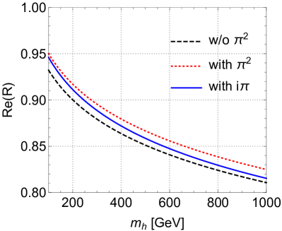
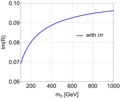
Figure 2: The ratio $R$ of the resummed result over the leading order result. Its real and imaginary part are shown on the left and right plot, respectively. The dashed black and dotted red line (on the left plot) denotes the result of Eq.(49) with $L^{2}$ replaced by $\ln^{2}(m_{h}^{2}/m_{b}^{2})$ and $\ln^{2}(m_{h}^{2}/m_{b}^{2})-\pi^{2}$, respectively. The blue line represents the result with $L^{2}=\ln^{2}(m_{h}^{2}/m_{b}^{2})-\pi^{2}-2i\pi\ln(m_{h}^{2}/m_{b}^{2})$. We have used $\alpha_{s}(m_{h})=0.113,m_{b}=5$ GeV.

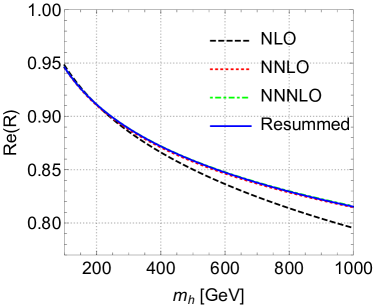
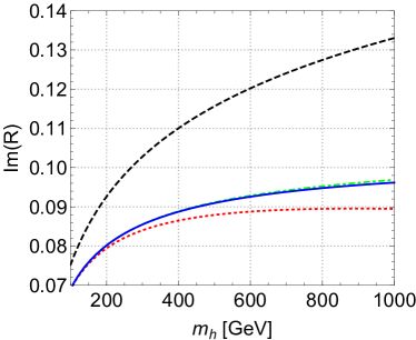
Figure 3: Same as Fig. 2 with $L^{2}=\ln^{2}(m_{h}^{2}/m_{b}^{2})-\pi^{2}-2i\pi\ln(m_{h}^{2}/m_{b}^{2})$ but with more lines to show the expanded results. Notice that the legends NLO, NNLO, NNNLO do not denote the full fixed-order results, but only the leading logarithms.

5 Conclusions

We have provided a method to resum the large logarithms in loop-induced processes with soft-collinear effective theory. This method is different from the conventional threshold or transverse momentum resummation, because the leading-order contributions have already divergences in the soft and collinear limits. By adopting a $\Delta$-regulator and a cut-off renormalization for the quark loop transverse momentum, we can make the leading-order result finite. Further, there are several sectors in the effective field theory contributing to the leading power expansion of the QCD amplitude. Each of them depends on the rapidity regulators. In particular, the contributions from (anti-)collinear sectors are proportional to $\ln(\Delta_{1,2}/m_{h}^{2})$ so that we can choose a special value of the regulator to make them vanishing. Then one only needs to consider the contribution from the soft sector, which has a structure ready to be resummed. Expanding the resummed result to the first two orders, we find agreement with previous QCD calculations. Compared with the resummation method using off-shell Sudakov form factor, we reproduce the full double logarithms $\ln^{2}(-m_{h}^{2}/m_{b}^{2}-i0)$. As a consequence, the large $\pi^{2}$ terms and the leading contribution of the imaginary part of the amplitude can also be resummed. In future, it would be interesting to explore the resummation beyond leading logarithmic accuracy. It is also promising to extend our scheme to more general cases, such as processes with non-Abelian gauge bosons or processes with more external particles, which are more important for collider phenomenology.

Appendix A Cancellation of the divergences at the two-loop level

We have claimed in the main text that the divergences in the first line of Eq.(32) cancel. Here we present the explicit results at two loop. Since the divergences will appear after integrating $p_{T}>m_{h}$, we must keep the $(p_{T}^{2}+m_{b}^{2})^{-\epsilon}$ at higher orders. Firstly, in the collinear sector, the higher-order hard and collider corrections are given by

$$B_{H} =-\frac{\alpha_{s}C_{F}}{2\pi}\frac{1}{\epsilon^{2}}\bigg{[}\bigg{(}\frac{-m_{h}^{2}}{\mu^{2}}\bigg{)}^{-\epsilon}-\bigg{(}\frac{-m_{h}^{2}z}{\mu^{2}}\bigg{)}^{-\epsilon}\bigg{]},$$ (50)

$$B_{C} =-\frac{\alpha_{s}C_{F}}{2\pi}\frac{1}{\epsilon^{2}}\bigg{[}\bigg{(}\frac{m_{T}^{2}}{\mu^{2}}\bigg{)}^{-\epsilon}-\bigg{(}\frac{m_{T}^{2}}{z\mu^{2}}\bigg{)}^{-\epsilon}\bigg{]}$$ (51)

with $m_{T}^{2}\equiv p_{T}^{2}+m_{b}^{2}$. If we expand the above result in $\epsilon$, we obtain the $O(\alpha_{s})$ part in Sec.3. Here we prefer to keep the full $\epsilon$ dependence because all the power series of $\epsilon$ will contribute to the divergence after integration. We have kept the $p_{T}$ dependence in $B_{C}$ in order to see that the cancellation of $\Delta$ regulators and divergences among the (anti-)collinear and soft sectors more clearly. It is ready to perform the integration,

$$\mu^{2\epsilon}\int_{m_{h}^{2}}^{\infty}dm_{T}^{2}(m_{T}^{2})^{-1-\epsilon}\int_{0}^{1}dz\frac{1}{z+\delta_{2}}(B_{H}+B_{C})=\mu^{2\epsilon}\int_{m_{h}^{2}}^{\infty}dm_{T}^{2}(m_{T}^{2})^{-1-\epsilon}$$

$$\frac{\alpha_{s}C_{F}}{2\pi}\frac{1}{\epsilon^{2}}\left[\left(\frac{-m_{h}^{2}}{\mu^{2}}\right)^{-\epsilon}\left(-\frac{1}{\epsilon}(1-\delta_{2}^{-\epsilon})+\ln\delta_{2}\right)+\left(\frac{m_{T}^{2}}{\mu^{2}}\right)^{-\epsilon}\left(\frac{1}{\epsilon}(1-\delta_{2}^{\epsilon})+\ln\delta_{2}\right)\right]$$

$$= \frac{\alpha_{s}C_{F}}{2\pi}\left(\frac{1}{4\epsilon^{2}}\ln^{2}\delta_{2}-\frac{1}{4\epsilon}\ln^{3}\delta_{2}\right)+O(\epsilon^{0})$$ (52)

with $\delta_{2}\equiv\Delta_{2}/m_{h}^{2}$. As before, we only keep the leading logarithms in the calculation. The anti-collinear result is obtained by changing $\delta_{2}\to\delta_{1}\equiv\Delta_{1}/m_{h}^{2}$.

Then we turn to the soft sector. The higher-order hard, (anti-)collinear and soft corrections are given by

$$D_{H} =-\frac{\alpha_{s}C_{F}}{2\pi}\frac{1}{\epsilon^{2}}\bigg{(}\frac{-m_{h}^{2}}{\mu^{2}}\bigg{)}^{-\epsilon},$$ (53)

$$D_{C} =\frac{\alpha_{s}C_{F}}{2\pi}\frac{1}{\epsilon^{2}}\bigg{(}\frac{m_{T}^{2}}{z\mu^{2}}\bigg{)}^{-\epsilon},$$ (54)

$$D_{\bar{C}} =\frac{\alpha_{s}C_{F}}{2\pi}\frac{1}{\epsilon^{2}}\bigg{(}\frac{-m_{h}^{2}z}{\mu^{2}}\bigg{)}^{-\epsilon},$$ (55)

$$D_{S} =-\frac{\alpha_{s}C_{F}}{2\pi}\frac{1}{\epsilon^{2}}\bigg{(}\frac{m_{T}^{2}}{\mu^{2}}\bigg{)}^{-\epsilon}.$$ (56)

We see that their sum $D_{t}\equiv D_{H}+D_{C}+D_{\bar{C}}+D_{S}$ is the same as the collinear sector $B_{H}+B_{C}$. We divide the integration of $z$ into two parts,

$$\mu^{2\epsilon}\int_{m_{h}^{2}}^{\infty}dm_{T}^{2}(m_{T}^{2})^{-\epsilon}\bigg{(}\int_{0}^{1}dz+\int_{1}^{\infty}dz\bigg{)}\frac{D_{t}}{z+\delta_{2}}\frac{1}{m_{T}^{2}-z\Delta_{1}}.$$ (57)

In the first part, we can drop the $\Delta_{1}$ regulator since $z$ is finite in this case. In the second part, we can drop the $\delta_{2}$ regulator since $z$ is larger than 1. As a consequence, the first part after integration will give the same result as Eq.(52). The second part is given by

$$\mu^{2\epsilon}\int_{m_{h}^{2}}^{\infty}dm_{T}^{2}(m_{T}^{2})^{-1-\epsilon}\frac{\alpha_{s}C_{F}}{2\pi}\frac{1}{\epsilon^{2}}\Bigg{\{}\left(\frac{-m_{h}^{2}}{\mu^{2}}\right)^{-\epsilon}\left[\frac{1}{\epsilon}\left(1-\left(\frac{-\Delta_{1}}{m_{T}^{2}}\right)^{\epsilon}\right)+\ln\frac{-\Delta_{1}}{m_{T}^{2}}\right]$$

$$\hskip 128.0374pt+\left(\frac{m_{T}^{2}}{\mu^{2}}\right)^{-\epsilon}\left[-\frac{1}{\epsilon}\left(1-\left(\frac{-\Delta_{1}}{m_{T}^{2}}\right)^{-\epsilon}\right)+\ln\frac{-\Delta_{1}}{m_{T}^{2}}\right]\Bigg{\}}$$

$$= \frac{\alpha_{s}C_{F}}{2\pi}\left(\frac{-m_{h}^{2}}{\mu^{2}}\right)^{-2\epsilon}\bigg{(}\frac{-1}{4\epsilon^{4}}+\frac{1}{4\epsilon^{2}}\ln^{2}\delta_{1}-\frac{1}{4\epsilon}\ln^{3}\delta_{1}\bigg{)}+O(\epsilon^{0}).$$ (58)

The $\delta_{1}$ dependent part has the same form as Eq.(52).

Lastly, the hard sector is given by

$$\frac{\alpha_{s}C_{F}}{2\pi}\left(\frac{-m_{h}^{2}}{\mu^{2}}\right)^{-2\epsilon}\frac{-1}{4\epsilon^{4}}.$$ (59)

And we see immediately that the divergences in

$$\mathcal{A}_{H}\left(\epsilon\right)+\left[\mathcal{A}_{C}\left(\epsilon,\Delta_{2}\right)\right]_{p_{T}>m_{h}}+\left[\mathcal{A}_{\bar{C}}\left(\epsilon,\Delta_{1}\right)\right]_{p_{T}>m_{h}}-\left[\mathcal{A}_{S}\left(\epsilon,\Delta_{1},\Delta_{2}\right)\right]_{p_{T}>m_{h}}$$ (60)

cancel each other. Moreover, based on the above results, one can also find that the $\Delta$ dependences in $\mathcal{A}_{C}+\mathcal{A}_{\bar{C}}-\mathcal{A}_{S}$ cancel for each fixed $p_{T}$.

References

• [1] G. F. Sterman, Summation of Large Corrections to Short Distance Hadronic Cross-Sections, Nucl. Phys. B281 (1987) 310.
• [2] S. Catani and L. Trentadue, Resummation of the QCD Perturbative Series for Hard Processes, Nucl. Phys. B327 (1989) 323.
• [3] G. P. Korchemsky and G. Marchesini, Resummation of large infrared corrections using Wilson loops, Phys. Lett. B313 (1993) 433.
• [4] H. Contopanagos, E. Laenen and G. F. Sterman, Sudakov factorization and resummation, Nucl. Phys. B484 (1997) 303 [hep-ph/9604313].
• [5] S. Forte and G. Ridolfi, Renormalization group approach to soft gluon resummation, Nucl. Phys. B650 (2003) 229 [hep-ph/0209154].
• [6] A. Banfi, G. P. Salam and G. Zanderighi, Principles of general final-state resummation and automated implementation, JHEP 03 (2005) 073 [hep-ph/0407286].
• [7] T. Becher and M. Neubert, Threshold resummation in momentum space from effective field theory, Phys. Rev. Lett. 97 (2006) 082001 [hep-ph/0605050].
• [8] G. Luisoni and S. Marzani, QCD resummation for hadronic final states, J. Phys. G42 (2015) 103101 [1505.04084].
• [9] D. Bonocore, E. Laenen, L. Magnea, L. Vernazza and C. D. White, The method of regions and next-to-soft corrections in Drell–Yan production, Phys. Lett. B742 (2015) 375 [1410.6406].
• [10] D. Bonocore, E. Laenen, L. Magnea, S. Melville, L. Vernazza and C. D. White, A factorization approach to next-to-leading-power threshold logarithms, JHEP 06 (2015) 008 [1503.05156].
• [11] D. Bonocore, E. Laenen, L. Magnea, L. Vernazza and C. D. White, Non-abelian factorisation for next-to-leading-power threshold logarithms, JHEP 12 (2016) 121 [1610.06842].
• [12] V. Del Duca, E. Laenen, L. Magnea, L. Vernazza and C. D. White, Universality of next-to-leading power threshold effects for colourless final states in hadronic collisions, JHEP 11 (2017) 057 [1706.04018].
• [13] N. Bahjat-Abbas, J. Sinninghe Damsté, L. Vernazza and C. D. White, On next-to-leading power threshold corrections in Drell-Yan production at N3LO, JHEP 10 (2018) 144 [1807.09246].
• [14] A. Bhattacharya, I. Moult, I. W. Stewart and G. Vita, Helicity Methods for High Multiplicity Subleading Soft and Collinear Limits, JHEP 05 (2019) 192 [1812.06950].
• [15] M. van Beekveld, W. Beenakker, E. Laenen and C. D. White, Next-to-leading power threshold effects for inclusive and exclusive processes with final state jets, 1905.08741.
• [16] M. van Beekveld, W. Beenakker, R. Basu, E. Laenen, A. Misra and P. Motylinski, Next-to-leading power threshold effects for resummed prompt photon production, 1905.11771.
• [17] R. Boughezal, A. Isgrò and F. Petriello, Next-to-leading power corrections to $V+1$ jet production in $N$-jettiness subtraction, 1907.12213.
• [18] I. Moult, L. Rothen, I. W. Stewart, F. J. Tackmann and H. X. Zhu, Subleading Power Corrections for N-Jettiness Subtractions, Phys. Rev. D95 (2017) 074023 [1612.00450].
• [19] R. Boughezal, X. Liu and F. Petriello, Power Corrections in the N-jettiness Subtraction Scheme, JHEP 03 (2017) 160 [1612.02911].
• [20] I. Moult, L. Rothen, I. W. Stewart, F. J. Tackmann and H. X. Zhu, N -jettiness subtractions for $gg\to H$ at subleading power, Phys. Rev. D97 (2018) 014013 [1710.03227].
• [21] R. Boughezal, A. Isgrò and F. Petriello, Next-to-leading-logarithmic power corrections for $N$-jettiness subtraction in color-singlet production, Phys. Rev. D97 (2018) 076006 [1802.00456].
• [22] M. A. Ebert, I. Moult, I. W. Stewart, F. J. Tackmann, G. Vita and H. X. Zhu, Power Corrections for N-Jettiness Subtractions at ${\cal O}(\alpha_{s})$, JHEP 12 (2018) 084 [1807.10764].
• [23] I. Balitsky and A. Tarasov, Higher-twist corrections to gluon TMD factorization, JHEP 07 (2017) 095 [1706.01415].
• [24] I. Balitsky and A. Tarasov, Power corrections to TMD factorization for Z-boson production, JHEP 05 (2018) 150 [1712.09389].
• [25] M. A. Ebert, I. Moult, I. W. Stewart, F. J. Tackmann, G. Vita and H. X. Zhu, Subleading power rapidity divergences and power corrections for qT, JHEP 04 (2019) 123 [1812.08189].
• [26] L. Cieri, C. Oleari and M. Rocco, Higher-order power corrections in a transverse-momentum cut for colour-singlet production at NLO, Eur. Phys. J. C79 (2019) 852 [1906.09044].
• [27] R. J. Hill, T. Becher, S. J. Lee and M. Neubert, Sudakov resummation for subleading SCET currents and heavy-to-light form-factors, JHEP 07 (2004) 081 [hep-ph/0404217].
• [28] M. Beneke and D. Yang, Heavy-to-light B meson form-factors at large recoil energy: Spectator-scattering corrections, Nucl. Phys. B736 (2006) 34 [hep-ph/0508250].
• [29] S. M. Freedman and R. Goerke, Renormalization of Subleading Dijet Operators in Soft-Collinear Effective Theory, Phys. Rev. D90 (2014) 114010 [1408.6240].
• [30] R. Goerke and M. Inglis-Whalen, Renormalization of dijet operators at order 1/Q2 in soft-collinear effective theory, JHEP 05 (2018) 023 [1711.09147].
• [31] M. Beneke, M. Garny, R. Szafron and J. Wang, Anomalous dimension of subleading-power N-jet operators, JHEP 03 (2018) 001 [1712.04416].
• [32] M. Beneke, M. Garny, R. Szafron and J. Wang, Anomalous dimension of subleading-power $N$-jet operators. Part II, JHEP 11 (2018) 112 [1808.04742].
• [33] M. Beneke, M. Garny, R. Szafron and J. Wang, Violation of the Kluberg-Stern-Zuber theorem in SCET, JHEP 09 (2019) 101 [1907.05463].
• [34] I. Moult, I. W. Stewart, G. Vita and H. X. Zhu, First Subleading Power Resummation for Event Shapes, JHEP 08 (2018) 013 [1804.04665].
• [35] I. Moult, I. W. Stewart and G. Vita, Subleading Power Factorization with Radiative Functions, JHEP 11 (2019) 153 [1905.07411].
• [36] I. Moult, I. W. Stewart, G. Vita and H. X. Zhu, The Soft Quark Sudakov, 1910.14038.
• [37] M. Beneke, A. Broggio, M. Garny, S. Jaskiewicz, R. Szafron, L. Vernazza et al., Leading-logarithmic threshold resummation of the Drell-Yan process at next-to-leading power, JHEP 03 (2019) 043 [1809.10631].
• [38] N. Bahjat-Abbas, D. Bonocore, J. Sinninghe Damsté, E. Laenen, L. Magnea, L. Vernazza et al., Diagrammatic resummation of leading-logarithmic threshold effects at next-to-leading power, 1905.13710.
• [39] M. Beneke, M. Garny, S. Jaskiewicz, R. Szafron, L. Vernazza and J. Wang, Leading-logarithmic threshold resummation of Higgs production in gluon fusion at next-to-leading power, 1910.12685.
• [40] M. Beneke, A. Broggio, S. Jaskiewicz and L. Vernazza, Threshold factorization of the Drell-Yan process at next-to-leading power, 1912.01585.
• [41] I. Moult, G. Vita and K. Yan, Subleading Power Resummation of Rapidity Logarithms: The Energy-Energy Correlator in $\mathcal{N}=4$ SYM, 1912.02188.
• [42] G. Jikia and A. Tkabladze, QCD corrections to heavy quark pair production in polarized gamma gamma collisions and the intermediate mass Higgs signal, Phys. Rev. D54 (1996) 2030 [hep-ph/9601384].
• [43] V. S. Fadin, V. A. Khoze and A. D. Martin, Higgs studies in polarized gamma gamma collisions, Phys. Rev. D56 (1997) 484 [hep-ph/9703402].
• [44] M. I. Kotsky and O. I. Yakovlev, On the resummation of double logarithms in the process Higgs $\to$ gamma gamma, Phys. Lett. B418 (1998) 335 [hep-ph/9708485].
• [45] R. Akhoury, H. Wang and O. I. Yakovlev, On the Resummation of large QCD logarithms in Higgs $\to$ gamma gamma decay, Phys. Rev. D64 (2001) 113008 [hep-ph/0102105].
• [46] K. Melnikov and A. Penin, On the light quark mass effects in Higgs boson production in gluon fusion, JHEP 05 (2016) 172 [1602.09020].
• [47] E. Braaten, H. Zhang and J.-W. Zhang, Mass Dependence of Higgs Production at Large Transverse Momentum, JHEP 11 (2017) 127 [1704.06620].
• [48] E. Braaten, H. Zhang and J.-W. Zhang, Mass dependence of Higgs boson production at large transverse momentum through a bottom-quark loop, Phys. Rev. D97 (2018) 096014 [1707.09857].
• [49] A. A. Penin, High-Energy Limit of Quantum Electrodynamics beyond Sudakov Approximation, Phys. Lett. B745 (2015) 69 [1412.0671].
• [50] A. A. Penin and N. Zerf, Two-loop Bhabha Scattering at High Energy beyond Leading Power Approximation, Phys. Lett. B760 (2016) 816 [1606.06344].
• [51] T. Liu and A. A. Penin, High-Energy Limit of QCD beyond the Sudakov Approximation, Phys. Rev. Lett. 119 (2017) 262001 [1709.01092].
• [52] S. Alte, M. König and M. Neubert, Effective Field Theory after a New-Physics Discovery, JHEP 08 (2018) 095 [1806.01278].
• [53] T. Liu and A. Penin, High-Energy Limit of Mass-Suppressed Amplitudes in Gauge Theories, JHEP 11 (2018) 158 [1809.04950].
• [54] S. Alte, M. König and M. Neubert, Effective Theory for a Heavy Scalar Coupled to the SM via Vector-Like Quarks, Eur. Phys. J. C79 (2019) 352 [1902.04593].
• [55] M. Inoue, R. Najima, T. Oka and J. Saito, QCD corrections to two photon decay of the Higgs boson and its reverse process, Mod. Phys. Lett. A9 (1994) 1189.
• [56] M. Spira, A. Djouadi, D. Graudenz and P. M. Zerwas, Higgs boson production at the LHC, Nucl. Phys. B453 (1995) 17 [hep-ph/9504378].
• [57] J. Fleischer, O. V. Tarasov and V. O. Tarasov, Analytical result for the two loop QCD correction to the decay H $\to$ 2 gamma, Phys. Lett. B584 (2004) 294 [hep-ph/0401090].
• [58] R. Harlander and P. Kant, Higgs production and decay: Analytic results at next-to-leading order QCD, JHEP 12 (2005) 015 [hep-ph/0509189].
• [59] C. Anastasiou, S. Beerli, S. Bucherer, A. Daleo and Z. Kunszt, Two-loop amplitudes and master integrals for the production of a Higgs boson via a massive quark and a scalar-quark loop, JHEP 01 (2007) 082 [hep-ph/0611236].
• [60] U. Aglietti, R. Bonciani, G. Degrassi and A. Vicini, Analytic Results for Virtual QCD Corrections to Higgs Production and Decay, JHEP 01 (2007) 021 [hep-ph/0611266].
• [61] M. Spira, Higgs Boson Production and Decay at Hadron Colliders, Prog. Part. Nucl. Phys. 95 (2017) 98 [1612.07651].
• [62] Z. L. Liu and M. Neubert, Factorization at Subleading Power and Endpoint-Divergent Convolutions in $h\to\gamma\gamma$ Decay, 1912.08818.
• [63] V. A. Smirnov, Asymptotic expansions of two loop Feynman diagrams in the Sudakov limit, Phys. Lett. B404 (1997) 101 [hep-ph/9703357].
• [64] M. Beneke and V. A. Smirnov, Asymptotic expansion of Feynman integrals near threshold, Nucl. Phys. B522 (1998) 321 [hep-ph/9711391].
• [65] C. W. Bauer, S. Fleming and M. E. Luke, Summing Sudakov logarithms in B $\to$ $X_{s}$ + gamma in effective field theory, Phys. Rev. D63 (2000) 014006 [hep-ph/0005275].
• [66] C. W. Bauer, S. Fleming, D. Pirjol and I. W. Stewart, An Effective field theory for collinear and soft gluons: Heavy to light decays, Phys.Rev. D63 (2001) 114020 [hep-ph/0011336].
• [67] C. W. Bauer, D. Pirjol and I. W. Stewart, Soft collinear factorization in effective field theory, Phys.Rev. D65 (2002) 054022 [hep-ph/0109045].
• [68] C. W. Bauer, S. Fleming, D. Pirjol, I. Z. Rothstein and I. W. Stewart, Hard scattering factorization from effective field theory, Phys. Rev. D66 (2002) 014017 [hep-ph/0202088].
• [69] M. Beneke, A. Chapovsky, M. Diehl and T. Feldmann, Soft collinear effective theory and heavy to light currents beyond leading power, Nucl.Phys. B643 (2002) 431 [hep-ph/0206152].
• [70] A. K. Leibovich, Z. Ligeti and M. B. Wise, Comment on quark masses in SCET, Phys. Lett. B564 (2003) 231 [hep-ph/0303099].
• [71] J. Chay, C. Kim, Y. G. Kim and J.-P. Lee, Soft Wilson lines in soft-collinear effective theory, Phys. Rev. D71 (2005) 056001 [hep-ph/0412110].
• [72] A. V. Manohar and I. W. Stewart, The Zero-Bin and Mode Factorization in Quantum Field Theory, Phys. Rev. D76 (2007) 074002 [hep-ph/0605001].
• [73] A. Idilbi and T. Mehen, On the equivalence of soft and zero-bin subtractions, Phys. Rev. D75 (2007) 114017 [hep-ph/0702022].
• [74] A. Idilbi and T. Mehen, Demonstration of the equivalence of soft and zero-bin subtractions, Phys. Rev. D76 (2007) 094015 [0707.1101].
• [75] J.-y. Chiu, A. Fuhrer, A. H. Hoang, R. Kelley and A. V. Manohar, Soft-Collinear Factorization and Zero-Bin Subtractions, Phys. Rev. D79 (2009) 053007 [0901.1332].
• [76] T. Becher and G. Bell, Analytic regularization in Soft-Collinear Effective Theory, Phys. Lett. B713 (2012) 41 [1112.3907].
• [77] T. Becher and M. Neubert, On the Structure of Infrared Singularities of Gauge-Theory Amplitudes, JHEP 06 (2009) 081 [0903.1126].
• [78] M. Neubert, Renormalization-group improved calculation of the B $\to$ $X_{s}$ gamma branching ratio, Eur. Phys. J. C40 (2005) 165 [hep-ph/0408179].