Gravitational-Wave Constraints on an Effective–Field-Theory Extension of General Relativity

Abstract

Gravitational-wave observations of coalescing binary systems allow for novel tests of the strong-field regime of gravity. Using data from the Gravitational Wave Open Science Center (GWOSC) of the LIGO and Virgo detectors, we place the first constraints on an effective–field-theory based extension of General Relativity in which only higher-order curvature terms are added to the Einstein-Hilbert action. We construct gravitational-wave templates describing the quasi-circular, adiabatic inspiral phase of binary black holes in this extended theory of gravity. Then, after explaining how to properly take into account the region of validity of the effective field theory when performing tests of General Relativity, we perform Bayesian model selection using the two lowest-mass binary–black-hole events reported to date by LIGO and Virgo —GW151226 and GW170608— and constrain this theory with respect to General Relativity. We find that these data disfavors the appearance of new physics on distance scales around $\sim 150$ km. Finally, we describe a general strategy for improving constraints as more observations will become available with future detectors on the ground and in space.

I Introduction

The detections of gravitational waves (GWs) from merging black-hole (BH) and neutron-star binaries by the LIGO and Virgo collaborations Abbott et al. (2019a) provide a novel opportunity to test the highly-dynamical, strong-field regime of gravity. All tests to date indicate that these observations are fully consistent with the predictions of General Relativity (GR) Abbott et al. (2016a); Yunes et al. (2016); Abbott et al. (2018, 2019b). Combined with tests from the Solar System and cosmological observations Will (2014); Baker et al. (2015, 2019), we now have a great amount of evidence that GR accurately describes gravity over a broad range of scales.

While positive checks for consistency are significant results by themselves, it remains important also to consider how GW observations can directly inform our understanding of how gravity behaves in the high-curvature regime. Work towards this second goal typically proceeds in one of two directions. One option is to consider a particular alternative to GR (typically at the level of an action), then calculate how the differences in the underlying physical theory translate to an observable signal, i.e., the gravitational waveform, and finally use a detected GW to measure the physical parameters that define that theory. While straightforward, this approach suffers due to its specificity; a plethora of proposals for modifying GR in the high-curvature regime have been considered Berti et al. (2015), and testing each individually is highly inefficient. The second option instead considers phenomenological deviations Arun et al. (2006); Yunes and Pretorius (2009); Mishra et al. (2010); Li et al. (2012); Agathos et al. (2014) from the expected GW signal in GR, it uses observations to constrain these deviations, and then maps those bounds to constraints on specific non-GR theories Yunes et al. (2016); Nair et al. (2019). But, this approach does not always provide a clear connection to the fundamental physics/principles one wishes to test.

In this work, we adopt an alternative approach, employing the powerful tools of Effective Field Theory (EFT) to test natural extensions of GR with GW observations. Broadly speaking, EFT provides a systematic framework to encode all modifications to an existing theory that could arise after introducing some form of new physics. Though this task may seem daunting, the construction of an EFT is dramatically simplified by restricting ourselves to modifications that: (i) respect certain general principles or symmetries (e.g., locality and Lorentz invariance), and (ii) are associated with a particle (or some form of undetermined excitation) whose mass is too large to be directly probed with experiments. Under these assumptions, the Lagrangian of our EFT is determined by simply adding to the original Lagrangian all possible terms allowed by the symmetries that we wish to preserve, constructed using the fields already present in the original theory. Dimensional analysis dictates that these new terms are each suppressed by some energy scale, dubbed collectively as the cutoff scale $\Lambda_{c}$, which, roughly speaking, corresponds to the mass of the particles that modify the original theory. Note that describing physics at energies above this cutoff would require the introduction of new particles to the theory, or equivalently, new fields to the effective Lagrangian, vastly complicating the problem. However, provided we work at energies below the cutoff scale [assumption (ii) above], all physical observables can be estimated without specifying these new particles in detail. The high-energy-agnosticism of the EFT provides the primary advantage of this approach over the tests of specific alternative theories described earlier; by working within the confines of an EFT, we can simultaneously test a large range of possible extensions of GR at once.

Reference Endlich et al. (2017) constructed an EFT suitable for testing gravity with current GW experiments following the guidelines above. In this paper, we examine the constraints that can be set on this extension of GR given existing GW observations. The work is organized as follows. In Sec. II, we review the main properties of the EFT extension of GR constructed in Ref. Endlich et al. (2017). In Sec. III we construct gravitational waveforms that describe the quasi-circular, adiabatic inspiral of BBHs in this theory. Then, in Sec. IV, we employ Bayesian inference, notably the model-selection method, to place constraints on this theory when $\Lambda_{c}\lesssim 1/r_{s}$, $r_{s}$ being the BH radius, demonstrating that current GW data rule out modifications to GR entering at scales around $\Lambda_{c}^{-1}\sim 150$ km (or equivalently, $\Lambda_{c}\sim 1.3$ peV). Finally, we provide some concluding remarks and discuss future directions in Sec. V. Lastly, in the Appendix A, we consider setting constraints in the regime $\Lambda_{c}\gtrsim 1/r_{s}$, while in the Appendix B we discuss how our findings are modified if an inspiral-merger-ringdown waveform model instead of an inspiral-only model were used. Henceforth, we use natural units $G=c=1$ except when stated otherwise.

II Effective–field-theory extension of General Relativity

II.1 Extension of General Relativity using high powers in Riemann tensor

The EFT constructed in Ref. Endlich et al. (2017) encodes the most general extension to gravity under a number of assumptions: (i) the following principles and symmetries are preserved by the new physics: locality, causality, Lorentz invariance, unitarity and diffeomorphism invariance, (ii) there is no new particle lighter than the cutoff of the theory, and (iii) the extension to the theory is testable with experiments such as LIGO and Virgo. The resulting EFT takes the form

$$S_{\rm eff}=2M_{\rm pl}^{2}\int d^{4}x\sqrt{-g}\left(-R+\frac{\mathcal{C}^{2}}{\Lambda^{6}}+\frac{\tilde{\mathcal{C}}^{2}}{\tilde{\Lambda}^{6}}+\frac{\mathcal{C}\,\tilde{\mathcal{C}}}{\Lambda_{-}^{6}}\right)+\ldots\,,$$ (1)

where $M_{\text{pl}}=\sqrt{\hbar}$ is the Planck mass,

$$\mathcal{C}\equiv R_{\alpha\beta\gamma\delta}\,R^{\alpha\beta\gamma\delta}\,,\quad\tilde{\mathcal{C}}\equiv R_{\alpha\beta\gamma\delta}\,\epsilon^{\alpha\beta\phantom{\mu}\phantom{\nu}}_{\phantom{\alpha}\phantom{\beta}\mu\nu}\,R^{\mu\nu\gamma\delta}\,,$$ (2)

where $\Lambda,\tilde{\Lambda},\Lambda_{-}$ are cutoff scales for each operator, and the dots in Eq. (1) denote terms with powers in the Riemann tensor beyond four. Though the cutoff scale for each term is, in principle, independent, it is quite natural to assume that they are comparable (i.e., $\Lambda\sim\tilde{\Lambda}\sim\Lambda_{-}$.) In Eq. (2), we employ the Levi-Civita tensor $\epsilon^{\mu\nu\rho\sigma}$, defined such that $\epsilon^{0123}=1/\sqrt{-g}$. We refer to the EFT (1) as “EFT of General Relativity”, in short EFTGR. Except where noted, we assume the coupling constants to be positive (i.e., $\Lambda^{6},\tilde{\Lambda}^{6},\Lambda_{-}^{6}>0$), however, in principle one should not dismiss the parameter space $\Lambda^{6},\tilde{\Lambda}^{6},\Lambda_{-}^{6}<0$ Endlich et al. (2017) .

It is well known that the terms in Eq. (1), as well as others, are needed by the renormalizability of the theory (e.g., see Ref. Goroff and Sagnotti (1986)). Renormalizability, however, suggests that the scales suppressing those operators are different from the ones in Eq. (1). In fact, the main novelty of Eq. (1) lies in realizing that such low-energy suppression for those operators and such scalings were possible from an EFT point of view, and, as we will describe, are not yet ruled out by tests of gravity. The label of EFTGR is referred in this paper only to the particular scaling assumed in Eq. (1), which gives a theory testable by LIGO and Virgo, and not to the general, and already well-established fact, that GR is an EFT (e.g., see Ref. Endlich et al. (2017) for detailed discussions).

For clarity, we now briefly review the construction of the action (1); the interested reader should refer to Ref. Endlich et al. (2017) for more detail. As discussed above, our assumption that no new particle enters with a mass below the cutoff of the EFT precludes the introduction of any new fields to the theory; thus our effective action must only be a function of the metric $g_{\mu\nu}$. Furthermore, our assumption of diffeomorphism invariance implies that new terms must be expressible as functions of the Riemann tensor and its covariant derivatives. Consider a Taylor expansion of such a function: dimensional analysis dictates that terms polynomial in the Riemann tensor must be suppressed by powers of some cutoff scale $\Lambda_{c}$. In principle, we could write an infinite number of higher-order curvature terms suppressed by correspondingly large powers of some cutoff scale [i.e., terms given schematically by $(R_{\mu\nu\rho\sigma}/\Lambda_{c}^{2})^{n}$]. But, if we are interested in observables whose energy scale $E$ is much smaller than $\Lambda_{c}$ (as in the present context), then each term, schematically of the form $(R_{\mu\nu\rho\sigma}/\Lambda^{2})^{n}$, contributes as $(E^{2}/\Lambda^{2})^{n}\ll 1$. Therefore, for a given precision of the prediction, only a finite number of terms needs to be kept.

For our purposes, we keep only the leading-order corrections to the Einstein-Hilbert action; these are precisely the terms given in Eq. (1). However, our truncation of the higher-order curvature corrections remains valid only so long as the sub-dominant terms remain negligible at the level of precision at which we work. Yet, working within this restricted regime of validity, we see that any extension of GR that upholds conditions (i) and (ii) described above must admit a low-energy  EFT of the form (1).

Note that the leading-order corrections to the Einstein-Hilbert Lagrangian come from terms that are quartic in the Riemann tensor (or equivalently, eight derivatives of the metric) rather than terms quadratic or cubic in curvature. In vacuum (to which we restrict our attention), terms quadratic in the Riemann tensor can be removed via an appropriate redefinition of the gravitational field . Our dismissal of terms cubic in Riemann is more subtle. There are several theoretical arguments that disfavor the presence of these terms, see Refs. Camanho et al. (2016); Reall and Santos (2019), as well as Sec. 2.2 of Ref. Endlich et al. (2017). Additionally, there are several cancellations in the post-Newtonian (PN) calculation of the contribution of these terms to the GW signal Endlich et al. (2017). This leads to the suppression of these effects, going as $v^{4}$ instead of $v^{2}$, as instead expected from naive estimates, and makes the computation of the non-vanishing effects a harder task due to proliferation of Feynman diagrams, as typically occurs once one goes beyond the leading order. In spite of these facts, further study of these terms remains an interesting direction that we leave for future work.

Finally, one can, in principle, include in the action (1) additional terms containing covariant derivatives of the Riemann tensor that equate to eight derivatives of the metric; however, these terms can always be absorbed into the existing terms in Eq. (1) via integration by parts (see Sec. 2.1 of Ref. Endlich et al. (2017)), and so we can work with the simplified action without any loss of generality.

Clearly, the higher-order curvature terms in Eq. (1) produce the greatest deviation from GR when the energy scales in the problem approach the cutoff scale of the EFT. In the context of a BBH system, this occurs when the cutoff scale is comparable to the inverse Schwarzschild radius of the merging BHs (the shortest curvature scale in the problem). For typical stellar-mass BHs observable by the LIGO and Virgo detectors, this corresponds to an energy scale of the order of inverse kilometers (or tens of picoelectron volts).

By particle physics standards, this energy cutoff is quite low. Indeed, there is no a priori expectation that GR should receive corrections at such low-energy scales. Yet, there remain several factors that merit further exploration of this EFT despite its contrivance. First, as we will discuss in more detail below, under some mild assumptions on the ultraviolet (UV) completion of this EFT, there is no experimental evidence that gravity excludes the possibility of new physics on the scale of inverse kilometers. Second, a presupposition of naturalness in our EFT is itself a theoretical bias; given the wealth of observational data now available from the LIGO and Virgo experiments, it is worthwhile to adopt a more agnostic viewpoint, letting the data determine the correct description of nature rather than our theoretical preconceptions. Finally, the Lagrangian in Eq. (1) with cutoff $\Lambda_{c}$ is consistent at classical and quantum level even for very low-energy cutoff $\Lambda_{c}$.

II.2 Soft ultraviolet completion of the effective–field-theory extension of General Relativity

The predictions of GR have been tested with exquisite precision in laboratory on the Earth and Solar-System experiments Will (2014). Naively, one may expect that such experiments could be sensitive to modifications of GR that enter at scales of inverse kilometers in the form of Eq. (1). However, there exist conditions under which the extensions of GR that we consider completely circumvent these weak-field constraints while still impacting strong-field phenomena detectable through GWs from stellar-mass BHs. In this subsection, we outline this additional condition precisely, which we denote as the existence of a soft ultraviolet (UV) completion.

The key distinction between the weak-field and strong-field regimes alluded to above is not the distance scales of the systems involved, but rather the curvature scales manifested in each. Typical curvature scales in the Solar System and terrestrial experiments are of the order of less than $10^{-8}\text{ km}^{-1}$ Baker et al. (2015), whereas stellar-mass BHs generate curvatures up to scales of inverse kilometers. Under the assumption of a soft UV completion, deviations from GR like those in Eq. (1) can still arise at cutoff scales $\Lambda_{c}$ of inverse kilometers, and yet have negligible effects on weak-field tests. A different point of contention may arise from tests of gravity that involve $X$-ray binaries Bambi (2014); Reynolds (2014); however, the precision of current observations is not high enough to rule out the models we consider here (see Sec. 8 of Ref. Endlich et al. (2017) for further discussion of all relevant experiments).

To outline what is meant by a soft UV completion, we first recall that the EFT in Eq. (1) breaks down at the scale $\Lambda_{c}$. Thus, to make predictions on shorter distances scales, one needs to introduce new degrees of freedom and use a more fundamental theory. As a result, one cannot guarantee that an EFT of the form (1) reduces to GR on distance scales shorter than $\Lambda_{c}^{-1}$. At energies (or inverse distances) below $\Lambda_{c}$, all EFT effects grow as $(E/\Lambda_{c})^{n}$ with $n>0$; if one extrapolates this growth to $E\gg\Lambda_{c}$, then the EFT effects grow very large at short distances. The assumption of a soft UV completion states exactly that this blow up at high energies does not occur. Namely, we assume that all EFT effects saturate at the EFT breakdown point $E\sim\Lambda_{c}$ and either stay constant or even decay at higher energies.

A similar sort of soft UV completion occurs in many familiar theories that have already been experimentally verified, most notably the Standard Model of particle physics. There, the scale $\Lambda_{c}$ is nothing but a mass of some heavy particle (e.g., the Higgs boson or the $W$-boson), $\Lambda_{c}\simeq m$. In these cases, at energies $E$ below the cutoff, the mass enters the predictions for many physical observables as $(E/m)^{n}$ with $n>0$; however, when $E>m$, the mass no longer enters in the denominator of any terms. Unfortunately, we are not able to provide any explicit example of a UV completion for our EFT (whether we require the softness assumption or not). But this fact only stresses the versatility of the EFT approach—we can make explicit predictions without the knowledge of the UV physics, which can be extremely complex. By working only within its regime of validity, we are able to place bounds on EFTGR with GW observations with no further assumption about the underlying short-distance theory besides that of a soft UV completion.

Let us mention that the soft UV completion assumption appears to be a very generic necessary requirement for extensions of GR to be potentially testable by GW observatories — for example there exist simple extensions of our EFT that differ by the addition of a single light scalar or pseudoscalar field which couples to the curvature invariant $\mathcal{C}$ or $\tilde{\mathcal{C}}$ correspondingly. These theories are usually called dynamical Gauss-Bonnet and dynamical Chern-Simons gravities in the literature (see, e.g., Ref. Berti et al. (2015)). Simple EFT analysis reveals that for the values of parameters testable by GW observatories these theories also must have a cutoff at the scale of order of the inverse Schwarzschild radius and require the same assumption about the short-distance behavior as our EFT Nair et al. (2019). These features, required by theoretical consistency, are often missed since these theories are not properly treated as EFTs (see, however, the recent works Okounkova et al. (2017); Witek et al. (2019); Okounkova et al. (2019a); Nair et al. (2019)). Possible infrared modifications of gravity, like theories of massive gravity, also require a similar sort of assumption about the UV completion  Vainshtein (1972).

II.3 Phenomenological consequences of the effective–field-theory extension of General Relativity

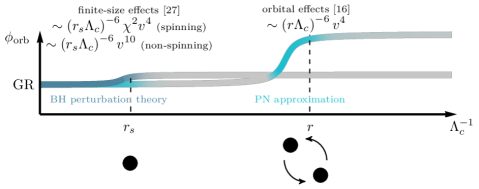
Figure 1: The phenomenological consequences of EFTGR in binary BH systems and the regimes of applicability of perturbative approximations in which they are computed. The vertical axis schematically depicts the corrections to a generic observable (here taken to be the orbital phase $\phi_{\text{orb}}$) relative to its prediction in GR as function of the inverse cutoff scale $\Lambda_{c}^{-1}$. For extensions to GR at distance scales below the Schwarzschild radii of the BHs $r_{s}$, one can use BH perturbation theory to compute the finite-size effects that influence the binary dynamics Cardoso et al. (2018), shown in dark blue. For $\Lambda_{c}^{-1}\gtrsim r_{s}$, this approximation scheme breaks down, shown in gray, and the finite-size effects cannot be computed explicitly; however, the assumption of a soft UV completion ensures that these effects saturate at $\Lambda_{c}\sim 1/r_{s}$, changing by no more than a factor of order one for cutoff energies below this value. Similarly, new orbital effects Endlich et al. (2017) are computed using the PN approximation; these corrections are subdominant to the aforementioned finite-size effects when the cutoff distance scale $\Lambda_{c}^{-1}$ is much smaller than the orbital separation $r$, but dominate when $\Lambda_{c}\sim 1/r$. However, by construction, EFTGR is only valid over distance scales larger than the $\Lambda_{c}^{-1}$, and so the PN prediction of new orbital effects cannot be extended to separations below $\Lambda_{c}^{-1}$. Thus, as shown in cyan, the PN approximation can be applied when $\Lambda_{c}^{-1}\lesssim r_{s}$, where both finite-size and orbital effects are known or when $\Lambda_{c}^{-1}\lesssim r$, where orbital effects are known and finite-size effects are small enough to be neglected.

There are several phenomenological consequences associated to the new terms present in Eq. (1). Let us focus on binaries comprised of two BHs of similar size, whose Schwarzschild radii we collectively denote with $r_{s}$. If $\Lambda_{c}\gtrsim 1/r_{s}$, the observable deviations from GR present in our EFT mainly arise from modifications to the Kerr geometry of each individual BH, as well as, the quasi-normal modes (QNMs) of the remnant BH produced by their merger. Reference Cardoso et al. (2018) investigated how the GR Kerr geometry is modified in this regime, showing that: i) the equatorial frequency at the light ring and innermost stable circular orbit (ISCO), and the spin-induced quadrupole moment receive corrections, ii) the $\mathbb{Z}_{2}$ symmetry of the geometry is broken, iii) the tidal Love numbers become non-vanishing, and iv) the QNM spectrum is modified with respect to GR even for non-spinning BHs. Various thermodynamical properties of BHs in this EFT were also recently studied in Ref. Reall and Santos (2019). We collectively refer to the corrections to binary dynamics and GW signal corresponding to these deformations of the Kerr geometry in EFTGR as finite-size effects; in Appendix A we show that these finite-size effects are too weak to be observable with current GW events, and therefore we are not yet able to put any constraints in the regime $\Lambda_{c}\gtrsim 1/r_{s}$.

Therefore in this paper we will instead focus on the opposite regime $\Lambda_{c}\lesssim 1/r_{s}$, whose phenomenological consequences were studied in Ref. Endlich et al. (2017) in larger detail (in particular, see Sec. 7 of Ref. Endlich et al. (2017) for the discussion of the two regimes). In this case, the EFT breaks down at distances larger than the gravitational radius and, due to the assumption of soft UV completion, the finite-size effects saturate , and the dominant signature of EFTGR in the GW signal arises from modifications of the two-body interactions between the BHs. As we will discuss in more detail below, these are corrections that enter at 2PN order, though they are additionally suppressed by a factor of $1/(\Lambda_{c}r)^{6}\ll 1$, with $r$ being the separation of the two BHs. Explicitly, the relative correction to the amplitude and phase of the GWs scales as $v^{4}/(\Lambda_{c}r)^{6}\sim v^{16}/(\Lambda_{c}r_{s})^{6}$, which can also be thought of as an 8PN term, albeit with an extraordinarily large coefficient. The relative size of finite-size effects and these new orbital effects—as well as the regimes of applicability of perturbative methods through which they are computed—are depicted schematically in Fig. 1; this figure also illustrates the saturation of corrections beyond the cutoff scale of our EFT, as imposed by the assumption of a soft UV completion.

In this regime (i.e., when $\Lambda_{c}\lesssim 1/r_{s}$), the corrections due to the modification to the intrinsic Kerr geometry cannot be computed explicitly, as this would require the full UV completion of the EFT. One can however estimate them at the level of order of magnitude. Finite-size effects from modifications to the spin-induced and tidally-induced quadrupole moments produce corrections to binary motion (and the subsequent GW signal) that scale as $\chi^{2}v^{4}$ and $v^{10}$, respectively, where $\chi$ is the dimensionless spin of the BHs. Note that we have used our assumption of a soft UV completion to eliminate the scaling with $\Lambda_{c}r_{s}$ in these terms; as detailed in the footnote above, we have assumed that these effects saturate for BHs of size $r_{s}\sim\Lambda_{c}^{-1}$, and thus this scaling can simply be replaced by an order one number in the regime we work $r_{s}\lesssim\Lambda_{c}^{-1}$. Using this simplification, we estimate the relative impact of these finite-size effects as compared to the orbital effects discussed above by computing the total number of GW cycles each contribute to the inspiral. For BHs of mass greater than $\sim 10M_{\odot}$, we find that the orbital effects typically contribute at least 100 times as many cycles as finite-size effects over the frequency bandwidth of the Advanced LIGO and Virgo detectors. Thus, we can safely neglect finite-size effects in our current study, leaving these details for future work.

III Gravitational-wave prediction for the inspiral regime in the effective–field-theory extension of General Relativity

In this section we explicitly show that because EFTGR modifies the conservative and dissipative dynamics of a two-body system, it leads to new terms in the GW phasing, which might be observed or constrained by GW observations.

In the early-inspiral phase the dynamics of a binary system of two objects with mass $m_{1}$ and $m_{2}$ can be characterized by an effective action that in center-of-mass frame takes the form Goldberger and Rothstein (2006); Endlich et al. (2017):

$$S=\int dt\left[m_{1}+m_{2}+\frac{1}{2}\mu\mathbf{v}^{2}(t)-V(r(t))+\frac{1}{2}Q_{ij}(t)R^{i0j0}+\ldots\right],$$ (3)

where $\mu=m_{1}m_{2}/(m_{1}+m_{2})$ is the reduced mass of the system, $\mathbf{v}(t)$ is the relative velocity between the objects, $V(r(t))$ is the potential energy, $Q_{ij}(t)$ is the mass quadrupole moment of the system and $\ldots$ denote higher-order multipole moments.

As shown in Ref. Endlich et al. (2017), in the PN and $\Lambda_{c}\lesssim 1/r_{s}$ regimes, the leading-order correction to the gravitational potential of a binary system with non-spinning or slowly-spinning components is generated by the term $\mathcal{C}^{2}$ in Eq. (1), and reads:

$$V_{\Lambda}=512\,\frac{m_{1}m_{2}}{r}\left(\frac{1}{\Lambda r}\right)^{6}\frac{(m_{1}^{2}+m_{2}^{2})}{r^{2}}\,.$$ (4)

The new terms in the action (1) also modify the gravitational radiation emitted by the binary. The leading order correction comes again from the term $\mathcal{C}^{2}$ Endlich et al. (2017), and it can be written as a renormalization of the Newtonian quadrupole-moment $Q^{\rm Newt}_{ij}$ of the binary system:

$$Q_{ij} = Q_{ij}^{\rm Newt}+\cdots+Q_{ij}^{\Lambda}\,,$$ (5)

$$Q^{\Lambda}_{ij} = 2688\,\left(\frac{1}{\Lambda r}\right)^{6}\left(\frac{m_{1}+m_{2}}{r}\right)^{2}\,Q^{\rm Newt}_{ij}\,,$$ (6)

where $\ldots$ denote higher order PN corrections in the qudrupole moment. Henceforth, we focus solely on these leading-order EFT corrections, and compute their effect on the conservative and dissipative dynamics. We then use the balance equation and calculate the leading-order correction to the GW phase.

III.1 Conservative and dissipative dynamics

On the orbital timescale, the various time-dependent quantities in the action (3) can be treated as constant and the radiative terms can be neglected. Restricting to quasi-circular orbits and varying the action  (3) with respect to $\mathbf{r}(t)$, the equations of motion of the binary system can be written as:

$$\mu\Omega^{2}r=\frac{dV}{dr}=\frac{dV_{\text{Newt}}}{dr}+\frac{dV_{\Lambda}}{dr}+\ldots\,,$$

where $\ldots$ denote higher PN corrections. The above equation can be inverted to get a relation between the orbital radius $r$ and the orbital frequency $\Omega$. To leading order in $1/\Lambda$ one gets

$$r=\frac{M}{\left(M\Omega\right)^{2/3}}\left[1-\frac{1536\left(m_{1}^{2}+m_{2}^{2}\right)}{M^{8}\Lambda^{6}}\left(M\Omega\right)^{16/3}\right]\,.$$ (7)

Using the equations above we find that the binding energy (per unit total mass) is given by

$$E=\frac{1}{2}\nu\mathbf{v}^{2}+\frac{V(r)}{M}=-\frac{1}{2}\nu v^{2}-2\,560\nu(1-2\nu)\left(\frac{d_{\Lambda}}{M}\right)^{6}v^{18},$$ (8)

where $M=m_{1}+m_{2}$ is the total mass of the system, $\nu=m_{1}m_{2}/M^{2}$ is the symmetric mass ratio, and we define $v\equiv(M\Omega)^{1/3}$. For convenience we also introduce the parameter $d_{\Lambda}\equiv 1/\Lambda$. Restoring the higher PN corrections in GR we have

$$E^{\Lambda}(v)=E^{\rm GR}-2\,560\nu\,(1-2\nu)\left(\frac{d_{\Lambda}}{M}\right)^{6}v^{18}\,.$$ (9)

where $E^{\rm GR}$ denotes the PN expression for the binding energy in GR.

Furthermore, the renormalized quadrupole moment (5) leads to corrections to the GW flux. As in GR, Eq. (3) predicts a leading-order GW flux given by the quadrupole formula

$$\mathcal{F}=\frac{1}{5}\langle\dddot{Q}_{ij}\dddot{Q}^{ij}\rangle\,,$$ (10)

where $\langle\cdots\rangle$ indicates the time-average over an orbit. The resulting GW flux can be written as

$$\mathcal{F}(v)=\mathcal{F}^{\rm GR}(v)+\mathcal{F}^{\Lambda}(v)\,,$$ (11)

where $\mathcal{F}^{\rm GR}(v)$ is the PN expression for the flux in GR, and the leading-order correction to the flux $\mathcal{F}^{\Lambda}(v)$ reads

$$\mathcal{F}^{\Lambda}(v)=\frac{\nu^{2}}{5}\left(-24\,576+393\,216\nu\right)\left(\frac{d_{\Lambda}}{M}\right)^{6}v^{26}\,.$$ (12)

III.2 Gravitational waveform in the stationary phase approximation

We are now in the position of computing the leading-order correction to the GW phase in EFTGR.

In the quasi-circular, adiabatic inspiraling stage, it is common to compute the PN approximation of the GW signal in the Fourier domain, using the stationary phase approximation (SPA) (see, e.g., Refs. Damour et al. (1998); Buonanno et al. (2009)). In this approximation the frequency-domain waveform can be written as Buonanno et al. (2009)

$$\tilde{h}_{\rm SPA}(f) = \frac{A(t_{f})}{\sqrt{\dot{F}(t_{f})}}e^{i[\Psi_{\rm SPA}(t_{f})-\pi/4]}\,,$$

$$\Psi(t) \equiv 2\pi ft-\phi(t)\,,$$ (13)

where $\phi(t)$ is the orbital phase and $\pi F(t)=d\phi(t)/dt$ defines the instantaneous GW frequency $F(t)$. The quantity $t_{f}$ is the saddle point where $d\Psi(t)/dt=0$ (i.e., the time at which the instantaneous GW frequency $F(t)$ is equal to the Fourier variable $f$). In the adiabatic approximation $\Psi$ and $t_{f}$ are given by Buonanno et al. (2009)

$$t_{f} = t_{\rm ref}+M\int_{v_{f}}^{v_{\rm ref}}\frac{E^{\prime}(v)}{\mathcal{F}(v)}dv\,,$$ (14)

$$\Psi_{\rm SPA}(t_{f}) = 2\pi ft_{\rm ref}-\phi_{\rm ref}+2\int_{v_{f}}^{v_{\rm ref}}(v_{f}^{3}-v^{3})\frac{E^{\prime}(v)}{\mathcal{F}(v)}dv\,,$$

where we define $v_{f}\equiv(\pi Mf)^{1/3}$, while $t_{\rm ref}$ and $\phi_{\rm ref}$ are integration constants, and $v_{\rm ref}$ is an arbitrary reference velocity, commonly taken to be the velocity at the ISCO.

Using the PN-expanded binding energy and flux, and expanding the ratio $E^{\prime}(v)/\mathcal{F}(v)$ at the consistent PN order, the integral in Eq. (LABEL:spa_phase) can be solved explicitly. We find that the leading-order correction to the GW phase is given by

$$\Psi_{\rm SPA}(f)=\Psi^{\text{GR}}_{\rm SPA}(f)+\frac{3}{128\nu v_{f}^{5}}\left(\frac{234\,240}{11}-\frac{522\,240}{11}\nu\right)\left(\frac{d_{\Lambda}}{M}\right)^{6}v_{f}^{16}\,,$$ (16)

where we $\Psi^{\rm GR}(f)$ represents the GW phase in GR .

As already anticipated above, an important conclusion of this calculation is that although the EFTGR corrections are formally at 8PN order, when $d_{\Lambda}v^{2}/M\equiv(\Lambda r)^{-1}\sim 1$ the corrections are numerically at 2PN order.

Lastly, we restrict the amplitude of the EFTGR SPA waveform in Eq. (III.2) to the GR expression, because we expect that non-GR corrections to the phase dominate the signal.

III.3 On the validity of the waveform model in the effective–field-theory extension of General Relativity

As already mentioned the EFTGR described by the action (1), and hence the SPA waveform  (16), loses validity for orbital separations $r\lesssim d_{\Lambda}$. Therefore, when employing the EFTGR SPA waveform, we should keep in mind that it is a reliable characterization of the gravitational radiation from the binary system only for orbital scales larger than $d_{\Lambda}$.

When comparing the signal with the data it is therefore convenient to translate the orbital separation $r$ into a characteristic frequency in the data such that we can identify the frequencies at which our waveform model can be trusted. There is no unique way to do this since $r$ is not a gauge-invariant quantity. A simple choice is to employ the Kepler’s law and relate the orbital (angular) frequency to the orbital separation as $r=(M/\Omega^{2})^{1/3}+\mathcal{O}(v^{2}/c^{2})$. Since, for quasi-circular orbits, the GW frequency is given by twice the orbital frequency we define the quantity

$$f_{\Lambda}\equiv\frac{1}{\pi}\,\sqrt{\frac{M}{d_{\Lambda}^{3}}}\,,$$ (17)

such that the EFTGR SPA waveform given by Eqs. (III.2) and  (16) remain valid for GW frequencies $f\ll f_{\Lambda}$. We emphasize that the equation above is not fundamental (e.g., we could have added PN corrections to it), and the total mass parameter $M$ plays the role of a typical mass scale that allows us to relate $d_{\Lambda}$ to a frequency scale.

In addition, when using a PN waveform model we also need to restrict to velocities such that $v\ll 1$. There is no unique choice for when the PN expansion is no longer valid, but a typical choice is to use the frequency of the ISCO, $f_{\rm ISCO}$, as the cutoff. In the test-particle limit for a Schwarschild BH this is given by $f_{\rm ISCO}={1}/(6\sqrt{6}\pi M)$, where $M$ is the total mass of the system. We therefore assume the model to be only valid for frequencies $f<f_{\rm cutoff}=\min[f_{\rm ISCO},f_{\rm high}]$, where $f_{\rm high}<f_{\Lambda}$ is the cutoff frequency up to which we trust EFTGR.

Finally, there is no obvious prescription for the choice of $f_{\rm high}$, but generically an EFT can be employed without significant modifications until higher-order corrections become comparable to the leading one. The calculation of the corrections in EFTGR that are subleading in $1/(\Lambda r)$ goes beyond the scope of the present paper. However, we can estimate the frequency at which the EFTGR breaks down by comparing the leading correction to some quantity to the GR contribution. As we have already discussed, our expansion contains, in fact, two small parameters: $1/(\Lambda r)$ [or $(d_{\Lambda}/r)$] and $v(r)$.

From Eq. (5), we see that the leading-$(d_{\Lambda}/r)$ correction to the quadrupole goes as $\delta Q_{d_{\Lambda}}/Q_{\rm Newt}\sim(d_{\Lambda}/r)^{6}v(r)^{4}$, thus the subleading-$(d_{\Lambda}/r)$ correction would be, schematically, of order $\delta Q^{\rm sub}_{d_{\Lambda}}/Q_{\rm Newt}\sim(d_{\Lambda}/r)^{8}v^{4}(r)$, where, again, we highlighted only the dependence on the parameters and neglected numerical coefficients. We wish to estimate the radial separation $r_{\rm low}$, or equivalently the frequency $f_{\rm high}$, at which $\delta Q^{\rm sub}_{d_{\Lambda}}/Q_{\rm Newt}\sim\delta Q_{d_{\Lambda}}/Q_{\rm Newt}$. Clearly, we are going to obtain $r_{\rm low}\sim 1/d_{\Lambda}$, but the numerical factors are quite important due the high-exponent in $r$ by which our effect scales. Furthermore, since we do not compute explicitly the subleading correction, we need to estimate this by looking only at our leading answer. Since the terms we consider depends both on $d_{\Lambda}/r$ and on $v^{4}(r)$, we can estimate when the expansion in $d_{\Lambda}/r$ breaks down only if we also have an estimate of when the $v$ expansion does. In fact, if we do this estimate when the $v$ expansion breaks down, our resulting estimate for $f_{\rm high}$ is expected to be independent of the PN order of the expression we use for the estimate (as it should). Therefore, since we expect the PN expansion to break down at the ISCO orbit, we estimate that the $d_{\Lambda}/r$ expansion breaks down when $\delta Q_{d_{\Lambda}}/Q_{\rm Newt}\sim 1$ [or $(dV_{\Lambda}/dr)/(dV_{\rm Newt}/dr)\sim 1$], with $v$ evaluated at $f=f_{\rm ISCO}$. Let us notice that, given our choice of $f_{\rm high}$, at the maximum frequency we analyze the signal (i.e., $f_{\rm ISCO}$), the EFTGR correction is at most comparable to GR. At lower frequencies, the $d_{\Lambda}$ corrections decrease more rapidly than GR. So the modifications are smaller than or equal to the GR contribution at all frequencies we analyze. Finally, for equal-mass binaries, the two conditions from the quadrupole and the gradient of the potential lead to almost identical estimates: $f_{\rm high}\approx 0.35f_{\Lambda}$.

We emphasize that these estimates are only indicative of the frequency above which we expect the EFT to break down. In particular, our choice for the definition of $f_{\Lambda}$ [see Eq. (17)] is certainly not unique and does not arise as a fundamental prediction of the theory. For example, one could have added PN corrections to Eq. (17), in which case $f_{\rm high}$ would also depend on the BH spins and on the mass ratio. Ultimately, the question of what is the appropriate $f_{\rm high}$ can only be addressed by explicitly computing the next-order corrections, which we leave to future work.

Therefore, to account for the fact that the current criteria are clearly not sharp, though are expected to be reasonably accurate, we use several values of $f_{\rm high}$ nearby $0.35f_{\Lambda}$ to account for the sensitivity of our analysis to this choice.

IV Gravitational constraints using Bayesian-selection methods

IV.1 Setting bounds on gravity theories constructed within the effective–field-theory approach

To constrain the parameter $d_{\Lambda}$ we use a Bayesian model-selection approach, as we now briefly review.

Consider a model or gravity theory $\mathcal{H}_{i}$ that we wish to test in light of the observed data $d$. Bayes’ theorem tells us that the posterior probability density of the model given the data can be computed through:

$$P(\mathcal{H}_{i}|d,I)=\frac{P(\mathcal{H}_{i}|I)P(d|\mathcal{H}_{i},I)}{P(d|I)}\,,$$ (18)

where $I$ denotes all the prior information that one holds, $P(\mathcal{H}_{i}|I)$ is the prior probability of the model $\mathcal{H}_{i}$, $P(d|I)$ is a normalization constant and $P(d|\mathcal{H}_{i},I)$ is the marginal likelihood, also known as the evidence, for the model $\mathcal{H}_{i}$. If the model $\mathcal{H}_{i}$ is described by a set of parameters $\bm{\theta}=\{\theta_{1},\theta_{2},\dots\}$, the marginalized likelihood $P(d|\mathcal{H}_{i},I)$ is given by

$$P(d|\mathcal{H}_{i},I)=\int d\bm{\theta}P(\bm{\theta}|\mathcal{H}_{i},I)P(d|\bm{\theta},\mathcal{H}_{i},I)\,,$$ (19)

where $P(\bm{\theta}|\mathcal{H}_{i},I)$ is the prior probability of the parameters $\bm{\theta}$ within the model $\mathcal{H}_{i}$ and $P(d|\bm{\theta},\mathcal{H}_{i},I)$ is the likelihood of the observed data $d$ assuming a given value of the parameters $\bm{\theta}$ in the model $\mathcal{H}_{i}$.

Consider now two competing theories $\mathcal{H}_{i}$ and $\mathcal{H}_{j}$ that we wish to compare given the observed data. To quantify the strength of one model against the other in describing the data, one can compute the ratio of the posterior probabilities, also known as the odds ratio:

$$\mathcal{O}_{i}^{j}=\frac{P(\mathcal{H}_{j}|d,I)}{P(\mathcal{H}_{i}|d,I)}=\frac{P(\mathcal{H}_{j}|I)}{P(\mathcal{H}_{i}|I)}\frac{P(d|\mathcal{H}_{j},I)}{P(d|\mathcal{H}_{i},I)}=\frac{P(\mathcal{H}_{j}|I)}{P(\mathcal{H}_{i}|I)}B_{i}^{j}\,,$$ (20)

where in the last step we define the Bayes factor $B_{i}^{j}=P(d|\mathcal{H}_{j},I)/P(d|\mathcal{H}_{i},I)$, and the ratio $P(\mathcal{H}_{j}|I)/P(\mathcal{H}_{i}|I)$ denotes the prior odds. A large Bayes factor $B_{i}^{j}\gg 1$ indicates that the data favor model $\mathcal{H}_{j}$ over $\mathcal{H}_{i}$, while a small Bayes factor $B_{i}^{j}\ll 1$ implies that $\mathcal{H}_{i}$ is preferred over $\mathcal{H}_{j}$. Here we are interested in comparing a GR waveform model against the EFTGR waveform model described in the previous section.

The framework presented above can also be used to take advantage of multiple detections in order to increase our confidence for or against a given model. Consider a set of $N$ independent GW events with independent data sets given by $\mathbf{d}=\{d_{1},d_{2},\ldots,d_{N}\}$. We can write a combined odds ratio for the catalog of GW events as Li et al. (2012):

$$\mathcal{O}_{i}^{j}=\frac{P(\mathcal{H}_{j}|\mathbf{d},I)}{P(\mathcal{H}_{i}|\mathbf{d},I)}=\frac{P(\mathcal{H}_{j}|I)}{P(\mathcal{H}_{i}|I)}\frac{P(\mathbf{d}|\mathcal{H}_{j},I)}{P(\mathbf{d}|\mathcal{H}_{i},I)}=\frac{P(\mathcal{H}_{j}|I)}{P(\mathcal{H}_{i}|I)}\,^{(C)}B_{i}^{j}\,,$$ (21)

where we define the combined Bayes factor as ${}^{(C)}B_{i}^{j}=P(\mathbf{d}|\mathcal{H}_{j},I)/P(\mathbf{d}|\mathcal{H}_{i},I)$. This can be further simplified by noting that for a set of $N$ independent events with unrelated parameters $\bm{\theta}$ one has Li et al. (2012); Zimmerman et al. (2019)

$$P(\mathbf{d}|\mathcal{H}_{i},I)=\prod_{k=1}^{N}P(d_{k}|\mathcal{H}_{i},I)\,,$$ (22)

and therefore

$$^{(C)}B_{i}^{j}=\prod_{k=1}^{N}\,{}^{(k)}B_{i}^{j}\,,$$ (23)

where ${}^{(k)}B_{i}^{j}$ denotes the Bayes factor for the event $k$.

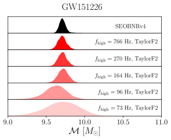
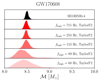
Figure 2: Comparison between the posterior density distributions of the detector’s frame chirp mass when using an IMR approximant (SEOBNRv4) and a inspiral-only PN approximant (TaylorF2) with different values of $f_{\rm high}$. For both GW151226 (left panel) and GW170608 (right panel) the results when using the PN approximant are in good agreement with the IMR result.

Finally, to make inferences on the unknown parameters $\bm{\theta}$ for a given event, we use again Bayes’ theorem to compute the posterior probability

$$P(\bm{\theta}|d,\mathcal{H},I)=\frac{P(\bm{\theta}|\mathcal{H},I)P(d|\bm{\theta},\mathcal{H},I)}{P(d|\mathcal{H},I)}\,.$$ (24)

For the prior probability density $P(\bm{\theta}|\mathcal{H},I)$ we follow the choices in Ref. Veitch et al. (2015). The likelihood function $P(d|\bm{\theta},\mathcal{H},I)$ is defined as the distribution of the residuals, assuming they are distributed as Gaussian noise colored by the noise-power spectral-density $S_{n}(f)$ for each detector Veitch et al. (2015):

$$P(d|\bm{\theta},\mathcal{H},I)\propto\exp\left[-\frac{1}{2}\sum_{k}\left\langle h_{k}(\bm{\theta})-d_{k}\middle|h_{k}(\bm{\theta})-d_{k}\right\rangle\right],$$ (25)

where the sum in the above expression is over all the detectors and we define the noise-weighted inner product as  Finn (1992):

$$\left\langle g|h\right\rangle=2\int_{f_{\rm low}}^{f_{{\rm cutoff}}}\frac{\tilde{g}(f)\tilde{h}^{*}(f)+\tilde{g^{*}}(f)\tilde{h}(f)}{S_{n}(f)}\,,$$ (26)

where $\tilde{g}$ and $\tilde{h}$ denote the Fourier transform of $g$ and $h$, respectively. To sample the posterior density functions and compute the evidences we use a nested sampling algorithm as implemented in the LALInference code Veitch et al. (2015) of the LIGO Algorithm Library Suite (LALSuite) LIGO Scientific Collaboration and Virgo Collaboration (2018).

For the minimum frequency in the analysis we use $f_{\rm low}=20$ Hz. On the other hand, as we already discussed, when setting $f_{\rm high}$ we must take into account the fact that EFTGR is expected to break down when $f>f_{\Lambda}$, where we remind that $f_{\Lambda}$ is defined through Eq. (17). Therefore when computing the likelihood function we set $f_{\rm high}<f_{\Lambda}$. When choosing the value of $f_{\rm high}$, one must also take into account the fact that the precise value of the GW frequency $f$ at which the model breaks down is unknown. The choice of $f_{\rm high}$ therefore adds a systematic error in the constraints on $d_{\Lambda}$. To study the impact of this choice we work with several values of $f_{\rm high}$. It is clear that the smaller the ratio $f_{\rm high}/f_{\Lambda}$ is, the more conservative is the bound we place on the EFTGR parameter $\Lambda$.

Assuming that one has a precise measurement of the total mass, for our lowest choice, $f_{\rm high}\approx 0.2f_{\Lambda}$, the effects on the physical observables from the EFTGR corrections are smaller than the GR values for all the data points we use. Moreover, $f_{\rm high}\approx 0.35f_{\Lambda}$ allows the EFTGR effects to be comparable to the GR effect for the highest frequencies included in the analysis, consequently, one may expect significant corrections from the subleading EFTGR terms in this case.

To constrain $d_{\Lambda}$ we perform a Bayesian model selection where we compare, on a given data subset where the EFT analysis can be reliably performed, the hypothesis that the data contains a signal described by the EFTGR model (16) with a given value of $d_{\Lambda}$ against the hypothesis that the signal is described by GR, which corresponds to $d_{\Lambda}=0$. To fix $f_{\rm high}$ we also need to define the mass scale appearing in Eq. (17). Here we choose this mass scale to be given by the median source’s frame mass obtained when using a full inspiral-merger-ringdown (IMR) template in GR. This choice is not unique, however we note that any other choice for this mass scale can be absorbed into a rescaling of $f_{\rm high}$. By considering a range of values for $f_{\rm high}$ we can therefore also incorporate this uncertainty in our results, as we discuss in more detail below.

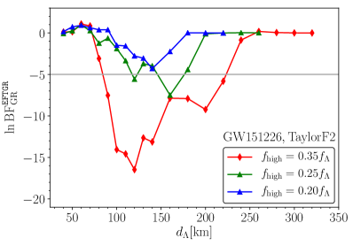
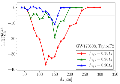
Figure 3: The natural logarithm of the Bayes factor of the EFTGR versus GR waveform model for different choices of $d_{\Lambda}$ (in km) when using the inspiral-only PN waveform model. We use different values for $f_{\rm high}$ when computing the likelihood function (25) to account for the different systematic uncertainties mentioned in the text. To compute $f_{\Lambda}$ we use the median source’s frame total masses obtained with IMR templates as reported in Refs. Abbott et al. (2016b, 2017). We show the results for the two lowest-mass GW events detected so far: GW151226 with total mass $M_{\rm tot}\simeq 22M_{\odot}$ (left panel) and GW170608 with total mass $M_{\rm tot}\simeq 19M_{\odot}$ (right panel). For reference we mark the threshold $\ln B_{\rm GR}^{\rm{\tt EFTGR}}=-5$ with a grey solid curve.

In addition to these difficulties, the EFTGR corrections to the GW phase given by Eq. (16) are only valid in the PN-expanded approximation of the inspiral phase, and do not provide any information about the expected non-GR corrections in the merger-ringdown phase of the signal. Therefore to constrain $d_{\Lambda}$ we employ the Flexible Theory Agnostic (FTA) code developed for LIGO and Virgo analyses Abbott et al. (2018, 2019b), and add the non-GR correction in Eq. (16) to an aligned-spin GR inspiral-only PN waveform model valid up to 3.5PN order. This waveform is artificially set to zero for frequencies $f>f_{\rm ISCO}$, the regime at which the PN expansion is expected to loose significant accuracy. We should emphasize that choosing $f_{\rm ISCO}$ as the frequency cutoff of our waveform model is largely arbitrary, and therefore this specific choice adds another systematic effect in the constraints that we can place on $d_{\Lambda}$. To quantify this uncertainty in Appendix B we also show our results when using an IMR waveform, finding negligible differences.

One might worry that the use of an inspiral-only PN approximant containing an abrupt cutoff at $f_{\rm ISCO}$ might lead to a bias in the measured parameters if part of the post-inspiral signal is loud enough, even when assuming GR Mandel et al. (2014). We have indeed checked that for GW150914 Abbott et al. (2016c), a GW event with a significant signal-to-noise ratio (SNR) in the merger-rigdown part of the signal, using a GR inspiral-only PN template leads to biases in the measured BH masses when compared to the measurement done with an IMR model. However, for low-mass GW events that, in the frequency band of the detectors, are mostly dominated by the inspiral part of the signal, we do not expect this to be a problem. To justify this statement we have checked that for the two lowest-mass binary BH (BBH) events reported thus far by the LIGO and Virgo collaborations, GW151226 Abbott et al. (2016b) and GW170608 Abbott et al. (2017), we indeed find no biases in the measurement of the waveform parameters when using a GR inspiral-only PN waveform model . This can be seen in Fig. 2 where we show the marginalized posterior density distributions for the chirp mass that we obtain when using the inspiral-only PN-approximant TaylorF2 (with $d_{\Lambda}=0$) for different values of $f_{\rm high}$, and compare these results with the posterior obtained when using an IMR template (SEOBNRv4) with $f_{\rm high}=1\,024$ Hz. As expected, the statistical error increases with decreasing $f_{\rm high}$, due to the decreasing SNR, but the measurements when using the IMR template and the inspiral-only PN template are in good agreement. The same conclusion holds for the other parameters of the model. The loss of SNR when $f_{\rm high}\lesssim 200$ Hz is consistent with the fact that for both events $f_{\rm ISCO}\sim 200$ Hz, and therefore, part of the signal is cut whenever $f_{\rm high}\lesssim 200$ Hz. This feature will be important to understand the qualitative behaviour of our results in the next Section. Given these conclusions in what follows we focus our tests on the two longest signals detected so far by LIGO and Virgo, notably GW151226 and GW170608.

IV.2 Bounds on the effective–field-theory extension of General Relativity using GW151226 and GW170608

Using the Bayesian framework presented above we now show that GW151226 and GW170608 can already be used to set meaningful constraints on the parameter $d_{\Lambda}$.

Our main results are summarized in Fig. 3 where we show the natural logarithm of the Bayes factor of the EFTGR hypothesis against GR, $\ln B_{\rm GR}^{\rm{\tt EFTGR}}$. We remind that the EFTGR hypothesis corresponds to the hypothesis that the data are well described by the EFTGR waveform model (16) with a given value of $d_{\Lambda}$ against the hypothesis that the signal is described by GR, i.e., $d_{\Lambda}=0$. We show our results when using an inspiral-only PN approximant in Fig. 3, but similar results hold when using an IMR waveform (see Appendix B for more details). To quantify the systematic error in the uncertainty of the frequency at which the EFTGR model cannot be trusted, we consider different choices of $f_{\rm high}=[0.2,0.25,0.35]f_{\Lambda}$. As mentioned above, to compute $f_{\Lambda}$ we fix the mass scale in Eq. (17) to be the median value for the total BH mass obtained when estimating the parameters with an IMR waveform model in GR as given in Refs. Abbott et al. (2016b, 2017). We could have made other choices for this mass scale, however the uncertainty in the total mass of the system can be absorbed inside the definition of $f_{\rm high}$. For example, using the 90% credible intervals reported in Refs. Abbott et al. (2016b, 2017) we have verified that this would be equivalent to rescaling $f_{\rm high}$ by a factor $\sim 0.96$ and $\sim 1.12$ for the lower and upper limits of the 90% credible intervals, respectively. Taking $f_{\rm high}=0.25f_{\Lambda}$ as our fiducial choice, this variation is smaller than the difference between the three different values of $f_{\rm high}$ that we consider. Therefore by using several values for $f_{\rm high}$ when showing our results we are also taking into account this uncertainty.

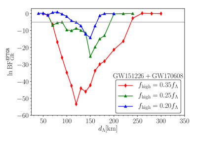
Figure 4: The log Bayes factors of the EFTGR versus GR waveform when combining the results shown in Fig. 3.

Our results show that $\ln B_{\rm GR}^{\rm{\tt EFTGR}}<0$ for a wide range of values for $d_{\rm\Lambda}$, implying that the EFTGR hypothesis is disfavored for some values of $d_{\rm\Lambda}$. The constraints we obtain are similar between the two events, due to their similar total mass. However, for GW170608 one obtains slightly stronger evidence against the EFTGR hypothesis due to the larger SNR of this event when compared with GW151226. Setting a threshold $\ln B_{\rm GR}^{\rm{\tt EFTGR}}\lesssim-5$  to constrain $d_{\Lambda}$, we can draw the strong conclusion that values of $d_{\Lambda}$ between roughly $70$ and $200$ km are strongly disfavored by the data, independently on our choice of $f_{\rm high}$. The evidence against the EFTGR hypothesis is, however, highly dependent on $f_{\rm high}$. This should be expected given that the effect of $d_{\Lambda}$ only appears in the waveform phase (16) at high PN order and therefore, for a given $d_{\Lambda}$, the larger $f_{\rm high}$ the larger the contribution from the non-GR term and the stronger the constraints that we can place.

The qualitative features of our results can be largely understood in terms of two competing effects: (1) for small $d_{\Lambda}$ the Bayes factor asymptotically goes to $B_{\rm GR}^{\rm{\tt EFTGR}}\sim 1$, since the non-GR contribution decreases as $d_{\Lambda}$ becomes smaller, and (2) in the opposite direction, for increasing values of $d_{\Lambda}$, one must also decrease $f_{\rm high}$ and therefore for some large value of $d_{\Lambda}$ the amount of data that we use are no longer sufficient to dig out the signal from the noise, no matter which model we use. Therefore, for some large value of $d_{\Lambda}$ the Bayes factor should also approach $B_{\rm GR}^{\rm{\tt EFTGR}}\sim 1$, as we indeed see in Fig. 3. Due to these two competing effects, we are only able to constrain an interval of values $d^{\rm low}_{\Lambda}<d_{\Lambda}<d^{\rm high}_{\Lambda}$. The lower-limit $d^{\rm low}_{\Lambda}$ in this constraint is more robust against different choices of $f_{\rm high}$, since for large enough $f_{\rm high}$ one is effectively analysing the full signal up to the PN-aproximant frequency cutoff, $f_{\rm ISCO}$. On the other hand, the upper-limit $d^{\rm high}_{\Lambda}$ is obviously quite dependent on the choice that we make for $f_{\rm high}$, since $d^{\rm high}_{\Lambda}$ mostly depends on the maximum value of $f_{\rm high}$ below which the matched-filtered SNR is too small to separate the signal from the noise.

Using Eq. (23), the results presented in Fig. 3 can be combined to improve the constraints on $d_{\Lambda}$. The resulting combined Bayes factors are shown in Fig. 4. One can see that by combining both events the evidence against the EFTGR hypothesis around $d_{\Lambda}\sim 150$ km increases significantly when compared to the constraints obtained with a single event. The importance of combining the information from different GW events is even more striking for the case $f_{\rm high}=0.2f_{\Lambda}$. For that choice of $f_{\rm high}$, GW151226 alone does not give any meaningful constraints, however when combining it with GW170608, one gets strong constraints for values of $d_{\Lambda}$ around $d_{\Lambda}\sim 150$ km. We expect these constraints to further improve as more GW events are observed in the future.

Table 1: Range of values of $d_{\Lambda}$ that are strongly disfavored by GW151226 and GW170608, and when combining both events. To determine these constraints we set the threshold at $\log B_{\rm GR}^{\rm{\tt EFTGR}}\lesssim-5$. We show the constraints for the different choices of $f_{\rm high}$.

Event	$d_{\Lambda}$ [km]
	$f_{\rm high}=0.2f_{\Lambda}$	$f_{\rm high}=0.25f_{\Lambda}$	$f_{\rm high}=0.35f_{\Lambda}$
GW151226	–	$\sim[125,175]$	$\sim[85,225]$
GW170608	$\sim[135,160]$	$\sim[65,190]$	$\sim[65,230]$
Combined	$\sim[120,165]$	$\sim[65,190]$	$\sim[65,235]$

The constraints of the individual and the combined results are summarized in Table 1. Taking into account the systematics entering the choice of $f_{\rm high}$, we conclude that coupling constants around $d_{\Lambda}\sim 150$ km are strongly disfavored. This is in agreement with the prediction made in Ref. Endlich et al. (2017), and can be easily understood from the fact that in this range $d_{\Lambda}/r_{\rm ISCO}\sim\mathcal{O}(1)$ for the BBHs we considered. This regime is the region where the deviations from GR are maximized while still keeping the perturbative control of the EFT. Interestingly, this sets a typical scale that a given event can constrain. Combining the information from more events will therefore not only be important to increase the confidence for or against a given value of $d_{\Lambda}$, but also to increase the range of values of $d_{\Lambda}$ that one can probe and possibly constrain.

Finally, so far we have assumed that $\Lambda^{6}>0$, but as mentioned in Sec. II, there is no strong reason to dismiss the case $\Lambda^{6}<0$. Thus, we have also extended the analysis discussed in this section to the case $\Lambda^{6}<0$ , and have found that when combining the results from both events, the constraints become $1/|\Lambda|\sim[140,160]$ km, $1/|\Lambda|\sim[65,190]$ km and $1/|\Lambda|\sim[65,235]$ km for $f_{\rm high}=[0.2,0.25,0.35]f_{\Lambda}$, respectively.

V Conclusions

We presented the first constraints on the EFTGR proposed in Ref. Endlich et al. (2017), which is described by the action (1), using the two lowest-mass GW events so far detected by LIGO and Virgo. Taking into account the different uncertainties in our analysis, our results show that current observations disfavour coupling constants of the order $d_{\Lambda}\equiv 1/\Lambda\sim 150$ km. The Bayesian method we employed can be easily used to combine information from several observations, and therefore we expect that future GW detections will allow us to further constrain this theory.

Our constraints assumed that, in the regime where $\Lambda\lesssim 1/r_{s}$, the leading order non-GR effect come from the properties of the binary and not modifications from the BH geometry. As argued in Sec. II, the situation may be different for highly spinning BHs in which case, within the soft-UV completion assumption, modifications to the spin-induced BH quadrupole moment may dominate. By adding order one corrections to the GR spin-induced BH quadrupole moment, we have checked that for the events we considered the modifications to the binary dynamics always dominates. This is in agreement with recent work, where it was shown that the spin-induced BH quadrupole moments cannot be well constrained for GW151226 and GW170608 Krishnendu et al. (2019). Constraining the spin-induced BH quadrupole moment with future GW events is an interesting direction that may further improve our constraints.

We focused our analysis to the regime $\Lambda\lesssim 1/r_{s}$. Complementary constraints in the regime $\Lambda\gtrsim 1/r_{s}$, can in principle be obtained from, e.g., measurements of the spin-induced BH quadrupole moment, the tidal Love numbers or measurements of the BH-remnant’s QNMs Cardoso et al. (2018). The events observed by LIGO and Virgo so far have too low SNR to put any constraints in this regime (see Appendix A). In fact, it would be interesting to study how well future detectors on the ground and in space, such as Cosmic Explorer, Einstein Telescope and LISA, can constrain $\Lambda$, not only because BBHs will have much higher SNR, but also much longer inspiral phase, thus making our constraints more robust by choosing a lower value of $f_{\rm high}$.

Although we only showed constraints for $\Lambda$, the same method can be applied to constrain $\tilde{\Lambda}$ and $\Lambda_{-}$, but constraints on the latter will likely require events with a larger SNR and binaries with spinning components for which the effect of the terms $\tilde{\mathcal{C}}^{2}$ and $\tilde{\mathcal{C}}\mathcal{C}$ is expected to be non-negligible Endlich et al. (2017). It would also be interesting to analyse EFTGR with cubic terms in the Riemann tensor, though they are theoretically disfavored.

Finally, our results relied on computing the leading-order non-GR PN correction, but stronger constraints could in principle be obtained by building IMR waveforms for these EFTs. This will require numerical simulations of BBHs in the EFTGR. Numerical simulations could be done along the lines of the proposals in Refs. Okounkova et al. (2017); Witek et al. (2019); Okounkova et al. (2019b, a) where significant progress has been made to perform numerical simulations of BH mergers in an EFT extension of gravity with higher-derivative operators and an additional light degree of freedom.

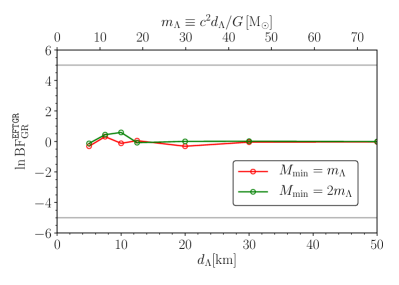
Figure 5: The natural logarithm of the Bayes factors of the EFTGR versus GR waveform for GW170608 in the regime where $d_{\Lambda}\lesssim M$, with $M$ the mass of either BH in the binary, with corresponding $m_{\Lambda}$ shown in the top $x$-axis, when using the PN waveform model. We fix the minimum mass $M_{\rm min}$ in the priors for the BH masses such that $d_{\Lambda}<M$ is always satisfied in the GW template. To account for the systematic uncertainty in the validity of the waveform model, we use different values for the minimum mass in the prior $M_{\rm min}$ as shown by the different curves.

Appendix A Finite-size effects for $\Lambda\gtrsim 1/r_{s}$

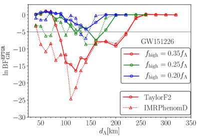
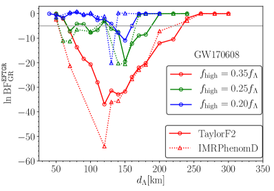
Figure 6: Same as Fig. 3, but also showing the case where we use an IMR waveform model (IMRPhenomD). For the IMR model the EFTGR correction is taped at the merger frequency that we take to be the peak of the waveform’s amplitude

.

As explained in Sec. II, in the regime where $\Lambda\gtrsim 1/r_{s}$, or equivalently $d_{\Lambda}\lesssim M$, with $M$ the mass of either BH in the binary, the modifications to the GW template are mainly associated to modifications of the BH geometry. For this case, the leading-order modifications in the inspiral phase come from a modified BH spin-induced quadrupole moment and non-vanishing tidal Love number Endlich et al. (2017); Cardoso et al. (2018).

Within the PN expansion, the influence of the spin-induced quadrupole moment enters the GW phase at 2PN order whereas the leading-order tidal Love number enters at 5PN order (see, e.g., Ref. Blanchet (2014)). By inserting the explicit expressions for the BH spin-induced quadrupole moment and tidal Love number found in Ref. Cardoso et al. (2018) in a PN template, we can therefore check whether we can impose any constraints in this regime. For simplicity we only consider the $\Lambda$ term in the action (1), but results would be similar for the other terms. We also only consider GW170608 since this event has a larger SNR than GW151226.

We used the same Bayesian model selection procedure presented in Sec. IV, except that now no constraints need to be imposed on the highest frequency in the data. Instead, since we are considering the regime $d_{\Lambda}\lesssim M$, we define a mass associated with $\Lambda$ given by $m_{\Lambda}\equiv\Lambda^{-1}$ and impose a minimum mass $M_{\rm min}$ in the prior probabilities of the BH masses such that only masses satisfying $M_{\rm min}\geq m_{\Lambda}$ are considered in the analysis. This ensures that $d_{\Lambda}<M$ is always satisfied. Our results are shown in Fig. 5. They confirm that, independently on $M_{\rm min}$, there is no preference for either GR or the EFTGR model. Therefore no constraints can be imposed in this regime.

Appendix B Constraints when using an inspiral-meger-ringdown waveform

In this appendix we show that similar constraints to the ones shown in the main text can also be obtained with an IMR model. For the EFTGR waveform IMR model we include the non-GR correction in Eq. (16) in the inspiral phase of the waveform and, since the corrections in the merger-ringdown are unknown, we taper the correction to zero at the merger frequency, taken to be the peak of the waveform’s amplitude. We perform the test using the FTA code developed and employed in the analyses of Refs. Abbott et al. (2018, 2019b).

The results obtained when using an IMR model (IMRPhenomD) are shown in Fig. 6. For comparison we also show the results obtained with an inpiral-only PN waveform (TaylorF2), already shown in Fig. 3. We find that the range of values of $d_{\Lambda}$ for which the GR waveform is preferred over the EFTGR one when using the IMR waveform is similar to the one obtained when using an inspiral-only PN waveform (TaylorF2), the main difference being that for $d_{\Lambda}\lesssim 150$ km the constraints obtained with the IMR model are slightly stronger. This is no surprise given that this value of $d_{\Lambda}$ is close to the approximate location of the final BH ISCO for the BBH systems we consider. For $d_{\Lambda}\gtrsim 150$ km both the IMR and inspiral-only PN results should agree given that our choice for $f_{\rm high}$ satisfies $f_{\rm high}\lesssim f_{\rm ISCO}$. On the other hand, for $d_{\Lambda}\lesssim 150$ km the IMR waveform model gives slightly stronger constraints due to the inclusion of non-GR corrections at frequencies above $f_{\rm ISCO}$ in the waveform. However, independently of whether we use the IMR or the inspiral-only PN approximant the range of values $d_{\Lambda}$ that we constrain does not change significantly.

References

- Abbott et al. (2019a) B. P. Abbott et al. (LIGO Scientific, Virgo), Phys. Rev. X9, 031040 (2019a), arXiv:1811.12907 [astro-ph.HE] .
- Abbott et al. (2016a) B. P. Abbott et al. (Virgo, LIGO Scientific), Phys. Rev. Lett. 116, 221101 (2016a), arXiv:1602.03841 [gr-qc] .
- Yunes et al. (2016) N. Yunes, K. Yagi, and F. Pretorius, Phys. Rev. D94, 084002 (2016), arXiv:1603.08955 [gr-qc] .
- Abbott et al. (2018) B. P. Abbott et al. (LIGO Scientific, Virgo), (2018), arXiv:1811.00364 [gr-qc] .
- Abbott et al. (2019b) B. P. Abbott et al. (LIGO Scientific, Virgo), (2019b), arXiv:1903.04467 [gr-qc] .
- Will (2014) C. M. Will, Living Rev. Rel. 17, 4 (2014), arXiv:1403.7377 [gr-qc] .
- Baker et al. (2015) T. Baker, D. Psaltis, and C. Skordis, Astrophys. J. 802, 63 (2015), arXiv:1412.3455 [astro-ph.CO] .
- Baker et al. (2019) T. Baker et al., (2019), arXiv:1908.03430 [astro-ph.CO] .
- Berti et al. (2015) E. Berti et al., Class. Quant. Grav. 32, 243001 (2015), arXiv:1501.07274 [gr-qc] .
- Arun et al. (2006) K. G. Arun, B. R. Iyer, M. S. S. Qusailah, and B. S. Sathyaprakash, Phys. Rev. D74, 024006 (2006), arXiv:gr-qc/0604067 [gr-qc] .
- Yunes and Pretorius (2009) N. Yunes and F. Pretorius, Phys. Rev. D80, 122003 (2009), arXiv:0909.3328 [gr-qc] .
- Mishra et al. (2010) C. K. Mishra, K. G. Arun, B. R. Iyer, and B. S. Sathyaprakash, Phys. Rev. D82, 064010 (2010), arXiv:1005.0304 [gr-qc] .
- Li et al. (2012) T. G. F. Li, W. Del Pozzo, S. Vitale, C. Van Den Broeck, M. Agathos, J. Veitch, K. Grover, T. Sidery, R. Sturani, and A. Vecchio, Phys. Rev. D85, 082003 (2012), arXiv:1110.0530 [gr-qc] .
- Agathos et al. (2014) M. Agathos, W. Del Pozzo, T. G. F. Li, C. Van Den Broeck, J. Veitch, and S. Vitale, Phys. Rev. D89, 082001 (2014), arXiv:1311.0420 [gr-qc] .
- Nair et al. (2019) R. Nair, S. Perkins, H. O. Silva, and N. Yunes, (2019), arXiv:1905.00870 [gr-qc] .
- Endlich et al. (2017) S. Endlich, V. Gorbenko, J. Huang, and L. Senatore, JHEP 09, 122 (2017), arXiv:1704.01590 [gr-qc] .
- Gruzinov and Kleban (2007) A. Gruzinov and M. Kleban, Class. Quant. Grav. 24, 3521 (2007), arXiv:hep-th/0612015 [hep-th] .
- Bellazzini et al. (2016) B. Bellazzini, C. Cheung, and G. N. Remmen, Phys. Rev. D93, 064076 (2016), arXiv:1509.00851 [hep-th] .
- Goroff and Sagnotti (1986) M. H. Goroff and A. Sagnotti, Nucl. Phys. B266, 709 (1986).
- Camanho et al. (2016) X. O. Camanho, J. D. Edelstein, J. Maldacena, and A. Zhiboedov, JHEP 02, 020 (2016), arXiv:1407.5597 [hep-th] .
- Reall and Santos (2019) H. S. Reall and J. E. Santos, JHEP 04, 021 (2019), arXiv:1901.11535 [hep-th] .
- Bambi (2014) C. Bambi, Phys. Lett. B730, 59 (2014), arXiv:1401.4640 [gr-qc] .
- Reynolds (2014) C. S. Reynolds, Space Sci. Rev. 183, 277 (2014), arXiv:1302.3260 [astro-ph.HE] .
- Okounkova et al. (2017) M. Okounkova, L. C. Stein, M. A. Scheel, and D. A. Hemberger, Phys. Rev. D96, 044020 (2017), arXiv:1705.07924 [gr-qc] .
- Witek et al. (2019) H. Witek, L. Gualtieri, P. Pani, and T. P. Sotiriou, Phys. Rev. D99, 064035 (2019), arXiv:1810.05177 [gr-qc] .
- Okounkova et al. (2019a) M. Okounkova, L. C. Stein, M. A. Scheel, and S. A. Teukolsky, (2019a), arXiv:1906.08789 [gr-qc] .
- Vainshtein (1972) A. I. Vainshtein, Phys. Lett. 39B, 393 (1972).
- Cardoso et al. (2018) V. Cardoso, M. Kimura, A. Maselli, and L. Senatore, Phys. Rev. Lett. 121, 251105 (2018), arXiv:1808.08962 [gr-qc] .
- Goldberger and Rothstein (2006) W. D. Goldberger and I. Z. Rothstein, Phys. Rev. D73, 104029 (2006), arXiv:hep-th/0409156 [hep-th] .
- Damour et al. (1998) T. Damour, B. R. Iyer, and B. S. Sathyaprakash, Phys. Rev. D57, 885 (1998), arXiv:gr-qc/9708034 [gr-qc] .
- Buonanno et al. (2009) A. Buonanno, B. Iyer, E. Ochsner, Y. Pan, and B. S. Sathyaprakash, Phys. Rev. D80, 084043 (2009), arXiv:0907.0700 [gr-qc] .
- Zimmerman et al. (2019) A. Zimmerman, C.-J. Haster, and K. Chatziioannou, (2019), arXiv:1903.11008 [astro-ph.IM] .
- Veitch et al. (2015) J. Veitch et al., Phys. Rev. D91, 042003 (2015), arXiv:1409.7215 [gr-qc] .
- Finn (1992) L. S. Finn, Phys. Rev. D46, 5236 (1992), arXiv:gr-qc/9209010 [gr-qc] .
- LIGO Scientific Collaboration and Virgo Collaboration (2018) LIGO Scientific Collaboration and Virgo Collaboration, “LALSuite software,” (2018).
- Abbott et al. (2016b) B. P. Abbott et al. (Virgo, LIGO Scientific), Phys. Rev. Lett. 116, 241103 (2016b), arXiv:1606.04855 [gr-qc] .
- Abbott et al. (2017) B. P. Abbott et al. (Virgo, LIGO Scientific), Astrophys. J. 851, L35 (2017), arXiv:1711.05578 [astro-ph.HE] .
- Khan et al. (2016) S. Khan, S. Husa, M. Hannam, F. Ohme, M. Pürrer, X. Jiménez Forteza, and A. Bohé, Phys. Rev. D93, 044007 (2016), arXiv:1508.07253 [gr-qc] .
- Bohé et al. (2017) A. Bohé et al., Phys. Rev. D95, 044028 (2017), arXiv:1611.03703 [gr-qc] .
- Mandel et al. (2014) I. Mandel, C. P. L. Berry, F. Ohme, S. Fairhurst, and W. M. Farr, Class. Quant. Grav. 31, 155005 (2014), arXiv:1404.2382 [gr-qc] .
- Abbott et al. (2016c) B. P. Abbott et al. (Virgo, LIGO Scientific), Phys. Rev. Lett. 116, 061102 (2016c), arXiv:1602.03837 [gr-qc] .
- Jeffreys (1939) H. Jeffreys, The Theory of Probability (Oxford University press, Oxford, 1939).
- Krishnendu et al. (2019) N. V. Krishnendu, M. Saleem, A. Samajdar, K. G. Arun, W. Del Pozzo, and C. K. Mishra, (2019), arXiv:1908.02247 [gr-qc] .
- Okounkova et al. (2019b) M. Okounkova, M. A. Scheel, and S. A. Teukolsky, Phys. Rev. D99, 044019 (2019b), arXiv:1811.10713 [gr-qc] .
- Blanchet (2014) L. Blanchet, Living Rev. Rel. 17, 2 (2014), arXiv:1310.1528 [gr-qc] .