String scale interacting dark matter from $\pi_{1}$

Abstract

We show that in a wide class of string derived models of particle physics, heavy string modes with masses around the GUT scale can serve as a viable dark matter candidate. These heavy string modes wind around specific cycles in the extra-dimensional space, closely related to the fundamental group $\pi_{1}$. As a consequence of a non-trivial $\pi_{1}$, there is an exact discrete symmetry that stabilizes such winding strings. The dark matter candidate couples to the Standard Model via gravity and via the exchange of heavy string states. We find that, for reasonable values of the string coupling, our dark matter candidate can be produced in sizable amounts via freeze-in. Our scheme applies to many string constructions, including Calabi–Yau compactifications, and can be tested against constraints from the CMB.

1 Introduction

Successful models for particle dark matter consist of two main ingredients: the dark matter candidate that interacts with the Standard Model (SM) only very weakly, and a mechanism that ensures its relative longevity. In most instances, a $\mathbbm{Z}_{2}$ symmetry is invoked to keep the dark matter particle from decaying. Moreover, if the model is supposed to explain the presently observed dark matter relic density, one needs to make sure that it is produced in sufficient quantities in the early universe. The prime example for a dark matter candidate is the weakly interacting massive particle (WIMP), which is in thermal equilibrium with the thermal plasma and “freezes out” after dropping out of equilibrium Kolb:1990vq ; Jungman:1995df . However, it has been demonstrated that a dark matter species may also be produced thermally in sizable quantities even if it never attains thermal equilibrium (“freeze-in”) Hall:2009bx . More specifically, it has become clear that freeze-in production can work with extremely heavy dark matter candidates (with masses above the GUT scale) and couplings that are suppressed by $1/m_{\mathrm{Pl}}^{2}$, a framework that is known as Planckian interacting dark matter (PIDM) Garny:2015sjg ; Garny:2017kha . This observation is intriguing from the viewpoint of string model building, for a number of reasons. On the one hand, it is expected that the lightest massive string states have masses around the string scale, and that there are, apart from gravity, stringy interactions between these states and the massless states of the Standard Model that are suppressed by $1/m_{\mathrm{s}}^{2}$. Furthermore, there is a wide class of string models that have a stabilizing symmetry built in Kogan:1986fx , e.g. an abelian $\mathbbm{Z}_{2}$ symmetry Ramos-Sanchez:2018edc . The goal of this paper is to show that this class of string models can yield viable models of dark matter. As an explicit example, we consider the framework of heterotic string theory with six extra dimensions compactified on a special class of orbifolds but our scheme is valid more generally. In particular, our dark matter candidate is given by a closed string state that winds around a certain cycle in the extra-dimensional compact space. Then, its stability can be ensured via an exact discrete symmetry that originates from the topological property of certain compactification spaces to be non-simply connected. Consequently, the discrete symmetry is classically exact and can potentially be broken only non-perturbatively due to a discrete anomaly Banks:1991xj ; Lee:2011dya . This stable string state is generically very heavy (with a mass at the compactification or GUT scale) and interacts with the massless states in the plasma not only via gravity, but also via the exchange of other heavy winding modes.

Figure 1: Dominant dark matter production by the exchange of a mediator field $M$. Note that the dark matter particle is stabilized by an odd $\mathbbm{Z}_{4}$ charge, while Standard Model fields carry even $\mathbbm{Z}_{4}$ charges and the mediator is uncharged. Importantly, the existence of such a stabilizing discrete symmetry is a direct consequence from the extra dimensions of string theory.

2 Interactions between dark matter and the Standard Model

In this section, we will examine which couplings between the dark matter candidate and the particles of the Standard Model can arise at the renormalizable level. To be specific, we consider a string model compactified on the so-called $\mathbbm{Z}_{2}\times\mathbbm{Z}_{2}$-5-1 orbifold in the classification of ref. Fischer:2012qj . However, our findings easily carry over to other orbifold geometries and also to other string compactifications, cf. appendix A for further details. In this model, the dark matter candidate is stabilized by an exact $\mathbbm{Z}_{4}$ symmetry that originates from string selection rules Ramos-Sanchez:2018edc , which in turn are related to topological properties of the compact orbifold space. It should be noted that all massless strings, especially those for the Standard Model particles, have even $\mathbbm{Z}_{4}$ charges, while the DM particles carry odd charges. Hence, the $\mathbbm{Z}_{4}$ has a $\mathbbm{Z}_{2}$ subgroup with precisely the charge assignment needed for dark matter parity and the lightest string with odd $\mathbbm{Z}_{2}$ charge is stable. Now, one has to examine the model further, in order to identify all allowed stringy couplings of the DM particle to the Standard Model. Since we are dealing with a supersymmetric setup, one needs to distinguish between couplings from the Kähler potential and those from the superpotential.

In most instances, the coupling of dark matter to the SM is dominated by $2\rightarrow 2$ scattering. Hence, due to the constraining $\mathbbm{Z}_{4}$ symmetry, the most general coupling looks like the left diagram in figure 1. At tree level, one can boil that down to the exchange of mediator fields $M$, cf. the right diagram in figure 1. What are possible mediator fields? One example are gravitational interactions, where the exchanged particle is the graviton. This case has been studied extensively in the PIDM program Garny:2015sjg ; Garny:2017kha and, as we will see, will give in our setup a contribution that is in general subdominant. However, it turns out that once interactions from string theory are considered, there are additional stringy mediators that can be exchanged and dominate the coupling between DM and the SM. These mediators are also winding strings but with vanishing $\mathbbm{Z}_{4}$ charges. Hence, at generic points in string moduli space they are very massive. On the other hand, they have the generic feature to couple to the winding dark matter candidate and to Standard Model matter under the assumption that the SM matter is localized appropriately in the extra-dimensional orbifold space, cf. appendix A. The exact realizations of winding dark matter, winding mediators and localized SM matter fields depend on the specific string model. However, instead of discussing a full string realization, we consider a very generic string setting as presented in table 1. Consequently, our findings will be rather generic for a wide class of string constructions.

	superfield	type of closed string	$\mathbbm{Z}_{4}$ charge
SM	$\Phi_{i}=(f_{i},\tilde{f}_{i})$	localized	0 or 2
DM	$\Phi_{\mathrm{DM}}=(\chi,\varphi)$	$\tau$-winding	1
	$\Phi_{\mathrm{DM}}^{\prime}=(\chi^{\prime},\varphi^{\prime})$	$-\tau$-winding	3
mediator	$\Phi_{\mathrm{M}}=(\chi_{\mathrm{M}},M)$	winding	0
	$V^{\mathrm{(M)}}=(V_{\mu},\lambda)$	winding	0

Table 1: Summary of the relevant fields for SM, DM and mediator and their corresponding types of strings (i.e. localized strings, $\tau$-winding strings or general winding strings). $\Phi_{\mathrm{DM}}^{\prime}$ denotes the mass partner of the dark matter multiplet $\Phi_{\mathrm{DM}}$.

2.1 Kähler potential terms

If (at least part of) the massless Standard Model matter is localized in the extra-dimensional compact space, there is a set of mediators that can couple to both, the dark matter candidate and the Standard Model. In our concrete setting, there are three types of mediator strings, where each of them potentially couples to a different subset of SM matter. In what follows, we will make the simplifying assumption that all three have the same mass and couplings, such that one can effectively work with one mediator $V^{\mathrm{(M)}}$. As we show in appendix A.3, the mediator field originates from a massive string state that necessarily carries both Kaluza–Klein momentum and winding. Moreover, we shall see later on that variations of the coupling strengths do not have a large impact on our results. Let us now examine the coupling of dark matter to a localized Standard Model particle $\Phi_{i}$. Then, the most general Kähler potential consistent with gauge invariance and the stringy $\mathbbm{Z}_{4}$ symmetry for the coupling of the Standard Model to the mediator reads

$$K_{\mathrm{SM}}~{}\supset~{}\Phi_{i}^{\dagger}\left[\mathrm{e}^{2g_{1}V^{\mathrm{(M)}}}+\frac{g_{1}^{\prime}}{\Lambda}\left(\Phi_{\mathrm{M}}+\Phi_{\mathrm{M}}^{\dagger}\right)+\frac{\mathrm{i}g_{1}^{\prime\prime}}{\Lambda}\left(\Phi_{\mathrm{M}}-\Phi_{\mathrm{M}}^{\dagger}\right)\right]\Phi_{i}\;.$$ (1)

Here, we observe that only the coupling to the vector field $V^{\mathrm{(M)}}=(V_{\mu},\lambda)$ with coupling $g_{1}$ is renormalizable, hence all other terms will be dropped. Therefore, we consider only the coupling of the mediator vector superfield $V^{(\mathrm{M})}$ to the dark matter candidates $\Phi_{\mathrm{DM}}$ and $\Phi_{\mathrm{DM}}^{\prime}$ in the dark matter Kähler potential

$$K_{\mathrm{DM}}~{}\supset~{}\Phi_{\mathrm{DM}}^{\dagger}\,\mathrm{e}^{2g_{2}V^{\mathrm{(M)}}}\Phi_{\mathrm{DM}}+\Phi_{\mathrm{DM}}^{\prime\dagger}\,\mathrm{e}^{-2g_{2}V^{\mathrm{(M)}}}\Phi_{\mathrm{DM}}^{\prime}\;,$$ (2)

see appendix A.3 for the stringy origin of these couplings. Let us parameterize the SM chiral multiplets as $\Phi_{i}=(f_{i},\tilde{f}_{i})$ and the dark matter multiplets as $\Phi_{\mathrm{DM}}=(\chi,\varphi)$ and $\Phi_{\mathrm{DM}}^{\prime}=(\chi^{\prime},\varphi^{\prime})$. The relevant Lagrangian for the $2\rightarrow 2$ production of dark matter from the $D$-terms of the Kähler potentials reads

$$\mathcal{L}~{}\supset ~{}K_{\mathrm{SM}}\left.\vphantom{\int}\!\right|_{D}+K_{\mathrm{DM}}\left.\vphantom{\int}\!\right|_{D}$$ (3)

$$~{}\supset ~{}g_{1}V^{(\mathrm{M})}_{\mu}\left[\left(\overline{f}_{i}\overline{\sigma}^{\mu}f_{i}+2\mathrm{i}\tilde{f}_{i}^{\dagger}\partial_{\mu}\tilde{f}_{i}\right)+g_{2}\left(\overline{\chi}\,\overline{\sigma}^{\mu}\chi+2\mathrm{i}\varphi^{\dagger}\partial_{\mu}\varphi\right)\right]$$

$$+\sqrt{2}g_{1}\left(\tilde{f}_{i}\overline{\lambda}\,\overline{f}_{i}+\tilde{f}_{i}^{\dagger}\lambda f_{i}\right)+\sqrt{2}g_{2}\left(\varphi\overline{\lambda}\overline{\chi}+\varphi^{\dagger}\lambda\chi\right)+\begin{pmatrix}\chi\leftrightarrow\chi^{\prime}\\ \varphi\leftrightarrow\varphi^{\prime}\\ g_{2}\leftrightarrow-g_{2}\end{pmatrix}\;.$$ (4)

Additionally, there is a four-scalar vertex coming from the kinetic term of the mediator multiplet. The Lagrangian coming from the auxiliary field in $V^{(\mathrm{M})}$ reads

$$\mathcal{L}_{(D_{\mathrm{M}})}~{}=~{}\frac{1}{2}D_{\mathrm{M}}^{2}+g_{1}D_{\text{M}}|\tilde{f}_{i}|^{2}+g_{2}D_{\mathrm{M}}|\varphi|^{2}-g_{2}D_{\mathrm{M}}|\varphi^{\prime}|^{2}+\dots\;,$$ (5)

which, upon setting the auxiliary field $D_{\mathrm{M}}$ on-shell, yields

$$\mathcal{L}_{(D_{\mathrm{M}})}~{}=~{}-\frac{1}{2}\left(g_{1}|\tilde{f}_{i}|^{2}+g_{2}|\varphi|^{2}-g_{2}|\varphi^{\prime}|^{2}\right)^{2}+\dots\;,$$ (6)

and, hence, we obtain a four-scalar vertex with a coupling $g_{1}g_{2}$. Then, we find that at tree level the relevant channels for the non-gravitational interactions of dark matter with the Standard Model are given by the processes shown in figures 2–7. There, we present the production channels for the dark matter multiplet $\Phi_{\mathrm{DM}}$, analogous diagrams exist also for its partner multiplet $\Phi_{\mathrm{DM}}^{\prime}$.

Let us briefly discuss the conceivable range of values for the couplings $g_{1}$ and $g_{2}$. In supersymmetric gauge theories, each gauge coupling is given by a gauge kinetic function $f$. For example, in the case of the $\mathrm{U}(1)$ associated with the mediator field $V_{\mu}^{(\text{M})}$ we have

$$f_{\mathrm{U}(1)}~{}=~{}S+\Delta_{\mathrm{U}(1)}(T_{i},U_{i})\;,$$ (7)

where $S$ is the heterotic axio-dilaton and the threshold correction $\Delta_{\mathrm{U}(1)}$ is a stringy one-loop contribution that is in general a complicated function of the geometric moduli $T_{i}$ and $U_{i}$, see ref. Dixon:1990pc . However, for the non-factorizable orbifold we are considering, the precise form of $\Delta_{\mathrm{U}(1)}$ is unknown. Still, we expect that by varying the geometric moduli, one can generate wide ranges of effective couplings for the mediator $\mathrm{U}(1)$. The couplings of the Standard Model gauge group follow a similar pattern. However, the threshold corrections $\Delta_{\mathrm{SM}}$ for the Standard Model have in general a different dependence on the geometric moduli than $\Delta_{\mathrm{U}(1)}$. Hence, it is conceivable that the mediator couplings can be varied without spoiling the unification of the Standard Model gauge couplings.

Figure 2: $\chi\overline{\chi}\leftrightarrow f_{i}\overline{f}_{i}$

Figure 3: $\chi\overline{\chi}\leftrightarrow\tilde{f}_{i}^{\dagger}\tilde{f}_{i}$

Figure 4: $\varphi^{\dagger}\varphi\leftrightarrow\tilde{f}_{i}^{\dagger}\tilde{f}_{i}$

Figure 5: $\varphi^{\dagger}\varphi\leftrightarrow\tilde{f}_{i}^{\dagger}\tilde{f}_{i}$

Figure 6: $\varphi^{\dagger}\varphi\leftrightarrow f_{i}\overline{f}_{i}$

Figure 7: $\varphi^{\dagger}\chi\leftrightarrow\tilde{f}_{i}^{\dagger}f_{i}$

2.2 Superpotential terms

In addition to the Kähler terms, there can also arise couplings from the superpotential. In particular, it is possible to couple a mediator, residing in a chiral multiplet, to the Standard Model via Higgs portal and neutrino-portal-like terms. If we make the assumption that the mediator $\Phi_{\mathrm{M}}$ couples to all three generations of lepton doublets $L$ with the same coupling constant $\lambda_{N}$, the terms containing the mediator in the corresponding superpotential read

$$\mathcal{W}~{}= ~{}\mathcal{W}_{\mathrm{M}}+\mathcal{W}_{\mathrm{DM}}+\mathcal{W}_{\mathrm{Higgs-portal}}+\mathcal{W}_{\mathrm{neutrino-portal}}$$ (8)

$$~{}= ~{}\frac{m_{\mathrm{M}}}{2}\,\Phi_{\mathrm{M}}^{2}+\frac{\lambda_{\mathrm{M}}}{3}\,\Phi_{\mathrm{M}}^{3}+\frac{m_{\mathrm{DM}}}{2}\,\Phi_{\mathrm{DM}}\,\Phi_{\mathrm{DM}}^{\prime}+\lambda_{\mathrm{DM}}\,\Phi_{\mathrm{M}}\,\Phi_{\mathrm{DM}}\,\Phi_{\mathrm{DM}}^{\prime}$$

$$~{}+\lambda_{\mathrm{H}}\,\Phi_{\mathrm{M}}\,\widehat{H}_{u}\,\widehat{H}_{d}+\lambda_{\mathrm{N}}\,\Phi_{\mathrm{M}}\,\widehat{H}_{u}\,\widehat{L}\;,$$ (9)

where we used the SM superfields $\widehat{H}_{u,d}=(\widetilde{H}_{u,d},H_{u,d})$ for the Higgses and $\widehat{L}=(\ell,\tilde{\ell})$ for the lepton doublet(s). For processes involving the exchange of a mediator, we are interested in the 3-point interactions that arise from this choice for $\mathcal{W}$. Additionally, there is also a four-scalar interaction of two dark matter scalars and two SM scalars. However, in order for the stringy couplings to exist, the Higgs field must be localized. For the neutrino portal, the Higgs field has to live at the same fixed point as the lepton doublet it is supposed to couple to; if these fields live at different fixed points in the same sector the couplings are suppressed, and if they live in another twisted sector the couplings are completely absent. Similar terms then exist for the coupling of the mediator to the dark matter candidate. It turns out that if the couplings $\lambda_{H}$ and $\lambda_{N}$ are chosen to be of the same order as the Kähler couplings $g_{1,2}$, the contribution of the superpotential couplings to the dark matter production rate is not qualitatively different from the contribution of the Kähler potential, but numerically a little bit lower. Moreover, as discussed above, the existence of the neutrino portal couplings requires an specific localization of the lepton and Higgs fields, which is model dependent. For these reasons, and because models with localized Higgs pairs have a less appealing phenomenology, we will not push any further in this direction and consider Kähler terms only by assuming the Higgs field to originate from the bulk.

3 Dark matter production

Although the dark matter candidate is too heavy to be in thermal equilibrium, it can still be produced thermally via freeze-in. The production of dark matter is then governed by the Boltzmann equation

$$\dot{n}+3H(t)\,n~{}=~{}-\left\langle\sigma_{\mathrm{eff}}v\right\rangle\left(n^{2}-n_{\mathrm{eq}}^{2}\right)\;.$$ (10)

Here, $n$ is the number density of all states in the dark matter sector, in other words $n=n_{\chi}+n_{\varphi}+n_{\overline{\chi}}+n_{\varphi^{\dagger}}+n_{\chi^{\prime}}+n_{\varphi^{\prime}}+n_{\overline{\chi}^{\prime}}+n_{\varphi^{{}^{\prime}\dagger}}$. On the right hand side of equation (10), $\left\langle\sigma_{\mathrm{eff}}v\right\rangle$ is the effective thermally averaged cross section for the various $2\rightarrow 2$ dark matter production channels, taking also coannihilations into account Gondolo:1990dk ; Edsjo:1997bg . Using $m_{i}=m_{\chi}$ it reads

$$\left\langle\sigma_{\mathrm{eff}}v\right\rangle~{}=~{}\frac{T}{n_{\mathrm{eq}}^{2}}\frac{1}{8\pi^{4}}\int_{4m_{\chi}^{2}}^{\infty}\mathrm{d}s\sqrt{s}\,p^{2}\,\left(\sum_{i,j}g_{i}g_{j}\sigma_{ij}(s)\right)\,K_{1}\left(\frac{\sqrt{s}}{T}\right)\;.$$ (11)

Here, $g_{i}$ counts the internal degrees of freedom of each species $i$ (where $g_{i}=2$ for a Weyl fermion and $g_{i}=1$ for a real scalar), and the summation indices $i$ and $j$ run over all fields in the dark sector. Furthermore, $p=\sqrt{s/4-m_{\chi}^{2}}$, and $K_{1}$ is the modified Bessel function of the second kind of order 1. The equilibrium density $n_{\mathrm{eq}}$ is given by

$$n_{\mathrm{eq}}~{}=~{}\sum_{i}\frac{T}{2\pi^{2}}g_{i}\,m_{i}^{2}K_{2}\left(\frac{m_{i}}{T}\right)~{}=~{}\frac{4T}{\pi^{2}}\,m_{\chi}^{2}K_{2}\left(\frac{m_{\chi}}{T}\right)\;,$$ (12)

where $K_{2}$ is the modified Bessel function of the second kind of order 2. The cross sections $\sigma_{ij}$ correspond to the various possible scattering processes shown in figures 2–7, and are given by

$$\sigma_{ij}~{}=~{}\frac{1}{16\pi s\left(s-4m_{\chi}^{2}\right)}\int_{t_{-}}^{t_{+}}\mathrm{d}t\left|\mathcal{M}_{ij}(t)\right|^{2}\;.$$ (13)

Here, $t_{\pm}=-\left(\sqrt{s/4}\mp\sqrt{s/4-m_{\chi}^{2}}\right)^{2}$ and $\mathcal{M}_{ij}(t)$ denote the matrix elements for the respective process. In what follows, we focus on the case with bulk Higgs fields and, hence, there are no contributions from the superpotential. Then, the non-vanishing cross sections $\sigma_{ij}$ are given by

$$\sigma_{\chi\overline{\chi}}~{}= ~{}\sigma_{\chi\overline{\chi}\rightarrow f_{i}\overline{f}_{i}}+\sigma_{\chi\overline{\chi}\rightarrow\tilde{f}_{i}\tilde{f}_{i}^{\dagger}}$$ (14)

$$\sigma_{\varphi\varphi^{\dagger}}~{}= ~{}\sigma_{\varphi\varphi^{\dagger}\rightarrow f_{i}\overline{f}_{i}}+\sigma_{\varphi\varphi^{\dagger}\rightarrow\tilde{f}_{i}\tilde{f}_{i}^{\dagger}}$$ (15)

$$\sigma_{\chi\varphi^{\dagger}}~{}= ~{}\sigma_{\chi\varphi^{\dagger}\rightarrow f_{i}\tilde{f}_{i}^{\dagger}}$$ (16)

$$\sigma_{\overline{\chi}\varphi}~{}= ~{}\sigma_{\chi\varphi^{\dagger}}\;,$$ (17)

plus the corresponding terms for $\chi^{\prime},\varphi^{\prime}$. Moreover, it holds that $\sigma_{ij}=\sigma_{ji}$. With these preparations in place, one can perform the thermal averaging eq. (11) numerically (cf. figure 8) and turn one’s attention to the Boltzmann equation.

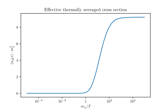
Figure 8: The effective thermally averaged cross section for a mediator mass $m_{\mathrm{M}}=1.8\,m_{\chi}$ and all couplings set to unity. Observe how the cross section approaches a constant value for $T\ll m_{\chi}$.

As the actual density in the freeze-in case is always much smaller than the equilibrium one, the full Boltzmann equation (10) can be approximated to sufficient accuracy by neglecting $n^{2}$ compared to $n_{\mathrm{eq}}^{2}$ on the right hand side of equation (10) and hence using

$$\dot{n}+3H(t)\,n~{}=~{}\left\langle\sigma_{\mathrm{eff}}v\right\rangle\,n_{\mathrm{eq}}^{2}\;.$$ (18)

Proceeding like in ref. Garny:2015sjg , one can now simplify the discussion by introducing the dimensionless abundance $X=na^{3}/T_{\mathrm{rh}}^{3}$ in terms of the scale factor $a$ and the reheating temperature $T_{\mathrm{rh}}$, such that equation (18) can be integrated to yield

$$X_{\mathrm{f}}~{}=~{}\frac{1}{T_{\mathrm{rh}}^{3}}\int_{1}^{\infty}\mathrm{d}a\frac{a^{2}}{H(a)}\left\langle\sigma_{\mathrm{eff}}v\right\rangle\,n_{\mathrm{eq}}^{2}\;.$$ (19)

Here, we used the fact that the scale factor at the end of inflation can be chosen to be 1, and that the abundance of dark matter immediately after inflation vanishes. The maximal possible relic abundance is obtained if the reheating phase after inflation is as short as possible, leading to the highest maximal temperature that is reached during reheating. Scenarios with this instantaneous reheating require

$$\frac{H_{i}}{\Gamma}~{}\sim~{}1\;,$$ (20)

where $H_{i}$ is the Hubble rate at the end of inflation and $\Gamma$ the inflaton decay rate. Then, the reheating temperature coincides with the highest temperature reached during reheating and is given by

$$T_{\mathrm{rh}}~{}\approx~{}0.25\sqrt{m_{\mathrm{Pl}}\,H_{i}}\;.$$ (21)

While non-perturbative reheating scenarios Felder:1998vq provide a straightforward way to achieve this, they also imply the non-thermal production of (heavy) particles, as opposed to perturbative scenarios of reheating. However, it has been shown that one can realize a near-instantaneous reheating scenario also within the context of perturbative reheating Garny:2017kha , which we will also assume throughout this work. By doing so, we obtain an upper limit on the amount of thermally produced dark matter for a given Hubble rate $H_{i}$. Equivalently, this can be seen as a lower bound on the Hubble rate $H_{i}$ needed in order to explain the observed relic density $\Omega_{X}h^{2}$ by our dark matter candidate only. On the other hand, the non-observation of tensor modes in the cosmic microwave background (CMB) by the Planck satellite combined with constraints from Bicep2 and Keck requires a tensor-to-scalar ratio $r<0.056$ Akrami:2018odb . This gives an upper limit on $H_{i}$ and therefore on the reheating temperature

$$T_{\mathrm{rh}}~{}<~{}5.8\cdot 10^{-4}m_{\mathrm{Pl}}~{}\approx~{}7\cdot 10^{15}\,\mathrm{GeV}\;.$$ (22)

Note that this bound is believed to become more stringent in the near future Errard:2015cxa . Upon adopting the convention that the scale factor after inflation $a_{i}=1$, the dependence of the temperature and the Hubble rate on the scale factor for the radiation dominated phase after reheating is

$$T(a)~{}=~{}\frac{T_{\mathrm{rh}}}{a}\;,\quad H(a)~{}=~{}\frac{H_{i}}{a^{2}}\;.$$ (23)

Thus, the abundance eq. (19) can be seen as a function $X_{\mathrm{f}}(H_{i},g_{1}g_{2},m_{\chi},m_{\mathrm{M}})$ of the Hubble rate at the end of inflation $H_{i}$, the couplings $g_{1}g_{2}$, the dark matter mass $m_{\chi}$ and the mediator mass $m_{\mathrm{M}}$. In order to compare to the observed dark matter relic density $\Omega_{X}h^{2}=0.12$ Aghanim:2018eyx , one can use (cf. Garny:2017kha )

$$X_{\mathrm{f}}^{\mathrm{crit.}}~{}=~{}0.29\cdot 10^{-5}\cdot\frac{\mathrm{GeV}}{m_{\chi}}\cdot\Omega_{X}h^{2}\;.$$ (24)

Hence, for a GUT scale dark matter particle ($m_{\chi}\sim 10^{16}\,\mathrm{GeV}$), the critical abundance is of order $10^{-23}$. It is interesting to notice that the Hubble rate $H_{i}$ required to obtain this abundance remains relatively stable even if vectorlike SM exotics are added, owing to the nature of freeze-in production. To see this, note that if the couplings of all contributing chiral multiplets are roughly equal, the Hubble rate needed to match the correct final abundance is determined by the contribution $x_{\mathrm{f}}=X_{\mathrm{f}}/N_{\Phi}$ of a single multiplet to the final abundance. Then, the critical contribution per chiral multiplet be written as

$$x_{\mathrm{f}}^{\mathrm{crit.}}~{}=~{}\frac{g_{\ast}}{N_{\Phi}}\,R\;,$$ (25)

where $g_{\ast}$ counts the number of degrees of freedom in the thermal bath at $T_{\mathrm{rh}}$ and $N_{\Phi}$ is the number of contributing chiral multiplets (for the case of the MSSM with three right handed neutrinos, $g_{\ast}=240$ and $N_{\Phi}=48$). Adding $n_{V}$ vectorlike pairs of exotics now changes these figures according to

$$g_{\ast}~{}\mapsto~{}g_{\ast}+7.5\,n_{V}\quad\mathrm{and}\quad N_{\Phi}~{}\mapsto~{}N_{\Phi}+2\,n_{V}\;.$$ (26)

Hence, adding an arbitrary number of vectorlike exotics lowers $x_{\mathrm{f}}^{\mathrm{crit.}}$ by at most 25%. This change requires an even smaller adjustment in the Hubble rate $H_{i}$, and therefore our results are largely insensitive to the full particle content of a given model.

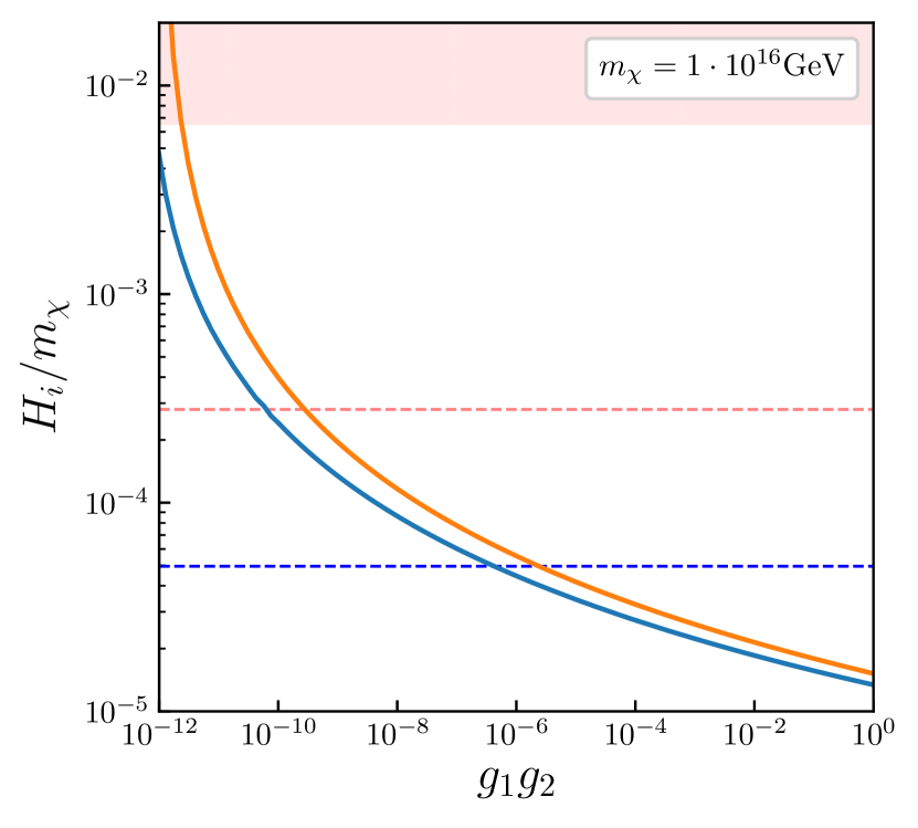
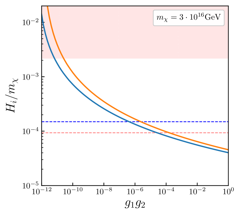
Figure 9: Plot of the critical Hubble rate at the end of inflation as a function of the product of the couplings, for a dark matter mass of $10^{16}\mathrm{GeV}$ (left) and $3\cdot 10^{16}\mathrm{GeV}$ (right). The blue (orange) curve indicates a mediator mass of $1.9\,m_{\chi}$ $(1.0\,m_{\chi})$. The red area at the top is excluded by the currently observed bound for the tensor-to-scalar ratio in the CMB. Additionally, the projected sensitivity of CMB experiments is shown as the dashed red line. Furthermore, the critical Hubble rate of Garny:2015sjg is indicated by the blue dashed line.

4 Results

We have solved the integral (19) numerically. If we use the simplified reheating scenario and a fixed value of the dark matter mass $m_{\chi}$, the resulting abundance $X_{\mathrm{f}}$ depends only on the Hubble rate $H_{i}$ after inflation (which sets the reheating temperature), and the product of the two involved couplings. In principle, there is also a light dependence on the mediator mass $m_{\mathrm{M}}$, however as one observes, varying the mediator mass shows only little effect on the final abundance, especially for larger values of the couplings. Our results are displayed in figure 9. There, we varied the couplings $g_{1}g_{2}$ over a broad range, and determined the value of $H_{i}$ needed to produce the critical dark matter relic abundance $X_{\mathrm{f}}^{\mathrm{crit.}}$, eq. (24).

One observes that for very small couplings, values for the Hubble rate that exceed the current CMB bounds Akrami:2018odb are needed in order to produce the right amount of dark matter. The bounds are more strict for lower mediator masses. Likewise, the critical Hubble rate changes for less than an order of magnitude for a wide range of coupling strengths, roughly from $g_{1}g_{2}=10^{-8}$ to $g_{1}g_{2}=1$.

Moreover, one observes that for values of $g_{1}g_{2}$ greater than $10^{-6}$, the production of dark matter via the stringy operators largely dominates the graviton exchange presented in ref. Garny:2015sjg ; Garny:2017kha and therefore neglecting this gravitational channel is a good assumption. For lighter dark matter masses it is impossible to get near the CMB bound, even the projected ones, without encountering overproduction by graviton exchange first. However, starting from $m_{\chi}\sim 3\cdot 10^{16}\mathrm{GeV}$, our approach becomes sensitive to at least the projected CMB bound in ranges for the stringy couplings for which graviton exchange can still be safely neglected. We also observe that for any value of the couplings, our Hubble rate lies in ranges where – given the DM mass – gravitational production Chung:2001cb can be neglected.

5 Conclusions

We have shown that generic string constructions can accommodate a candidate for dark matter. Opposed to other studies of dark matter in string theory (cf. Chowdhury:2018tzw ; Bhattacharyya:2018evo ; Bernal:2018qlk ), we focused on the dark matter candidate, as e.g. in Halverson:2016nfq ; Halverson:2018olu . Specifically, the dark matter candidate is a heavy string state with no charge under the Standard Model gauge group and a mass at or above the GUT scale. It is stabilized against decay by stringy selection rules, closely related to the topological property of a non-trivial fundamental group $\pi_{1}$ of the compactification space. Because of its high mass, the dark matter particle never attains thermal equilibrium, and therefore it must be produced by freeze-in rather than freeze-out. We find that generically, the dark matter candidate interacts with the thermal bath only via gravity, and by the exchange of heavy mediators arising in the massive string spectrum. For not too small string couplings the latter ones dominate over graviton exchange.

For definiteness, we considered an explicit model in heterotic orbifolds, but we believe that our results carry over very well to many other string constructions, for example in Calabi–Yau constructions with freely-acting Wilson lines Braun:2005nv ; Anderson:2011ns ; Anderson:2014hia . In our setup, we chose a small-radius limit, where winding strings are the lightest extra states, in order to identify the stringy selection rules. There exists a $T$-dual large-radius picture where the winding states are exchanged by Kaluza–Klein excitations. In our picture, the dark matter candidate is a string with winding around a particular non-contractible cycle on the orbifold, thereby ensuring its stability. An analysis on the level of the orbifold space group reveals that this winding state can couple to the Standard Model – apart from gravity – via the exchange of heavy winding strings that are SM singlets. Going to an $\mathcal{N}=1$ supersymmetric field theory, we identified the relevant terms for $2\rightarrow 2$ production of the heavy dark matter candidate from the Kähler potential and the superpotential. We find that in order to obtain the correct dark matter relic density, one needs values for the Hubble rate at the end of inflation that range up to $10^{12}$ GeV, if the string coupling is perturbative. This way, one is able to constrain the allowed parameter space of the model by bounds on the tensor-to-scalar ratio in the CMB.

We observe that our results generalize very well to generic string models: The most prominent influence comes only from the mass of the dark matter candidate itself, which is constrained to lie around the GUT scale. Other model-dependent parameters, such as the mass of the mediator contribute only at subleading order. Furthermore, the required Hubble rate after inflation remains within the same order of magnitude for the entire sensible range of string couplings. Finally, we observe that adding vectorlike matter that is charged under the SM and contributes to the production of dark matter, changes the critical final abundance only by a small amount, and leaves the required Hubble rate invariant up to the percent level.

Acknowledgements.

This work was supported by the Deutsche Forschungsgemeinschaft (SFB1258). We would like to thank Mathias Garny and Kai Urban for useful discussions.

Appendix A An explicit realization in string theory

We consider the $\mathrm{E}_{8}\times\mathrm{E}_{8}$ heterotic string theory compactified on the $\mathbbm{Z}_{2}\times\mathbbm{Z}_{2}$-5-1 orbifold geometry Dixon:1985jw ; Dixon:1986jc ; Ibanez:1986tp , see also refs. Forste:2006wq ; Donagi:2008xy ; Fischer:2012qj and refs. Blaszczyk:2009in ; Olguin-Trejo:2018wpw for MSSM-like string models based on this orbifold geometry. This orbifold geometry can be constructed in three steps. First, one defines a factorized six-torus $\mathbb{T}^{6}=\mathbb{T}^{2}\times\mathbb{T}^{2}\times\mathbb{T}^{2}$ via a six-dimensional lattice that is spanned by six basis vectors $e_{i}$, $i=1,\ldots,6$. Then, this six-torus is orbifolded by $\mathbbm{Z}_{2}\times\mathbbm{Z}_{2}$ rotations $\theta\mathrel{\widehat{=}}(0,\nicefrac{{1}}{{2}},-\nicefrac{{1}}{{2}})$ and $\omega\mathrel{\widehat{=}}(\nicefrac{{1}}{{2}},0,-\nicefrac{{1}}{{2}})$, indicating the rotation angles in units of $2\pi$ in the three complex coordinates corresponding to the three two-tori $\mathbb{T}^{2}$. By doing so, one obtains the $\mathbbm{Z}_{2}\times\mathbbm{Z}_{2}$-1-1 orbifold geometry. Finally, one defines the shift

$$\tau~{}=~{}\frac{1}{2}\left(e_{2}+e_{4}+e_{6}\right)\;.$$ (27)

The resulting six-torus $\mathbb{T}^{6}$ spanned by $e_{1},\ldots,e_{5}$ and $\tau$ is non-factorizable. It turns out that $\tau$ acts freely on the $\mathbbm{Z}_{2}\times\mathbbm{Z}_{2}$-1-1 orbifold, i.e. there is no point on the $\mathbbm{Z}_{2}\times\mathbbm{Z}_{2}$-1-1 orbifold that is invariant under a shift by $\tau$. Hence, $\tau$ is called freely-acting. By modding out the $\mathbbm{Z}_{2}\times\mathbbm{Z}_{2}$-1-1 orbifold by $\tau$, one obtains the $\mathbbm{Z}_{2}\times\mathbbm{Z}_{2}$-5-1 orbifold geometry.

A.1 Strings on orbifolds

Closed strings on orbifolds are characterized by their boundary conditions that specify which transformation is needed such that the string is closed. In more detail, for a string (i.e. a worldsheet boson) $X(\sigma_{0},\sigma_{1})$ as a function of worldsheet time and space coordinates $\sigma_{0}$ and $\sigma_{1}\in[0,1]$ the boundary condition reads

$$X(\sigma_{0},\sigma_{1}+1)~{}=~{}\theta^{k}\,\omega^{\ell}\,X(\sigma_{0},\sigma_{1})+n_{i}\,e_{i}+n_{\tau}\,\tau\quad\Leftrightarrow\quad g~{}=~{}(\theta^{k}\,\omega^{\ell},n_{i}\,e_{i}+n_{\tau}\,\tau)~{}\in~{}S\;,$$ (28)

where $k,\ell\in\{0,1\}$, $n_{i}\in\mathbbm{Z}$, $n_{\tau}\in\{0,1\}$ and summation over $i=1,\ldots,6$ is implied. Strings with $k\neq 0$ or $\ell\neq 0$ are called twisted strings, in contrast to the case $k=\ell=0$ which gives rise to so-called untwisted strings. One can encode the boundary condition (28) into group elements $g\in S$ of the so-called space group $S$. Then, $g$ is called the constructing element of the string (28). In more detail, since $X$ and $h\,X$ are identified on the orbifold for all $h\in S$, a string is actually characterized not only by the single constructing element $g\in S$ but by the conjugacy class $[g]=\{h\,g\,h^{-1}~{}|~{}h\in S\}$. If $g\in[g]\subset S$ has a fixed point, i.e. if there is a point $x_{g}$ such that $\theta^{k}\omega^{\ell}x_{g}+n_{i}\,e_{i}+n_{\tau}\,\tau=x_{g}$, the string with constructing element $g$ is localized in the extra dimensions at $x_{g}$. It is important to remark that the freely-acting nature of $\tau$ becomes evident by noticing that constructing elements with fixed points necessarily have $n_{\tau}=0$. Furthermore, strings with boundary conditions $(\mathbbm{1},n_{i}\,e_{i}+n_{\tau}\,\tau)\in S$ live in the orbifold bulk. They are winding strings if $n_{i}\neq 0$ or $n_{\tau}\neq 0$, where the mass of a winding string is proportional to the radius and the winding number of its winding direction, as we will discuss later in appendix A.3. Hence, in general only bulk strings with constructing element $(\mathbbm{1},0)$ are massless.

The $\mathbbm{Z}_{2}\times\mathbbm{Z}_{2}$-5-1 orbifold geometry has the important property of having a cycle that generates a non-trivial fundamental group $\pi_{1}$ Dixon:1986jc and, hence, renders the orbifold geometry non-simply connected. In fact, this cycle is generated by the freely-acting shift $\tau$. The existence of the freely-acting shift has two important consequences for our discussion:

1. There are heavy string modes with constructing elements $(\mathbbm{1},n_{\tau}\tau)\in S$ that wind around the freely-acting $\tau$-direction and

2. There is an exact $\mathbbm{Z}_{4}$ symmetry Ramos-Sanchez:2018edc , where a string with general constructing element eq. (28) carries a discrete charge

   $$Q~{}=~{}n_{\tau}+2(n_{2}+n_{4}+n_{6})\;\;\mathrm{mod}\;\;4\quad\mathrm{such\ that}\quad Q~{}\in~{}[0,1,2,3]\;,$$ (29)

   where $n_{\tau}\in\{0,1\}$ and $n_{2},n_{4},n_{6}\in\mathbbm{Z}$ are the integer winding numbers. It turns out that all massless strings (those from the bulk and those that are localized at orbifold fixed points) have $n_{\tau}=0$ and, therefore, carry even $\mathbbm{Z}_{4}$ charges, while there exist massive strings with odd $\mathbbm{Z}_{4}$ charges.

Consequently, there exists a lightest winding string from the bulk with winding numbers $n_{\tau}=1$ and $n_{i}=0$, i.e. with constructing element $\left(\mathbbm{1},\,\tau\right)$, that has odd $\mathbbm{Z}_{4}$ charge. Hence, it is stable and we can identify it as our dark matter candidate $\Phi_{\mathrm{DM}}$. Its mass partner $\Phi_{\mathrm{DM}}^{\prime}$ has constructing element $\left(\mathbbm{1},\,-\tau\right)$ and therefore $\mathbbm{Z}_{4}$ charge 3.

A.2 String interactions

In order to find the three point couplings allowed by the space group selection rule Hamidi:1986vh ; Dixon:1986qv , one needs to fulfill for each coupling that

$$(\mathbbm{1},0)~{}\in~{}[g_{1}]\cdot[g_{2}]\cdot[g_{3}]\;,$$ (30)

where $[g_{i}]$ denotes the conjugacy class of the constructing element $g_{i}$. The calculation is the same for the Kähler and the superpotential. In the Kähler potential, one looks for terms of the form $\Phi\Phi^{\dagger}V^{(\mathrm{M})}$, where $\Phi^{\dagger}$ has inverted quantum numbers and hence has the inverse constructing element. In the superpotential, one looks for terms of the form $\Phi_{1}\Phi_{2}\Phi_{\mathrm{M}}$, where $\Phi_{2}$ is either the mass partner of $\Phi_{1}$ (for the dark matter particle and the Higgs portal), or it is another field localized appropriately (for the neutrino portal).

In any case, we observe that there exist several winding states with trivial $\mathbbm{Z}_{4}$ charge, most prominently those with $n_{2}+n_{4}+n_{6}=0\;\mathrm{mod}\;2$. These states are particularly interesting candidates for mediators:

1. On the level of space group elements, they couple to both, DM and twisted strings. Let us work out for the coupling of dark matter to the $\theta$-twisted sector (i.e. $k=1$ and $\ell=0$ in eq. (28)).

   • It is evident that $\left(\mathbbm{1},\,\frac{1}{2}(e_{2}-e_{4}-e_{6})\right)\in\left[\left(\mathbbm{1},\,\tau\right)\right]$ and $\left(\mathbbm{1},\,-\frac{1}{2}(e_{2}+e_{4}+e_{6})\right)\in\left[\left(\mathbbm{1},\,-\tau\right)\right]$. Hence, $\left(\mathbbm{1},\,0\right)\in\left[\left(\mathbbm{1},\,\tau\right)\right]\cdot\left[\left(\mathbbm{1},\,-\tau\right)\right]\cdot\left(\mathbbm{1},\,e_{4}+e_{6}\right)$.

   • Similarly, $\left(\mathbbm{1},\,-\tau\right)\left(\theta,\,0\right)\left(\mathbbm{1},\,\tau\right)=\left(\theta,\,-e_{4}-e_{6}\right)\in\left[\left(\theta,\,0\right)\right]$. Hence, $\left(\mathbbm{1},\,0\right)\in\left(\mathbbm{1},\,e_{4}+e_{6}\right)\cdot\left[\left(\theta,\,0\right)\right]\cdot\left[\left(\theta,\,0\right)\right]$.

2. Their local shift is a lattice vector, cf. ref. Blaszczyk:2009in . Hence, these states have $p_{\mathrm{sh}}=0$ and the corresponding couplings are not forbidden by gauge invariance.

It turns out that the construction shown above not only works for the $\theta$-, but also for the $\omega$- and $\theta\omega$-twisted sector. In summary, we have the winding strings $V^{(\mathrm{M})}$ and $\Phi_{\mathrm{M}}$ that mediate between the dark matter strings ($\Phi_{\mathrm{DM}}$ and $\Phi_{\mathrm{DM}}^{\prime}$) and the twisted sector

sector of SM	$\theta$	$\omega$	$\theta\omega$
$g\in S$ of mediator	$\left(\mathbbm{1},\,e_{4}+e_{6}\right)$	$\left(\mathbbm{1},\,e_{2}+e_{6}\right)$	$\left(\mathbbm{1},\,e_{2}+e_{4}\right)$

In the next section, we will discuss the winding strings with constructing elements $\left(\mathbbm{1},\,\tau\right)$ and $\left(\mathbbm{1},\,e_{4}+e_{6}\right)$ in more detail.

A.3 Massive $\mathrm{U}(1)$ gauge bosons from string theory

After the general discussion on the string origin of our dark matter candidate $\Phi_{\mathrm{DM}}$ and of the massive mediators $V^{(\mathrm{M})}$ and $\Phi_{\mathrm{M}}$, we now give more details on their existence and mass.

In heterotic string theory, a general string state is built out of independent right- and left-movers

$$\ket{p_{\mathrm{R}};q}_{\mathrm{R}}\otimes\ket{p_{\mathrm{L}};p_{\mathrm{sh}}}_{\mathrm{L}}\;,$$ (31)

possibly subject to string oscillator excitations. Furthermore, $q$ is the bosonized right-moving $H$-momentum, being

$$q~{}\in~{}\big{\{}\big{(}\underline{\pm 1,0,0,0}\big{)}\;,\;\big{(}\pm\nicefrac{{1}}{{2}},\pm\nicefrac{{1}}{{2}},\pm\nicefrac{{1}}{{2}},\pm\nicefrac{{1}}{{2}}\big{)}\big{\}}\;.$$ (32)

Here, the underline denotes all permutations and the number of plus-signs must be even for half-integer entries. In other words, $q$ is either an $\mathbf{8}_{\mathrm{v}}$ or an $\mathbf{8}_{\mathrm{s}}$ weight vector of $\mathrm{SO}(8)$ that fulfills $q^{2}=1$. Its first entry reflects the four-dimensional space-time chirality of the corresponding string state. In addition, the shifted left-moving momentum $p_{\mathrm{sh}}=p+A\,n$ in eq. (31) is given by the so-called discrete Wilson lines $A$ Ibanez:1986tp and the momentum $p$ that belongs to the sixteen-dimensional $\mathrm{E}_{8}\times\mathrm{E}_{8}$ root lattice. Most important for our discussion are the right- and left-moving momenta, which are given by

$$p_{\mathrm{R}} := \frac{e^{-\mathrm{T}}}{\sqrt{2}}\left(\left(G-B+\frac{1}{2}A^{\mathrm{T}}A\right)\,n-m+A^{\mathrm{T}}p\right)\;,$$ (33a)

$$p_{\mathrm{L}} := \frac{e^{-\mathrm{T}}}{\sqrt{2}}\left(\left(G+B-\frac{1}{2}A^{\mathrm{T}}A\right)\,n+m-A^{\mathrm{T}}p\right)\;,$$ (33b)

using the convention $\alpha^{\prime}=1$, cf. ref. GrootNibbelink:2017usl . Here, similar to the discussion at the beginning of section A, $e$ denotes the geometrical vielbein that defines the $D$-dimensional torus $\mathbb{T}^{D}$ with metric $G:=e^{\mathrm{T}}e$ and $B$ is the anti-symmetric $B$-field. Moreover, $n\in\mathbbm{Z}^{D}$ are the integer winding numbers defined in analogy to eq. (28) by the boundary condition of a bulk string

$$X(\sigma_{0},\sigma_{1}+1)~{}=~{}X(\sigma_{0},\sigma_{1})+e\,n\;,\quad\mathrm{where}\quad e\,n~{}=~{}\frac{1}{\sqrt{2}}\left(p_{\mathrm{R}}+p_{\mathrm{L}}\right)\;,$$ (34)

and $m\in\mathbbm{Z}^{D}$ denote the integer Kaluza–Klein (KK) numbers. Note that the $(2D+16)$-dimensional vectors $(p_{\mathrm{R}},p_{\mathrm{L}},p_{\mathrm{sh}})$ span an even, integer and self-dual lattice with signature $(D,D+16)$, called the Narain lattice. As such, a vector given by eqs. (33) satisfies for example

$$-(p_{\mathrm{R}})^{2}+(p_{\mathrm{L}})^{2}+(p_{\mathrm{sh}})^{2}~{}=~{}2\,m^{\mathrm{T}}n+p^{2}~{}=~{}\mathrm{even}\;,$$ (35)

reflecting the fact that the Narain lattice is even.

A physical string state from eq. (31) is subject to the so-called level-matching condition on right- and left-moving masses, i.e.

$$M_{\mathrm{R}}^{2}~{}=~{}M_{\mathrm{L}}^{2}\;,$$ (36)

where

$$\frac{1}{2}M_{\mathrm{R}}^{2}~{}=~{}(p_{\mathrm{R}})^{2}+q^{2}+2\left(N_{\mathrm{R}}-\frac{1}{2}\right)\quad,\quad\frac{1}{2}M_{\mathrm{L}}^{2}~{}=~{}(p_{\mathrm{L}})^{2}+(p_{\mathrm{sh}})^{2}+2\left(N_{\mathrm{L}}-1\right)\;.$$ (37)

We are interested in winding strings in order to discuss the origin of both, our dark matter candidate $\Phi_{\mathrm{DM}}$ with constructing element $\left(\mathbbm{1},\,\tau\right)\in S$ and the mediators, for example, $V^{(\mathrm{M})}$ and $\Phi_{\mathrm{M}}$ with constructing element $\left(\mathbbm{1},\,e_{4}+e_{6}\right)\in S$. To do so, we can concentrate on three compactified dimensions $D=3$ and focus on the torus directions $e_{2}$, $e_{4}$ and $\tau$, see eq. (27). To keep the discussion short we assume trivial Wilson lines $A_{2}=A_{4}=A_{\tau}=(0^{16})$. Then, we can consider the $\mathbbm{Z}_{2}\times\mathbbm{Z}_{2}$ orbifold of this $\mathbb{T}^{3}$ subsector in order to analyze those winding strings we are mostly interested in.

For the $D=3$ subsector of the $\mathbbm{Z}_{2}\times\mathbbm{Z}_{2}$-5-1 orbifold geometry, the Narain lattice eq. (33) can be parameterized by three radii $R_{2}$, $R_{4}$ and $R_{6}$ for the torus vielbein $e$ and three parameters $b_{1}$, $b_{2}$ and $b_{3}$ for the anti-symmetric $B$-field, i.e.

$$e~{}=~{}\left(\begin{array}[]{ccc}R_{2}&0&\nicefrac{{R_{2}}}{{2}}\\ 0&R_{4}&\nicefrac{{R_{4}}}{{2}}\\ 0&0&\nicefrac{{R_{6}}}{{2}}\end{array}\right)\quad,\quad B~{}=~{}\left(\begin{array}[]{ccc}0&b_{1}&b_{2}\\ -b_{1}&0&b_{3}\\ -b_{2}&-b_{3}&0\end{array}\right)\;.$$ (38)

Thus, the columns of the geometrical vielbein $e$ are given by $e_{2}$, $e_{4}$ and $\tau$, cf. eq. (27). Consequently, eq. (38) has six free parameters (which combine in the six-dimensional $\mathbbm{Z}_{2}\times\mathbbm{Z}_{2}$ orbifold with six additional parameters to three Kähler moduli $T_{i}$ and three complex structure moduli $U_{i}$, $i=1,2,3$).

Let us begin with the discussion on the mediator with constructing element $\left(\mathbbm{1},\,e_{4}+e_{6}\right)$. In terms of the basis $e_{2}$, $e_{4}$ and $\tau$, we use $e_{6}=2\tau-e_{2}-e_{4}$ to write $\left(\mathbbm{1},\,e_{4}+e_{6}\right)=\left(\mathbbm{1},\,2\tau-e_{2}\right)$. Hence, the mediator has winding numbers $n=(-1,0,2)^{\mathrm{T}}$ such that $e\,n=2\tau-e_{2}$. It turns out that there exists a point in moduli space (i.e. with special values for the radii $R_{i}$ and $B$-field components $b_{i}$), where the mediator $\left(\mathbbm{1},\,2\tau-e_{2}\right)$ becomes massless. Thus, we start our discussion at this point in moduli space and, afterwards, move in moduli space to make the mediator massive.

Massless strings must have vanishing right- and left-moving masses eqs. (37), subject to $M_{\mathrm{R}}^{2}=M_{\mathrm{L}}^{2}$. A vanishing right-moving mass implies $p_{\mathrm{R}}=(0^{3})$ and, hence,

$$m~{}=~{}(G-B)\,n\;,\quad\mathrm{using}\quad A_{2}~{}=~{}A_{4}~{}=~{}A_{\tau}=(0^{16})$$ (39)

and $q^{2}=1$ and $N_{\mathrm{R}}=0$ in eq. (37). In this case, $p_{\mathrm{L}}$ is given by $p_{\mathrm{L}}=\sqrt{2}\,e\,n$. Consequently, a vanishing left-moving mass, eq. (37) with $p=(0^{16})$ and $N_{\mathrm{L}}=0$, yields the constraint

$$n^{\mathrm{T}}G\,n~{}=~{}1\quad\Leftrightarrow\quad(R_{4})^{2}+(R_{6})^{2}~{}=~{}1\;,$$ (40)

for our mediator string with winding numbers $n=(-1,0,2)^{\mathrm{T}}$. Note that one can check that this mass condition is identical for all four winding strings in the conjugacy class $[\left(\mathbbm{1},\,2\tau-e_{2}\right)]$, as expected. In order to satisfy the mass condition (40), we choose

$$(R_{4})^{2}~{}=~{}(R_{6})^{2}~{}=~{}\nicefrac{{1}}{{2}}\;.$$ (41)

Next, we have to fix the remaining moduli parameters $b_{i}$ such that the KK numbers $m$ in eq. (39) become integer. In other words, a general winding string $n\neq(0^{3})$ necessarily carries non-trivial KK numbers $m\neq(0^{3})$ in order to satisfy eq. (39) and, hence, level-matching. We find a solution for

$$b_{1}~{}=~{}0\quad,\quad b_{2}~{}=~{}\nicefrac{{1}}{{2}}\quad\mathrm{and}\quad b_{3}=-\nicefrac{{1}}{{4}}\;,$$ (42)

such that $m=(-1,1,0)^{\mathrm{T}}$ satisfies eq. (39). Let us give two import remarks: First, at a generic point in moduli space the total mass squared $M_{\mathrm{R}}^{2}+M_{\mathrm{L}}^{2}$ of the mediator depends on all six free parameters $b_{i}$, $i=1,2,3$, $R_{2}$, $R_{4}$ and $R_{6}$. However, there are special points in moduli space, where the mass is independent of, for example, the compactification radius $R_{2}$: this is the case at $b=\nicefrac{{1}}{{2}}$. Secondly, since $m^{\mathrm{T}}n=1$ and $p=(0^{16})$, the even Narain lattice ensures that $-(p_{\mathrm{R}})^{2}+(p_{\mathrm{L}})^{2}=2$, see eq. (35). Hence, the level-matching condition (36) is satisfied everywhere in moduli space for this string.

Next, we consider the dark matter candidate $\Phi_{\mathrm{DM}}$ with constructing element $\left(\mathbbm{1},\,\tau\right)\in S$. In this case, the corresponding winding numbers are given by $n=(0,0,1)^{\mathrm{T}}$ such that $e\,n=\tau$. Since we are interested in the lightest string state with these winding numbers, we set $N_{\mathrm{R}}=N_{\mathrm{L}}=0$ and $p=(0^{16})$. Note that $p$ defines the representation of $\Phi_{\mathrm{DM}}$ under the four-dimensional gauge group, which originates from $\mathrm{E}_{8}\times\mathrm{E}_{8}$ and is assumed to contain the Standard Model gauge group. Hence, $p=(0^{16})$ renders $\Phi_{\mathrm{DM}}$ a Standard Model singlet. Now, we have to find KK numbers $m\in\mathbbm{Z}^{3}$ such that $m^{\mathrm{T}}n=1$. Then, the Narain condition $-(p_{\mathrm{R}})^{2}+(p_{\mathrm{L}})^{2}=2m^{\mathrm{T}}n=2$ ensures level-matching. Hence, $m=(m_{1},m_{2},1)^{\mathrm{T}}$ with $m_{1}$, $m_{2}\in\mathbbm{Z}$ is the general solution. Now, let us find the lightest dark matter candidate $\Phi_{\mathrm{DM}}$. To do so, we assume eqs. (41) and (42), and compute the total mass squared of $\Phi_{\mathrm{DM}}$ in terms of the free radius $r=(R_{2})^{2}$ and KK numbers $m_{1}$, $m_{2}\in\mathbbm{Z}$,

$$M^{2}(r,m_{1},m_{2}) \propto (p_{\mathrm{R}})^{2}+(p_{\mathrm{L}})^{2}-2$$

$$\propto 18+8m_{1}^{2}+16m_{2}(m_{2}-2)+4m_{1}(4m_{2}-7)+\frac{(1+2m_{1})^{2}}{r}+r\;.$$

Let us constrain the radius $R_{2}$ to $0<R_{2}<1$. In this range, the $\tau$-winding string with minimal mass has KK numbers $m=(0,1,1)^{\mathrm{T}}$: in figure 10 we plot the masses as functions of $r=(R_{2})^{2}$ for various $\tau$-winding strings with KK numbers in the ranges $-5\leq m_{i}\leq 5$ for $i=1,2$ and identify the lightest string.

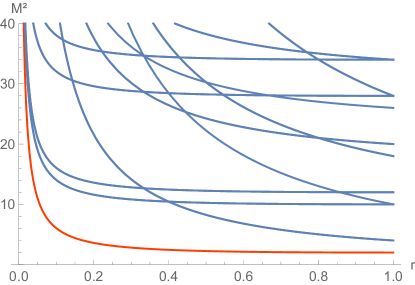
Figure 10: The mass squared $M^{2}$ (in string units $\alpha^{\prime}=1$) of dark matter candidates with constructing element $\left(\mathbbm{1},\,\tau\right)\in S$ and various KK numbers $-5\leq m_{i}\leq 5$ for $i=1,2$ (and $m_{3}=1$) depending on the compactification radius $r=(R_{2})^{2}$. The lightest $\tau$-winding string state (in red) is specified by $n=(0,0,1)^{\mathrm{T}}$ and $m=(0,1,1)^{\mathrm{T}}$. In this figure, the other moduli parameters are set according to eqs. (41) and (42), where the mediator is massless independently of $r=(R_{2})^{2}$. There are other points in moduli space, where the masses of the lightest dark matter candidate and of the mediator are much smaller than 1.

Consequently, we have identified the lightest $\tau$-winding string state, specified by winding and KK numbers

$$n~{}=~{}(0,0,1)^{\mathrm{T}}\quad\mathrm{and}\quad m~{}=~{}(0,1,1)^{\mathrm{T}}\;,$$ (44)

respectively. This massive string is our dark matter candidate $\Phi_{\mathrm{DM}}$. It is a Standard Model singlet, i.e. $p=(0^{16})$, and stable since it carries an odd $\mathbbm{Z}_{4}$ charge $Q=1$, cf. eq. (29). Furthermore, the lightest mediator corresponding to a winding string with constructing element $\left(\mathbbm{1},\,e_{4}+e_{6}\right)\in S$ is characterized by winding and KK numbers

$$n~{}=~{}(-1,0,2)^{\mathrm{T}}\quad\mathrm{and}\quad m~{}=~{}(-1,1,0)^{\mathrm{T}}\;,$$ (45)

respectively. In contrast to the the dark matter candidate, the mediator is uncharged under $\mathbbm{Z}_{4}$, cf. eq. (29). As we have shown, if we keep $b_{2}=\nicefrac{{1}}{{2}}$ fixed, we can independently vary the masses of $\Phi_{\mathrm{DM}}$ and the mediator. Finally, it is important to comment that the mediator corresponds to a $\mathrm{U}(1)$ gauge boson that becomes massless at a specific point in moduli space, given in eqs. (41) and (42). Moreover, using the results of ref. Beye:2014nxa , we know that the massive $\tau$-winding string state is charged under this $\mathrm{U}(1)$. Hence, a Kähler potential of the form eq. (2) must originate from this string construction.

References

- (1) E. W. Kolb and M. S. Turner, The Early Universe, Front. Phys. 69 (1990) 1.
- (2) G. Jungman, M. Kamionkowski and K. Griest, Supersymmetric dark matter, Phys. Rept. 267 (1996) 195 [hep-ph/9506380].
- (3) L. J. Hall, K. Jedamzik, J. March-Russell and S. M. West, Freeze-In Production of FIMP Dark Matter, JHEP 03 (2010) 080 [0911.1120].
- (4) M. Garny, M. Sandora and M. S. Sloth, Planckian Interacting Massive Particles as Dark Matter, Phys. Rev. Lett. 116 (2016) 101302 [1511.03278].
- (5) M. Garny, A. Palessandro, M. Sandora and M. S. Sloth, Theory and Phenomenology of Planckian Interacting Massive Particles as Dark Matter, JCAP 1802 (2018) 027 [1709.09688].
- (6) Ya. I. Kogan and M. Yu. Khlopov, Homotopically stable particles in the superstring theory, Sov. J. Nucl. Phys. 46 (1987) 193.
- (7) S. Ramos-Sánchez and P. K. S. Vaudrevange, Note on the space group selection rule for closed strings on orbifolds, JHEP 01 (2019) 055 [1811.00580].
- (8) T. Banks and M. Dine, Note on discrete gauge anomalies, Phys. Rev. D45 (1992) 1424 [hep-th/9109045].
- (9) H. M. Lee, S. Raby, M. Ratz, G. G. Ross, R. Schieren, K. Schmidt-Hoberg et al., Discrete R symmetries for the MSSM and its singlet extensions, Nucl. Phys. B850 (2011) 1 [1102.3595].
- (10) M. Fischer, M. Ratz, J. Torrado and P. K. S. Vaudrevange, Classification of symmetric toroidal orbifolds, JHEP 01 (2013) 084 [1209.3906].
- (11) L. J. Dixon, V. Kaplunovsky and J. Louis, Moduli dependence of string loop corrections to gauge coupling constants, Nucl. Phys. B355 (1991) 649.
- (12) P. Gondolo and G. Gelmini, Cosmic abundances of stable particles: Improved analysis, Nucl. Phys. B360 (1991) 145.
- (13) J. Edsjo and P. Gondolo, Neutralino relic density including coannihilations, Phys. Rev. D56 (1997) 1879 [hep-ph/9704361].
- (14) G. N. Felder, L. Kofman and A. D. Linde, Instant preheating, Phys. Rev. D59 (1999) 123523 [hep-ph/9812289].
- (15) Planck collaboration, Planck 2018 results. X. Constraints on inflation, 1807.06211.
- (16) J. Errard, S. M. Feeney, H. V. Peiris and A. H. Jaffe, Robust forecasts on fundamental physics from the foreground-obscured, gravitationally-lensed CMB polarization, JCAP 1603 (2016) 052 [1509.06770].
- (17) Planck collaboration, Planck 2018 results. VI. Cosmological parameters, 1807.06209.
- (18) D. J. H. Chung, P. Crotty, E. W. Kolb and A. Riotto, On the Gravitational Production of Superheavy Dark Matter, Phys. Rev. D64 (2001) 043503 [hep-ph/0104100].
- (19) D. Chowdhury, E. Dudas, M. Dutra and Y. Mambrini, Moduli Portal Dark Matter, Phys. Rev. D99 (2019) 095028 [1811.01947].
- (20) G. Bhattacharyya, M. Dutra, Y. Mambrini and M. Pierre, Freezing-in dark matter through a heavy invisible Z’, Phys. Rev. D98 (2018) 035038 [1806.00016].
- (21) N. Bernal, M. Dutra, Y. Mambrini, K. Olive, M. Peloso and M. Pierre, Spin-2 Portal Dark Matter, Phys. Rev. D97 (2018) 115020 [1803.01866].
- (22) J. Halverson, B. D. Nelson and F. Ruehle, String Theory and the Dark Glueball Problem, Phys. Rev. D95 (2017) 043527 [1609.02151].
- (23) J. Halverson, B. D. Nelson, F. Ruehle and G. Salinas, Dark Glueballs and their Ultralight Axions, Phys. Rev. D98 (2018) 043502 [1805.06011].
- (24) V. Braun, Y.-H. He, B. A. Ovrut and T. Pantev, The Exact MSSM spectrum from string theory, JHEP 05 (2006) 043 [hep-th/0512177].
- (25) L. B. Anderson, J. Gray, A. Lukas and E. Palti, Two Hundred Heterotic Standard Models on Smooth Calabi-Yau Threefolds, Phys. Rev. D84 (2011) 106005 [1106.4804].
- (26) L. B. Anderson, A. Constantin, S.-J. Lee and A. Lukas, Hypercharge Flux in Heterotic Compactifications, Phys. Rev. D91 (2015) 046008 [1411.0034].
- (27) L. J. Dixon, J. A. Harvey, C. Vafa and E. Witten, Strings on Orbifolds, Nucl. Phys. B261 (1985) 678.
- (28) L. J. Dixon, J. A. Harvey, C. Vafa and E. Witten, Strings on Orbifolds. 2., Nucl. Phys. B274 (1986) 285.
- (29) L. E. Ibáñez, H. P. Nilles and F. Quevedo, Orbifolds and Wilson Lines, Phys. Lett. B187 (1987) 25.
- (30) S. Förste, T. Kobayashi, H. Ohki and K.-j. Takahashi, Non-Factorisable Heterotic Orbifold Models and Yukawa Couplings, JHEP 03 (2007) 011 [hep-th/0612044].
- (31) R. Donagi and K. Wendland, On orbifolds and free fermion constructions, J. Geom. Phys. 59 (2009) 942 [0809.0330].
- (32) M. Blaszczyk, S. Groot Nibbelink, M. Ratz, F. Ruehle, M. Trapletti and P. K. S. Vaudrevange, A standard model, Phys. Lett. B683 (2010) 340 [0911.4905].
- (33) Y. Olguín-Trejo, R. Pérez-Martínez and S. Ramos-Sánchez, Charting the flavor landscape of MSSM-like Abelian heterotic orbifolds, Phys. Rev. D98 (2018) 106020 [1808.06622].
- (34) S. Hamidi and C. Vafa, Interactions on Orbifolds, Nucl. Phys. B279 (1987) 465.
- (35) L. J. Dixon, D. Friedan, E. J. Martinec and S. H. Shenker, The Conformal Field Theory of Orbifolds, Nucl. Phys. B282 (1987) 13.
- (36) S. Groot Nibbelink and P. K. S. Vaudrevange, T-duality orbifolds of heterotic Narain compactifications, JHEP 04 (2017) 030 [1703.05323].
- (37) F. Beye, T. Kobayashi and S. Kuwakino, Gauge Origin of Discrete Flavor Symmetries in Heterotic Orbifolds, Phys. Lett. B736 (2014) 433 [1406.4660].