Trapezoidal methods for fractional differential equations: theoretical and computational aspects

Abstract

The paper describes different approaches to generalize the trapezoidal method to fractional differential equations. We analyze the main theoretical properties and we discuss computational aspects to implement efficient algorithms. Numerical experiments are provided to illustrate potential and limitations of the different methods under investigation.

Keywords: fractional differential equations, multistep methods, trapezoidal method, convergence, stability, computational aspects.

1 Introduction

It is nowadays well established that several real–life phenomena are better described by fractional differential equations (FDEs), where the term fractional, used for historical reasons, refers to derivative operators of any real positive order. Applications of FDEs are commonly found in bioengineering, chemistry, control theory, electronic circuit theory, mechanics, physics, seismology, signal processing and so on (e.g., [3, 7, 5, 33, 22, 41, 50]). We refer to [40] for an historical perspective on fractional calculus.

As a consequence of the growing interest for fractional order models, the analysis and the development of numerical methods for FDEs and partial differential equations with time or space fractional derivatives have become an active area of research (see, for instance, [4, 18, 17, 13, 25, 26, 32, 35, 38, 44, 45, 47, 48, 46, 53, 54]).

Some of the methods for FDEs are directly derived from methods for integral equations; this is the case, for instance, of product integration (PI) rules. A completely different approach, named as fractional linear multistep methods (FLMMs) [38], has instead been specifically tailored to provide a solid theoretical background for the numerical treatment of FDEs.

Interestingly, these two approaches (PI and FLMM) lead to the same methods when the fractional order $\alpha$ converges to the nearest integer; indeed, different methods for FDEs are often generalizations of the same corresponding method for ordinary differential equations (ODEs).

Some important differences are however observed in the pure fractional case. For instance, the PI and FLMM generalizations of the implicit Euler method behave in a different way when applied to problems with discontinuous right–hand side [10, 11, 12] and only the method devised in the framework of FLMMs succeeds in stabilizing the solution on the switching surface, as expected from theoretical considerations, without generating unwanted spurious oscillations [24].

The presence of distinguishing characteristics in methods for FDEs developed from the same method for ODEs deserves to be more thoroughly investigated. Some differences are of theoretical interest (convergence, stability, etc.); nevertheless, the two approaches also present distinctive features of computational nature that affect the efficiency of the solution process.

The main aim of this paper is to describe and compare some methods for FDEs, highlight strengths and weaknesses and investigate the circumstances under which a certain method is preferable to some others.

The analysis will be confined to those PI rules and FLMMs that generalize, in some respects, the implicit second–order trapezoidal rule. This $A$–stable one–step method has the smallest possible error constant [34] and is appreciated since provides a satisfactory balance between accuracy, stability properties and computational complexity. Our interest is in exploring when these strengths are inherited by the corresponding methods for FDEs.

There are also some more specific motivations for restricting the attention to second–order methods: a) PI rules very seldom converge with an order equal or greater than 2; b) the implementation of higher order FLMMs is usually computationally demanding; c) as for multistep methods for ODEs, order 2 represents a barrier for stability.

Despite this apparently limited extent, we will however be able to include in our analysis a sufficiently large number of methods.

The choice of focusing on implicit methods is also motivated by the fact that they have been so far very seldom investigated (very often, implicit methods are taken into account in the framework of predictor–corrector algorithms in which the implicit scheme is actually implemented as an explicit one) and explicit methods are unduly preferred in most of the works on FDEs, regardless of stability issues which discourage their use.

The paper is organized as follows. In Section 2 we present some basic definitions and properties concerning FDEs. Section 3 is devoted to describe PI rules and discuss different implementations on uniform and graded grids. In Section 4 we present FLMMs and we describe three different generalizations of the implicit trapezoidal rule; the use of an effective formula for the evaluation of the weights is also proposed. In Section 5 linear stability is investigated and some implementation details are discussed in Section 6. Finally, in Section 7 the results of some numerical tests are presented to compare the methods under investigation and some concluding remarks are presented at the end of the paper.

2 Fractional differential equations

Let us consider the initial value problem for a system of FDEs in the form

$$\left\{\begin{array}[]{l}{}^{C}D^{\alpha}_{t_{0}}y(t)=f(t,y(t))\\ y^{(k)}(t_{0})=y_{0,k},\quad k=0,\dots m-1\end{array}\right.,$$ (1)

where $m=\left\lceil\alpha\right\rceil$ is the smallest integer such that $m>\alpha$, $f:[t_{0},T]\times\mathbb{R}^{q}\to\mathbb{R}^{q}$ is assumed to be sufficiently smooth, $y:[t_{0},T]\to\mathbb{R}^{q}$ is the unknown solution and $y^{(k)}$ denotes classical derivative of integer order $k$.

The fractional derivative operator ${}^{C}D^{\alpha}_{t_{0}}$ is introduced in this paper according to the Caputo’s definition [14, 42, 49]

$${}^{C}D^{\alpha}_{t_{0}}y(t)=I_{t_{0}}^{m-\alpha}y^{(m)}(t),$$

with $I_{t_{0}}^{\beta}$ the Riemann–Liouville (RL) integral of order $\beta$ on the interval $[t_{0},t]$

$$I_{t_{0}}^{\beta}g(t)=\frac{1}{\Gamma(\beta)}\int_{t_{0}}^{t}(t-s)^{\beta-1}g(s)ds.$$ (2)

A classical result in fractional calculus [14] allows to compute, for any $\alpha\in\mathbb{R}$, the RL integral of the power function as

$$I_{t_{0}}^{\alpha}(t-t_{0})^{\nu}=\frac{\Gamma(\nu+1)}{\Gamma(\alpha+\nu+1)}(t-t_{0})^{\alpha+\nu},\quad\nu>-1,\quad t\geq t_{0}.$$ (3)

It is a well known result that (1) can be equivalently written in terms of the integral equation

$$y(t)=T_{m-1}(t)+I_{t_{0}}^{\alpha}f(t,y(t)),$$ (4)

where $T_{m-1}(t)$ is the Taylor expansion of $y(t)$ centered at $t_{0}$

$$T_{m-1}(t)=\sum_{k=0}^{m-1}\frac{(t-t_{0})^{k}}{k!}y_{0}^{(k)}.$$

One of the major difficulties in the treatment of FDEs derives from the lack of smoothness of the true solution on the whole interval of integration. Indeed, as proved in [36], the true solution of (1) possesses an expansion in mixed (integer and real) powers of the form

$$y(t)=T_{m-1}(t)+\!\!\sum_{\nu\in{\cal A}_{p,m}}\!\!(t-t_{0})^{\nu}Y_{\nu}+{\cal O}\bigl{(}(t-t_{0})^{p}\bigr{)},\quad t\to t_{0},$$ (5)

with $p>m$, ${\cal A}_{p,m}={\cal A}_{p}-\bigl{\{}0,\dots,m-1\bigr{\}}$ and

$${\cal A}_{p}=\bigl{\{}\nu\in\mathbb{R}\,|\,\nu=i+j\alpha,\,i,j\in\mathbb{N},\,\nu<p\bigr{\}},$$

with the consequence that the derivatives of $y(t)$ are unbounded at $t_{0}$.

3 Product integration rules

The main idea behind PI rules [52] is to evaluate the integral in (4) by approximating the vector field $f$ with suitable polynomials. For the integer–order case this is the way in which Adams multistep methods are devised.

To generalize the $1$–step trapezoidal rule consider a (not necessarily uniform) grid $\bigl{\{}t_{0},t_{1},\dots,t_{N}\bigr{\}}$ on the whole interval of integration $[t_{0},T]$ and, in the piecewise decomposition of (4)

$$y(t)=T_{m-1}(t)+\frac{1}{\Gamma(\alpha)}\sum_{j=0}^{n-1}\int_{t_{j}}^{t_{j+1}}(t-s)^{\alpha-1}f(s,y(s))ds,\quad t\geq t_{n},$$

replace $f$ in each subinterval by the first–degree polynomial interpolant

$$p_{j}(s)=f_{j+1}+\frac{s-t_{j+1}}{h_{j}}\bigl{(}f_{j+1}-f_{j}\bigr{)},\quad s\in[t_{j},t_{j+1}],$$

where $h_{j}=t_{j+1}-t_{j}$, $f_{j}=f(t_{j},y_{j})$ and $y_{j}$ is the numerical approximation to the solution $y(t_{j})$. After exactly solving the integrals

$$\frac{1}{\Gamma(\alpha)}\int_{t_{j}}^{t_{j+1}}(t_{n}-s)^{\alpha-1}ds = I_{n,j}^{(0)}-I_{n,j+1}^{(0)},$$

$$\frac{1}{\Gamma(\alpha)}\int_{t_{j}}^{t_{j+1}}(t_{n}-s)^{\alpha-1}\frac{(s-t_{j+1})}{h_{j}}ds = \frac{I_{n,j}^{(1)}}{h_{j}}-I_{n,j}^{(0)}-\frac{I_{n,j+1}^{(1)}}{h_{j}},$$

where, for shortness, we denoted

$$I_{n,j}^{(k)}=\frac{1}{\Gamma(\alpha)}\int_{t_{j}}^{t_{n}}(t_{n}-s)^{\alpha-1}(s-t_{j})^{k}ds=\frac{(t_{n}-t_{j})^{\alpha+k}}{\Gamma(\alpha+k+1)},$$

it is elementary, after a simple change of the summation index, to obtain the numerical approximation of the solution $y(t)$ at $t=t_{n}$ as

$$y_{n}=T_{m-1}(t_{n})+w_{n}f_{0}+\sum_{j=1}^{n}b_{n,j}f_{j},$$ (6)

where

$$\left\{\begin{array}[]{l}\displaystyle w_{n}=I_{n,0}^{(0)}-\frac{I_{n,0}^{(1)}}{h_{0}}+\frac{I_{n,1}^{(1)}}{h_{0}},\\ \displaystyle b_{n,j}=\frac{I_{n,j-1}^{(1)}-I_{n,j}^{(1)}}{h_{j-1}}-\frac{I_{n,j}^{(1)}-I_{n,j+1}^{(1)}}{h_{j}},\quad j=1,\dots,n-1,\quad b_{n,n}=\frac{I_{n,n-1}^{(1)}}{h_{n-1}}.\\ \end{array}\right.$$

According to the analysis presented in [6], this scheme is convergent of second order whenever the true solution is assumed sufficiently smooth. Unfortunately, this is a rather optimistic result compared to the expansion (5) of $y(t)$: due to the presence of unbounded derivatives at $t_{0}$ the convergence rate of (6) is actually lower than the theoretical value $2$, as it can be formally stated by a direct application of the main result by Dixon in [19].

Theorem 1.

Let $f$ be Lipschitz continuous with respect to the second variable and $y_{n}$ the numerical approximation obtained by applying the PI trapezoidal rule (6) on the interval $[t_{0},T]$. There exists a constant $C=C(T-t_{0})$, which does not depend on $h$, such that

$$\left\|y(t_{n})-y_{n}\right\|\leq C\bigl{(}t_{n}^{\alpha-1}h^{1+\alpha}+h^{2}\bigr{)},\quad h=\max_{j=0,\dots,n-1}h_{j}.$$

Unless very restrictive (and usually unrealistic) assumptions are made to ensure the smoothness of $f(t,y(t))$ also at the left endpoint of $[t_{0},T]$, the rate by which the error reduces to $0$ is therefore, away from $t_{0}$, proportional to $h^{1+\alpha}$ when $0<\alpha<1$. The same drop in the convergence order occurs also when higher degree polynomials are employed; for this reason PI rules of higher order are never taken into account for FDEs when $0<\alpha<1$. When $\alpha>1$ order $2$ of convergence is instead obtained.

3.1 Uniform meshes

Using (6) on uniform grids $t_{n}=t_{0}+nh$, with $h>0$ a constant step–size, offers some advantages of computational type. The evaluation of the weights is indeed less expensive and just involves the computation of real powers of integer numbers. Furthermore, (6) presents a convolution structure, in which each weight $b_{n,j}$ depends just on $n-j$, and it can be simplified as

$$y(t_{n})=T_{m-1}(t_{n})+\frac{h^{\alpha}}{\Gamma(\alpha+2)}\left(\tilde{w}_{n}f_{0}+\sum_{j=1}^{n}\tilde{b}_{n-j}f_{j}\right),$$ (7)

where now

$$\left\{\begin{array}[]{l}\tilde{w}_{n}=(\alpha+1-n)n^{\alpha}+(n-1)^{\alpha+1}\\ \tilde{b}_{0}=1,\quad\tilde{b}_{n}=(n-1)^{\alpha+1}-2n^{\alpha+1}+(n+1)^{\alpha+1},\quad n=1,2,\dots\\ \end{array}\right..$$

Formulation (7) of the trapezoidal PI rule is well–known since it is a building component of a widely used predictor–corrector algorithm [18].

The main advantage of the convolution structure is however that (7) can be implemented in a fast way by means of FFT algorithms [28].

3.2 Graded meshes

Unlike FLMMs, PI rules can be implemented on non uniform grids, with the aim of overcoming the order reduction stated in Theorem 1. This issue has been investigated, in the context of weakly singular integral equations, by several authors [1, 9] and graded grids are highly praised to this purpose.

By clustering the grid–points at the left boundary of the integration interval, graded grids are able to cope with the lack of regularity and counteract the inefficiency of polynomials to satisfactorily approximate real powers.

A graded mesh on the interval $[t_{0},T]$ is defined according to

$$t_{n}=t_{0}+\left(\frac{n}{N}\right)^{r}(T-t_{0}),\quad n=0,1,\dots,N,$$

where $r>1$ is a suitable grading exponent. After denoting $h_{0}=t_{1}-t_{0}=(T-t_{0})/{N^{r}}$ and observing that $h_{j}=t_{j+1}-t_{j}=h_{0}\bigl{(}(j+1)^{r}-j^{r}\bigr{)}$, a simple manipulation allows to reformulate (6) according to

$$y(t_{n})=T_{m-1}(t_{n})+\frac{h_{0}^{\alpha}}{\Gamma(\alpha+2)}\left(\hat{w}_{n}f_{0}+\sum_{j=1}^{n}\hat{b}_{n,j}f_{j}\right),$$

where

$$\left\{\begin{array}[]{l}\displaystyle\hat{w}_{n}=(n^{r}-1)^{\alpha+1}-n^{r\alpha}(n^{r}-\alpha-1),\\ \displaystyle\hat{b}_{n,j}=\phi_{n,j}(\alpha,r)-\phi_{n,j+1}(\alpha,r),\quad j=1,\dots,n-1,\quad\hat{b}_{n,n}=(n^{r}-(n-1)^{r})^{\alpha}\\ \end{array}\right.$$

and

$$\phi_{n,j}(\alpha,r)=\frac{(n^{r}-(j-1)^{r})^{(\alpha+1)}-(n^{r}-j^{r})^{(\alpha+1)}}{j^{r}-(j-1)^{r}}.$$

The following result [1, 2] on the second order convergence of graded grids for linear FDEs can be readily extended to more general equations.

Theorem 2.

Let $f(t,y(t))=K(t)y(t)$, $K\in{\cal C}^{2}([t_{0},T])$. For $r=2/\alpha$ it is

$$\left\|y(t_{n})-y_{n}\right\|\leq C_{\alpha}h^{2},\quad h=\!\!\!\!\max_{j=0,\dots,n-1}\!\!\!\!h_{j}=h_{n-1}.$$

The use of PI rules on nonuniform grids is more demanding; not only the weights must be recomputed at each step but, since the absence of a convolution structure, it is not possible to employ fast algorithms. By means of some numerical experiments we will verify, at the end of the paper, whether or not this further amount of computation is, in some way, balanced by the enhancement in the accuracy.

4 Fractional linear multistep methods

In the pioneering work on discretized fractional calculus [38], Lubich proposed an elegant and effective strategy for classical linear multistep methods (LMMs) originally devised for integer–order ODEs.

Although the potentials of FLMMs have been recognized in several papers (see, for instance, the review article by Gorenflo [27]), their use for practical computation has not captured so far widespread attention, perhaps due to some difficulties in explicitly formulating FLMMs.

The key aspect in FLMMs is the approximation of the RL integral (2) by means of the convolution quadrature

$$I_{h}^{\beta}g(t_{n})=h^{\beta}\sum_{j=0}^{n}\omega_{n-j}g(t_{j})+h^{\beta}\sum_{j=0}^{s}w_{n,j}g(t_{j})$$ (8)

on uniform grids $t_{n}=t_{0}+nh$, $h>0$, and where convolution and starting quadrature weights $\omega_{n}$ and $w_{n,j}$ do not depend on $h$.

Starting weights $w_{n,j}$ play an important role, especially in the first part of the integration interval, in order to cope with the possibly singular character of the integrand function at $t_{0}$; we will discuss the problem of their evaluation later on.

Convolution quadrature weights $\omega_{n}$ are the main components of the quadrature rule and characterize the specific FLMM. They are obtained starting from any LMM for ODEs

$$\sum_{j=0}^{k}\rho_{j}y_{n-j}=\sum_{j=0}^{k}\sigma_{j}f(t_{n-j},y_{n-j}),$$

being $\rho(z)=\rho_{0}z^{k}+\rho_{1}z^{k-1}+\dots+\rho_{k}$ and $\sigma(z)=\sigma_{0}z^{k}+\sigma_{1}z^{k-1}+\dots+\sigma_{k}$ the characteristic polynomials. As shown in [51], LMMs can be equivalently reformulated as (8) (but with $\beta=1$ for ODEs) with weights $\omega_{n}$ obtained as the coefficients of the formal power series (FPS)

$$\omega(\xi)=\sum_{n=0}^{\infty}\omega_{n}\xi^{n},\quad\omega(\xi)=\frac{\sigma(1/\xi)}{\rho(1/\xi)}$$

and the function $\omega(\xi)$ goes therefore under the name of generating function of the LMM. The idea proposed in [38] is to generate a quadrature rule for fractional problems (1) by evaluating the convolution weights as the coefficients in the FPS of the fractional–order power of the generating function

$$\omega_{\beta}(\xi)=\sum_{n=0}^{\infty}\omega_{n}\xi^{n},\quad\omega_{\beta}(\xi)=\left(\frac{\sigma(1/\xi)}{\rho(1/\xi)}\right)^{\beta}.$$ (9)

Methods of this kind, named as FLMMs, when applied to (1) read as

$$y_{n}=T_{m-1}(t_{n})+h^{\alpha}\sum_{j=0}^{s}w_{n,j}f_{j}+h^{\alpha}\sum_{j=0}^{n}\omega_{n-j}f_{j}$$ (10)

and their convergence properties are stated in the following result [37, 38].

Theorem 3.

Let $(\rho,\sigma)$ be a stable and consistent of order $p$ implicit LMM with the zeros of $\sigma(\xi)$ having absolute value $\leq 1$. The FLMM (10) is convergent of order $p$.

One of the major difficulties in FLMMs (10) is in evaluating the weights $\omega_{n}$ as the coefficients in the FPS (9). Although some sophisticated algorithms are available for manipulating FPS [31], for most of the methods an efficient tool is the J.C.P. Miller formula stated by the following theorem [30, Theorem 1.6c].

Theorem 4.

Let $\varphi(\xi)=1+\sum_{n=1}^{\infty}a_{n}\xi^{n}$ be a FPS. Then for any $\beta\in\mathbb{C}$,

$$\bigl{(}\varphi(\xi)\bigr{)}^{\beta}=\sum_{n=0}^{\infty}v_{n}^{(\beta)}\xi^{n},$$

where coefficients $v_{n}^{(\beta)}$ can be recursively evaluated as

$$v_{0}^{(\beta)}=1,\quad v_{n}^{(\beta)}=\sum_{j=1}^{n}\left(\frac{(\beta+1)j}{n}-1\right)a_{j}v^{(\beta)}_{n-j}.$$

The Miller formula allows to evaluate, in the most general case, the first $N$ coefficients of $\bigl{(}\varphi(\xi)\bigr{)}^{\beta}$ with a number of operations proportional to $N^{2}$. In most cases of practical interest, this computational effort is actually reduced by an order of magnitude. This is the case of the evaluation of the coefficients $\bigl{\{}\omega_{n}^{(\beta)}\bigr{\}}_{n\in\mathbb{N}}$ in the FPS of $(1\pm\xi)^{\beta}$; indeed, since $a_{1}=\pm 1$ and $a_{2}=a_{3}=\dots=0$, it is elementary to see that the application of Theorem 4 leads to

$$\omega_{0}^{(\beta)}=1,\quad\omega_{n}^{(\beta)}=\pm\left(\frac{\beta+1}{n}-1\right)\omega_{n-1},$$ (11)

involving just $2N$ multiplications and $N$ additions.

4.1 Fractional trapezoidal rule

In order to generalize to FDEs the classical trapezoidal rule, let us first consider its classical formulation for ODEs

$$y_{n+1}-y_{n}=\frac{h}{2}\bigl{(}f_{n}+f_{n+1}\bigr{)},$$ (12)

with characteristic polynomials $\rho(z)=z-1$ and $\sigma(z)=(z+1)/2$ and generating function

$$\omega(\xi)=\frac{\sigma(1/\xi)}{\rho(1/\xi)}=\frac{(1+\xi)}{2(1-\xi)}=\frac{1}{2}\left(1+2\sum_{n=1}^{\infty}\xi^{n}\right).$$

To practically compute the first $N$ weights in the FPS of $\bigl{(}\omega(\xi)\bigr{)}^{\alpha}$ we advise against the direct application of the Miller formula to the infinite series in $\omega(\xi)$ since it would involve a number of operations proportional to $N^{2}$. It is instead preferable to first apply twice Theorem 4 to $\bigl{(}1+\xi\bigr{)}^{\alpha}$ and $\bigl{(}1-\xi\bigr{)}^{-\alpha}$, by means of (11), and hence evaluate the coefficient of their product by an FFT algorithm, with a number of operations proportional to $3N\log_{2}4N$ when $N$ is a power of $2$ [31]. This last task can be efficiently performed by means of the very few lines of Matlab code

x = fft([omega1,zeros(size(omega1))]) ;
y = fft([omega2,zeros(size(omega2))]) ;
omega = ifft(x.*y) ; omega = omega(1:N) ;

where omega1 and omega2 are the row arrays with coefficients of $\bigl{(}1+\xi\bigr{)}^{\alpha}$ and $2^{-\alpha}\bigl{(}1-\xi\bigr{)}^{-\alpha}$ respectively, evaluated in a fast way thanks to (11).

4.2 Newton–Gregory formula

The trapezoidal rule (12) belongs to the more general family of $k$–step Adams–Moulton methods

$$y_{n+1}-y_{n}=h\sum_{i=0}^{k}\gamma_{i}\nabla^{i}f_{n+1},$$

with $\nabla^{i}f_{n+1}$ the classical backward differences (i.e., $\nabla^{0}f_{n+1}=f_{n+1}$ and $\nabla^{i+1}f_{n+1}=\nabla^{i}f_{n+1}-\nabla^{i}f_{n}$); the coefficients $\gamma_{i}$ are the first $k+1$ terms in the truncation

$$\bigl{[}G(\xi)\bigr{]}_{k}=\gamma_{0}+\gamma_{1}(1-\xi)+\dots+\gamma_{k}(1-\xi)^{k}$$

of the power series expansion, with respect to $1-\xi$, of $G(\xi)=(\xi-1)/\ln\xi$ and the resulting generating function is $\omega(\xi)=\bigl{[}G(\xi)\bigr{]}_{k}/(1-\xi)$.

It is easy to see that $\gamma_{0}=1$ and $\gamma_{1}=-\frac{1}{2}$, thus immediately leading to (12) when $k=1$. Therefore, a straightforward generalization to fractional–order problems by means of the $\alpha$–power of $\omega(\xi)$ leads, in the case of the $1$–step method, to the trapezoidal rule discussed in the previous subsection.

It has been shown in [36] that alternative methods, named as Newton–Gregory formulas, can be devised by first evaluating the $\alpha$ power of $G(\xi)$ and successively truncating to the first $k+1$ terms as

$$\omega_{\alpha}(\xi)=\frac{\bigl{[}\left(G(\xi)\right)^{\alpha}\bigr{]}_{k}}{(1-\xi)^{\alpha}}.$$

The interchange between the truncation series symbol $[\,\cdot\,]_{k}$ and the $\alpha$–power is important and generates a different family of methods. By operating for simplicity the change of variable $\tau=1-\xi$,

$$\left(G(\xi)\right)^{\alpha}=\left(G(1-\tau)\right)^{\alpha}=\left(-\frac{\ln(1-\tau)}{\tau}\right)^{-\alpha}=\left(1+\sum_{n=1}\frac{\tau^{n}}{n+1}\right)^{-\alpha}=\sum_{n=0}^{\infty}\bar{\gamma}^{\alpha}_{n}\tau^{n}.$$

The first coefficients $\bar{\gamma}^{\alpha}_{n}$ can be easily evaluated thanks again to Theorem 4 (see [21] for the explicit formulation of the first coefficients).

Since $\bar{\gamma}^{\alpha}_{0}=1$ and $\bar{\gamma}^{\alpha}_{1}=-\frac{\alpha}{2}$, the generating function of the FLLM obtained by the $1$–step Adams method is therefore

$$\omega_{\alpha}(\xi)=\frac{1-\frac{\alpha}{2}(1-\xi)}{(1-\xi)^{\alpha}}=(1-\xi)^{-\alpha}\left(1-\frac{\alpha}{2}(1-\xi)\right)$$

and, after a simple manipulation, it is possible to evaluate the first $N$ coefficients in $\omega_{\alpha}(\xi)$, with a cost proportional to $N$, as

$$\omega_{0}=1-\frac{\alpha}{2},\quad\omega_{n}=\left(1-\frac{\alpha}{2}\right)\omega_{n}^{(-\alpha)}+\frac{\alpha}{2}\omega_{n-1}^{(-\alpha)},$$

with $\omega_{n}^{(-\alpha)}$ the coefficients in the FPS $(1-\xi)^{-\alpha}$ evaluated by means of (11).

4.3 Fractional BDF formula

The second order BDF formula for ODEs is given by

$$y_{n+2}-\frac{4}{3}y_{n+1}+\frac{1}{3}y_{n}=\frac{2h}{3}f_{n+2},$$ (13)

with characteristic polynomials $\rho(z)=(z^{2}-4/3z+1/3)$ and $\sigma(z)=2/3z^{2}$ and generating function

$$\omega(\xi)=\frac{\sigma(1/\xi)}{\rho(1/\xi)}=\frac{2}{3\bigl{(}1-4\xi/3+\xi^{2}/3\bigr{)}}.$$

BDF method (13) can be considered in no way as coming from the trapezoidal rule; it is indeed obtained by differentiating a second–degree interpolant polynomial. However, it is equally of interest in our analysis due to its second order of convergence as the trapezoidal rule and the excellent stability properties that we are interested in verifying also for FDEs.

The coefficients in the FPS of $\bigl{(}\omega(\xi)\bigr{)}^{\alpha}$ can be profitably evaluated again by the Miller formula applied to $1-4\xi/3+\xi^{2}/3$, with negative power $-\alpha$, to first produce

$$\tilde{\omega}_{0}=1,\quad\tilde{\omega}_{1}=\frac{4}{3}\alpha\tilde{\omega}_{0},\quad\tilde{\omega}_{n}=\frac{4}{3}\left(1+\frac{\alpha-1}{n}\right)\tilde{\omega}_{n-1}+\frac{4}{3}\left(\frac{2(1-\alpha)}{n}-1\right)\tilde{\omega}_{n-2}$$

and hence by computing $\omega_{n}=2^{\alpha}\tilde{\omega}_{n}/3^{\alpha}$ with an overall number of operations that still remains proportional to $N$.

5 Linear stability analysis

The analysis of stability is of primary importance to understand the qualitative behavior of a numerical method. By assuming the existence of a stable steady state, stability analysis aims to verify whether or not approximated trajectories move towards the steady state.

As usual, stability issues for FDEs can be addressed by studying the scalar linear test equation

$${}^{C}D^{\alpha}_{t_{0}}y(t)=\lambda y(t),\quad\lambda\in\mathbb{C},$$ (14)

whose steady–state is at $y=0$. The generalization of a well–known result in the theory of ODEs can be done by means of the following result [37, 43].

Theorem 5.

Let $\alpha>0$. The steady–state $y=0$ of (14) is stable if and only if $\lambda\in\Sigma_{\alpha}$, where $\Sigma_{\alpha}=\left\{s\in\mathbb{C}\,\,:\,\,\bigl{|}\arg(s)\bigr{|}>{\alpha\pi}/{2}\right\}$.

In Figure 1 we present the sector of stability $\Sigma_{\alpha}$ for two exemplifying cases. It is immediate to verify that $\Sigma_{\alpha}$ coincides with the left complex semi–plane $\mathbb{C}^{-}$ when $\alpha=1$, thus generalizing the classical result for ODEs.

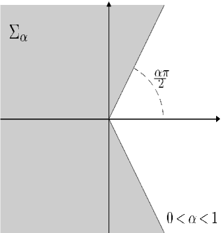
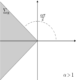
Figure 1: Stability sectors $\Sigma_{\alpha}$ for $0<\alpha<1$ (left) and $\alpha>1$ (right)

When PI rules or FLMMs are applied to (14), the numerical solution $\bigl{\{}y_{n}\bigr{\}}_{n\in\mathbb{N}}$ is evaluated by means of a convolution quadrature

$$y_{n}=g_{n}+z_{\alpha}\sum_{j=0}^{n}\omega_{n-j}y_{j},\quad z_{\alpha}=h^{\alpha}\lambda.$$ (15)

The problem of determining the stability region $S_{\alpha}\subseteq\mathbb{C}$ such that $y_{n}\to 0$ whenever $z_{\alpha}\in S_{\alpha}$ has been discussed in [37, 39] and the main result can be summarized in the following theorem.

Theorem 6.

Let $\alpha>0$. Under the assumption that the sequence $\bigl{\{}g_{n}\bigr{\}}_{n}$ is convergent and that the quadrature weights $\omega_{n}$ satisfy

$$\omega_{n}=\frac{n^{\alpha-1}}{\Gamma(\alpha+1)}+u_{n}\quad\textrm{ with }\quad\sum_{n=1}^{\infty}|u_{n}|<\infty,\quad n\geq 1,$$

the stability region of the convolution quadrature (15) is

$$S_{\alpha}=\mathbb{C}\backslash\left\{\frac{1}{\omega_{\alpha}(\xi)}\,:\>|\xi|\leq 1\right\},\quad\omega_{\alpha}(\xi)=\sum_{n=0}^{\infty}\omega_{n}\xi^{n}.$$

We refer to [23] and [38] to verify that the PI rule and the FLMMs investigated in this paper fulfill the assumptions of Theorem 6.

In the numerical treatment of ODEs $A$–stability means that the whole complex semi–plane is included in the stability region of the method. $A$–stable methods are therefore particularly attractive since they ensure that the numerical solution of stable linear problems converges to $0$ regardless of the size of the step $h$. Because of the result in Theorem 5, for FDEs it is more useful to use the concept of $A(\alpha\frac{\pi}{2})$–stability, which means that the whole sector $\Sigma_{\alpha}$ must be included in the stability region.

While $\omega_{\alpha}(\xi)$ is a priori known for FLMMs, the generating function of PI rules does not possess an analytical representation and, therefore, it can be just numerically approximated.

In Figure 2 we present a comparison of the stability regions (the gray areas) of the methods discussed in the previous sections for various values $0<\alpha<1$ (dotted lines denote the corresponding sectors of stability $\Sigma_{\alpha}$). To identify each method, here and throughout the following section we make use of the acronyms listed in Table 1.

Acronym	Formula	Subsection
PI U	PI rule on uniform grid	3.1
PI G	PI rule on graded grid	3.2
FT	fractional trapezoidal rule	4.1
NG	Newton–Gregory formula	4.2
FBDF	fractional BDF formula	4.3

Table 1: Acronyms used to denote methods

We can distinctly observe that, as $\alpha$ increases from $0$ to $1$, the stability region of each method decreases but always includes $\Sigma_{\alpha}$; we can draw the conclusion that all the methods are $A(\alpha\frac{\pi}{2})$–stable for $0<\alpha<1$.

PI U	FT	NG	FBDF

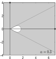
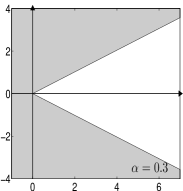
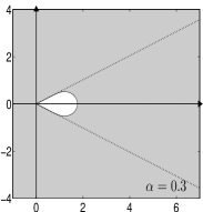
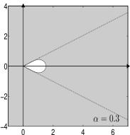
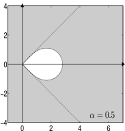
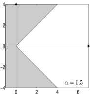
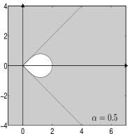
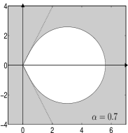
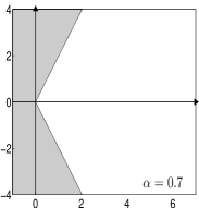
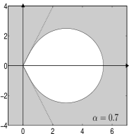
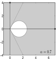
Figure 2: Stability regions (gray areas) for some orders $0<\alpha<1$

Within ODEs, the stability region of the trapezoidal rule is the negative semi–plane $\mathbb{C}^{-}$ and exactly corresponds to the region in which the true solution converges to the steady–state. Among the methods presented in this paper, just FT preserves this feature and indeed its stability regions coincide with $\Sigma_{\alpha}$ for any value of $\alpha$. NG and PI have regions of almost the same size but larger with respect to FT; as in the ODE case, FBDF possesses the largest regions of stability.

Interestingly, the situation is completely different for $1<\alpha<2$ as shown in Figure 3. Whilst the stability regions of FT still coincide with the stability sectors $\Sigma_{\alpha}$ and the stability properties of FBDF still remain the most remarkable ones, we observe that NG and PI completely lose the $A(\alpha\frac{\pi}{2})$–stability. This is an important aspect to be taken into account: despite the implicit nature of these methods, numerical instability can arise when a not sufficiently small step–size is used and, therefore, they seem not suited to solve stiff problems when $1<\alpha<2$.

PI U	FT	NG	FBDF

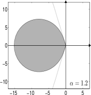
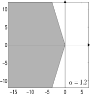
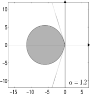
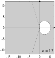
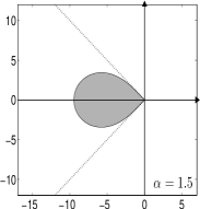
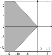
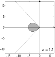
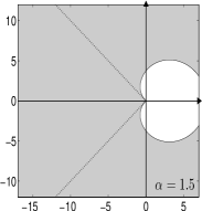
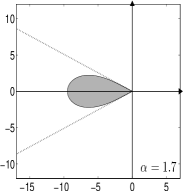
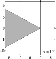
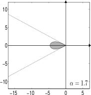
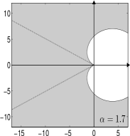
Figure 3: Stability regions (gray areas) for some orders $\alpha>1$

6 Implementation details and Matlab codes

In this section we discuss some implementation issues that are essential for the development of efficient codes.

6.1 Evaluation of the lag term

The evaluation of the (usually long) lag term is one of the most expensive tasks in convolution quadratures like (7) or (10). The integration along a large number $N$ of steps is usually a critical bottleneck and, if not well designed, it can be an impracticable task involving a number of operations proportional to $N^{2}$.

Several authors have discussed this problem (see, for instance, [8]); in [15] a strategy based on parallel algorithms has been described.

In our codes we implement the FFT algorithm described in [28] by which the computational effort downgrades from $N^{2}$ to $N\log(N)^{2}$. We do not further discuss technical details of this algorithm, for which we just refer to the above mentioned paper; we simply observe that, without efficient algorithms of this kind, the numerical solution of FDEs very quickly degenerates in an unworkable task as the number $N$ of grid–points increases.

6.2 Starting weights

Starting weights $w_{n,j}$ are introduced in (10) to cope with the singular behavior of the solution close to the left endpoint of the integration interval. They are evaluated after imposing that (8) is exact for $g(t)=t^{\nu}$ with $\nu\in{\cal A}_{p-1}\cup\bigl{\{}p-1\bigr{\}}$ and $p$ the order of convergence of the FLMM [38].

Because of (3), and since the methods investigated in this paper have order $p=2$, it is immediate to see that weights $w_{n,j}$ must satisfy the relation

$$\sum_{j=0}^{s}w_{n,j}j^{\nu}=-\sum_{j=0}^{n}\omega_{n-j}j^{\nu}+\frac{\Gamma(\nu+1)}{\Gamma(1+\nu+\alpha)}n^{\nu+\alpha},\quad\nu\in{\cal A}_{1}\cup\bigl{\{}1\bigr{\}}$$ (16)

and, hence, they are evaluated by solving, at each step $n$, a system of $s+1$ linear equations, with $s$ the cardinality of ${\cal A}_{1}$.

This problem has been in–depth discussed in [16], where the authors stressed the attention on the mildly ill–conditioned nature of the coefficient matrix $V$ of (16). Nevertheless, for the methods under investigation this is not a serious issue since the size of $V$ is small, being $s=\left\lceil 1/\alpha\right\rceil+1$ (in most cases $s$ will be 3 or 4 and the inversion of $V$ can be done analytically). The only exception is for very small values of $\alpha$ which, however, are extremely uncommon in applications.

6.3 Starting the computation

The initialization of (10) requires the knowledge of the first $s+1$ approximations $y_{0},y_{1},\dots y_{s}$ of the solution. Since just $y_{0}$ is given by the problem, the remaining values must be evaluated in some other way, for instance by using some different methods.

To avoid mixing methods of different nature, we prefer to evaluate all the approximations $y_{1},\dots y_{s}$ at the same time by setting the single implicit system

$$\left(\begin{array}[]{c}y_{1}\\ y_{2}\\ \vdots\\ y_{s}\end{array}\right)=\left(\begin{array}[]{c}T_{m-1}(t_{1})\\ T_{m-1}(t_{2})\\ \vdots\\ T_{m-1}(t_{s})\end{array}\right)+h^{\alpha}\left(\begin{array}[]{c}(\omega_{1}+w_{1,0})f_{0}\\ (\omega_{2}+w_{2,0})f_{0}\\ \vdots\\ (\omega_{s}+w_{s,0})f_{0}\end{array}\right)\\ +h^{\alpha}{\cal B}\left(\begin{array}[]{c}f(t_{1},y_{1})\\ f(t_{2},y_{2})\\ \vdots\\ f(t_{s},y_{s})\end{array}\right),$$

where

$${\cal B}=\left(\begin{array}[]{cccc}\omega_{0}I&&&\\ \omega_{1}I&\omega_{0}I&&\\ \vdots&\vdots&\ddots&\vdots\\ \omega_{s-1}I&\omega_{s-2}I&\dots&\omega_{0}I\end{array}\right)+\left(\begin{array}[]{cccc}w_{1,1}I&w_{1,2}I&\dots&w_{1,s}I\\ w_{2,1}I&w_{2,2}I&\dots&w_{2,s}I\\ \vdots&\vdots&\ddots&\vdots\\ w_{s,1}I&w_{s,2}I&\dots&w_{s,s}I\\ \end{array}\right).$$

This nonlinear system has size $s\cdot q$, where $q$ is the size of the system of FDEs we want to solve. No particular problems arise when the size $q$ of the problem is small; otherwise some memory allocation problems could occur in presence of very small values of $\alpha$, involving a very large number $s$ of initial approximations to compute.

6.4 Solution of the nonlinear systems

All the implicit methods analyzed in Sections 3 and 4 require, at each step, the solution of an algebraic nonlinear system in the form

$$y_{n}=g_{n}+h^{\alpha}\bar{\omega}_{0}f(t_{n},y_{n}),$$

where $g_{n}$ and $\bar{\omega}_{0}$ do not depend on $y_{n}$. To preserve the good stability properties, it is convenient to use Newton iterations

$$y_{n}^{(k+1)}=y_{n}^{(k)}+\Delta^{(k)}_{n},$$

where $\Delta^{(k)}_{n}$ is solution of the linear system

$$A\Delta^{(k)}_{n}=b,\quad A=I-h^{\alpha}\bar{\omega}_{0}J_{f}(y_{n}^{(k)}),\quad b=-y_{n}^{(k)}+g_{n}+h^{\alpha}\bar{\omega}_{0}f(t_{n},y_{n}^{(k)})$$

and, usually, $y_{n}^{(0)}=y_{n-1}$. We refer to [29] for more insights on this issue and for a discussion on the stopping criteria.

We just highlight here that the convergence can depend on $h^{\alpha}$, instead of $h$ as in ODEs. Whilst this is not an issue when $1<\alpha<2$, some unexpected problems could arise whenever $\alpha$ is small. For this reason it is necessary to use a quite small step–size $h$ with low values of $\alpha$.

7 Numerical experiments

By means of numerical experiments we compare the methods discussed in the paper. We perform all the experiments in Matlab, version 7.9.0.529, on a computer equipped with the Intel Dual Core E5400 processor running at 2.70 GHz under the Windows XP operating system; all the Matlab codes have been optimized, to get the best performance, according to the discussion reported in the previous sections.

As a first test problem we consider the linear FDE (14) for $\lambda=-2$. For each method, and for an increasing number $N$ of grid–points, we report the error $E(N)$ at $T=2$, with respect to a reference solution, and we provide an estimation of the order of convergence (EOC) as $\log_{2}(E(N)/E(2N))$.

$$\begin{array}[]{|r|cc|cc|cc|cc|cc|}\hline\cr&\vrule\lx@intercol\hfil\textrm{PI U}\hfil\lx@intercol\vrule\lx@intercol&\vrule\lx@intercol\hfil\textrm{PI G}\hfil\lx@intercol\vrule\lx@intercol&\vrule\lx@intercol\hfil\textrm{FT}\hfil\lx@intercol\vrule\lx@intercol&\vrule\lx@intercol\hfil\textrm{NG}\hfil\lx@intercol\vrule\lx@intercol&\vrule\lx@intercol\hfil\textrm{FBDF}\hfil\lx@intercol\vrule\lx@intercol\\ N&\textrm{Error}&\textrm{EOC}&\textrm{Error}&\textrm{EOC}&\textrm{Error}&\textrm{EOC}&\textrm{Error}&\textrm{EOC}&\textrm{Error}&\textrm{EOC}\\ \hline\cr 32&3.29(-4)&&1.45(-4)&&1.71(-5)&&3.92(-5)&&1.10(-4)&\\ 64&1.15(-4)&1.524&3.65(-5)&1.987&5.65(-6)&1.602&1.20(-5)&1.707&3.16(-5)&1.798\\ 128&4.00(-5)&1.516&9.17(-6)&1.991&1.74(-6)&1.698&3.50(-6)&1.780&8.83(-6)&1.842\\ 256&1.40(-5)&1.511&2.30(-6)&1.993&5.07(-7)&1.779&9.78(-7)&1.838&2.40(-6)&1.880\\ 512&4.94(-6)&1.508&5.78(-7)&1.994&1.41(-7)&1.844&2.65(-7)&1.883&6.37(-7)&1.912\\ 1024&1.74(-6)&1.505&1.45(-7)&1.992&3.77(-8)&1.903&6.98(-8)&1.924&1.66(-7)&1.939\\ 2048&6.14(-7)&1.503&3.67(-8)&1.987&9.49(-9)&1.991&1.77(-8)&1.978&4.25(-8)&1.969\\ \hline\cr\end{array}$$

Table 2: Errors and EOC at $T=2.0$ for the linear FDE (14) with $\alpha=0.5$ and $\lambda=-2.0$

The numerical results in Table 2 for $\alpha=0.5$ clearly confirm theoretical findings on the order of convergence. As expected from Theorem 1, the PI rule on uniform grids fails to obtain order 2 and converges with order $1+\alpha$; on the other hand, the PI rule on graded grids converges with full order $2$.

As in the ODE case, FT produces the smallest error. Although also NG and PI are generalizations of the trapezoidal rule, it seems that only FT inherits this feature; by taking into account, from the analysis of Section 5, that FT preserves the other peculiar character of the trapezoidal rule of having the region of stability exactly equal to the region in which the solution converges towards the steady state, it is tempting to conclude that FT is the most natural generalization of the trapezoidal rule.

Unfortunately, the situation is more complicate since when $1<\alpha<2$ it is NG that provides the lowest error, as shown in Table 3 for $\alpha=1.5$.

$$\begin{array}[]{|r|cc|cc|cc|cc|cc|}\hline\cr&\vrule\lx@intercol\hfil\textrm{PI U}\hfil\lx@intercol\vrule\lx@intercol&\vrule\lx@intercol\hfil\textrm{PI G}\hfil\lx@intercol\vrule\lx@intercol&\vrule\lx@intercol\hfil\textrm{FT}\hfil\lx@intercol\vrule\lx@intercol&\vrule\lx@intercol\hfil\textrm{NG}\hfil\lx@intercol\vrule\lx@intercol&\vrule\lx@intercol\hfil\textrm{FBDF}\hfil\lx@intercol\vrule\lx@intercol\\ N&\textrm{Error}&\textrm{EOC}&\textrm{Error}&\textrm{EOC}&\textrm{Error}&\textrm{EOC}&\textrm{Error}&\textrm{EOC}&\textrm{Error}&\textrm{EOC}\\ \hline\cr 64&3.71(-5)&&6.16(-5)&&5.50(-5)&&1.55(-5)&&1.95(-4)&\\ 128&9.31(-6)&1.993&1.54(-5)&2.000&1.39(-5)&1.988&3.73(-6)&2.053&5.22(-5)&1.902\\ 256&2.33(-6)&1.997&3.85(-6)&2.001&3.48(-6)&1.993&9.10(-7)&2.035&1.35(-5)&1.951\\ 512&5.82(-7)&2.003&9.59(-7)&2.004&8.71(-7)&1.999&2.22(-7)&2.035&3.43(-6)&1.975\\ 1024&1.43(-7)&2.024&2.37(-7)&2.016&2.16(-7)&2.013&5.25(-8)&2.081&8.65(-7)&1.989\\ 2048&3.32(-8)&2.106&5.67(-8)&2.064&5.15(-8)&2.068&1.05(-8)&2.325&2.15(-7)&2.008\\ \hline\cr\end{array}$$

Table 3: Errors and EOC at $T=2.0$ for the linear FDE (14) with $\alpha=1.5$ and $\lambda=-2.0$

This phenomenon can be more clearly observed in Figure 4, where we show the errors as a function of $\alpha$ (we used the same values for $\lambda$ and $T$ from the previous experiment and a fixed number $N=1024$ of grid points).

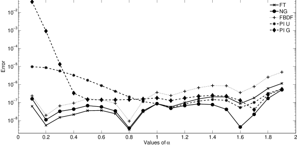
Figure 4: Errors at $T=2.0$ for the linear FDE (14) with $\lambda=-2.0$ and $N=1024$.

We must highlight that this is a not completely unexpected result. Stability and accuracy are indeed conflicting requirements in most of numerical methods; thus, FT shows the smallest regions of stability but the lowest error when $0<\alpha<1$, exactly as it happens with NG for $1<\alpha<2$. What we observe is a kind of roles swap between FT and NG when $\alpha$ moves from the left to the right of 1.

The very bad performance of PI on graded grids for low values of $\alpha$ is due to the fact that the grids generated by the graded exponent $r=2\alpha$ are very coarse close to right endpoint of the integration interval. Furthermore, graded grids do not add any improvement for $\alpha>1$, since the maximum expected order $2$ is already achieved by using uniform grids. We can draw the conclusion that the utility of graded grids is confined only to $\frac{1}{2}<\alpha<1$.

It is also interesting to analyze the computational effort in relation to the accuracy. To this purpose, the plots in Figure 5, which are related to the experiments presented in Tables 2 and 3, show that FT, NG and FBDF behave in a more efficient way with respect to PI when $0<\alpha<1$; indeed, PI U pays for the reduction in the accuracy whilst PI G pays for the absence of a convolution structure which precludes the application of FFT algorithms. The minor efficiency of FBDF with respect to FT and NG is due to the major complexity in the evaluation of weights. It is worthwhile to note that the preeminence of FLMMs with respect to PI rules holds despite the need of solving linear systems for evaluating the starting weights. For $1<\alpha<2$ the absence of order reduction increases the efficiency of PI on uniform nodes but however it is below that of NG which instead has lower errors.

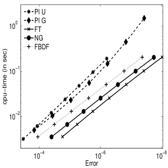
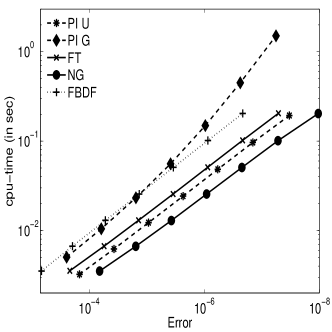
Figure 5: Errors versus time of execution for $\alpha=0.5$ (left) and $\alpha=1.5$ (right)

To observe the behavior of the methods under investigation for nonlinear problems, we consider the fractional reaction diffusion system of Brusselator type

$$\left\{\begin{array}[]{l}{}^{C}D^{\alpha}_{t_{0}}x_{1}(t)=a-(\mu+1)x_{1}(t)+x_{1}(t)^{2}x_{2}(t)\\ {}^{C}D^{\alpha}_{t_{0}}x_{2}(t)=\mu x_{1}(t)-x_{1}(t)^{2}x_{2}(t)\end{array}\right..$$ (17)

It has been shown [20] that there exists a marginal value $\bar{\alpha}$, depending on $a$ and $\mu$, such that system (17) approaches a stable limit cycle, as shown in Figure 6 for $\alpha=0.8$ and $(a,\mu)=(1,4)$.

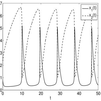
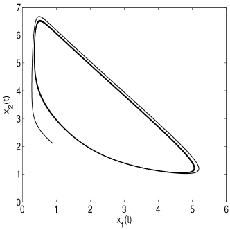
Figure 6: Solution of the fractional Brusselator system (17) for $\alpha=0.8$ and $(a,\mu)=(1,4)$ in the $(t,x)$-plane (left) and in the phase plane (right)

$$\begin{array}[]{|r|cc|cc|cc|cc|cc|}\hline\cr&\vrule\lx@intercol\hfil\textrm{PI U}\hfil\lx@intercol\vrule\lx@intercol&\vrule\lx@intercol\hfil\textrm{PI G}\hfil\lx@intercol\vrule\lx@intercol&\vrule\lx@intercol\hfil\textrm{FT}\hfil\lx@intercol\vrule\lx@intercol&\vrule\lx@intercol\hfil\textrm{NG}\hfil\lx@intercol\vrule\lx@intercol&\vrule\lx@intercol\hfil\textrm{FBDF}\hfil\lx@intercol\vrule\lx@intercol\\ N&\textrm{Error}&\textrm{EOC}&\textrm{Error}&\textrm{EOC}&\textrm{Error}&\textrm{EOC}&\textrm{Error}&\textrm{EOC}&\textrm{Error}&\textrm{EOC}\\ \hline\cr 400&3.66(-1)&&7.33(-1)&&2.88(-1)&&3.67(-1)&&5.23(-1)&\\ 800&6.04(-2)&2.601&2.55(-1)&1.523&5.12(-2)&2.490&6.32(-2)&2.537&1.50(-1)&1.800\\ 1600&1.55(-2)&1.965&5.66(-2)&2.173&1.28(-2)&2.005&1.63(-2)&1.956&4.31(-2)&1.798\\ 3200&4.00(-3)&1.953&1.35(-2)&2.064&3.27(-3)&1.964&4.21(-3)&1.951&1.19(-2)&1.864\\ 6400&1.01(-3)&1.982&3.37(-3)&2.006&8.27(-4)&1.982&1.07(-3)&1.982&3.12(-3)&1.926\\ 12800&2.41(-4)&2.071&8.33(-4)&2.015&1.94(-4)&2.095&2.55(-4)&2.065&7.92(-4)&1.977\\ \hline\cr\end{array}$$

Table 4: Errors and EOC at $T=50.0$ for the Brusselator system (17) with $\alpha=0.8$

From Table 4 the good results provided by PI U stand out. This is an indirect evidence that the findings of Theorem 1 can be quite pessimistic in some cases; indeed, the drop in the convergence order depends on the expansion of the vector field which in some cases could not involve real powers of low degree. However, also in this case FT presents the smallest error.

The relationship between errors and execution times in Figure 7 shows however that the efficiency of PI U, also in this favourable case, can be at least comparable but not higher with respect to FT and NG; it is hence quite difficult to justify the major attention that PI rules usually attract in the literature on the numerical solution of FDEs.

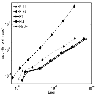
Figure 7: Errors versus time of execution for the Brusselator system (17) with $\alpha=0.8$

8 Concluding remarks

In this paper we have discussed some implicit second order methods for FDEs and investigated some of the main aspects related to their efficient implementation.

We have observed that stability properties change according to the value of the fractional order $\alpha$ and whenever $1<\alpha<2$ the NG and PI are no longer $A(\alpha\frac{\pi}{2})$–stable. As in the ODE case, the method obtained starting from BDF shows the largest stability regions.

Whilst FT provides the smallest error for $0<\alpha<1$, the performance of NG stands out for $1<\alpha<2$ . PI rules with graded grids appear effective just for $\alpha$ between $\frac{1}{2}$ and $1$; anyway, it seems that in general the overall efficiency of FLMMs is superior to PI, despite the major interest that PI rules usually attract.

References

- [1] Brunner, H. The numerical solution of weakly singular Volterra integral equations by collocation on graded meshes. Math. Comp. 45, 172 (1985), 417–437.
- [2] Brunner, H. Collocation methods for Volterra integral and related functional differential equations. Cambridge University Press, Cambridge, 2004.
- [3] Bueno-Orovio, A., Kay, D., Grau, V., Rodriguez, B., and Burrage, K. Fractional diffusion models of cardiac electrical propagation : role of structural heterogeneity in dispersion of repolarization. Tech. Rep. OCCAM 13/35, Oxford Centre for Collaborative Applied Mathematics, Oxford (UK), 2013.
- [4] Burrage, K., Hale, N., and Kay, D. An efficient implicit FEM scheme for fractional-in-space reaction-diffusion equations. SIAM J. Sci. Comput. 34, 4 (2012), A2145–A2172.
- [5] Cafagna, D., and Grassi, G. Observer-based projective synchronization of fractional systems via a scalar signal: Application to hyperchaotic Rössler systems. Nonlinear Dynamics 68, 1-2 (2012), 117–128.
- [6] Cameron, R. F., and McKee, S. The analysis of product integration methods for Abel’s equation using discrete fractional differentiation. IMA J. Numer. Anal. 5, 1 (1985), 339–353.
- [7] Caponetto, R., Maione, G., Pisano, A., Rapaić, M. M. R., and Usai, E. Analysis and shaping of the self-sustained oscillations in relay controlled fractional-order systems. Fractional Calculus and Applied Analysis 16, 1 (2013), 93–108.
- [8] Conte, D., and Prete, I. D. Fast collocation methods for Volterra integral equations of convolution type. J. Comput. Appl. Math. 196, 2 (2006), 652–663.
- [9] de Hoog, F., and Weiss, R. High order methods for a class of Volterra integral equations with weakly singular kernels. SIAM J. Numer. Anal. 11 (1974), 1166–1180.
- [10] Dieci, L., and Lopez, L. Sliding motion in Filippov differential systems: theoretical results and a computational approach. SIAM J. Numer. Anal. 47, 3 (2009), 2023–2051.
- [11] Dieci, L., and Lopez, L. Sliding motion on discontinuity surfaces of high co-dimension. A construction for selecting a Filippov vector field. Numer. Math. 117, 4 (2011), 779–811.
- [12] Dieci, L., and Lopez, L. A survey of numerical methods for IVPs of ODEs with discontinuous right-hand side. J. Comput. Appl. Math. 236, 16 (2012), 3967–3991.
- [13] Diethelm, K. An investigation of some nonclassical methods for the numerical approximation of Caputo-type fractional derivatives. Numer. Algorithms 47, 4 (2008), 361–390.
- [14] Diethelm, K. The analysis of fractional differential equations, vol. 2004 of Lecture Notes in Mathematics. Springer-Verlag, Berlin, 2010.
- [15] Diethelm, K. An efficient parallel algorithm for the numerical solution of fractional differential equations. Fract. Calc. Appl. Anal. 14, 3 (2011), 475–490.
- [16] Diethelm, K., Ford, J. M., Ford, N. J., and Weilbeer, M. Pitfalls in fast numerical solvers for fractional differential equations. J. Comput. Appl. Math. 186, 2 (2006), 482–503.
- [17] Diethelm, K., Ford, N. J., Freed, A. D., and Luchko, Y. Algorithms for the fractional calculus: a selection of numerical methods. Comput. Methods Appl. Mech. Engrg. 194, 6-8 (2005), 743–773.
- [18] Diethelm, K., and Freed, A. D. The FracPECE subroutine for the numerical solution of differential equations of fractional order. In Forschung und wissenschaftliches Rechnen 1998, S.Heinzel and T.Plesser, Eds. 1999, pp. 57–71.
- [19] Dixon, J. On the order of the error in discretization methods for weakly singular second kind Volterra integral equations with nonsmooth solutions. BIT 25, 4 (1985), 624–634.
- [20] Gafiychuk, V. V., and Datsko, B. Stability analysis and limit cycle in fractional system with Brusselator nonlinearities. Physics Letters A 372, 29 (2008), 4902 – 4904.
- [21] Galeone, L., and Garrappa, R. Fractional Adams-Moulton methods. Math. Comput. Simulation 79, 4 (2008), 1358–1367.
- [22] Garra, R. Fractional-calculus model for temperature and pressure waves in fluid-saturated porous rocks. Phys. Rev. E 84 (Sep 2011), 036605.
- [23] Garrappa, R. On linear stability of predictor–corrector algorithms for fractional differential equations. Int. J. Comput. Math. 87, 10 (2010), 2281–2290.
- [24] Garrappa, R. On some generalizations of the implicit Euler method for discontinuous fractional differential equations. Math. Comput. Simulat. (2012).
- [25] Garrappa, R., and Popolizio, M. On accurate product integration rules for linear fractional differential equations. J. Comput. Appl. Math. 235, 5 (2011), 1085–1097.
- [26] Garrappa, R., and Popolizio, M. Evaluation of generalized Mittag–Leffler functions on the real line. Adv. Comput. Math. 39, 1 (2013), 205–225.
- [27] Gorenflo, R. Fractional calculus: some numerical methods. In Fractals and Fractional Calculus in Continuum Mechanics, A. Carpinteri and F. Mainardi, Eds., vol. 278 of CISM Courses and Lectures. Springer Verlag, Wien and New York, 1997, pp. 277–290.
- [28] Hairer, E., Lubich, C., and Schlichte, M. Fast numerical solution of nonlinear Volterra convolution equations. SIAM J. Sci. Statist. Comput. 6, 3 (1985), 532–541.
- [29] Hairer, E., and Wanner, G. Solving ordinary differential equations. II, second ed. Springer-Verlag, Berlin, 1996.
- [30] Henrici, P. Applied and computational complex analysis, vol. 1. John Wiley & Sons, New York, 1974.
- [31] Henrici, P. Fast Fourier methods in computational complex analysis. SIAM Rev. 21, 4 (1979), 481–527.
- [32] Kadem, A., Luchko, Y., and Baleanu, D. Spectral method for solution of the fractional transport equation. Rep. Math. Phys. 66, 1 (2010), 103–115.
- [33] Kilbas, A. A., Srivastava, H. M., and Trujillo, J. J. Theory and applications of fractional differential equations, vol. 204 of North-Holland Mathematics Studies. Elsevier Science B.V., Amsterdam, 2006.
- [34] Lambert, J. D. Numerical methods for ordinary differential systems. John Wiley & Sons Ltd., Chichester, 1991.
- [35] Li, C., and Zeng, F. The finite difference methods for fractional ordinary differential equations. Numer. Funct. Anal. Optim. 34, 2 (2013), 149–179.
- [36] Lubich, C. Runge-Kutta theory for Volterra and Abel integral equations of the second kind. Math. Comp. 41, 163 (1983), 87–102.
- [37] Lubich, C. Fractional linear multistep methods for Abel–Volterra integral equations of the second kind. Math. Comp. 45, 172 (1985), 463–469.
- [38] Lubich, C. Discretized fractional calculus. SIAM J. Math. Anal. 17, 3 (1986), 704–719.
- [39] Lubich, C. A stability analysis of convolution quadratures for Abel-Volterra integral equations. IMA J. Numer. Anal. 6, 1 (1986), 87–101.
- [40] Machado, J. T., Kiryakova, V., and Mainardi, F. Recent history of fractional calculus. Commun. Nonlinear Sci. Numer. Simul. 16, 3 (2011), 1140–1153.
- [41] Magin, R. L. Fractional calculus models of complex dynamics in biological tissues. Computers & Mathematics with Applications 59, 5 (2010), 1586 – 1593.
- [42] Mainardi, F. Fractional calculus and waves in linear viscoelasticity. Imperial College Press, London, 2010.
- [43] Matignon, D. Stability properties for generalized fractional differential systems. In Systèmes différentiels fractionnaires (Paris, 1998), vol. 5 of ESAIM Proc. Soc. Math. Appl. Indust., Paris, 1998, pp. 145–158.
- [44] Meerschaert, M. M., and Tadjeran, C. Finite difference approximations for fractional advection-dispersion flow equations. J. Comput. Appl. Math. 172, 1 (2004), 65–77.
- [45] Meerschaert, M. M., and Tadjeran, C. Finite difference approximations for two-sided space-fractional partial differential equations. Appl. Numer. Math. 56, 1 (2006), 80–90.
- [46] Moret, I. A note on Krylov methods for fractional evolution problems. Numer. Func. Anal. Opt. 34, 5 (2013), 539–556.
- [47] Moret, I., and Novati, P. On the convergence of Krylov subspace methods for matrix Mittag-Leffler functions. SIAM J. Numer. Anal. 49, 5 (2011), 2144–2164.
- [48] Moret, I., and Popolizio, M. The restarted shift-and-invert Krylov method for matrix functions. Numerical Linear Algebra with Applications (2012).
- [49] Podlubny, I. Fractional differential equations, vol. 198 of Mathematics in Science and Engineering. Academic Press Inc., San Diego, CA, 1999.
- [50] Tenreiro Machado, J., Stefanescu, P., Tintareanu, O., and Baleanu, D. Fractional calculus analysis of the cosmic microwave background. Romanian Reports in Physics 65, 1 (2013), 316–323.
- [51] Wolkenfelt, P. H. M. Linear multistep methods and the construction of quadrature formulae for volterra integral and integro-differential equations. Tech. Rep. NW 76/79, Mathematisch Centrum,, Amsterdam (Netherlands), 1979.
- [52] Young, A. Approximate product-integration. Proc. Roy. Soc. London Ser. A. 224 (1954), 552–561.
- [53] Yuste, S. B., and Acedo, L. An explicit finite difference method and a new von Neumann-type stability analysis for fractional diffusion equations. SIAM J. Numer. Anal. 42, 5 (2005), 1862–1874.
- [54] Yuste, S. B., and Quintana-Murillo, J. A finite difference method with non-uniform timesteps for fractional diffusion equations. Comput. Phys. Commun. 183, 12 (2012), 2594–2600.