Quantum radiation in dielectric media with dispersion and dissipation

Abstract

By a generalization of the Hopfield model, we construct a microscopic Lagrangian describing a dielectric medium with dispersion and dissipation. This facilitates a well-defined and unambiguous ab initio treatment of quantum electrodynamics in such media, even in time-dependent backgrounds. As an example, we calculate the number of photons created by switching on and off dissipation in dependence on the temporal switching function. This effect may be stronger than quantum radiation produced by variations of the refractive index $\Delta n(t)$ since the latter are typically very small and yield photon numbers of order $(\Delta n)^{2}$. As another difference, we find that the partner particles of the created medium photons are not other medium photons but excitations of the environment field causing the dissipation (which is switched on and off).

I Introduction

One of the most striking consequences of quantum field theory is the non-trivial nature of the vacuum or ground state. Even in this lowest-energy state, fields do not vanish identically, but are permanently fluctuating. These quantum vacuum fluctuations cause many well-known effects such as spontaneous emission [1], the Casimir effect [2], or the Lamb shift [3, 4]. Another fascinating consequence is the phenomenon of quantum radiation, where these fluctuations are converted into real particles by suitable external conditions, which would have no effect on the classical vacuum (with all fields vanishing identically). Examples include Hawking radiation [5, 6], the dynamical Casimir effect [7], and cosmological particle creation [8, 9]; but also time (or even space-time) dependent variations of the refractive index in dielectric media (or waveguides), where the latter can display interesting analogies [10, 11, 12] to the former ones, see also Refs. [13, 14, 15, 16, 17, 18, 19, 20, 21, 22, 23, 24, 25, 26, 27], [28, 29, 30, 31] and [32, 33, 34], respectively.

In a notably simplified approach, aspects of quantum radiation can be studied by neglecting medium properties such as dispersion and dissipation. Going beyond this simple picture, there has been considerable work regarding the effects of dispersion, see, e.g., [21, 35, 22, 23, 24, 25, 27]. However, in the vast majority of publications, quantum radiation has been considered in absence of dissipation, with a few exceptions including [36, 37, 38]. One of the main reasons lies in the intrinsic difficulty of treating dissipation correctly, especially regarding quantum fluctuations under non-trivial external conditions.

There are basically two main approaches for adding dissipation to the well-established theory of non-dissipative dielectrics discussed in, e.g., [39, 40, 41]. In a top-down approach, one starts with the phenomenological properties of a given medium such as the complex dielectric permittivity $\varepsilon(\omega)$ and then constructs the corresponding quantum field operators by demanding consistency conditions, see, e.g., [42, 43, 44, 45]. The alternative bottom-up approach, on the other hand, is based on microscopic models, which allow for deriving the associated medium properties such as $\varepsilon(\omega)$. For simple cases, such as stationary and homogeneous media, it is possible to show the equivalence of these two approaches via the Huttner-Barnett formalism [46, 47, 48] based on an exact Fano diagonalization [49, 50, 51]. However, extending this formalism to more general cases such as temporally and possibly even spatio-temporally varying media is quite involved. Thus, even though the phenomenological approach has the obvious advantage to account for media with very general $\varepsilon(\omega)$, it has the drawback of potential ambiguities, especially in time-dependent scenarios.

A related issue is the explicit calculation of observables (e.g., the number of created photons) which typically requires certain approximations. In order to describe dissipative media, several microscopic approaches employ a Markov-type approximation (e.g., in Weisskopf-Wigner theory) which neglects the memory of the environment, see also [52]. Especially in time-dependent scenarios, the justification and applicability of such an approximation must be scrutinized in order to avoid inconsistencies.

In the following, we propose and study an explicit microscopic model (bottom-up approach) for a 1+1 dimensional dielectric medium including dispersion and dissipation, which does not require any Markov-type approximations and has well defined in and out states. The goal is an ab inito treatment of quantum radiation without ambiguities and additional assumptions. Using this approach, we study quantum radiation emerging from time-dependent variations (switching on and off) in the coupling between a medium and its environment, see also [53, 54, 55, 56].

II The Model

We consider the following Lagrangian

$$L=L_{A}+L_{\Psi}+L_{A\Psi}+L_{\Phi}+L_{\Psi\Phi}\,,$$ (1)

where $L_{A}$ describes the electromagnetic vector potential $A(t,x)$ in 1+1 dimensions ($\hbar=c=1$)

$$L_{A}=\frac{1}{2}\int dx\,\left\{\left[\partial_{t}A(t,x)\right]^{2}-\left[\partial_{x}A(t,x)\right]^{2}\right\}\,.$$ (2)

As usual in the Hopfield model, the polarization of the medium is included by adding harmonic oscillators $\Psi(t,x)$ with resonance frequency $\Omega>0$ to all points $x$ of the dielectric

$$L_{\Psi}=\frac{1}{2}\int dx\,\left\{\left[\partial_{t}\Psi(t,x)\right]^{2}-\Omega^{2}\Psi^{2}(t,x)\right\}\,,$$ (3)

and coupling them to the electric field $E=-\partial_{t}A$ via

$$L_{A\Psi}=-g\int dx\,\Psi(t,x)\partial_{t}A(t,x)\,,$$ (4)

with the coupling strength $g$.

The above terms $L_{A}+L_{\Psi}+L_{A\Psi}$ represent the usual Hopfield model [39, 40, 41, 24]. In order to include dissipation, we introduce an additional field $\Phi(t,x,y)$ which can exchange energy with the medium and propagates in a perpendicular ($y$) direction

$$L_{\Phi}=\frac{1}{2}\int dx\,dy\,\left\{\left[\partial_{t}\Phi(t,x,y)\right]^{2}-\left[\partial_{y}\Phi(t,x,y)\right]^{2}\right\}\,.$$ (5)

This field is coupled to the medium $\Psi(t,x)$ in the same way as the electromagnetic field $A(t,x)$, but with a coupling strength $G$

$$L_{\Psi\Phi}=-G\int dx\,\Psi(t,x)\partial_{t}\Phi(t,x,y=0)\,,$$ (6)

where we assume the medium to be located along the $y=0$ line.

In principle, this model holds for media with general time-dependent parameters $\Omega$, $g$ and $G$, and can even be generalized to fully space-time dependent settings.

III Equations of Motion

In order to show that the above model (1) does indeed feature the dynamics expected for a dissipative medium, let us study the associated Euler-Lagrange equations. For the electromagnetic field $A(t,x)$, we obtain the same form as in the usual Hopfield model

$$\left[\partial_{t}^{2}-\partial_{x}^{2}\right]A(t,x)=\partial_{t}\left[g\Psi(t,x)\right]\,,$$ (7)

but the medium field $\Psi(t,x)$ acquires an additional term

$$\left[\partial_{t}^{2}+\Omega^{2}\right]\Psi(t,x)=-g\partial_{t}A(t,x)-G\partial_{t}\Phi(t,x,0)\,.$$ (8)

Finally, the environment field $\Phi(t,x,y)$ evolves according to

$$\left[\partial_{t}^{2}-\partial_{y}^{2}\right]\Phi(t,x,y)=\partial_{t}\left[G\Psi(t,x)\right]\delta(y)\,,$$ (9)

where we have written all equations is such a way that they equally hold for time-dependent $\Omega(t)$, $g(t)$ and $G(t)$.

III.1 Dispersion relation

Considering constant parameters ($\Omega$, $g$ and $G$) for the moment, we may solve Eq. (9) via the retarded Green’s function and arrive at

$$\Phi(t,x,y)=\Phi_{0}(t,x,y)+\frac{G}{2}\Psi(t-|y|,x)\,,$$ (10)

where $\Phi_{0}(t,x,y)$ denotes the homogeneous solution of Eq. (9), i.e., of $\left[\partial_{t}^{2}-\partial_{y}^{2}\right]\Phi_{0}(t,x,y)=0$. Since we have used the retarded Green’s function (with the retarded time argument $t-|y|$), this solution $\Phi_{0}(t,x,y)$ describes the environment field originating from $\mathcal{I}^{-}$ (i.e., $t\to-\infty$ and $y\to\pm\infty$) before interacting with the medium at $y=0$.

Inserting this solution back into Eq. (8), we get a driven and damped oscillator at each position $x$

$$\left[\partial_{t}^{2}+\frac{G^{2}}{2}\,\partial_{t}+\Omega^{2}\right]\Psi(t,x) = -G\partial_{t}\Phi_{0}(t,x,y=0)$$ (11)

$$-g\partial_{t}A(t,x)\,,$$

where we can read off the damping factor $\Gamma=G^{2}/4$ of the medium. By finally combining Eqs. (7) and (11), we find (for constant $\Omega$, $g$ and $G$)

$$\left[\left(\partial_{t}^{2}+\frac{G^{2}}{2}\,\partial_{t}+\Omega^{2}\right)\left(\partial_{t}^{2}-\partial_{x}^{2}\right)+g^{2}\partial_{t}^{2}\right]A(t,x)=$$

$$-gG\partial_{t}^{2}\Phi_{0}(t,x,y=0)\,.\quad$$ (12)

The environment field on the right-hand side constitutes the classical counterpart of the quantum noise term required by the fluctuation-dissipation theorem while the differential operator on the left-hand side yields the dispersion relation

$$k^{2}=\omega^{2}\left(1+\frac{g^{2}}{\Omega^{2}-i\omega G^{2}/2-\omega^{2}}\right)=\omega^{2}\varepsilon(\omega)\,,$$ (13)

which turns into a standard textbook expression (see, e.g., Sec. 11.3 of Ref. [57]) for dissipative dielectric media after some minor rescaling of system parameters.

From the corresponding dielectric permittivity $\varepsilon(\omega)$ illustrated in Fig. 1, we obtain the effective refractive index $n=\sqrt{1+g^{2}/\Omega^{2}}$ for small photon frequencies $\omega$. The imaginary part

$$\Im[\varepsilon(\omega)]=2\Gamma\,\frac{n^{2}-1}{\Omega^{2}}\,\omega+{\cal O}(\omega^{2})$$ (14)

is closely linked to the damping exponent of solutions

$$A(t,x)\propto\exp{\left\{i\omega\sqrt{\varepsilon(\omega)}x-i\omega t\right\}}$$ (15)

which oscillate at frequencies $\omega>0$ where

$$\Im\left\{\sqrt{\varepsilon(\omega)}\right\}=\Gamma\,\frac{n^{2}-1}{n\Omega^{2}}\,\omega+\mathcal{O}\left(w^{2}\right)\,.$$ (16)

Note that this quantity is related to but not identical with the intrinsic damping $\Gamma=G^{2}/4$ of the oscillators $\Psi(t,x)$.

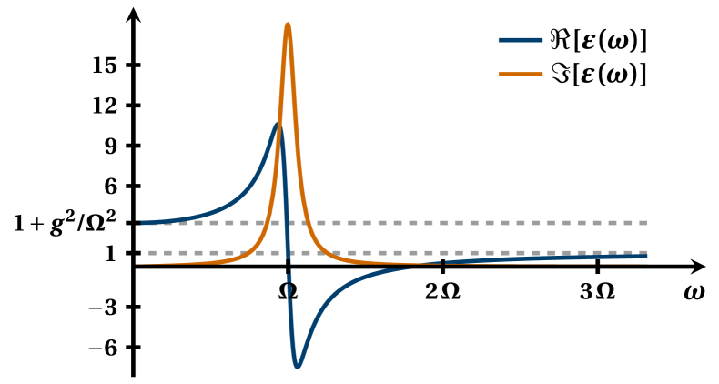
Figure 1: Real and imaginary parts of the dielectric permittivity $\varepsilon(\omega)$ for exemplary parameters $g=3\Omega/2$ and $G=\sqrt{\Omega}/2$, i.e., in the underdamped regime of $G^{2}<4\Omega$.

IV Quantization

As an advantage of our microscopic model (1), we may now derive the corresponding quantum field operators $\hat{A}$, $\hat{\Psi}$, and $\hat{\Phi}$ in an unambiguous manner which consistently takes the quantum fluctuations of all fields into account. The origin of those fluctuations depends on the time-dependence of the coupling parameters $g(t)$ and $G(t)$. If both adopt finite values for a sufficiently long time, extending far into the past, all quantum fluctuations can ultimately be traced back to vacuum fluctuations of the environment field $\hat{\Phi}_{0}$. However, if that field is initially decoupled from the remaining ones $\hat{A}$ and $\hat{\Psi}$ (the case we shall consider later), the $\hat{A}$ and $\hat{\Psi}$ fields will bring in their own initial quantum fluctuations. Then, if $G(t)$ is switched on, all these fluctuations become mixed – which gives rise to particle creation.

IV.1 Environment Field $\Phi_{0}$

Let us first consider the impact of the environment field. In the general case of time-dependent parameters $\Omega(t)$, $g(t)$ and $G(t)$, the equations of motion (7), (8) and (9) can be decoupled analogous to the scenario of a static medium. For example, the solution of Eq. (9) for time-dependent $G(t)$ has the same form as in Eq. (10) but with the modified argument $G(t-|y|)$. Inserting this solution back into Eqs. (7) and (8), we may decouple these two second-order equations into one fourth-order equation for the medium field

$$\left\{\left[\partial_{t}^{2}-\partial_{x}^{2}\right]\frac{1}{g}\left[\partial_{t}^{2}+\frac{1}{2}G\partial_{t}G+\Omega^{2}\right]+\partial_{t}^{2}g\right\}\hat{\Psi}(t,x)=$$

$$-\left[\partial_{t}^{2}-\partial_{x}^{2}\right]\frac{G}{g}\partial_{t}\hat{\Phi}_{0}(t,x,y=0)\,,\quad$$ (17)

where we have omitted the arguments $t$ of all system parameters $\Omega$, $g$ and $G$ to enhance readability. After solving Eq. (IV.1), the corresponding electromagnetic field $\hat{A}(t,x)$ can finally be obtained via integration of Eq. (8).

If the initial $G(t\to-\infty)$ is non-vanishing, the homogeneous solutions of the above equation decay with time and thus only the inhomogeneous solution stemming from the source term on the right-hand side survives. In other words, the initial quantum fluctuations of the fields $\hat{A}$ and $\hat{\Psi}$ are transferred (i.e., lost) to the environment and all the remaining quantum fluctuations stem from the primordial fluctuations of $\hat{\Phi}_{0}$.

As explained above, this homogeneous solution $\hat{\Phi}_{0}(t,x,y)$ constitutes a free scalar field in two spatial dimensions, albeit with a non-isotropic dispersion relation $\omega=|k_{y}|$ as it propagates in $y$ direction only. Thus, it can be quantized in the usual manner

$$\hat{\Phi}_{0}(t,\mbox{\boldmath$r$})=\int\frac{d^{2}k}{2\pi}\;\frac{\hat{b}_{\mbox{\boldmath$\scriptstyle k$}}\,\exp\{i\mbox{\boldmath$k$}\cdot\mbox{\boldmath$r$}-i|k_{y}|t\}}{\sqrt{2|k_{y}|}}+{\rm h.c.}$$ (18)

with standard bosonic creation and annihilation operators $\hat{b}_{\mbox{\boldmath$\scriptstyle k$}}^{\dagger}$ and $\hat{b}_{\mbox{\boldmath$\scriptstyle k$}}$ satisfying $[\hat{b}_{\mbox{\boldmath$\scriptstyle k^{\phantom{\prime}}$}}^{\phantom{\dagger}},\hat{b}_{{\mbox{\boldmath$\scriptstyle k^{\prime}$}}}^{\dagger}]=\delta^{2}(\mbox{\boldmath$k$}-\mbox{\boldmath$k^{\prime}$})$. They correspond to the initial vacuum state $\ket{0}_{\rm in}$ of the environment field (incoming from $\mathcal{I}^{-}$) with $\hat{b}_{\mbox{\boldmath$\scriptstyle k$}}\ket{0}_{\rm in}=0$. In the following, we will use the notation $k_{y}\to\kappa$ and $k_{x}\to k$ for reasons of convenience.

IV.2 Decoupled Case

As pointed out at the beginning of this section, the situation is different for an initially non-dissipative (albeit still dispersive) medium. In this case, the coupled $A$-$\Psi$ system is decoupled from the $\Phi$ field and thus both start to evolve from their independent vacuum states. For $G=0$ and non-vanishing, constant $\Omega$ and $g$, we have the usual Hopfield Hamiltonian $\hat{H}_{\rm H}$ which can be diagonalized [40] via

$$:\!\hat{H}_{\rm H}\!:\;=\sum_{\pm}\int dk\,\omega_{\pm}(k)\hat{a}^{\dagger}_{\pm}(k)\hat{a}_{\pm}(k)\,,$$ (19)

with $\hat{a}^{\dagger}_{\pm}(k)$ and $\hat{a}_{\pm}(k)$ denoting the creation and annihilation operators of the two bands

$$\omega_{\pm}(k)=\sqrt{\frac{(k^{2}+\Omega^{2}+g^{2})\pm\rho(k)}{2}}\,,$$ (20)

where we have used the abbreviations

$$\rho(k)=\sqrt{4k^{2}g^{2}+\sigma^{2}(k)}$$ (21)

and

$$\sigma(k)=k^{2}-g^{2}-\Omega^{2}\,.$$ (22)

As illustrated in Fig. 2, the lower band $\omega_{-}(k)$ behaves as $|k|/n$ for small $k$, while the upper band $\omega_{+}(k)$ tends to a constant value $\sqrt{\Omega^{2}+g^{2}}=n\Omega$. For large $k$, on the other hand, the lower band $\omega_{-}(k)$ approaches the medium resonance frequency $\Omega$ while the upper band reaches the vacuum light cone $|k|$. In contrast to the lower band accounting for massless photons at small wave numbers $k$, the upper band resembles the dispersion relation for a relativistic massive field. Note also the band gap of width $(n-1)\Omega$ between the two bands.

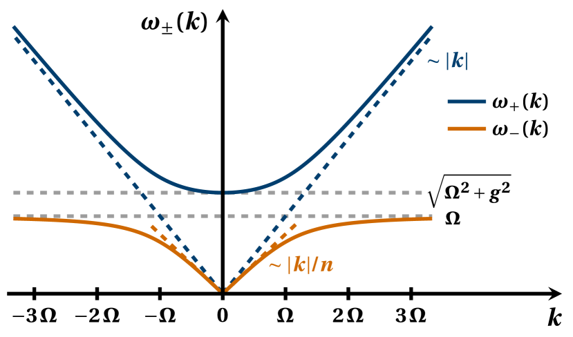
Figure 2: Plot of the dispersion relation $\omega_{\pm}(k)$ in Eq. (20) with exemplary parameters $g/\Omega=5/6$.

V Particle creation

Based on the model established above, one may study various quantum effects in and out of equilibrium. Since providing an ab initio treatment of time-dependent dissipative media is one of the major benefits our approach offers compared to existing models, we will henceforth focus on non-equilibrium phenomena. In principle, one could consider time-dependent parameters $\Omega(t)$, $g(t)$, or $G(t)$; or a combination of them. In order to illustrate the novel features of our model (in comparison to non-dissipative Hopfield dielectrics), let us consider a scenario where we switch on and off dissipation by a time-dependent $G(t)$ with $G(t\to\pm\infty)=0$ while the other two parameters $\Omega$ and $g$ are kept constant.

Even for constant $\Omega$ and $g$, solving the decoupled field equation (IV.1) is quite involved for general profiles $G(t)$, which makes it hard to reach progress analytically. A major difficulty arises from the interplay of excitation and dissipation, i.e., particles are already damped while they are created. In order to focus on the phenomenon of particle creation (and to separate it from the competing damping effect), we assume that the coupling $G(t)$ is switched on for a sufficiently short time and to a maximum value which is not too large, such that the damping during this switching time can be neglected in a first approximation.

V.1 Perturbation Theory

Formally, the approximation described above can be implemented via perturbation theory based on a power expansion in $G$. As one option, this can be formulated in the framework of time-dependent perturbation theory with the perturbation Hamiltonian $\hat{H}_{\Psi\Phi}$ stemming from the Lagrangian $L_{\Psi\Phi}$ given in Eq. (6), while the remaining contributions $L_{A}+L_{\Psi}+L_{A\Psi}+L_{\Phi}$ correspond to the undisturbed $\hat{H}_{0}$ problem. As another option, we may approximate the equations of motion for the field operators by omitting all terms of order ${\cal O}(G^{2})$. Decoupling the original problems (7), (8) and (9) for time-dependent $G(t)$ in this way yields the simplified expression

$$\left[\left(\partial_{t}^{2}+\Omega^{2}\right)\left(\partial_{t}^{2}-\partial_{x}^{2}\right)+g^{2}\partial_{t}^{2}\right]\hat{A}(t,x)=\qquad\quad$$

$$-g\partial_{t}G(t)\partial_{t}\hat{\Phi}_{0}(t,x,y=0)+{\cal O}(G^{2})\,,\quad$$ (23)

see also Eq. (III.1). After inserting the inhomogeneity (18), comparing the initial $\hat{A}^{\rm in}(t,x)$ and final $\hat{A}^{\rm out}(t,x)$ solutions (both expressed in terms of the creation and annihilation operators introduced in Sec. IV.2) yields the Bogoliubov transformation (to first order in $G$)

$$\hat{a}_{\pm}^{\rm out}(k)=\hat{a}_{\pm}^{\rm in}(k)+\int d\kappa\left(\alpha_{k\kappa}^{\pm}\hat{b}_{k\kappa}+\beta_{k\kappa}^{\pm}\hat{b}_{-k\kappa}^{\dagger}\right)\,.$$ (24)

The Bogoliubov coefficients $\alpha_{k\kappa}^{\pm}$ and $\beta_{k\kappa}^{\pm}$ connecting the initial $\hat{a}_{\pm}^{\rm in}(k)$ and final $\hat{a}_{\pm}^{\rm out}(k)$ annihilation operators (i.e., before and after switching on an off dissipation) with the initial environment operators $\hat{b}_{k\kappa}$ and $\hat{b}_{k\kappa}^{\dagger}$ are proportional to the Fourier transform $\widetilde{G}(\omega)$ of the switching function $G(t)$, evaluated at $\omega_{\pm}(k)-|\kappa|$ and $\omega_{\pm}(k)+|\kappa|$, respectively, plus ${\cal O}(G^{2})$ corrections.

To lowest order in $G$, the number (density) of particles created per unit length is given by

$$\langle\hat{n}_{\pm}^{\rm out}(k)\rangle_{\rm in} = \int d\kappa\,\left|\beta_{k\kappa}^{\pm}\right|^{2}=\frac{\rho(k)\mp\sigma(k)}{8\rho(k)\omega_{\pm}(k)}\int d\kappa\,|\kappa|\,\times$$ (25)

$$\times\left|\widetilde{G}\left(\omega_{\pm}(k)+|\kappa|\right)\right|^{2}\,.$$

Assuming that the characteristic rate of change in the switching function $G(t)$ is much slower than the medium frequency $\Omega$, the number $\langle\hat{n}_{+}^{\rm out}(k)\rangle_{\rm in}$ of particles in the upper band $\omega_{+}(k)$ is exponentially suppressed due to $\omega_{+}(k)\geq\sqrt{\Omega^{2}+g^{2}}$. For the same reason, we may approximate the lower band according to $\omega_{-}(k)\approx|k|/n$ .

V.2 Lorentzian Profile

A particularly simple expression can be obtained for a switching function in the form of a Lorentz pulse

$$G(t)=G_{0}\frac{\tau^{2}}{\tau^{2}+t^{2}}\,,$$ (26)

with the characteristic switching time $\tau>0$. In this case, the Fourier transform is just an exponential function $\widetilde{G}(\omega)=G_{0}\tau\sqrt{\pi/2}\exp\{-\tau|\omega|\}$ and the total number of created particles $N$ per length $\ell$ reads

$$\frac{N}{\ell}\approx\frac{1}{32}\,\frac{g^{2}}{\sqrt{\Omega^{2}+g^{2}}}\,\frac{G_{0}^{2}}{\Omega^{3}\tau^{2}}=\frac{\Gamma_{0}}{(\Omega\tau)^{2}}\,\frac{n^{2}-1}{8n}\,.$$ (27)

Since we have assumed a slow switching function, i.e., $\Omega\tau\gg 1$, a significant number $N$ of photons can only be created by switching the dissipation in a region of sufficiently large optical path length $n\ell$. Even though the above result was obtained for the specific switching function (26), the qualitative scaling behavior should be the same for other (reasonable) profiles $G(t)$.

Let us compare the above number to the well-known case of changing the refractive index $n(t)$ by a small amount $\Delta n\ll 1$ in absence of dissipation, see, e.g., [20, 35, 33, 34]. For a Lorentzian perturbation $\Delta n(t)$ analogous to Eq. (26), the number of particles $N$ per unit length $\ell$ reads

$$\frac{N}{\ell}=\frac{\pi}{16}\,\frac{(\Delta n)^{2}}{n\tau}\,.$$ (28)

In non-linear dielectric media, refractive index perturbations $\Delta n(t)$ of order ${\cal O}(10^{-3})$ can be generated by strong laser pulses and the Kerr effect [18, 59]. Slightly stronger perturbations $\Delta n(t)$ of order ${\cal O}(10^{-2})$ have been reported for tunable meta-materials [31]. However, since the number of created particles $N/\ell$ is of second order in $\Delta n$, switching dissipation could be more effective.

V.3 Partner Particles

As is well known, changing the refractive index $n(t)$ creates photons in pairs with opposite momenta $\pm k$. The relation between photons and their partners can be observed in the two-point correlation function $\langle\hat{A}(t,x)\hat{A}(t,x^{\prime})\rangle$, for example. For times $t$ long after the switch, one obtains distinctive signatures at distances $|x-x^{\prime}|=2t/n+{\cal O}(\tau)$, see also [60, 34].

In contrast, the partners of photons created by switching on and off dissipation are not other medium photons, but excitations of the environment field $\Phi$. This can already be inferred from the (lowest-order) Bogoliubov transformation (24), see [61]. As another signature, we find pairs of peaks in the correlation function $\langle\hat{\Phi}(t,x,y)\hat{A}(t,x^{\prime})\rangle$ at distances $|y|=t+{\cal O}(\tau)$ and $|x-x^{\prime}|=t/n+{\cal O}(\tau)$, but not (to first order) in the correlation $\langle\hat{A}(t,x)\hat{A}(t,x^{\prime})\rangle$.

Apart from this, there is no first-order imprint in the two-point function $\langle\hat{\Phi}(t,x,y)\hat{\Phi}(t,x^{\prime},y^{\prime})\rangle$, which indicates again that all excitations created in the $\Phi$ field have partners in the medium. Therefore, we obtain no pairs of correlated $\Phi$ excitations (to lowest order), in contrast to another mechanism of quantum radiation studied in Ref. [53], where both partners eventually escape to a surrounding field.

V.4 Sudden Switching

Previous works including Refs. [53, 56] have simplified their analysis by considering scenarios in which the light-matter coupling is suddenly switched off. This simplification is not necessary in our approach, which allows us to take into account the dependence on the temporal switching function $G(t)$. For a step-like profile $G(t)=G_{0}\Theta(-t)$, our perturbative result (25) yields divergent particle numbers $\langle\hat{n}_{\pm}^{\rm out}(k)\rangle_{\rm in}$ for all modes $k$. This singularity is caused by an ultra-violet (UV) divergence of the $\kappa$-integration and stems from the idealized interaction term $L_{\Psi\Phi}$ in our model Lagrangian (1) which has no UV cutoff and thus couples each mode $k$ of the medium to arbitrarily large wave numbers $\kappa$ of the environment $\Phi$. By analytically solving Eq. (IV.1) in case of $G(t)=G_{0}\Theta(-t)$ with constant $\Omega$ and $g$, we have found this result to apply even beyond the scope of perturbation theory.

VI Conclusions

We generalized the well-known Hopfield model involving the electromagnetic field $A$ and the medium polarization field $\Psi$ by adding an environment field $\Phi$. In this way, we arrived at a microscopic Lagrangian corresponding to a 1+1 dimensional dielectric medium including dispersion and dissipation. The model is constructed in such a way that it allows for the derivation of quantum electrodynamics in such media without ambiguities and without resorting to additional assumptions such as the Markov approximation. Consequently, it naturally accounts for the dynamics in media with time-dependent backgrounds, which is a major benefit in comparison to existing models for dissipative dielectrics.

As an exemplary configuration with non-constant parameters, we considered switching on and off dissipation and derived the number of created photons in dependence on the temporal switching function $G(t)$ and the switching time $\tau$. To further illustrate the photon yield calculated above, let us compare two scenarios: In scenario I, we consider a Lorentzian pulse $G(t)$ of height $G_{0}$ and width $\tau$ within a time-dependent waveguide of length $\ell$. In scenario II, we envision a static waveguide of the same length $\ell$ with constant coupling $G_{0}$ (see Sec. III.1). Now, if $\ell$ (for a given $G_{0}$) was sufficiently large that typical photons of frequencies $\omega={\cal O}(1/\tau)$ would be damped away according to Eqs. (15) and (16) before fully traversing the static waveguide in scenario II, the corresponding scenario I (with the same $G_{0}$) would yield a particle number of order unity. As we switch dissipation just briefly to the strength $G_{0}$, most particles created by the modulation $G(t)$ are not dissipated but should, in principle, be observable after dissipation has been switched off again. Thus, the photon yield of a short pulse $G(t)$ could exceed the quantum radiation generated by a time-dependent refractive index $n(t)$, because variations $\Delta n(t)$ are typically small and yield photon numbers quadratic in $\Delta n$.

Since quantum radiation typically creates particles in pairs (i.e., a squeezed state), another interesting question concerns the partner particles of the produced photons. In contrast to the case of a time-dependent refractive index $n(t)$ and other scenarios (see, e.g., [53, 54, 55]), we find that the partner particles of photons created by switching on and off dissipation are (primarily) excitations of the environment field $\Phi$ instead of other photons.