When Explanations Lie: Why Many Modified BP Attributions Fail

Abstract

Attribution methods aim to explain a neural network’s prediction by highlighting the most relevant image areas. A popular approach is to backpropagate (BP) a custom relevance score using modified rules, rather than the gradient. We analyze an extensive set of modified BP methods: Deep Taylor Decomposition, Layer-wise Relevance Propagation (LRP), Excitation BP, PatternAttribution, DeepLIFT, Deconv, RectGrad, and Guided BP. We find empirically that the explanations of all mentioned methods, except for DeepLIFT, are independent of the parameters of later layers. We provide theoretical insights for this surprising behavior and also analyze why DeepLIFT does not suffer from this limitation. Empirically, we measure how information of later layers is ignored by using our new metric, cosine similarity convergence (CSC). The paper provides a framework to assess the faithfulness of new and existing modified BP methods theoretically and empirically.

1 Introduction

Explainable AI (XAI) aims to improve the interpretability of machine learning models. For deep convolutional networks, attribution methods visualize the areas relevant for the prediction with so-called saliency maps. Various attribution methods have been proposed, but do they reflect the model behavior correctly?

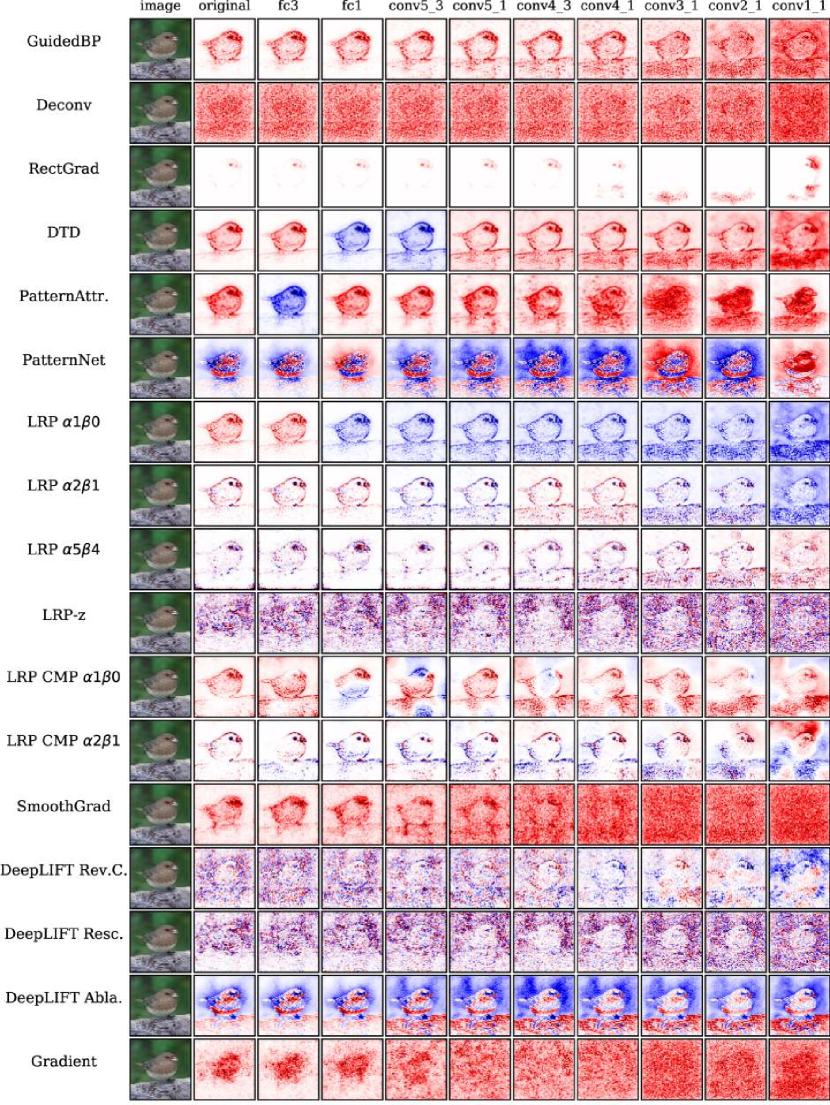
(Adebayo et al., 2018) proposed a sanity check: if the parameters of the model are randomized and therefore the network output changes, do the saliency maps change too? Surprisingly, the saliency maps of GuidedBP (Springenberg et al., 2014) stay identical, when the last layer (fc3) is randomized (see Figure 1(a)). A method ignoring the last layer can not explain the network’s prediction faithfully.

(a) Sanity Checks (VGG-16)

(b) Image

(c) Expl. Cat

(d) Expl. Dog

(e) Diff. (c) - (d)

Figure 1: (a) Sanity Checks: Saliency maps should change if network parameters are randomized. Parameters are randomized from the last to the first layer. Red denotes positive and blue negative relevance. (b-e) Class insensitivity of LRP_α1β0 on VGG-16. Explanation for (c) Persian cat (283) and (d) King Charles Spaniel (156). (e) Difference (c) - (d), both normalized to $[0,1]$. L1-norm of (e) = 0.000371.

In addition to (Adebayo et al., 2018), which only reported GuidedBP to fail, we found several modified backpropagation (BP) methods fail too: Layer-wise Relevance Propagation (LRP), Deep Taylor Decomposition (DTD), PatternAttribution, Excitation BP, Deconv, GuidedBP, and RectGrad (Bach et al., 2015; Montavon et al., 2017; Kindermans et al., 2018; Zhang et al., 2018; Zeiler & Fergus, 2014; Springenberg et al., 2014; Kim et al., 2019). The only tested modified BP method passing is DeepLIFT (Shrikumar et al., 2017).

Modified BP methods estimate relevant areas by backpropagating a custom relevance score instead of the gradient. For example, DTD only backpropagates positive relevance scores. Modified BP methods are popular with practitioners (Yang et al., 2018; Sturm et al., 2016; Eitel et al., 2019). For example, (Schiller et al., 2019) uses saliency maps to improve the classification of whale sounds or (Böhle et al., 2019) use LRP_α1β0 to localize evidence for Alzheimer’s disease in brain MRIs.

Deep neural networks are composed of linear layers (dense, conv.) and non-linear activations. For each linear layer, the weight vector reflects the importance of each input directly. (Bach et al., 2015; Kindermans et al., 2018; Montavon et al., 2017) argue that aggregating explanations of each linear model can explain a a deep neural network. Why do these methods then fail the sanity check?

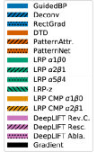
Theoretically, we show that the $z^{+}$-rule – used by DTD, LRP_α1β0, and Excitation BP – yields a multiplication chain of non-negative matrices. Each matrix corresponds to a layer. The saliency map is a function of this matrix chain. We show that such a non-negative matrix chain converges to a rank-1 matrix. If $C\!\in\!\mathbb{R}^{n\times m}$ is a rank-1 matrix, then it can be written as an outer product $C\!=\!{\bm{c}}\bm{\gamma}^{T},\ {\bm{c}}\!\in\!\mathbb{R}^{n}$, $\bm{\gamma}\!\in\!\mathbb{R}^{m}$. Multiplying $C$ with any vector ${\bm{v}}$ yields always the same the direction: $C{\bm{v}}={\bm{c}}\bm{\gamma}^{T}{\bm{v}}=\!\lambda{\bm{c}},\lambda\!\in\!\mathbb{R}$. The scaling is irrelevant as saliency maps are normalized. If sufficiently converged, the backpropagated vector can merely switch the sign of the saliency map. For example, in Figure 1(a), the sign of the PatternAttribution saliency map switches due to the randomization of fc3. Figure 1(b)-1(e) show how the saliency maps of LRP_α1β0 become class-insensitive.

Empirically, we quantify the convergence to a rank-1 matrix using our novel cosine similarity convergence (CSC) metric. CSC allows to retrace, layer by layer, how modified BP methods lose information about previous layers. Using CSC, we observe that all analyzed modified BP methods, except for DeepLIFT, converge towards a rank-1 matrix on VGG-16 and ResNet-50. For sufficiently large values of $\alpha$ and $\beta$, LRP_αβ does not converge but also produces rather noisy saliency maps.

The paper focuses on modified BP methods, as other attribution methods do not suffer from the converges problem. They either rely on the gradient directly (Smilkov et al., 2017; Sundararajan et al., 2017), which does not converge or consider the model as a black-box (Ribeiro et al., 2016; Lundberg & Lee, 2017).

Our findings show that many modified BP methods are prone to class-insensitive explanations and provide saliency maps that rather highlight low-level features. Negative relevance scores are crucial to avoid the convergence to a rank-1 matrix — a possible future research direction.

2 Theoretical Analysis

Notation

For our theoretical analysis, we consider feed-forward neural networks with a ReLU activation function $[{\bm{x}}]^{+}=\max(0,{\bm{x}})$. The neural network $f({\bm{x}})$ contains $n$ layers, each with weight matrices $W_{l}$. The output of the $l$-th layer is denoted by ${\bm{h}}_{l}$. We use ${[ij]}$ to index the $i,j$ element in $W_{l}$ as in $W_{l_{[ij]}}$. To simplify notation, we absorb the bias terms into the weight matrix, and we omit the final softmax layer. We refer to the input with ${\bm{h}}_{0}={\bm{x}}$ and to the output with ${\bm{h}}_{n}=f({\bm{x}})$. The output of the $l$-th layer is given by:

$${\bm{h}}_{l}=[W_{l}{\bm{h}}_{l-1}]^{+}$$ (1)

All the results apply to convolutional neural networks as convolution can be expressed as matrix multiplication.

Gradient

The gradient of the $k$-th output of the neural network w.r.t. the input ${\bm{x}}$ is given by:

$$\frac{\partial f_{k}({\bm{x}})}{\partial{\bm{x}}}=W_{1}^{T}M_{1}\frac{\partial f_{k}({\bm{x}})}{\partial{\bm{h}}_{1}}=\prod_{l}^{n}\left(W_{l}^{T}M_{l}\right)\cdot{\bm{v}}_{k},$$ (2)

where $M_{l}=\operatorname{diag}(1_{h_{l}>0})$ denotes the gradient mask of the ReLU operation. The last equality follows from recursive expansion. The vector ${\bm{v}}_{k}$ is a one-hot vector to select the $k$-th output.

The gradient of residual blocks is also a product of matrices. The gradient of ${\bm{h}}_{l+1}={\bm{h}}_{l}+g({\bm{h}}_{l})$ is:

$$\frac{\partial{\bm{h}}_{l+1}}{\partial{\bm{h}}_{l}}=I+G_{\partial g({\bm{h}}_{l})/\partial{\bm{h}}_{l}},$$ (3)

where $G_{\partial g({\bm{h}}_{l})/\partial{\bm{h}}_{l}}$ denotes the derivation matrix of the residual block, and $I$ is the identity matrix. For the gradient, the final saliency map is usually obtained by summing the absolute channel values of the relevance vector $r^{\nabla}_{0}({\bm{x}})$ of the input layer.

The following methods modify the gradient definition and to distinguish the rules, we introduce the notation: $r_{l}^{\nabla}({\bm{x}})=\frac{\partial f({\bm{x}})}{\partial{\bm{h}}_{l}}$ which denotes the relevance at layer $l$ for an input ${\bm{x}}$.

Interpretability of Linear Models

The relevance of the input of a linear model can be calculated directly. Let $y={\bm{w}}^{T}{\bm{x}}$ be a linear model with a single output scalar. The relevance of the input ${\bm{x}}$ to the $i$-th output ${\bm{y}}_{[i]}$ is :

$$r_{\bm{x}}^{\text{Linear}}({\bm{x}})={\bm{w}}\odot{\bm{x}}.$$ (4)

2.1 $z^{+}$-Rule

The $z^{+}$-rule is used by DTD (Montavon et al., 2017), Excitation BP (Zhang et al., 2018) and also corresponds to the LRP_α1β0  rule (Bach et al., 2015). The $z^{+}$-rule backpropagates positive relevance values, which are supposed to correspond to the positive evidence for the prediction. Let $w_{ij}$ be an entry in the weight matrix $W_{l}$:

$$\begin{split}r_{l}^{z^{+}}({\bm{x}})&=Z^{+}_{l}\cdot r_{l+1}^{z^{+}}({\bm{x}})\\ \text{where}\,Z_{l}^{+^{T}}&=\left(\frac{[w_{ij}{\bm{h}}_{l_{[j]}}]^{+}}{\sum_{k}[w_{ik}{\bm{h}}_{l_{[k]}}]^{+}}\right)_{[ij]}\end{split}$$ (5)

Each entry in the derivation matrix $Z^{+}_{l}$ is obtained by measuring the positive contribution of the input neuron $i$ to the output neuron $j$ and normalizing by the total contributions to neuron $j$. The relevance from the previous layer $r_{l+1}^{z^{+}}$ is then distributed according to $Z^{+}_{l}$. The relevance function $r_{l}^{z^{+}}:\mathbb{R}^{n}\mapsto\mathbb{R}^{m}$ maps input ${\bm{x}}$ to a relevance vector of layer $l$. For the final layer the relevance is set to the value of the explained logit value, i.e. $r_{n}^{z^{+}}({\bm{x}})=f_{k}({\bm{x}})$. In contrast to the vanilla backpropagation, algorithms using the $z^{+}$-rule do not apply a mask for the ReLU activation.

The relevance of multiple layers is computed by applying the $z^{+}$-rule to each of them. Similar to the gradient, we obtain a product of non-negative matrices: $C_{k}=\prod^{k}_{l}Z^{+}_{l}$.

Theorem 1.

Let $A_{1},A_{2},A_{3}\dots$ be a sequence of non-negative matrices for which $\lim_{n\to\infty}A_{n}$ exists. We exclude the cases where one column of $\lim_{n\to\infty}A_{n}$ is the zero vector or two columns are orthogonal to each other. Then the product of all terms of the sequence converges to a rank-1 matrix $\bar{C}$:

$$\bar{C}:=\prod_{i=1}^{\infty}A_{i}=\bar{\bm{c}}\bm{\gamma}^{T}\,.$$ (6)

(Hajnal, 1976; Friedland, 2006) proved a similar result for squared matrices. In appendix A, we provide a rigorous proof of the theorem using the cosine similarity.

Figure 2: The positive column vectors ${\bm{a}}_{1},{\bm{a}}_{2}$ of matrix $A_{1}$ (orange) form a cone. The resulting columns of $A_{1}A_{2}$ (green) are contained in the cone as they are positive linear combinations of ${\bm{a}}_{1},{\bm{a}}_{2}$. At each iteration, the cone shrinks.

The geometric intuition of the proof is depicted in Figure 2. The column vectors of the first matrix are all non-negative and therefore in the positive quadrant. For the matrix multiplication $A_{i}A_{j}$, observe that $A_{i}{\bm{a}}_{k}$ is a non-negative linear combination of the column vectors of $A_{i}$, where ${\bm{a}}_{k}$ is the $k$-th column vector $A_{j_{[:k]}}$. The result will remain in the convex cone of the column vectors of $A_{i}$. The conditions stated in the theorem ensure that the cone shrinks with every iteration and it converges towards a single vector. In the appendix B, we simulate different matrix properties and find non-negative matrices to converge exponentially fast.

The column vectors of a rank-1 matrix are linearly dependent $C\!=\!{\bm{c}}\bm{\gamma}^{T}$. A rank-1 matrix $C$ always gives the same direction of ${\bm{c}}$: $CZ^{+}_{k+1}\!=\!{\bm{c}}\bm{\gamma}^{T}Z^{+}_{k+1}\!=\!{\bm{c}}\bm{\lambda}^{T}$ and for any vector ${\bm{v}}$: $CZ^{+}_{k+1}{\bm{v}}={\bm{c}}\bm{\lambda}^{T}{\bm{v}}=t{\bm{c}}$, where $t\in\mathbb{R}$. For a finite number of matrices $C_{k}=\prod^{k}_{l}Z^{+}_{l}$, $C_{k}$ might resemble a rank-1 matrix up to floating-point imprecision or $C_{k}Z^{+}_{k+1}$ might still be able to alter the direction. In any case, the influence of later matrices decreases.

The $Z^{+}$ matrices of dense layers fulfill the conditions of theorem 1. Convolutions can be written as matrix multiplications. For 1x1 convolutions, the kernels do not overlap and the row vectors corresponding to each location are orthogonal. In this case, the convergence happens only locally per feature map location. For convolutions with overlapping kernels, the global convergence is slower than for dense layers. In a ResNet-50 where the last convolutional stack has a size of (7x7), the overlapping of multiple (3x3) convolutions still induces a considerable global convergence (see LRP_CMP on ResNet-50 in section 5).

If an attribution method converges, the contributions of the layers shrink by depth. In the worst-case scenario, when converged up to floating-point imprecision, the last layer can only change the scaling of the saliency map. However, the last layer is responsible for the network’s final prediction.

2.2 Modified BP algorithms

LRP_z

The LRP_z rule of Layer-wise Relevance Propagation modifies the backpropagation rule as follows:

$$\begin{split}r_{l}^{z-\text{LRP}}({\bm{x}})&=Z_{l}\cdot r_{l+1}^{z-\text{LRP}}({\bm{x}}),\\ \text{where}\,Z_{l}&=\left(\frac{w_{ij}{\bm{h}}_{l_{[j]}}}{\sum_{k}w_{ik}{\bm{h}}_{l_{[k]}}}\right)_{[ij]}^{T}.\end{split}$$ (7)

If only max-pooling, linear layers, and ReLU activations are used, it was shown that LRP_z corresponds to gradient$\odot$input, i.e. $r_{0}^{z-\text{LRP}}({\bm{x}})={\bm{x}}\odot\frac{\partial f({\bm{x}})}{\partial{\bm{x}}}$ (Shrikumar et al., 2016; Kindermans et al., 2016; Ancona et al., 2017). LRP_z can be considered a gradient-based and not a modified BP method. The gradient is not converging to a rank-1 matrix and therefore gradient$\odot$input is also not converging.

(a) PatternNet

(b) $W=U_{l}\Sigma_{l}V_{l}$

(c) $T_{l}=\sqrt{\Sigma_{l}}V_{l}U_{l+1}\sqrt{\Sigma_{l+1}}$

Figure 3: PatternNet & PatternAttr.: (a)(b) Ratio between the first and second singular value $\sigma_{1}/\sigma_{2}$ for $A_{l},W_{l},$ and $A_{l}\odot W_{l}$. (c) $\sigma_{1}/\sigma_{2}$ of inter-layer derivation matrices. For (b) (c), we sliced the 3x3 convolutional kernels to 1x1 kernels.

LRP_αβ

separates the positive and negative influences:

$$r_{l}^{\alpha\beta}({\bm{x}})=\left(\alpha{Z}_{l}^{+}-\beta Z_{l}^{-}\right)r_{l+1}^{\alpha\beta}({\bm{x}}),$$ (8)

where $Z_{l}^{+}$ and $Z_{l}^{-}$ correspond to the positive and negative entries of the matrix $Z$. (Bach et al., 2015) propose to weight positives more: $\alpha\geq 1$ and $\alpha-\beta=1$. For LRP_α1β0, this rule corresponds to the $z^{+}$-rule, which converges. For $\alpha>1$ and $\beta>0$, the matrix $Z_{l}=\alpha{Z}_{l}^{+}-\beta Z_{l}^{-}$ can contain negative entries. Our empirical results show that LRP_αβ still converges for the most commonly used parameters $\alpha=2,\beta=1$ and even for a higher $\alpha=5$ it converges considerable on the ResNet-50.

Deep Taylor Decomposition

uses the $z^{+}$-rule if the input to a convolutional or dense layer is in $[0,\infty]$, i.e. if the layer follows a ReLU activation. For inputs in $\mathbb{R}$, DTD also proposed the $w^{2}$-rule and the so-call $w^{\mathcal{B}}$ rule for bounded inputs. Both rules were specifically designed to produce non-negative outputs. Theorem 1 applies and DTD converges to a rank-1 matrix necessarily.

PatternNet & PatternAttribution

takes into account that the input ${\bm{h}}_{l}$ contains noise. If ${\bm{d}}_{l}$ corresponds to the noise and ${\bm{s}}_{l}$ to the signal, than ${\bm{h}}_{l}={\bm{s}}_{l}+{\bm{d}}_{l}$. To assign the relevance towards the signal direction, it is estimated using the following equation:

$${\bm{a}}_{i}=\frac{\operatorname{cov}[{\bm{h}}]{\bm{w}}_{i}}{{\bm{w}}^{T}_{i}\operatorname{cov}[{\bm{h}}]{\bm{w}}_{i}},$$ (9)

where $a_{i}$ is the estimated signal direction for the $i-th$ neuron with input ${\bm{h}}$ and weight vector ${\bm{w}}_{i}=W_{[i:]}$. PatternNet is designed to recover the relevant signal in the data. Let $A_{l{[i:]}}={\bm{a}}_{i}$ be the corresponding signal matrix to the weight matrix $W_{l}$, the rule for PatternNet is:

$$r_{l}^{\text{PN}}({\bm{x}})=A_{l}^{T}\cdot r_{l+1}^{\text{PN}}({\bm{x}}),$$ (10)

PatternNet is also prone to converge to a rank-1 matrix. To recover the relevant signal, it might be even desired to converge to the a single direction – the signal direction.

The convergence of PatternNet follows from the computation of the pattern vectors ${\bm{a}}_{i}$ in equation 9. It is similar to a single step of the power iteration method ${\bm{v}}_{k+1}=C{\bm{v}}_{k}/\left\lVert C{\bm{v}}_{k}\right\rVert$. In appendix C, we provide details on the relationship to power iteration and also derive equation 9 from the equation given in (Kindermans et al., 2018). The power iteration method converges to the eigenvector with the largest eigenvalue exponentially fast.

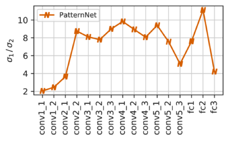
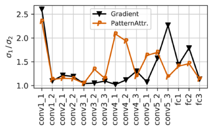
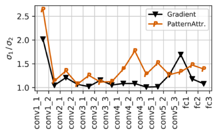
All column vectors in $A_{[i:]}={\bm{a}}_{i}$ underwent a single step of the power iteration and therefore tend to point towards the first eigenvector of $\operatorname{cov}[{\bm{h}}]$. This can also be verified empirically: the ratio of the first and second singular value $\sigma_{1}(A)/\sigma_{2}(A)>6$ for almost all the VGG-16 patterns (see Figure 3(a)), indicating a strong convergence of the matrix chain towards a single direction.

The findings from PatternNet are hard to transfer to PatternAttribution. The rule for PatternAttribution uses the Hadamard product of $A_{l}$ and $W_{l}$:

$$r_{l}^{\text{PA}}({\bm{x}})=\left(W_{l}\odot A_{l}\right)^{T}\cdot r_{l+1}^{\text{PA}}({\bm{x}}),$$ (11)

The Hadamard product complicates any analytic argument using the properties of $A_{l}$ or $W_{l}$. The theoretical results available (Ando et al., 1987; Zhan, 1997) did not allow us to show that PatternAttribution converges to a rank-1 matrix necessarily.

We provide a mix of theoretical and empirical insights on why it converges. The conditions of convergence can be studied well on the singular value decomposition: $(W_{l}\odot A_{l})^{T}=U_{l}\Sigma_{l}V_{l}$. Loosely speaking, the matrix chain will converge to a rank-1 matrix if the first $\sigma_{1}$ and second $\sigma_{2}$ singular values in $\Sigma_{l}$ differ and if $V_{l}$ and $U_{l+1}$ are aligned such that higher singular values of $\Sigma_{l}$ and $\Sigma_{l+1}$ are multiplied together such that the ratio $\sigma_{1}/\sigma_{2}$ grows.

To see how well the per layer matrices align, we look at the inter-layer chain members: $T_{l}=\sqrt{\Sigma_{l}}V_{l}U_{l+1}\sqrt{\Sigma_{l+1}}$. In Figure 3, we display the ratio between the first and second singular values $\sigma_{1}(T_{l})/\sigma_{2}(T_{l})$. For $W\odot A$, the first singular value is considerably larger than for the plain weights $W$. Interestingly, the singular value ratio of inter-layer matrices shrinks for the plain $W$ matrix. Whereas for PatternAttribution, the ratio increases for some layers indicating that the Hadamard product leads to more alignment of the matrices.

DeepLIFT

is the only tested modified BP method which does not converge to a rank-1 matrix. It is an extension of the backpropagation algorithm to finite differences:

$$\frac{f({\bm{x}})-f({\bm{x}}^{0})}{{\bm{x}}-{\bm{x}}^{0}}$$ (12)

For the gradient, one would take the limit ${\bm{x}}^{0}\to{\bm{x}}$. DeepLIFT uses a so-called reference point for ${\bm{x}}^{0}$ instead, such as zeros or for images a blurred version of ${\bm{x}}$. The finite differences are backpropagated, similar to infinitesimal differences. The final relevance is the difference in the $k$-th logit: $r^{DL}_{l}({\bm{x}})=f_{k}(x)-f_{k}(x^{0})$.

Additionally to the vanilla gradient, DeepLIFT separates positive and negative contributions. For ReLU activations, DeepLIFT uses either the RevealCancel or the Rescale rule. Please refer to (Shrikumar et al., 2017) for a description. The rule for linear layers is most interesting because it is the reason why DeepLIFT does not converge:

$$\begin{split}r^{DL+}_{l}({\bm{x}},{\bm{x}}^{0})=&M^{T}_{>0}\odot\left(W_{l}^{+^{T}}r^{DL+}_{l+1}({\bm{x}},{\bm{x}}^{0})\right.\\ &\left.+W_{l}^{-^{T}}r^{DL-}_{l+1}({\bm{x}},{\bm{x}}^{0})\vphantom{W_{l}^{-^{T}}}\right)\end{split}$$ (13)

where the mask $M_{>0}$ selects the weight rows corresponding to positive deltas ($0<\Delta{\bm{h}}_{l}={\bm{h}}_{l}-{\bm{h}}_{l}^{0}$). For negative relevance $r^{DL-}_{l}$, the rule is defined analogously. An interesting property of the rule (13) is that negative and positive relevance can influence each other.

If the intermixing is removed by only considering $W^{+}$ for the positive rule and $W^{-}$ for the negative rule, the two matrix chains become decoupled and converge. For the positive chain, this is clear. For the negative chain, observe that the multiplication of two non-positive matrices gives a non-negative matrix. Non-positive vectors ${\bm{b}},{\bm{c}}$ have an angle $\leq 90^{\circ}$ and ${\bm{c}}^{T}{\bm{b}}=\left\lVert{\bm{c}}\right\rVert\left\lVert{\bm{b}}\right\rVert\cos({\bm{c}},{\bm{b}})\geq 0$. In the evaluation, we included this variant as DeepLIFT Ablation, and as predicted by the theory, it converges.

Guided BP & Deconv & RectGrad

apply an additional ReLU to the gradient and it was shown to be invariant to the randomization of later layers previously in (Adebayo et al., 2018) and analyzed theoretically in (Nie et al., 2018):

$$r_{l}^{GBP}({\bm{x}})=W_{l}^{T}\left[M_{l}r_{l+1}^{GBP}({\bm{x}})\right]^{+}.$$ (14)

$M_{l}=\operatorname{diag}(1_{h_{1}>0})$ denotes the gradient mask of the ReLU operation. For Deconv, the mask of the forward ReLU is omitted, and the gradients are rectified directly. RectGrad (Kim et al., 2019) is related to GuidedBP and set the lowest $q$ percentile of the gradient to zero. As recommended in the paper, we used $q=98$.

As a ReLU operation is applied to the gradient, the backpropagation is no longer a linear function. The ReLU also results in a different failure than before. (Nie et al., 2018) provides a theoretical analysis for GuidedBP. Our results align with them.

3 Evaluation

(a) Random Logits

(b) Parameter Randomization

Figure 4: (a) SSIM between saliency maps explaining the ground-truth or a random logit. (b) The parameters of the VGG-16 are randomized, starting from the last to the first layer. SSIM quantifies the difference to the saliency map from the original model. Intervals show 99% bootstrap confidences.

Setup

We report results on a small network trained on CIFAR-10 (4x conv., 2x dense, see appendix D), a VGG-16 (Simonyan & Zisserman, 2014), and ResNet-50 (He et al., 2016). The last two are trained on the ImageNet dataset (Russakovsky et al., 2015), the standard dataset to evaluate attribution methods. The different networks cover different concepts: shallow vs. deep, forward vs. residual connections, multiple dense layers vs. a single one, using batch normalization. All results were computed on 200 images from the validation set. To justify the sample size, we show bootstrap confidence intervals in Figure 4(b) (Efron, 1979). We used the implementation from the innvestigate and deeplift package (Alber et al., 2019; Shrikumar et al., 2017) and added support for residual connections. The experiments were run on a single machine with two graphic cards and take about a day to complete.

Random Logit

We display the difference of saliency maps explaining the ground-truth and a random logit in Figure 4(a). As the logit value is responsible for the predicted class, the saliency maps should change. We use the SSIM metric (Wang et al., 2004) as in (Adebayo et al., 2018).

Sanity Check

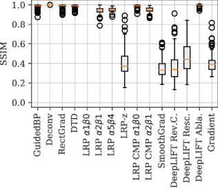
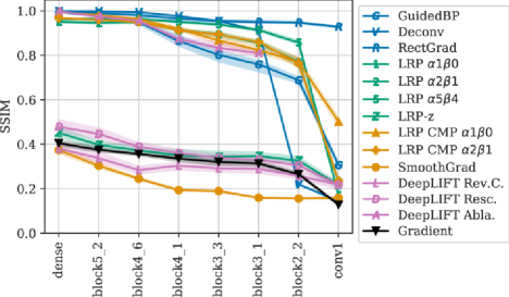
We followed (Adebayo et al., 2018) and randomized the parameters starting from the last layer to the first layer. For DTD and LRP_α1β0, randomizing the last layer flips the sign of the saliency map sometimes. We, therefore, compute the SSIM also between the inverted saliency map and report the maximum. In Figure 4(b), we report the SSIM between the saliency maps (see also Figure 1(a) and appendix G).

(a) ResNet-50

(b) VGG-16 (logarithmic)

(c) VGG-16 (linear)

(d) CIFAR-10

(e) VGG-16

(f) ResNet-50

(g) CIFAR10

Figure 5: (a)-(d) Median of the cosine similarity convergence (CSC) per layer between relevance vectors obtained from randomizing the relevance vectors of the final layer. (e)-(g) histogram of the distribution of the CSC after the first layer.

Cosine Similarity Convergence Metric (CSC)

Instead of randomizing the parameters, we randomize the backpropagated relevance vectors directly. We select layer $k$ and set the corresponding relevance to $r_{k}({\bm{x}}):={\bm{v}}_{1}$ where ${\bm{v}}_{1}\sim\mathcal{N}(0,I)$ and then backpropagate it as before. For example, for the gradient, we would do: $\frac{\partial h_{k}}{\partial h_{1}}\frac{\partial f(x)}{\partial h_{k}}:=\frac{\partial h_{k}}{\partial h_{1}}{\bm{v}}_{1}$. We use the notation $r_{l}({\bm{x}}|r_{k}\!:\!\leavevmode\resizebox{3.33333pt}{0.0pt}{=}{\bm{v}}_{1})$ to describe the relevance $r_{l}$ at layer $l$ when the relevance of layer $k$ is set to ${\bm{v}}_{1}$.

Using two random relevance vectors ${\bm{v}}_{1},{\bm{v}}_{2}\sim\mathcal{N}(0,I)$, we measure the convergence using the cosine similarity. A rank-1 matrix $C\!=\!{\bm{c}}\bm{\gamma}^{T}$ always yields the same direction: $C{\bm{v}}\!={\bm{c}}\bm{\gamma}^{T}\!=\!\lambda{\bm{c}}$. If the matrix chain converges, the backpropagated relevance vectors of ${\bm{v}}_{1},{\bm{v}}_{2}$ will align more and more. We quantify their alignment using the cosine similarity $s_{\cos}(r_{l}\left({\bm{x}}|r_{k}{:\leavevmode\resizebox{3.33333pt}{0.0pt}{=}}{\bm{v}}_{1}\right),r_{l}\left({\bm{x}}|r_{k}{:\leavevmode\resizebox{3.33333pt}{0.0pt}{=}}{\bm{v}}_{2}\right)))$ where $s_{\cos}({\bm{a}},{\bm{b}})={\bm{a}}^{T}{\bm{b}}\ /\ \left(\left\lVert{\bm{a}}\right\rVert\cdot\left\lVert{\bm{b}}\right\rVert\right)$.

Suppose the relevance matrix chain would converge to a rank-1 matrix perfectly, than we have for both ${\bm{v}}_{1},{\bm{v}}_{2}$: $r_{l}({\bm{x}}|r_{k}\leavevmode\resizebox{3.33333pt}{0.0pt}{=}{\bm{v}}_{i})=C{\bm{v}}_{i}=c\bm{\gamma}^{T}{\bm{v}}_{i}=\lambda_{i}{\bm{c}}$ where $\lambda_{i}=\bm{\gamma}^{T}{\bm{v}}_{i}$ and their cosine similarity will be one. The opposite direction is also true. If $C$ has shape $n\times m$ with $n\leq m$ and if for $n$ linearly independent vectors ${\bm{v}}_{i}$, the cosine similarity $s_{\cos}(C{\bm{v}}_{i},C{\bm{v}}_{j})=1$, then $C$ is a rank-1 matrix.

An alternative way to measure convergence would have been to construct the derivation matrix $C_{k}=\prod^{k}_{l=1}Z_{l}$ and measure the ratio $\sigma_{1}(C_{k})/\sigma_{2}(C_{k})$ of the first to the second-largest singular value of $C_{k}$. Although this approach is well motivated theoretically, it has some performance downsides. $C_{k}$ would be large and computing the singular values costly.

We use five different random vectors per sample – in total 1000 convergence paths. As the vectors are sampled randomly, it is unlikely to miss a region of non-convergence (Bergstra & Bengio, 2012).

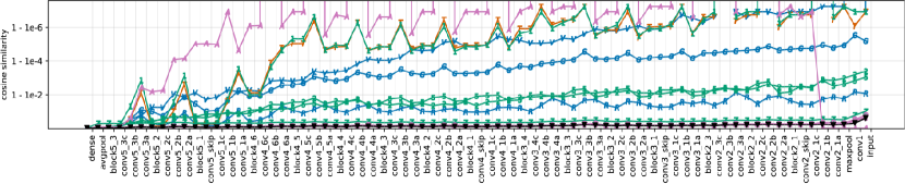
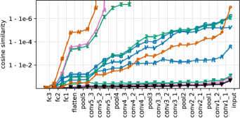
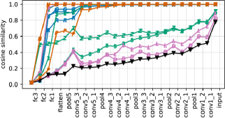
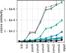
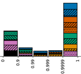
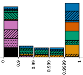
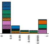
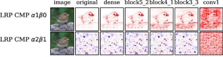
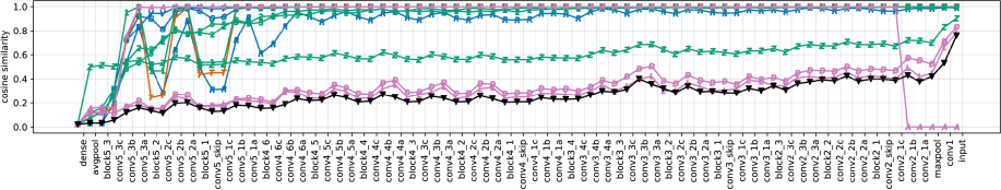
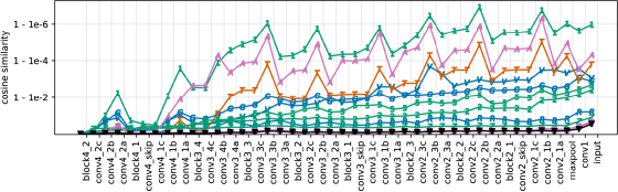
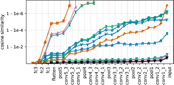
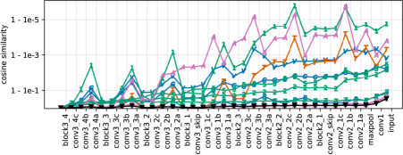
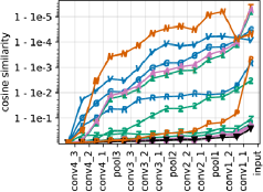
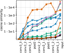
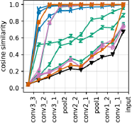
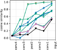
For convolution layers, we compute the cosine similarity per feature map location. For a shape of $(h,w,c)$, we obtain $h\cdot w$ values. The jump in cosine similarity for the input is a result of the input’s low dimension of 3 channels. In Figure 5, we plot the median cosine similarity for different networks and attribution methods (see appendix F for additional Figures). We also report the histogram of the CSC at the first convolutional layer in Figures 5(e)-5(g).

4 Results

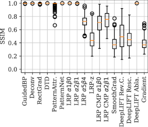
Our random logit analysis reveals that converging methods produce almost identical saliency maps, independently of the output logit (SSIM very close to 1). The rest of the field (SSIM between 0.4 and 0.8) produces saliency maps different from the ground-truth logit’s map (see Figure 4(a)).

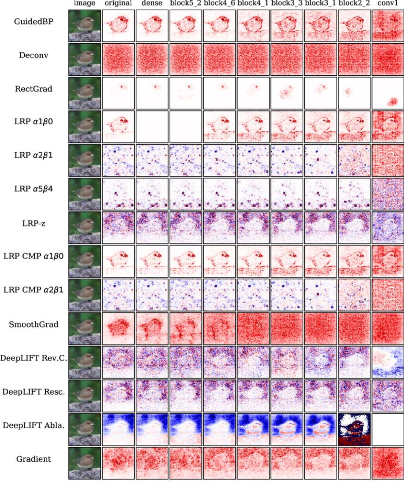
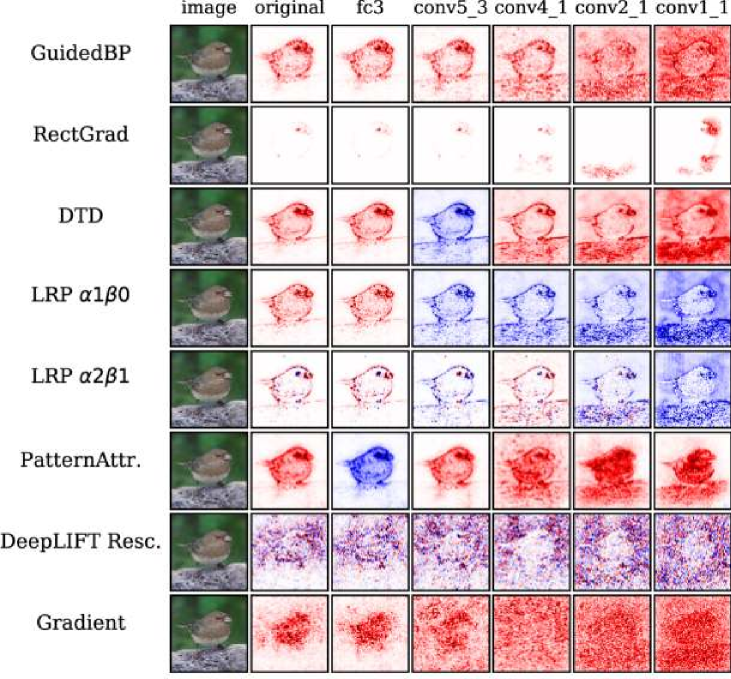
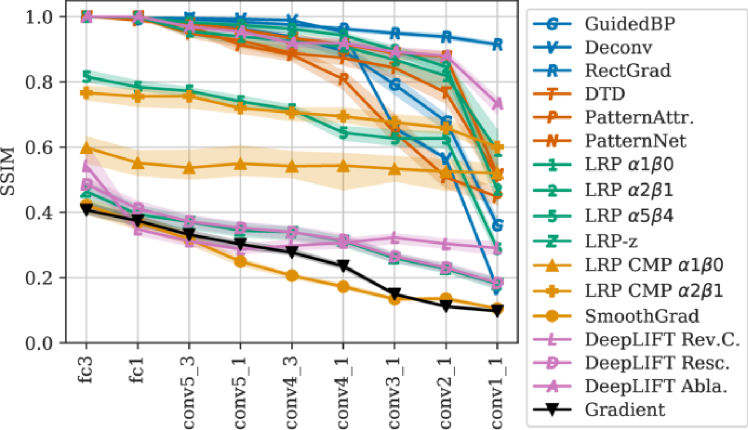
We observe the same distribution in the sanity check results (see Figure 4(b)). One group of methods produces similar saliency maps even when convolutional layers are randomized (SSIM close to 1). Again, the rest of the field is sensitive to parameter randomization. The same clustering can be observed for ResNet-50 (appendix E, Figure 8).

Our CSC analysis confirms that random relevance vectors align throughout the backpropagation steps (see Figure 5). Except for LRP_z and DeepLIFT, all methods show convergence up to at least 0.99 cosine similarity. LRP_α5β4 converges less strongly for VGG-16. Among the converging methods, the rate of convergence varies. LRP_α1β0, PatternNet, the ablation of DeepLIFT converges fastest. PatternAttribution has a slower convergence rate – still exponential. For DeepLIFT Ablation, numerical instabilities result in a cosine similarity of 0 for the first layers of the ResNet-50. Even on the small 6-layer network, the median CSC is greater than 1-1e-6 for LRP_α1β0 (see Figure 5(d)).

5 Discussion

When many modified BP methods do not explain the network faithfully, why was this not widely noticed before? First, it is easy to blame the network for unreasonable explanations – no ground truth exists. Second, MNIST, CIFAR, and ImageNet contain only a single object class per image – not revealing the class insensitivity. Finally, it might not be too problematic for some applications if the saliency maps are independent of the later network’s layers. For example, to explain Alzheimer’s disease (Böhle et al., 2019), local low-level features are sufficient as they are predictive for the disease and the data lacks conflicting evidences (i.e. the whole brain is affected).

When noticed, different ways to address the issue were proposed and an improved class sensitivity was reported (Kohlbrenner et al., 2019; Gu et al., 2018; Zhang et al., 2018). We find that the underlying convergence problem remains unchanged and discuss the methods below.

(a) VGG-16

(b) ResNet-50

(c) VGG-16

Figure 6: (a-b) Sanity checks and (c) CSC for LRP_CMP.

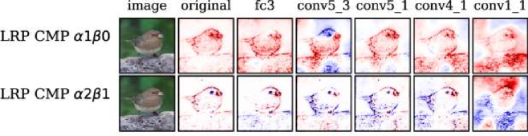
LRP_CMP

(Kohlbrenner et al., 2019; Lapuschkin et al., 2017) use LRP_z for the final dense layers and LRP_αβ for the convolutional layer. We report results for $\alpha=1,2$ as in (Kohlbrenner et al., 2019) in Figure 6(a).

For VGG-16, the saliency maps change when the network parameters are randomized. However, structurally, the underlying image structure seems to be scaled only locally (see Figure 6(a)). Inspecting the CSC path of the two LRP_CMP variants in Figure 6(c), we can see why. For dense layers, both methods do not converge as LRP_z is used, but the convergence start when LRP_αβ is applied. The relevance vectors of the dense layer can change the coarse local scaling. However, they cannot alter the direction of the relevance vectors of earlier layers to highlight different details.

In the backward-pass of the ResNet-50, the global-averaging layer assigns the identical gradient vector to each location of the last convolutional layer. Furthermore, the later convolutional layers operate on (7x7), where even a few 3x3 convolutions have a dense field-of-view. LRP_CMP does not resolve the global convergence for the ResNet-50.

Contrastive LRP

(Gu et al., 2018) noted the lack of class sensitivity and proposed to increase it by subtracting two saliency maps. The first saliency map explains only the logit ${\bm{y}}_{k}={\bm{y}}\odot{\bm{m}}_{k}$, where ${\bm{m}}_{k}$ is a one-hot vector and the second explains the opposite ${\bm{y}}_{\neg k}={\bm{y}}\odot(1-{\bm{m}}_{k})$:

$$\begin{split}\max(0,&n(r_{{\bm{x}}}^{z^{+}}({\bm{x}}|r_{\text{logits}}{:\leavevmode\resizebox{3.33333pt}{0.0pt}{=}}{\bm{y}}_{k}))\\ &-n(r_{{\bm{x}}}^{z^{+}}({\bm{x}}|r_{\text{logits}}{:\!\leavevmode\resizebox{3.33333pt}{0.0pt}{=}}\,{\bm{y}}_{\neg k}))\end{split}$$ (15)

$n(.)$ normalizes each saliency map by its sum. The results of Contrastive LRP are similar to Figre 1(e), no $\max$ is applied. The underlying convergence problem is not resolved.

Contrastive Excitation BP

The lack of class sensitivity of the $z^{+}$-rule was noted in (Zhang et al., 2018) and to increase it, they proposed to change the backpropagation rule of the final fully-connected layer to:

$$r^{\text{cEBP}}_{\text{final fc}}(x)=(Z^{+}_{\text{final fc}}-N^{+}_{\text{final fc}}){\bm{m}}_{k},$$ (16)

where ${\bm{m}}_{k}$ is a one-hot vector selecting the explained class. The added $N^{+}_{\text{final fc}}$ is computed as the $Z^{+}_{\text{final fc}}$ but on the negative weights $-W_{\text{final fc}}$. Note that the combination of the two matrices introduces negative entries. Class sensitivity is increased. It does also not resolve the underlying convergence problem. If, for example, more fully-connected layers would be used, the saliency maps would become globally class insensitive again.

Texture vs. Contours

(Geirhos et al., 2019) found that deep convolutional networks are more sensitive towards texture and not the shape of the object. For example, the shape of a cat filled with an elephant texture will be wrongly classified as an elephant. However, modified BP methods highlight the contours of objects rather.

Recurrent Neural Networks

Modified BP methods are focused on convolutional neural networks and are mostly applied on vision tasks. The innvestigate package does not yet support recurrent models. To our knowledge, (Arras et al., 2017) is the only work that applied modified BP rules to RNNs (LRP_z for LSTMs). Training, and applying modified backpropagation rules to RNNs, involves unrolling the network, essentially transforming it to a feed-forward architecture. Due to our theoretical results, modified BP rules that yield positive relevance matrices (e.g. $z^{+}$-rule) will converge. However, further work would be needed to measure how RNN architectures (LSTM, GRU) differ in their specific convergence behavior.

Not Converging Attribution Methods

Besides modified BP attribution methods, there also exist gradient averaging and black-box methods. SmoothGrad (Smilkov et al., 2017) and Integrated Gradients (Sundararajan et al., 2017) average the gradient. CAM and Grad-CAM (Zhou et al., 2016; Selvaraju et al., 2017) determine important areas by the activation of the last convolutional layer. Black-box attribution methods only modify the model’s input but do not rely on the gradient or other model internals. The most prominent black-box methods are Occlusion, LIME, SHAP (Zeiler & Fergus, 2014; Ribeiro et al., 2016; Lundberg & Lee, 2017). IBA (Schulz et al., 2020) applies an information bottleneck to remove unimportant information. TCAV (Kim et al., 2018) explains models using higher-level concepts.

All here mentioned attribution methods do not converge, as they either rely on the gradient or treat the model as black-box. Only when the BP algorithm is modified, the convergence problem can occur. The here mentioned algorithms might still suffer from other limitations.

Limitations

Also, we tried to include most modified BP attribution methods, we left some out for our evaluation (Nam et al., 2019; Wang et al., 2019; Huber et al., 2019). In our theoretical analysis of PatternAttribution, we based our argument on why it converges on empirical observations performed on a single set of pattern matrices.

6 Related Work

Limitations of attribution

The limitations of explanation methods were studied before. (Viering et al., 2019) alter the explanations of Grad-CAM arbitrarily by modifying the model architecture only slightly. Similarly, (Slack et al., 2020) construct a biased classifier that can hide its biases from LIME and SHAP. The theoretic analysis (Nie et al., 2018) indicates that GuidedBP tends to reconstruct the input instead of explaining the network’s decision. (Adebayo et al., 2018) showed GuidedBP to be independent of later layers’ parameters. (Atrey et al., 2020) tested saliency methods in a reinforcement learning setting.

(Kindermans et al., 2018) show that LRP, GuidedBP, and Deconv produce incorrect explanations for linear models if the input contains noise. (Rieger, 2017; Zhang et al., 2018; Gu et al., 2018; Kohlbrenner et al., 2019; Montavon et al., 2019; Tsunakawa et al., 2019) noted the class-insensitivity of different modified BP methods, but they rather proposed ways to improve the class sensitivity than to provide correct reasons why modified BP methods are class insensitive. Other than argued in (Gu et al., 2018), the class insensitivity is not caused by missing ReLU masks and Pooling switches. To the best of our knowledge, we are the first to identify the reason why many modified BP methods do not explain the decision of deep neural networks faithfully.

Evaluation metrics for attribution

As no ground-truth data exists for feature importance, different proxy tasks were proposed to measure the performance of attribution algorithms. One approach is to test how much relevance falls into ground-truth bounding boxes (Schulz et al., 2020; Zhang et al., 2018).

The MoRF and LeRF evaluation removes the most and least relevant input features and measures the change in model performance (Samek et al., 2016). The relevant image parts are masked usually to zero. On these modified samples, the model might not be reliable. The ROAR score improves it by retraining the model from scratch (Hooker et al., 2018). While computationally expensive, it ensures the model performance does not drop due to out-of-distribution samples. The ROAR performance of Int.Grad. and GuidedBP is equally bad, worse than a random baseline (see Figre 4 in (Hooker et al., 2018)). Thus, ROAR does not separate converging from non-converging methods.

Our CSC measure has some similarities with the work (Balduzzi et al., 2017), which analyzes the effect of skip connections on the gradient. They measure the convergence between the gradient vector from different samples using the effective rank (Vershynin, 2012). The CSC metric applies to modified BP methods and is an efficient tool to trace the degree of convergence.

A different approach to verify attribution methods is to measure how helpful they are for humans (Alqaraawi et al., 2020; Doshi-Velez & Kim, 2017; Lage et al., 2018).

7 Conclusion

In our paper, we analyzed modified BP methods, which aim to explain the predictions of deep neural networks. Our analysis revealed that most of these attribution methods have theoretical properties contrary to their goal. PatternAttribution and LRP cite Deep Taylor Decomposition as the theoretical motivation. In the light of our results, revisiting the theoretical derivation of Deep Taylor Decomposition may prove insightful. Our theoretical analysis stresses the importance of negative relevance values. A possible way to increase class-sensitivity and resolve the convergence problem could be to backpropagate negative relevance similar to DeepLIFT, the only method passing our test.

8 Acknowledgements

We are grateful to the comments by our reviewers, which help to improve the manuscript further. We thank Benjamin Wild and David Dormagen for stimulating discussions. We also thank Avanti Shrikumar for answering our questions and helping us with the DeepLIFT implementation. The comments by Agathe Balayn, Karl Schulz, and Julian Stastny improved the manuscript. A special thanks goes to the anonymous reviewer 1 of our paper (Schulz et al., 2020), who encouraged us to report results on the sanity checks — the starting point of this paper. The Elsa-Neumann-Scholarship by the state of Berlin supported LS. We are also grateful to Nvidia for a Titan Xp and to ZEDAT for access their HPC system.

Appendix A Proof of Theorem 1

In (Friedland, 2006) the theorem is proven for square matrices. In fact Theorem 1 can be deduced from this case by the following argument:

For a sequence of non-square matrices $(A_{k})_{k\in\mathbb{N}}\in\mathbb{R}^{m_{k}\times l_{k}}$ of finite size $m_{k},l_{k}\leq L$ we can always find a finite set of subsequent matrices that when multiplied together are a square matrix.

$$\underbrace{A_{1}\cdot...\cdot A_{n_{1}}}_{=:\bar{A}_{1}\in\mathbb{R}^{m\times m}}\cdot\underbrace{A_{n_{1}+1}\cdot...\cdot A_{n_{2}}}_{=:\bar{A}_{2}\in\mathbb{R}^{m\times m}}\cdot\underbrace{A_{n_{2}+1}\cdot...\cdot A_{n_{3}}}_{=:\bar{A}_{3}\in\mathbb{R}^{m\times m}}\cdot...$$ (17)

The matrices $\bar{A}_{1},\bar{A}_{2},\bar{A}_{3},...$ define a sequence of non-negative square matrices that fulfill the conditions in (Friedland, 2006) and therefore converge to a rank-1 matrix.

Our proof requires no knowledge of algebraic geometry and uses the cosine similarity to show convergence. First, we outline the conditions on the matrix sequence $A_{n}$. Then, we state the theorem again and sketch our proof to give the reader a better overview. Finally, we prove the theorem in 5 steps.

Conditions on $A_{n}$

The first obvious condition is that the $(A_{n})_{n\in\mathbb{N}}$ is a sequence of non-negative matrices such that $A_{i}$, $A_{i+1}$ have the correct size to be multiplied together. Secondly, as we calculate angles between column vector in our proof, no column of $A_{n}$ should be zero. The angle between a zero vector and any other vector is undefined. Finally, the size of $A_{n}$ should not increase infinitely, i.e. an upper bound on the size of the $A_{i}$’s exists such that $A_{i}\in\mathbb{R}^{m\times l}$ where $m,l\leq L$ for some $L\in\mathbb{N}$.

Definition 1.

We say $\lim_{n\to\infty}A_{n}$ exists, if for all $m,l\in\mathbb{N}$ the subsequences $A_{n_{k(m,l)}}\in\mathbb{R}^{m\times l}$ that consist of all terms that have size $m\times l$ converge elementwise. Note that even if there only finitely many, say $A_{N}$ is the last term with $A_{n}\in\mathbb{R}^{m\times l}$, we say $\lim_{k\to\infty}A_{n_{k(l,m)}}=A_{N}$.

Theorem 1. Let $A_{1},A_{2},A_{3}\dots$ be a sequence of non-negative matrices as described above such that $\lim_{n\to\infty}A_{n}$ exists. We exclude the cases where one column of $\lim_{n\to\infty}A_{n}$ is the zero vector or two columns are orthogonal to each other. Then the product of all terms of the sequence converges to a rank-1 matrix $\bar{C}$:

$$\bar{C}:=\prod_{i=1}^{\infty}A_{i}=\bar{\bm{c}}\bm{\gamma}^{T}\,.$$ (18)

Matrices of this form are excluded for $\lim_{n\to\infty}A_{n}$:

$\begin{pmatrix}\makebox[0.0pt][l]{$\smash{\underbrace{\phantom{\begin{matrix}\begin{matrix}&&\\ {\bm{v}}_{1}&...&{\bm{v}}_{l}\\ &&\end{matrix}\end{matrix}}}_{\text{$\text{arbitrary}$}}}$}\begin{matrix}&&\\ {\bm{v}}_{1}&...&{\bm{v}}_{l}\\ &&\end{matrix}&\makebox[0.0pt][l]{$\smash{\underbrace{\phantom{\begin{matrix}\begin{matrix}&&\\ {\bm{v}}_{l+1}&...&{\bm{v}}_{m}\\ &&\end{matrix}\end{matrix}}}_{\text{$\text{orthogonal}$}}}$}\begin{matrix}&&\\ {\bm{v}}_{l+1}&...&{\bm{v}}_{m}\\ &&\end{matrix}&\makebox[0.0pt][l]{$\smash{\underbrace{\phantom{\begin{matrix}\begin{matrix}&&\\ {\bm{v}}_{m+1}&...&{\bm{v}}_{n}\\ &&\end{matrix}\end{matrix}}}_{\text{${\bm{v}}_{i}=0$}}}$}\begin{matrix}&&\\ {\bm{v}}_{m+1}&...&{\bm{v}}_{n}\\ &&\end{matrix}\end{pmatrix}$

$\begin{pmatrix}\begin{matrix}0&1\\ 1&1\\ 1&1\\ 1&1\end{matrix}&\begin{matrix}1&0\\ 0&0\\ 1&0\\ 0&1\end{matrix}&\begin{matrix}0&0\\ 0&0\\ 0&0\\ 0&0\end{matrix}\end{pmatrix}$

Theory

Example

up to ordering of the columns.

Proof sketch

To show that $\prod_{i}^{\infty}A_{i}$ converges to a rank-1 matrix, we do the following steps:

1. We define a sequence $s_{n}$ as the cosine of the maximum angle between the column vectors of $M_{n}:=\prod^{n}_{i=1}A_{i}$.

2. We show that the sequence $s_{n}$ is monotonic and bounded and therefore converging.

3. We assume $\lim_{n\to\infty}s_{n}\neq 1$ and analyze two cases where we do not get a contradiction. Each case yields an equation on $\lim_{n\to\infty}A_{n}$.

4. In both cases, we find lower bounds on $s_{n}$: $\alpha_{n}s_{n-1}$ and $\alpha^{\prime}_{n}s_{n-1}$ that are becoming infinitely large, unless we have $\lim_{n\to\infty}\alpha_{n}=1$ (case 1) or $\lim_{n\to\infty}\alpha^{\prime}_{n}=1$ (case 2).

5. The lower bounds lead to equations on $\lim_{n\to\infty}A_{n}$ for non-convergence. The only solutions, we obtain for $\lim_{n\to\infty}A_{n}$, are those explicitly excluded in the theorem. We still get a contradiction and $\lim_{n\to\infty}s_{n}=1\Rightarrow\prod_{i}^{\infty}A_{i}=\bar{c}\gamma^{T}$.

Proof    (1) Let $M_{n}:=\prod_{i=1}^{n}A_{i}$ be the product of the matrices $A_{1}\cdot\ldots\cdot A_{n}$. We define a sequence on the angles of column vectors of $M_{n}$ using the cosine similarity. Let ${\bm{v}}_{1}(n),...,{\bm{v}}_{k(n)}(n)$ be the column vectors of $M_{n}$. Note, the angles are well defined between the columns of $M_{n}$. The columns of $M_{n}$ cannot be a zero vector as we required $A_{n}$ to have no zero columns. Let $s_{n}$ be the cosine of the maximal angle between the columns of $M_{n}$:

$$s_{n}=\operatorname{min}_{i\neq j}\operatorname{s_{\cos}}({\bm{v}}_{i}(n),{\bm{v}}_{j}(n)):=\min_{i,j}\frac{\langle{\bm{v}}_{i}(n),{\bm{v}}_{j}(n)\rangle}{\|{\bm{v}}_{i}(n)\|\|{\bm{v}}_{j}(n)\|},$$ (19)

where $\langle\cdot,\cdot\rangle$ denotes the dot product. We show that the maximal angle converges to 0 as $\lim_{n\to\infty}s_{n}=1$, which is equivalent to $M_{n}$ converging to a rank-1 matrix. In the following, we take a look at two consecutive elements of the sequence $s_{n}$ and check by how much the sequence increases.

(2) We show that the sequence $s_{n}$ is monotonic and bounded and therefore converging. Assume ${\bm{a}}_{n+1}$ and ${\bm{b}}_{n+1}$ are the two columns of $A_{n+1}$ which produce the columns ${\bm{v}}_{m}(n+1)$ and ${\bm{v}}_{m^{\prime}}(n+1)$ of $M_{n+1}$ with the maximum angle:

$$s_{n+1}=\operatorname{s_{\cos}}({\bm{v}}_{m}(n+1),{\bm{v}}_{m^{\prime}}(n+1))=\operatorname{s_{\cos}}(M_{n}{\bm{a}}_{n+1},M_{n}{\bm{b}}_{n+1}).$$ (20)

We also assume that $\|{\bm{v}}_{i}(n)\|=1$ for all $i$, since the angle is independent of length. To declutter notation, we write ${\bm{v}}_{i}(n)=:{\bm{v}}_{i}$, ${\bm{a}}_{n}={\bm{a}}=(a_{1},...,a_{k})^{T}$ and ${\bm{b}}_{n}={\bm{b}}=(b_{1},...,b_{k})^{T}$. We now show that $s_{n}$ is monotonic and use the definition of the cosine similarity:

$$s_{n+1}=\frac{\sum_{ij}a_{i}b_{j}\langle{\bm{v}}_{i},{\bm{v}}_{j}\rangle}{\|\sum_{i}a_{i}{\bm{v}}_{i}\|\|\sum_{i}b_{i}{\bm{v}}_{i}\|}$$ (21)

Using the triangle inequality $\|\sum_{i}a_{i}{\bm{v}}_{i}\|\leq\sum_{i}a_{i}\|{\bm{v}}_{i}\|$ we get:

$$s_{n+1}\geq\frac{\sum_{ij}a_{i}b_{j}\langle{\bm{v}}_{i},{\bm{v}}_{j}\rangle}{(\sum_{i}a_{i}\|{\bm{v}}_{i}\|)(\sum_{i}b_{i}\|{\bm{v}}_{i}\|)}$$ (22)

As we assumed that the $\left\lVert{\bm{v}}_{i}\right\rVert=1$, we know that $\langle{\bm{v}}_{i},{\bm{v}}_{j}\rangle=s_{\cos}({\bm{v}}_{i},{\bm{v}}_{j})$ which must be greater than the smallest cosine similarity $s_{n}$:

$$s_{n+1}\geq\frac{\sum_{ij}a_{i}b_{j}\langle{\bm{v}}_{i},{\bm{v}}_{j}\rangle}{(\sum_{i}a_{i})(\sum_{i}b_{i})}\geq\frac{\sum_{ij}a_{i}b_{j}}{(\sum_{i}a_{i})(\sum_{i}b_{i})}s_{n}=s_{n}$$ (23)

Therefore $s_{n}$ is monotonically increasing and upper-bounded by $1$ as the cosine. Due to the monotone convergence theorem, it will converge. The rest of the proof investigates if the sequence $s_{n}$ converges to 1 and if so, under which conditions.

(3) We look at two consecutive sequence elements and measure the factor $\alpha$ by which they increase: $s_{n+1}\geq\alpha s_{n}$. We are using proof by contradiction and assume that $s_{n}$ does not converge to 1. We get two cases, each with a lower bound on the factor of increase. For both cases, we find a lower bound for $\alpha>1$ for all $n$ which would mean that $s_{n}$ is diverging to $\infty$ – a contradiction. Under certain conditions on $\lim_{n\to\infty}A_{n}$, we do not find a lower bound $\alpha>1$. We find that these conditions correspond to the conditions explicitly excluded in the theorem and therefore $M_{n}$ converges to a rank-1 matrix.

Case 1: Let $t_{n}:=\langle{\bm{v}}_{l}(n),{\bm{v}}_{m}(n)\rangle$ ($l\neq m$) and assume that there exists a subsequence $t_{n_{k}}$ of $t_{n}$ that does not converge to $\lim_{n\to\infty}s_{n}$. So there is an $\varepsilon>0$ such that $\langle{\bm{v}}_{l}(n_{k}),{\bm{v}}_{m}(n_{k})\rangle\geq(1+\varepsilon)s_{n_{k}}$ for all $k\geq K$ for some $K\in\mathbb{N}$.

We multiply the first lower bound of equation 23 by $1=\frac{s_{n}}{s_{n}}$ and get:

$$s_{n+1}\geq\frac{\sum_{ij}a_{i}b_{j}\langle{\bm{v}}_{i},{\bm{v}}_{j}\rangle}{\left(\sum_{i}a_{i}\right)\left(\sum_{i}b_{i}\right)}=\frac{\sum_{ij}a_{i}b_{j}\frac{\langle{\bm{v}}_{i},{\bm{v}}_{j}\rangle}{s_{n}}}{\left(\sum_{i}a_{i}\right)\left(\sum_{i}b_{i}\right)}s_{n},$$ (24)

We will now pull terms corresponding to the pair $(l,m)$ out of the sum and for all terms in the sum, we lower bound $\frac{\langle{\bm{v}}_{i},{\bm{v}}_{j}\rangle}{s_{n}}\geq 1$ by one. Let the set $I:=\{(i,j)\mid(i,j)\neq(l,m),(m,l)\}$ index all other terms:

$$s_{n+1}\geq\frac{\sum_{I}a_{i}b_{j}+(a_{l}b_{m}+a_{m}b_{l})\frac{\langle{\bm{v}}_{l},{\bm{v}}_{m}\rangle}{s_{n}}}{\left(\sum_{i}a_{i}\right)\left(\sum_{i}b_{i}\right)}s_{n}$$ (25)

We know that $\langle{\bm{v}}_{l}(n_{k}),{\bm{v}}_{m}(n_{k})\rangle\geq(1+\varepsilon)s_{n_{k}}$:

$$s_{n_{k+1}}\geq s_{n_{k}+1}\geq\frac{\sum_{I}a_{i}b_{j}+(a_{l}b_{m}+a_{m}b_{l})(1+\varepsilon)}{\left(\sum_{i}a_{i}\right)\left(\sum_{i}b_{i}\right)}s_{n_{k}}$$ (26)

We absorb the $m$, $l$ factors back into the sum:

$$s_{n_{k+1}}\geq\frac{\sum_{ij}a_{i}b_{j}+\overbrace{(a_{l}b_{m}+a_{m}b_{l})}^{=:r_{n_{k}}}\varepsilon}{\left(\sum_{i}a_{i}\right)\left(\sum_{i}b_{i}\right)}s_{n_{k}}=\left(1+\frac{r_{n_{k}}\varepsilon}{\left(\sum_{i}a_{i}\right)\left(\sum_{i}b_{i}\right)}\right)s_{n_{k}}\geq\underbrace{\Big{(}1+\frac{r_{n_{k}}\varepsilon}{\bar{q}}\Big{)}}_{=:\alpha_{n_{k}}}s_{n_{k}}$$ (27)

where $\bar{q}$ is an upper bound on $\sum_{ij}a_{i}b_{j}$ which exists since $\lim_{n\to\infty}A_{n}$ exists, which is also why $\lim_{k\to\infty}r_{n_{k}}$ exists.

(4) Case 1: Define $r_{n}=a_{l}(n)b_{m}(n)+a_{m}(n)b_{l}(n)$ analogous to $r_{n_{k}}$. So if $\lim_{n\to\infty}r_{n}=\lim_{k\to\infty}r_{n_{k}}\neq 0$, the factor by which $s_{n}$ increases would be greater that one by a constant – a contradiction:

$$s_{n_{k}}\geq(1+c)^{n^{\prime}}s_{n_{1}}>0$$ (28)

where $n_{k}-n^{\prime}$ is the number of cases where $r_{n_{k}}=0$ and $c>0$ is a lower bound on the set $\{\frac{\varepsilon r_{n_{k}}}{\bar{q}}\neq 0\}$. As we assumed $\lim_{n\to\infty}r_{n}\neq 0$, $c>0$ for an infinite number of cases and therefore $n^{\prime}\to\infty$ when $k\to\infty$.

To end case 1, we have to ensure that the first sequence element is greater than zero: $s_{n_{1}}\geq s_{1}>0$. This is not the case if the first $N$ matrices have two orthogonal columns, $s_{1}\!=\!...\!=\!s_{N}\!=\!0$. We can then skip the first $N$ matrices and define $s_{1}$ on $A_{N+1}$ (set $A_{i}=A_{N+i}$). We know $N$ has to be finite, as $\lim_{n\to\infty}A_{n}$ has no two columns that are orthogonal.

(3) Case 2: No subsequence of $t_{n}$, as defined in case 1, exists , i.e. for all $\varepsilon>0$ no subsequence $t_{n_{k}}=\langle{\bm{v}}_{l}(n),{\bm{v}}_{m}(n)\rangle\geq(1+\varepsilon)s_{n_{k}}$ exists. Then $t_{n}$ and $s_{n}$ converge to the same value: $\lim_{n\to\infty}t_{n}-s_{n}=0$. Since we assumed that $s_{n}$ does not converge to one, it must converge to a value smaller than 1 by a constant $\varepsilon^{\prime}$. An $N\in\mathbb{N}$ exists such that for all $n\geq N$ there is an $\varepsilon^{\prime}>0$ with $\langle{\bm{v}}_{l}(n),{\bm{v}}_{m}(n)\rangle\leq 1-\varepsilon^{\prime}$. We derive a second lower bound:

$$s_{n+1}=\frac{\sum_{ij}a_{i}b_{j}\langle{\bm{v}}_{i},{\bm{v}}_{j}\rangle}{\|\sum_{i}a_{i}{\bm{v}}_{i}\|\|\sum_{i}b_{i}{\bm{v}}_{i}\|}\geq\frac{\sum_{ij}a_{i}b_{j}}{\|\sum_{i}a_{i}{\bm{v}}_{i}\|\|\sum_{i}b_{i}{\bm{v}}_{i}\|}s_{n},$$ (29)

where we used $\langle{\bm{v}}_{i},{\bm{v}}_{j}\rangle\geq s_{n}$. We now find a lower bound for the square of this factor. The steps are similar to case 1:

$$\frac{(\sum_{ij}a_{i}b_{j})^{2}}{\|\sum_{i}a_{i}{\bm{v}}_{i}\|^{2}\|\sum_{i}b_{i}{\bm{v}}_{i}\|^{2}} =\frac{(\sum_{ij}a_{i}b_{j})^{2}}{(\sum_{ij}a_{i}a_{j}\langle{\bm{v}}_{i},{\bm{v}}_{j}\rangle)(\sum_{ij}b_{i}b_{j}\langle{\bm{v}}_{i},{\bm{v}}_{j}\rangle)}$$ (30)

$$=\frac{(\sum_{ij}a_{i}b_{j})^{2}}{(\sum_{I}a_{i}a_{j}+2a_{l}a_{m}\langle{\bm{v}}_{l},{\bm{v}}_{m}\rangle)(\sum_{I}b_{i}b_{j}+2b_{l}b_{m}\langle{\bm{v}}_{l},{\bm{v}}_{m}\rangle)}$$ (31)

$$\geq\frac{(\sum_{ij}a_{i}b_{j})^{2}}{(\sum_{I}a_{i}a_{j}+2a_{l}a_{m}(1-\varepsilon^{\prime}))(\sum_{I}b_{i}b_{j}+2b_{l}b_{m}(1-\varepsilon^{\prime}))}$$ (32)

$$=\frac{q^{2}}{q^{2}-\varepsilon^{\prime}\left(\sum_{ij}2a_{l}a_{m}b_{i}b_{j}+\sum_{ij}2b_{l}b_{m}a_{i}a_{j}-4\varepsilon^{\prime}a_{l}a_{m}b_{l}b_{m}\right)}$$ (33)

$$\geq\frac{q^{2}}{q^{2}-\varepsilon^{\prime 2}\underbrace{\Big{(}\sum_{ij}2a_{l}a_{m}b_{i}b_{j}+\sum_{ij}2b_{l}b_{m}a_{i}a_{j}-4a_{l}a_{m}b_{l}b_{m}\Big{)}}_{=:r_{n}^{\prime}}}$$ (34)

$$=\frac{q^{2}}{q^{2}-\varepsilon^{\prime 2}r_{n}^{\prime}}=1+\frac{\varepsilon^{\prime 2}r_{n}^{\prime}}{q^{2}-\varepsilon^{\prime 2}r_{n}^{\prime}}\geq 1+\frac{\varepsilon^{\prime 2}r_{n}^{\prime}}{\bar{q}^{2}-\varepsilon^{\prime 2}r_{n}^{\prime}}=:\alpha^{\prime 2}_{n}$$ (35)

where $q^{2}=(\sum_{ij}a_{i}b_{j})^{2}$ and $\bar{q}^{2}$ is an upper bound on $q^{2}$ for all $n$. Note that $q^{2}-\varepsilon^{\prime 2}r_{n}^{\prime}>0$, since $q^{2}$ has all terms that $r_{n}^{\prime}$ has but more.

(4) Case 2: So $r_{n}^{\prime}$ is a sequence that converges to zero. Otherwise, the factor by which $s_{n}$ increases would be greater than one by at least a constant for infinitely many $n$. As in the previous case 1, this would lead to a contradiction.

(5) Case 1 and case 2 are complements from which we obtain two equations for $\lim_{n\to\infty}A_{n}$. Let ${\bm{a}}_{k}=(a_{1},...,a_{k})^{T}$ and ${\bm{b}}_{k}=(b_{1},...,b_{k})^{T}$ be columns of $\lim_{n\to\infty}A_{n}$. We get one equation per case. For all $(i,j)$ with $i<j$ we have:

$$\text{{Case 1:}}\lim_{n\to\infty}r_{n}=0\Rightarrow a_{i}b_{j}=a_{j}b_{i}=0\quad\text{ or }\quad\text{{Case 2:}}\lim_{n\to\infty}r^{\prime}_{n}=0\Rightarrow a_{i}a_{j}=b_{i}b_{j}=0,$$ (36)

where the first equation comes from $\lim_{n\to\infty}r_{n}=0$ and the second from $\lim_{n\to\infty}r_{n}^{\prime}=0$.

For equation 36 to be true, the following set of equations have to hold:

$$S(k):=\{\forall i=1,...,k:a_{i}=0\neq b_{i},a_{i}\neq 0=b_{i}\text{ or }a_{i}=b_{i}=0\}$$ (37)

$$\cup\quad\{\exists l:a_{l}\neq 0\neq b_{l}\text{ and }\forall i\neq l:a_{i}=b_{i}=0\}.$$ (38)

This is equivalent to the matrix being rank one already or one of the columns is the zero vector or two are orthogonal to each other. To show why this statement holds, we are using induction on $k$. For $k=2$, we have the following set of solutions:

$\begin{pmatrix}0&b_{1}\\ 0&b_{2}\end{pmatrix}\quad\begin{pmatrix}a_{1}&0\\ a_{2}&0\end{pmatrix}\quad\begin{pmatrix}0&0\\ a_{2}&b_{2}\end{pmatrix}\quad\begin{pmatrix}a_{1}&b_{1}\\ 0&0\end{pmatrix}$	$\begin{pmatrix}a_{1}&0\\ 0&b_{2}\end{pmatrix}\quad\begin{pmatrix}0&b_{1}\\ a_{2}&0\end{pmatrix}\quad$
Case 1	Case 2

Case one provides rank 1 matrices only and case two gives orthogonal columns. So, the statement holds for $k=2$.

Next assume we solved the problem for columns with $k$ entries and want to deduce the case where we have $k+1$ entries (i.e. they satisfy the equations in $S(k+1)$). The pair $a_{k+1},b_{k+1}$ satisfies either one of the three equations in line equation 37: $a_{k+1}=b_{k+1}=0$, $a_{k+1}=0\neq b_{k+1}$ or $a_{k+1}\neq 0=b_{k+1}$. If $a_{k+1}=b_{k+1}=0$, the rest of the non-trivial equations will be the same set of equations that one will get in the case of $k$ entries. If $a_{k+1}=0\neq b_{k+1}$, we would be left with equation $a_{i}b_{k+1}=0$ (Case 1) or $b_{i}b_{k+1}=0$ (Case 2) which would mean that for all $i\leq k$ either $a_{i}=0$ or $b_{i}=0$, which will satisfy the equations in $S(k+1)$. We get an analogous argument in the case of $a_{k+1}\neq 0=b_{k+1}$.

The other possibility is that $a_{k+1}\neq 0\neq b_{k+1}$. But in this case both equations from case one and two $a_{k+1}b_{i}=a_{i}b_{k+1}=0$ and $a_{k+1}a_{i}=b_{k+1}b_{i}=0$ lead to $a_{i}=b_{i}=0$ for all $i\leq k$ and this satisfies $S(k+1)$ in line equation 38, concluding the induction.

This completes the proof. Since $\lim_{n\to\infty}s_{n}\neq 1$ only if $\lim_{n\to\infty}A_{n}$ has a column that is the zero vector, a multiple of a standard basis vector or it has two columns that are orthogonal to each. Exactly, the conditions excluded in the theorem. For all other cases, we get a contradiction: therefore $\lim_{n\to\infty}s_{n}=1$ and $M_{n}$ converges to a rank-1 matrix. ∎

Appendix B Convergence Speed & Simulation of Matrix Convergences

(a) different matrix properties (see text)

(b) $\alpha W^{+}+\beta W^{-}$ where $W_{[ij]}\sim\mathcal{N}(0,1)$

Figure 7: Simulated convergence for a matrix chain.

We proved that $M_{n}=\prod_{i}^{n}A_{i}$ converges to a rank-1 matrix for $n\to\infty$, but which practical implications has this for a 16 weight-layered network? How quickly is the convergence for matrices considered in neural networks?

We know that $s_{n}$ increases by a factor $(1+c)$ greater than 1 ($c>0$):

$$s_{n}\geq(1+c)s_{n-1}$$ (39)

Each iteration yields such a factor and we get a chain of factors:

$$s_{n}\geq(1+c_{n})(1+c_{n-1})...(1+c_{2})s_{1}$$ (40)

Although the multiplication chain of $c_{n}$ has some similarities to an exponential form $\gamma^{n}$, $s_{n}$ does not have to converge exponentially as the individual $c_{n}$ have to decrease ($s_{n}$ bounded by $1$). We investigated the convergence speed using a simulation of random matrices and find that non-negative matrices decay exponentially fast towards 1.

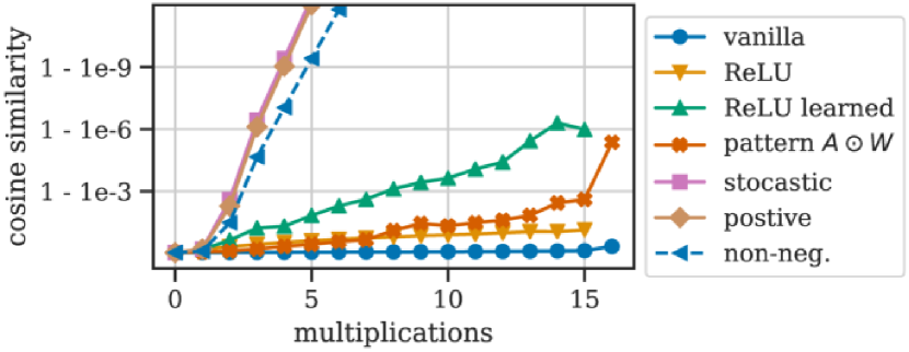
We report the converging behavior for matrix chains which resembles a VGG-16. As in the backward pass, we start from the last layer. The convolutional kernels are considered to be 1x1, e.g. for a kernel of size (3, 3, 256, 128), we use a matrix of size (256, 128).

We test out the effect of different matrix properties. For vanilla, we sample the matrix entries from a normal distribution. Next, we apply a ReLU operation after each multiplication. For ReLU learned, we used the corresponding learned VGG parameters. We generate non-negative matrices containing   50% zeros by clipping random matrices to $[0,\infty]$. And positive matrices by taking the absolute value. We report the median cosine similarity between the column vectors of the matrix.

The y-axis of Figure 7(a) has a logarithmic scale. We observe that the positive, stochastic, and non-negative matrices yield a linear path, indicating an exponential decay of the form: $1-\exp(-\lambda n)$. The 50% zeros in the non-negative matrices only result in a bit lower convergence slope. After 7 iterations, they converged to a single vector up to floating point imprecision.

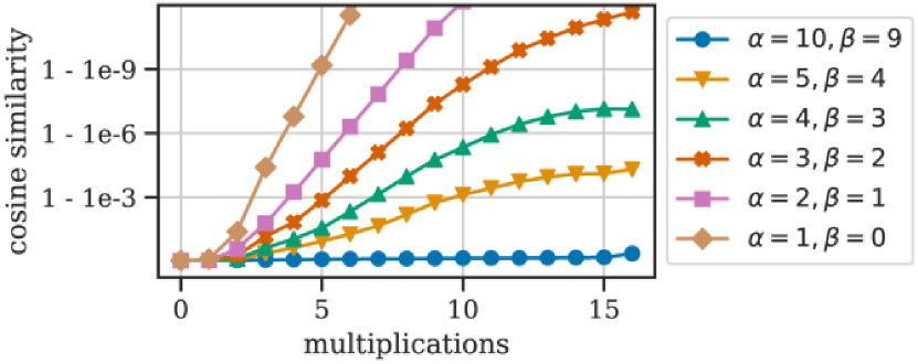
We also investigated how a slightly negative matrix influences the convergence. In Figure 7(b), we show the converges of matrices: $\alpha W^{+}+\beta W^{-}$ where $W^{+}=\max(0,W),W^{-}=\min(0,W)$ and $W\sim\mathcal{N}(0,I)$. We find that for small enough $\beta<4$ values the matrix chains still converge. This simulation motivated us to include LRP_α5β4 in our evaluation which show less convergence on VGG-16, but its saliency maps also contain more noise.

Appendix C Pattern Attribution

We derive equation 9 from the original equation given in (Kindermans et al., 2018). We will use the notation from the original paper and denote a weight vector with ${\bm{w}}=W_{l_{[i,:]}}$ and the corresponding pattern with ${\bm{a}}=A_{l_{[i,:]}}$. The output is $y={\bm{w}}^{T}{\bm{x}}$.

Derivation of Pattern Computation

For the positive patterns of the two-component estimator $S_{{\bm{a}}+-}$, the expectation is taken only over $\{{\bm{x}}|{\bm{w}}^{T}{\bm{x}}>0\}$. We only show it for the positive patterns ${\bm{a}}_{+}$. As our derivation is independent of the subset of ${\bm{x}}$ considered, it would work analogously for negative patterns or the linear estimator $S_{\bm{a}}$.

The formula to compute the pattern ${\bm{a}}_{+}$ is given by:

$$\begin{split}{\bm{a}}_{+}&=\frac{\mathbb{E}_{+}\left[{\bm{x}}y\right]-\mathbb{E}_{+}\left[{\bm{x}}\right]\mathbb{E}_{+}\left[y\right]}{{\bm{w}}^{T}\mathbb{E}_{+}\left[{\bm{x}}y\right]-{\bm{w}}^{T}\mathbb{E}_{+}\left[{\bm{x}}\right]\mathbb{E}_{+}\left[y\right]}\\ &=\frac{\operatorname{cov}[{\bm{x}},{\bm{w}}^{T}{\bm{x}}]}{{\bm{w}}^{T}\operatorname{cov}[{\bm{x}},{\bm{w}}^{T}{\bm{x}}]},\end{split}$$ (41)

where $\operatorname{cov}[{\bm{x}},{\bm{w}}^{T}{\bm{x}}]=\mathbb{E}_{+}[{\bm{x}}y]-\mathbb{E}_{+}[{\bm{x}}]\mathbb{E}_{+}[y]$. Using the bilinearity of the covariance matrix ($\operatorname{cov}[{\bm{b}},{\bm{c}}^{T}{\bm{d}}]=\operatorname{cov}[{\bm{b}},{\bm{d}}]{\bm{c}}$), gives:

$${\bm{a}}_{+}=\frac{\operatorname{cov}[{\bm{x}},{\bm{x}}]{\bm{w}}}{{\bm{w}}^{T}\operatorname{cov}[{\bm{x}},{\bm{x}}]{\bm{w}}}.$$ (42)

Using the notation $\operatorname{cov}[{\bm{h}}]=\operatorname{cov}[{\bm{x}},{\bm{x}}]$ gives equation 9.

Connection to power iteration

A step of the power iteration is given by:

$${\bm{v}}_{k+1}=\frac{M{\bm{v}}_{k}}{\left\lVert M{\bm{v}}_{k}\right\rVert}$$ (43)

The denominator in equation 9 is ${\bm{w}}^{T}\operatorname{cov}[{\bm{h}}]{\bm{w}}$. Using the symmetry of $\operatorname{cov}[{\bm{h}}]$, we have:

$$\left\lVert\operatorname{cov}[{\bm{h}}]^{1/2}{\bm{w}}\right\rVert=({\bm{w}}^{T}\operatorname{cov}[{\bm{h}}]^{1/2}\operatorname{cov}[{\bm{h}}]^{1/2}{\bm{w}})^{1/2}=({\bm{w}}^{T}cov[{\bm{h}}]{\bm{w}})^{1/2}$$ (44)

This should be similar to the norm $\left\lVert\operatorname{cov}[h]{\bm{w}}\right\rVert$. As only a single step of the power iteration is performed, the scaling should not matter that much. The purpose of the scaling in the power-iteration algorithm is to keep the vector $v_{k}$ from exploding or converging to zero.

Appendix D CIFAR-10 Network Architecture

⬇

# network architecture as a keras model

model = Sequential()

model.add(InputLayer(input_shape=(32, 32, 3), name=’input’))

model.add(Conv2D(32, (3, 3), padding=’same’, name=’conv1’))

model.add(Activation(’relu’, name=’relu1’))

model.add(Conv2D(64, (3, 3), padding=’same’, name=’conv2’))

model.add(Activation(’relu’, name=’relu2’))

model.add(MaxPooling2D(pool_size=(2, 2), name=’pool2’))

model.add(Conv2D(128, (3, 3), padding=’same’, name=’conv3’))

model.add(Activation(’relu’, name=’relu3’))

model.add(Conv2D(128, (3, 3), padding=’same’, name=’conv4’))

model.add(Activation(’relu’, name=’relu4’))

model.add(MaxPooling2D(pool_size=(2, 2), name=’pool4’))

model.add(Flatten(name=’flatten’))

model.add(Dropout(0.5, name=’dropout5’))

model.add(Dense(1024, name=’fc5’))

model.add(Activation(’relu’, name=’relu5’))

model.add(Dropout(0.5, name=’dropout6’))

model.add(Dense(10, name=’fc6’))

model.add(Activation(’softmax’, name=’softmax’))

Appendix E Results on ResNet-50

(a) Random Logits

(b) Cascading Parameter Randomization

Figure 8: Effect of (a) randomizing the logits or (b) the parameters on a ResNet-50.

Appendix F Additional Cosine Similarity Figures

(a) ResNet-50 (linear)

(b) ResNet-50 (log)

(c) VGG-16

(d) ResNet-50

(e) VGG-16

(f) VGG-16

(g) VGG-16 (linear)

(h) CIFAR-10 (linear)

Figure 9: Convergence measured using the CSC for different starting layers.

Appendix G Saliency maps for Sanity Checks

For visualization, we normalized the saliency maps to be in $[0,1]$ if the method produce only positive relevance. If the method also estimates negative relevance, than it is normalized to $[-1,1]$. The negative and positive values are scaled equally by the absolute maximum. For the sanity checks, we scale all saliency maps to be in $[0,1]$.

(a) VGG-16.

(b) ResNet-50.

Figure 10: Saliency maps for sanity checks. Parameters are randomized starting from last to first layer.

References

- Adebayo et al. (2018) Adebayo, J., Gilmer, J., Muelly, M., Goodfellow, I., Hardt, M., and Kim, B. Sanity checks for saliency maps. In Advances in Neural Information Processing Systems, pp. 9505–9515, 2018.
- Alber et al. (2019) Alber, M., Lapuschkin, S., Seegerer, P., Hägele, M., Schütt, K. T., Montavon, G., Samek, W., Müller, K.-R., Dähne, S., and Kindermans, P.-J. innvestigate neural networks! Journal of Machine Learning Research, 20(93):1–8, 2019.
- Alqaraawi et al. (2020) Alqaraawi, A., Schuessler, M., Weiß, P., Costanza, E., and Berthouze, N. Evaluating saliency map explanations for convolutional neural networks: A user study. In Proceedings of the 25th International Conference on Intelligent User Interfaces, IUI ’20, pp. 263–274, New York, NY, USA, 2020. Association for Computing Machinery. doi: 10.1145/3377325.3377519.
- Ancona et al. (2017) Ancona, M., Ceolini, E., Öztireli, C., and Gross, M. A unified view of gradient-based attribution methods for deep neural networks. In NIPS 2017-Workshop on Interpreting, Explaining and Visualizing Deep Learning. ETH Zurich, 2017.
- Ando et al. (1987) Ando, T., Horn, R. A., and Johnson, C. R. The singular values of a hadamard product: a basic inequality. Linear and Multilinear Algebra, 21(4):345–365, 1987. doi: 10.1080/03081088708817810.
- Arras et al. (2017) Arras, L., Montavon, G., Müller, K.-R., and Samek, W. Explaining Recurrent Neural Network Predictions in Sentiment Analysis. In Proceedings of the EMNLP 2017 Workshop on Computational Approaches to Subjectivity, Sentiment and Social Media Analysis, pp. 159–168. Association for Computational Linguistics, 2017.
- Atrey et al. (2020) Atrey, A., Clary, K., and Jensen, D. Exploratory Not Explanatory: Counterfactual Analysis of Saliency Maps for Deep Reinforcement Learning. In International Conference on Learning Representations, April 2020.
- Bach et al. (2015) Bach, S., Binder, A., Montavon, G., Klauschen, F., Müller, K.-R., and Samek, W. On pixel-wise explanations for non-linear classifier decisions by layer-wise relevance propagation. PLoS ONE, 10(7), 2015. doi: 10.1371/journal.pone.0130140.
- Balduzzi et al. (2017) Balduzzi, D., Frean, M., Leary, L., Lewis, J., Ma, K. W.-D., and McWilliams, B. The shattered gradients problem: If resnets are the answer, then what is the question? In Proceedings of the 34th International Conference on Machine Learning-Volume 70, pp. 342–350. JMLR.org, 2017.
- Bergstra & Bengio (2012) Bergstra, J. and Bengio, Y. Random search for hyper-parameter optimization. Journal of Machine Learning Research, 13(Feb):281–305, 2012.
- Böhle et al. (2019) Böhle, M., Eitel, F., Weygandt, M., and Ritter, K. Layer-wise relevance propagation for explaining deep neural network decisions in mri-based alzheimer’s disease classification. Frontiers in Aging Neuroscience, 11:194, 2019. ISSN 1663-4365. doi: 10.3389/fnagi.2019.00194.
- Doshi-Velez & Kim (2017) Doshi-Velez, F. and Kim, B. Towards a rigorous science of interpretable machine learning. arXiv: 1702.08608, 2017.
- Efron (1979) Efron, B. Bootstrap methods: Another look at the jackknife. The Annals of Statistics, 7(1):1–26, 1979. ISSN 00905364.
- Eitel et al. (2019) Eitel, F., Soehler, E., Bellmann-Strobl, J., Brandt, A. U., Ruprecht, K., Giess, R. M., Kuchling, J., Asseyer, S., Weygandt, M., Haynes, J.-D., Scheel, M., Paul, F., and Ritter, K. Uncovering convolutional neural network decisions for diagnosing multiple sclerosis on conventional mri using layer-wise relevance propagation. NeuroImage: Clinical, 24, 2019. doi: https://doi.org/10.1016/j.nicl.2019.102003.
- Friedland (2006) Friedland, S. Convergence of products of matrices in projective spaces. Linear Algebra and its Applications, 413(2):247 – 263, 2006. ISSN 0024-3795. doi: https://doi.org/10.1016/j.laa.2004.06.021. Special Issue on the 11th Conference of the International Linear Algebra Society, Coimbra, 2004.
- Geirhos et al. (2019) Geirhos, R., Rubisch, P., Michaelis, C., Bethge, M., Wichmann, F. A., and Brendel, W. Imagenet-trained CNNs are biased towards texture; increasing shape bias improves accuracy and robustness. In International Conference on Learning Representations, 2019.
- Gu et al. (2018) Gu, J., Yang, Y., and Tresp, V. Understanding individual decisions of cnns via contrastive backpropagation. In Asian Conference on Computer Vision, pp. 119–134. Springer, 2018.
- Hajnal (1976) Hajnal, J. On products of non-negative matrices. Mathematical Proceedings of the Cambridge Philosophical Society, 79(3):521–530, May 1976. ISSN 0305-0041, 1469-8064.
- He et al. (2016) He, K., Zhang, X., Ren, S., and Sun, J. Deep residual learning for image recognition. In Proceedings of the IEEE conference on computer vision and pattern recognition, pp. 770–778, 2016.
- Hooker et al. (2018) Hooker, S., Erhan, D., Kindermans, P.-J., and Kim, B. Evaluating Feature Importance Estimates. arXiv: 1806.10758, 2018.
- Huber et al. (2019) Huber, T., Schiller, D., and André, E. Enhancing explainability of deep reinforcement learning through selective layer-wise relevance propagation. In KI 2019: Advances in Artificial Intelligence, pp. 188–202, Cham, 2019. Springer International Publishing. ISBN 978-3-030-30179-8.
- Kim et al. (2018) Kim, B., Wattenberg, M., Gilmer, J., Cai, C., Wexler, J., Viegas, F., et al. Interpretability beyond feature attribution: Quantitative testing with concept activation vectors (tcav). In International Conference on Machine Learning, pp. 2673–2682, 2018.
- Kim et al. (2019) Kim, B., Seo, J., Jeon, S., Koo, J., Choe, J., and Jeon, T. Why are Saliency Maps Noisy? Cause of and Solution to Noisy Saliency Maps. arXiv: 1902.04893, 2019.
- Kindermans et al. (2016) Kindermans, P.-J., Schütt, K., Müller, K.-R., and Dähne, S. Investigating the influence of noise and distractors on the interpretation of neural networks. arXiv: 1611.07270, 2016.
- Kindermans et al. (2018) Kindermans, P.-J., Schütt, K. T., Alber, M., Müller, K.-R., Erhan, D., Kim, B., and Dähne, S. Learning how to explain neural networks: Patternnet and patternattribution. In International Conference on Learning Representations, 2018.
- Kohlbrenner et al. (2019) Kohlbrenner, M., Bauer, A., Nakajima, S., Binder, A., Samek, W., and Lapuschkin, S. Towards best practice in explaining neural network decisions with lrp, 2019.
- Lage et al. (2018) Lage, I., Ross, A., Gershman, S. J., Kim, B., and Doshi-Velez, F. Human-in-the-loop interpretability prior. In Advances in Neural Information Processing Systems, pp. 10159–10168, 2018.
- Lapuschkin et al. (2017) Lapuschkin, S., Binder, A., Muller, K.-R., and Samek, W. Understanding and comparing deep neural networks for age and gender classification. In The IEEE International Conference on Computer Vision Workshops (ICCVW), Oct 2017.
- Lundberg & Lee (2017) Lundberg, S. M. and Lee, S.-I. A unified approach to interpreting model predictions. In Advances in Neural Information Processing Systems 30, pp. 4765–4774. Curran Associates, Inc., 2017.
- Montavon et al. (2017) Montavon, G., Lapuschkin, S., Binder, A., Samek, W., and Müller, K.-R. Explaining nonlinear classification decisions with deep taylor decomposition. Pattern Recognition, 65:211–222, 2017.
- Montavon et al. (2019) Montavon, G., Binder, A., Lapuschkin, S., Samek, W., and Müller, K.-R. Layer-wise relevance propagation: an overview. In Explainable AI: Interpreting, Explaining and Visualizing Deep Learning, pp. 193–209. Springer, 2019.
- Nam et al. (2019) Nam, W.-J., Gur, S., Choi, J., Wolf, L., and Lee, S.-W. Relative attributing propagation: Interpreting the comparative contributions of individual units in deep neural networks. arXiv:1904.00605, Nov 2019.
- Nie et al. (2018) Nie, W., Zhang, Y., and Patel, A. A theoretical explanation for perplexing behaviors of backpropagation-based visualizations. In International Conference on Machine Learning, pp. 3806–3815, 2018.
- Ribeiro et al. (2016) Ribeiro, M. T., Singh, S., and Guestrin, C. “why should i trust you?”: Explaining the predictions of any classifier. In Proceedings of the 22nd ACM SIGKDD International Conference on Knowledge Discovery and Data Mining, KDD ’16, pp. 1135–1144, New York, NY, USA, 2016. Association for Computing Machinery. ISBN 9781450342322. doi: 10.1145/2939672.2939778.
- Rieger (2017) Rieger, L. Separable explanations of neural network decisions. In NIPS 2017 Workshop on Interpretable Machine Learning, 2017.
- Russakovsky et al. (2015) Russakovsky, O., Deng, J., Su, H., Krause, J., Satheesh, S., Ma, S., Huang, Z., Karpathy, A., Khosla, A., Bernstein, M., Berg, A. C., and Fei-Fei, L. ImageNet Large Scale Visual Recognition Challenge. International Journal of Computer Vision (IJCV), 115(3):211–252, 2015. doi: 10.1007/s11263-015-0816-y.
- Samek et al. (2016) Samek, W., Binder, A., Montavon, G., Lapuschkin, S., and Müller, K.-R. Evaluating the visualization of what a deep neural network has learned. IEEE transactions on neural networks and learning systems, 28(11):2660–2673, 2016.
- Schiller et al. (2019) Schiller, D., Huber, T., Lingenfelser, F., Dietz, M., Seiderer, A., and André, E. Relevance-Based Feature Masking: Improving Neural Network Based Whale Classification Through Explainable Artificial Intelligence. In Proc. Interspeech 2019, pp. 2423–2427, 2019.
- Schulz et al. (2020) Schulz, K., Sixt, L., Tombari, F., and Landgraf, T. Restricting the flow: Information bottlenecks for attribution. In International Conference on Learning Representations, 2020.
- Selvaraju et al. (2017) Selvaraju, R. R., Cogswell, M., Das, A., Vedantam, R., Parikh, D., and Batra, D. Grad-cam: Visual explanations from deep networks via gradient-based localization. In Proceedings of the IEEE International Conference on Computer Vision, pp. 618–626, 2017.
- Shrikumar et al. (2016) Shrikumar, A., Greenside, P., Shcherbina, A., and Kundaje, A. Not just a black box: Learning important features through propagating activation differences. arXiv: 1605.01713, 2016.
- Shrikumar et al. (2017) Shrikumar, A., Greenside, P., and Kundaje, A. Learning important features through propagating activation differences. In Proceedings of the 34th International Conference on Machine Learning-Volume 70, pp. 3145–3153. JMLR.org, 2017.
- Simonyan & Zisserman (2014) Simonyan, K. and Zisserman, A. Very deep convolutional networks for large-scale image recognition. arXiv preprint arXiv:1409.1556, 2014.
- Slack et al. (2020) Slack, D., Hilgard, S., Jia, E., Singh, S., and Lakkaraju, H. Fooling lime and shap: Adversarial attacks on post hoc explanation methods. In Proceedings of the AAAI/ACM Conference on AI, Ethics, and Society, AIES ’20, pp. 180–186, New York, NY, USA, 2020. Association for Computing Machinery. doi: 10.1145/3375627.3375830.
- Smilkov et al. (2017) Smilkov, D., Thorat, N., Kim, B., Viégas, F., and Wattenberg, M. Smoothgrad: removing noise by adding noise. arXiv: 1706.03825, 2017.
- Springenberg et al. (2014) Springenberg, J. T., Dosovitskiy, A., Brox, T., and Riedmiller, M. Striving for Simplicity: The All Convolutional Net. arXiv: 1412.6806, 2014.
- Sturm et al. (2016) Sturm, I., Lapuschkin, S., Samek, W., and Müller, K.-R. Interpretable deep neural networks for single-trial eeg classification. Journal of neuroscience methods, 274:141–145, 2016.
- Sundararajan et al. (2017) Sundararajan, M., Taly, A., and Yan, Q. Axiomatic attribution for deep networks. In Proceedings of the 34th International Conference on Machine Learning-Volume 70, pp. 3319–3328. JMLR. org, 2017.
- Tsunakawa et al. (2019) Tsunakawa, H., Kameya, Y., Lee, H., Shinya, Y., and Mitsumoto, N. Contrastive relevance propagation for interpreting predictions by a single-shot object detector. In 2019 International Joint Conference on Neural Networks (IJCNN), pp. 1–9, July 2019. doi: 10.1109/IJCNN.2019.8851770.
- Vershynin (2012) Vershynin, R. Introduction to the non-asymptotic analysis of random matrices, pp. 210–268. Cambridge University Press, 2012. doi: 10.1017/CBO9780511794308.006.
- Viering et al. (2019) Viering, T., Wang, Z., Loog, M., and Eisemann, E. How to manipulate cnns to make them lie: the gradcam case, 2019.
- Wang et al. (2019) Wang, S., Zhou, T., and Bilmes, J. Bias also matters: Bias attribution for deep neural network explanation. In International Conference on Machine Learning, pp. 6659–6667, 2019.
- Wang et al. (2004) Wang, Z., Bovik, A. C., Sheikh, H. R., Simoncelli, E. P., et al. Image quality assessment: from error visibility to structural similarity. IEEE transactions on image processing, 13(4):600–612, 2004.
- Yang et al. (2018) Yang, Y., Tresp, V., Wunderle, M., and Fasching, P. A. Explaining therapy predictions with layer-wise relevance propagation in neural networks. In 2018 IEEE International Conference on Healthcare Informatics (ICHI), pp. 152–162, June 2018.
- Zeiler & Fergus (2014) Zeiler, M. D. and Fergus, R. Visualizing and understanding convolutional networks. In European conference on computer vision, pp. 818–833. Springer, 2014.
- Zhan (1997) Zhan, X. Inequalities for the Singular Values of Hadamard Products. SIAM Journal on Matrix Analysis and Applications, 18(4):1093–1095, October 1997. ISSN 0895-4798, 1095-7162. doi: 10.1137/S0895479896309645.
- Zhang et al. (2018) Zhang, J., Bargal, S. A., Lin, Z., Brandt, J., Shen, X., and Sclaroff, S. Top-down neural attention by excitation backprop. International Journal of Computer Vision, 126(10):1084–1102, 2018.
- Zhou et al. (2016) Zhou, B., Khosla, A., Lapedriza, A., Oliva, A., and Torralba, A. Learning deep features for discriminative localization. In 2016 IEEE Conference on Computer Vision and Pattern Recognition (CVPR), pp. 2921–2929, 2016.