Perturbation Monte Carlo Method for
Quantitative Photoacoustic Tomography

Abstract

Quantitative photoacoustic tomography aims at estimating optical parameters from photoacoustic images that are formed utilizing the photoacoustic effect caused by the absorption of an externally introduced light pulse. This optical parameter estimation is an ill-posed inverse problem, and thus it is sensitive to measurement and modeling errors. In this work, we propose a novel way to solve the inverse problem of quantitative photoacoustic tomography based on the perturbation Monte Carlo method. Monte Carlo method for light propagation is a stochastic approach for simulating photon trajectories in a medium with scattering particles. It is widely accepted as an accurate method to simulate light propagation in tissues. Furthermore, it is numerically robust and easy to implement. Perturbation Monte Carlo maintains this robustness and enables forming gradients for the solution of the inverse problem. We validate the method and apply it in the framework of Bayesian inverse problems. The simulations show that the perturbation Monte Carlo method can be used to estimate spatial distributions of both absorption and scattering parameters simultaneously. These estimates are qualitatively good and quantitatively accurate also in parameter scales that are realistic for biological tissues.

Photoacoustic tomography (PAT) is an imaging modality based on the photoacoustic effect generated by the absorption of an externally introduced light pulse in the imaged target. PAT combines optical contrast and specificity with the high spatial resolution of ultrasound. It has various applications in imaging of soft biological tissue, such as imaging human blood vessels, microvasculature of tumors and the cerebral cortex in small animals [1, 2, 3, 4, 5, 6, 7, 8]. Quantitative photoacoustic tomography (QPAT) continues from the conventional photoacoustic images and aims at estimating the spatial distributions of the optical parameters [9]. This optical inverse problem of QPAT is ill-posed, meaning that even small errors in measurements or modeling can lead to large errors in the solution. Therefore, solution of the QPAT inverse problem relies strongly on accurate modeling of light transport.

A widely accepted forward model for light propagation in scattering medium such as biological tissue is the radiative transfer equation (RTE) [10, 11]. Given the light source, geometry and the optical parameters of the medium, it can solve the light fluence and optical energy absorption into the tissue. Due to the computational complexity of the RTE, its approximations, such as the diffusion approximation, are generally applied in optical imaging [11]. However, the diffusion approximation is not valid in typical QPAT imaging situations where the size of the imaged targets corresponds approximately to a few scattering lengths. Alternatively to the deterministic models, the Monte Carlo method can be used to simulate light propagation in tissue. Monte Carlo is a stochastic method that can be used to simulate light tissue interactions. It has been widely utilized in biomedical optics, see e.g. [12, 13, 14, 15, 16], and various open-source Monte Carlo implementations have been published [13, 17, 18, 19, 20, 21].

The optical inverse problem of QPAT is typically formulated as a minimization problem that is solved using methods of numerical optimization [9]. Essentially, one minimizes the difference of the ’measured’ optical energy density and that produced by a numerical solution of a forward model. This is a large scale inverse problem with a large number of both unknown parameters and data points. Although methods for utilizing the RTE in the optical inverse problem have been presented [22, 23, 24, 25], the numerical implementations still suffer from the computationally expensive nature of the problem.

In this work, we use the Monte Carlo method in the solution of the optical inverse problem of QPAT. Previously Monte Carlo has been utilized in QPAT inverse problem by assuming the scattering as known and estimating the absorption [26, 27]. In practice, however, the scattering is not known and it needs to be taken into account when solving the inverse problem. Alternatively, adjoint Monte Carlo models of radiance have been applied to formulate the solution of the QPAT inverse problem [28, 29, 30]. This approach necessitates solving the radiance in several points in space and angular directions which causes challenges to storing the angular solution and having good enough sampling to allow an acceptable level of noise. The approach has been utilized in QPAT in estimating either absorption or scattering while keeping the other one as a known constant [28, 29], including a recent study with experimental data [30].

Herein, we introduce an approach to the QPAT inverse problem based on the so-called perturbation Monte Carlo (PMC) concept [31, 34]. In PMC, the aim is to evaluate the effect of a small change in the optical parameters, i.e. perturbation, efficiently. This is achieved by re-using the trajectories of photons from an unperturbed simulation so that the trajectories do not need to be re-generated for each perturbation [31]. Previously, PMC and a similar so-called white Monte Carlo approach have been utilized in other optical tomographic imaging modalities in diffuse optical tomography and fluorescence diffuse optical tomography for example in [32, 33, 34, 35, 36, 37, 38, 39, 40, 41]. Compared to the adjoint Monte Carlo, PMC does not require forming the radiance or its approximations, and thus it is numerically less expensive. We approach the QPAT inverse problem in the framework of the Bayesian inverse problems, and estimate both absorption and scattering simultaneously. A methodology for forming the Jacobian for the inverse problem of QPAT based on the PMC methodology is presented and validated. To our knowledge, this is the first work in which the PMC methodology is formulated for QPAT, and the first study in which the Monte Carlo method is used to estimate the spatial distributions of absorption and scattering parameters simultaneously in QPAT.

The rest of the paper is organized so that the forward model and the inverse problem of QPAT are described in Sec. 1. Monte Carlo is reviewed, PMC methodology is introduced, and formulation for Jacobians is provided in Sec. 2. The methodology is evaluated with simulations and discussed in Sec. 3 followed by conclusions in Sec. 4.

1 Forward and inverse problems of quantitative photoacoustic tomography

1.1 Forward model for quantitative photoacoustic tomography

Modeling photoacoustic effect consists of modeling optical light propagation and acoustic ultrasound propagation together with their coupling. Due to the difference in time-scales between the absorption of light and propagation of ultrasound, the pressure increase due to the absorption of light can be regarded as instantaneous with respect to the acoustic model. Therefore, in the optical model, a time-independent light transport model can be used. Further, the coupling of the optical and acoustic models can be described by a linear model.

1.1.1 Optical model

Let $r\in\mathbb{R}^{d}$ be a point located in a tissue region of interest $\Omega\subset\mathbb{R}^{d}$ with boundary $\partial\Omega$ where $d=2,3$ is the dimension of the domain, and and let $\hat{s}\in S^{d-1}$ denote a unit vector in the direction of interest. Light transport in biological tissue can be modeled with the radiative transfer equation

$$\begin{dcases}\hat{s}\cdot\nabla\phi(r,\hat{s})+(\mu_{\mathrm{s}}(r)+\mu_{\mathrm{a}}(r))\phi(r,\hat{s})\\ \qquad=\,\mu_{\mathrm{s}}(r)\int_{S^{d-1}}\Theta(\hat{s}\cdot\hat{s}^{\prime})\phi(r,\hat{s}^{\prime}){\rm d}\hat{s}^{\prime},\qquad r\in\Omega\\ \phi(r,{\hat{s}})=\left\{\begin{array}[]{cl}\phi_{0}(r,\hat{s}),&r\in\xi_{j},\quad\hat{s}\cdot{\hat{n}}<0\\ 0,&r\in\partial\Omega\backslash\xi_{j},\quad\hat{s}\cdot{\hat{n}}<0.\end{array}\right.\end{dcases}$$ (1)

where $\phi(r,\hat{s})$ is the radiance, $\mu_{\mathrm{s}}(r)$ is the scattering coefficient, $\mu_{\mathrm{a}}(r)$ is the absorption coefficient, $\Theta(\hat{s}\cdot\hat{s}^{\prime})$ is the scattering phase function, $\phi_{0}(r,{\hat{s}})$ is a boundary light source at a source position $\xi_{j}\subset\partial\Omega$ and $\hat{n}$ is an outward unit normal [10]. The scattering phase function $\Theta(\hat{s}\cdot\hat{s}^{\prime})$ describes the probability that a photon with an initial direction ${\hat{s}}^{\prime}$ will have a direction ${\hat{s}}$ after a scattering event. In optical imaging, the most commonly applied phase function is the Henyey-Greenstein scattering function [42] which is of the form

$$\Theta(\hat{s}\cdot\hat{s}^{\prime})=\left\{\begin{array}[]{ll}\frac{1}{2\pi}\frac{1-g^{2}}{\left(1+g^{2}-2g(\hat{s}\cdot\hat{s}^{\prime})\right)},&\quad d=2\\ \frac{1}{4\pi}\frac{1-g^{2}}{\left(1+g^{2}-2g(\hat{s}\cdot\hat{s}^{\prime})\right)^{3/2}},&\quad d=3\end{array}\right.$$ (2)

where $g$ is the scattering anisotropy parameter that defines the shape of the probability density. It has values between $-1<g<1$, such that, if $g=0$, the scattering probability density is a uniform distribution, $g>0$ for forward dominated scattering, and $g<0$ for backward dominated scattering.

The total energy at position $r$, often called photon fluence $\Phi(r)$, is obtained from the radiance by

$$\Phi(r)=\int_{S^{d-1}}\phi(r,\hat{s}){\rm d}\hat{s}.$$ (3)

Further, the absorption of light creates an absorbed optical energy density $H(r)$ given by

$$H(r)=\mu_{\mathrm{a}}(r)\Phi(r).$$ (4)

Here we approximate the solution of the RTE with the Monte Carlo method as implemented in ValoMC software and MATLAB toolbox [21].

1.1.2 Acoustic model

Propagation of sound, created by the instantaneous photoacoustic effect, in an infinite domain composed of homogeneous non-attenuating medium is described by the acoustic initial value problem [43, 2]

$$\begin{dcases}\frac{1}{v^{2}}\frac{\partial^{2}p(r,t)}{\partial t^{2}}-\nabla^{2}p(r,t)=0,\qquad r\in\mathbb{R}^{d}\\ p(r,t=0)=p_{0}(r)\\ \frac{\partial}{\partial t}p(r,t=0)=0\end{dcases}$$ (5)

where $p(r,t)$ is the acoustic pressure, $v$ is the speed of sound, $t$ is the time, and $p_{0}(r)$ is the initial pressure distribution created by the absorption of a light pulse. The initial pressure is given by

$$p_{0}(r)=\left\{\begin{array}[]{ll}GH(r),&r\in\Omega\\ 0,&r\in\mathbb{R}^{d}\backslash\Omega\end{array}\right.$$ (6)

where $G$ is the Grüneisen parameter for an absorbing fluid that is used to identify photoacoustic efficiency [2]. Throughout this work, $G$ is treated as a known constant, although in general, this is not the case. The solution of the initial value problem is obtained by numerically approximating the solution of the wave equation using k-space time-domain method implemented with the k-Wave MATLAB toolbox [44].

1.2 Inverse problem

The inverse problem in QPAT is to solve the optical parameters in the medium when the measured pressure wave on the sensors and the amount of input light are given. This can be approached in one step by directly estimating the optical parameters from the photoacoustic time-series or in two steps by first considering the acoustic inverse problem and then the optical inverse problem. Here we take the two-step approach. Further, we concentrate on the optical inverse problem.

1.2.1 Acoustic inverse problem

In the acoustic inverse problem, the initial acoustic pressure distribution $p_{0}(r)$ is estimated from photoacoustic waves $p_{S}$ measured on the acoustic sensors outside the imaged target. We use a time-reversal method implemented with the k-Wave MATLAB toolbox for the solution of the acoustic inverse problem [44]. In this approach, the recorded measurements $p_{S}(t)$ are used in time-reversed order as a time-varying Dirichlet boundary condition at the sensor positions. The time evolution of the propagating acoustic wavefield imposed by the Dirichlet boundary condition is calculated using the wave equation with zero initial conditions. The reconstructed initial pressure $\hat{p}_{0}$ is then obtained as an acoustic pressure within the domain after a time $T$. The medium is assumed to be non-absorbing and the speed of sound is assumed to be known.

1.2.2 Optical inverse problem

In the optical inverse problem of QPAT, the optical parameters of the medium are estimated when the absorbed optical energy density (or the initial pressure) and the input light illumination are given. Commonly multiple different illumination patterns are used to provide sufficient data enabling estimation of both the optical absorption and scattering. Here, we approach the problem in the framework of Bayesian inverse problems [45, 46] , while the PMC method could be implemented in other frameworks as well.

A discrete observation model for QPAT in the presence of additive noise is

$$H_{\rm meas}=H(x)+e$$ (7)

where $H_{\rm meas}\in\mathbb{R}^{m}$ is a data vector where $m$ is the number of data which in the case of QPAT is the number of illuminations multiplied with the number of discretization points to represent the data space, $x=\begin{pmatrix}\mu_{\mathrm{a}}\\ \mu_{\mathrm{s}}\end{pmatrix}$ are the optical parameters of interest, with the absorption coefficients $\mu_{\mathrm{a}}=(\mu_{{\rm a},1},\ldots,\mu_{{\rm a},n})^{\rm T}\in\mathbb{R}^{n}$ and the scattering coefficients $\mu_{\mathrm{s}}=(\mu_{{\rm s},1},\ldots,\mu_{{\rm s},n})^{\rm T}\in\mathbb{R}^{n}$, $n$ is the number of spatial discretization points, $H:\mathbb{R}^{2n}\mapsto\mathbb{R}^{m}$ is the forward operator which maps the optical parameters to data predictions, and $e\in\mathbb{R}^{m}$ denotes additive noise.

In the Bayesian approach to inverse problems, all parameters are modeled as random variables. Using Bayes’ formula and following derivation given e.g. in [45], the solution of the inverse problem, i.e. the posterior distribution of the unknown parameters, can be formulated.In this work, we limit to evaluating the maximum a posteriori (MAP) estimates based on the posterior distribution. Thus, we seek to find absorption and scattering coefficients by solving a minimization problem

$$\begin{split}(\hat{\mu}_{\mathrm{a}},\hat{\mu}_{\mathrm{s}})&=\underset{(\mu_{\mathrm{a}},\mu_{\mathrm{s}})}{\arg\>\min}\>\left\{\frac{1}{2}\left\|\mathcal{L}_{e}(H_{\rm meas}-{H}(x)-\eta_{e})\right\|_{2}^{2}\right.\\ &\left.+\frac{1}{2}\left\|\mathcal{L}_{\mu_{\mathrm{a}}}(\mu_{\mathrm{a}}-\eta_{\mu_{\mathrm{a}}})\right\|_{2}^{2}+\frac{1}{2}\left\|\mathcal{L}_{\mu_{\mathrm{s}}}(\mu_{\mathrm{s}}-\eta_{\mu_{\mathrm{s}}})\right\|_{2}^{2}\right\}\end{split}$$ (8)

where noise is modeled as Gaussian with an expected value $\eta_{e}$ and $\mathcal{L}_{e}$ being the Cholesky decomposition of the inverse of the noise covariance matrix $\Gamma_{e}^{-1}=\mathcal{L}_{e}^{\rm T}\mathcal{L}_{e}$ [46]. Prior information of absorption and scattering is described by Gaussian prior distributions where $\eta_{\mu_{\mathrm{a}}}$ and $\eta_{\mu_{\mathrm{s}}}$ are the expected values of absorption and scattering, and $\mathcal{L}_{\mu_{\rm a}}$ and $\mathcal{L}_{\mu_{\rm s}}$ are the Cholesky decompositions of the inverse of the prior covariance matrices for absorption and scattering, $\Gamma_{\mu_{\rm a}}^{-1}=\mathcal{L}_{\mu_{\rm a}}^{\rm T}\mathcal{L}_{\mu_{\rm a}}$ and $\Gamma_{\mu_{\rm s}}^{-1}=\mathcal{L}_{\mu_{\rm s}}^{\rm T}\mathcal{L}_{\mu_{\rm s}}$, respectively.

The prior model for the unknown parameters $\mu_{\mathrm{a}}$ and $\mu_{\mathrm{s}}$ was chosen to be based on the Ornstein-Uhlenbeck process [47, 48]. In the authors’ previous studies, the prior has been found efficient and versatile for multiple type of imaged targets. A comparative discussion of the prior selection in applications of QPAT is provided in Ref. [48]. Ornstein-Uhlenbeck prior is a Gaussian distribution with a covariance matrix $\Gamma$ defined as

$$\Gamma=\sigma^{2}\Xi$$ (9)

where $\sigma$ is the standard deviation of the prior and $\Xi$ is a matrix which has its elements defined as

$$\Xi_{ij}=\exp(-||r_{i}-r_{j}||/\ell),$$ (10)

where $i$ and $j$ denote the row and column indexes of the matrix, $r_{i}$ and $r_{j}$ denote the coordinates of the discretization points $i$ and $j$, and $\ell$ is the characteristic length scale of the prior describing the spatial distance that the parameter is expected to have (significant) spatial correlation for.

The expected value and standard deviation of the prior are chosen such that the relevant support of the Gaussian prior describes that of the imaged target. These parameters can be chosen, for example, based on expected range of variation of the properties of the target. Similarly the characteristic length scale $\ell$ is usually chosen to be in the same scale as the expected size of heterogeneities found in the imaged target. These parameters are application and imaged target specific and hence are tunable parameters. Parameter choises used in this work are described in Sec. 3.2.

Minimization problem (8) can be solved using methods of numerical optimization. Here we use the Gauss-Newton method augmented with a line-search algorithm [49]. A Gauss-Newton iteration can be written in a form

$$\begin{split}x_{(i+1)}=x_{(i)}+s_{(i)}\left(J_{(i)}^{\rm T}\Gamma_{e}^{-1}J_{(i)}+\Gamma_{x}^{-1}\right)^{-1}\cdot\quad\qquad\\ \left(J_{(i)}^{\rm T}\Gamma_{e}^{-1}(H_{\rm meas}-H_{(i)}-\eta_{e})-\Gamma_{x}^{-1}(x_{(i)}-\eta_{x})\right)\end{split}$$ (11)

where $x_{(i)}=(\mu_{\mathrm{a}},\mu_{\mathrm{s}})^{\rm T}=(\mu_{{\rm a},1},\ldots,\mu_{{\rm a},n},\mu_{{\rm s},1},\ldots,\mu_{{\rm s},n})^{\rm T}\in\mathbb{R}^{2n}$ are the estimated absorption and scattering parameters and $s_{(i)}$ is the step length at iteration $i$, and

$$\Gamma_{x}^{-1}=\begin{pmatrix}\Gamma_{\mu_{\mathrm{a}}}^{-1}&0\\ 0&\Gamma_{\mu_{\mathrm{s}}}^{-1}\end{pmatrix},\quad\eta_{x}=\begin{pmatrix}\eta_{\mu_{\mathrm{a}}}\\ \eta_{\mu_{\mathrm{s}}}\end{pmatrix}.$$ (12)

Further, $J_{(i)}$ is the Jacobian of the form

$$J_{(i)}=\begin{pmatrix}J_{\mu_{\mathrm{a}},(i)}&J_{\mu_{\mathrm{s}},(i)}\end{pmatrix}$$ (13)

where $J_{\mu_{\mathrm{a}},(i)}$ and $J_{\mu_{\mathrm{s}},(i)}$ are Jacobians for absorption and scattering. The formulation of the forward operator and Jacobian matrices are based on Monte Carlo and PMC methods described in Sec. 2.

2 Perturbation Monte Carlo method for QPAT

2.1 Monte Carlo method for light transport

In Monte Carlo method for light transport in biological tissue, the underlying model for light propagation has three main principles [12]. Firstly, the probability for photon absorption in a small length ${\rm d}s$ in a propagation direction is $\mu_{\mathrm{a}}{\rm d}s$. Secondly, the probability for photon scattering is similarly $\mu_{\mathrm{s}}{\rm d}s$. Hence, the scattering length follows an exponential probability distribution function

$$f(l)=\mu_{\mathrm{s}}(l)\exp\left[-\int_{0}^{l}\mu_{\mathrm{s}}(s){\rm d}s\right].$$ (14)

Thirdly, if a scattering occurs, the scattering angle follows a probability distribution for scattering direction which in this work is the Henyey-Greenstein phase function (2).

Typically, in order to generate sufficient statistics with optimal efficiency, so-called photon packet method is used [12]. In the photon packet method, instead of simulating propagation of individual photons until an absorption event, a ’group of photons’ (a photon packet) with an initial weight $w$ is simulated. As the photon packet propagates, its weight along trajectory $S$ is reduced due to absorption according to

$$w(S)=\exp\left[-\int_{S}\mu_{\mathrm{a}}(s){\rm d}s\right].$$ (15)

This is continued until the photon packet exits the simulation domain, or its weight becomes small. Sampling scattering lengths from Eq. (14) with a weight factor assigned to those trajectories according to Eq. (15) is a form of importance sampling [31]. It produces statistically equivalent results compared to the straightforward generation of photon paths that can end on absorption events. This method is called the microscopic Beer-Lambert law in [14].

In Monte Carlo simulation for QPAT with piecewise constant optical coefficients $\mu_{{\rm a},i}$ and $\mu_{{\rm s},i}$, the total absorbed optical energy density $H_{j}$ deposited to discretization element $j$ is computed as

$$H_{j}=\frac{1}{A_{j}}\sum_{e}w_{e}\left(1-\exp\left[-\mu_{{\rm a},j}S_{e,j}\right]\right)$$ (16)

where $w_{e}$ is the weight of the photon packet before entrance to the $j$:th element, and $S_{e,j}$ is the distance traveled on each entrance to $j$. $A_{j}$ is the area/volume of the element in 2D/3D. The summation over index $e$ refers to each entrance, including revisits, by the photon packet to the element.

2.2 Perturbation Monte Carlo

The goal of perturbation Monte Carlo is to evaluate the effect of a small change in the optical parameters (perturbation) to the simulation results efficiently. This goal is achieved by re-using the trajectories from an unperturbed simulation so that the trajectories do not need to be re-generated for each perturbation [31]. Considering the ratio between probability density functions between scattering lengths in perturbed and unperturbed regions of a domain and utilizing the knowledge that scattering length does not depend on absorption, the following expression for the weight of a photon packet in a perturbed simulation can be derived

$$\tilde{w}=w\left(\frac{\tilde{\mu}_{\rm s}}{\mu_{\rm s}}\right)^{k}\exp\left[{-({\tilde{\mu}}_{\rm s}-\mu_{\rm s})L_{\rm tot}}\right]$$ (17)

where $\tilde{w}$ is the perturbed weight, $w$ is the unperturbed weight, $\tilde{\mu}_{\rm s}$ is the perturbed scattering coefficient, $L_{\rm tot}$ is the total distance travelled by the photon packet inside the perturbed region, and $k$ the number of scattering events in the perturbed region. For more details of the derivation, see Appendix A.

Now, in QPAT in a perturbed medium with piece-wise constant optical coefficients $\mu_{{\rm a},i}$ and $\mu_{{\rm s},i}$, the total energy density $\tilde{H}_{j}$ deposited to discretization element $j$ is

$$\tilde{H}_{j}=\frac{1}{A_{j}}\sum_{{{e}}}\tilde{w}_{e}\left(w_{e},\tilde{\mu}_{{\rm s},i},k_{{e},i},L_{{e},i}\right)\left(1-\exp\left[-\mu_{{\rm a},j}S_{{e},j}\right]\right)$$ (18)

where $k_{{e},i}$ is the number of scattering events and $L_{{e},i}$ is the total distance travelled by the photon packet in the perturbed element $i$.

2.3 Construction of the Jacobian

To construct the Jacobian for the Gauss-Newton algorithm (11), derivatives of absorbed optical energy with respect to the optical coefficients need to be evaluated. The derivative for the absorption coefficient can be computed directly from Eq. (16) by differentation. For construction of the Jacobian for the scattering, perturbation Monte Carlo is utilized, and the derivative with respect to the scattering coefficient is computed using Eqs. (17) and (18).

Here, in the case of piece-wise constant absorbed optical energy density $H_{j}$ and optical parameters $\mu_{{\rm a},i}$ and $\mu_{{\rm s},i}$, the derivatives can be derived to take the following forms. For absorption, if $i\neq j$,

$$\left(\frac{\partial H_{j}}{\partial\mu_{{\rm a},i}}\right)_{i\neq j}=\frac{1}{A_{j}}\sum_{e}-L_{{e},i}w_{e}\left(1-\exp\left[-\mu_{{\rm a},j}S_{{e},i}\right]\right)$$ (19)

and, if $i=j$,

$$\begin{split}\frac{\partial H_{j}}{\partial\mu_{{\rm a},j}}=&\frac{1}{A_{j}}\sum_{e}w_{e}\left(L_{e,i}\left(\exp\left[-\mu_{{\rm a},j}S_{{e},j}\right]-1\right)\right.\\ &\left.+S_{{e},j}\exp\left[-\mu_{{\rm a},i}S_{{e},j}\right]\right).\end{split}$$ (20)

For scattering

$$\begin{split}\frac{\partial H_{j}}{\partial{\mu_{{\rm s},i}}}=&\frac{1}{A_{j}}\sum_{e}w_{e}\left(\frac{k_{{e},i}}{\mu_{{\rm s},i}}-L_{{e},i}\right)\\ &\cdot\left(1-\exp\left[-\mu_{{\rm a},j}S_{{e},j}\right]\right).\end{split}$$ (21)

Derivation of absorption and scattering derivatives and their computational validation are presented in Appendixes B and C.

3 Simulations

The perturbation Monte Carlo approach for QPAT was evaluated with numerical simulations. Two types of simulations were considered. First, only the optical problem was studied to evaluate the performance of the proposed method with different targets and noise levels, and then, the full photoacoustic simulation including also the acoustic part was performed. While idealized, the purpose of the latter simulation is to mimick a more realistic imaging scenario by a fine-detailed, biomedical target and a finite number of acoustic sensors. In all cases, the simulation domains were two-dimensional squares with edge length of $5\,{\rm mm}$. Multiple different illuminations were used to ensure that the optical absorption and scattering can be estimated. The imaged target was illuminated by four different illumination patterns originating from the four sides of the domain respectively.

In the first simulation concentrating only on the optical inverse problem of QPAT, two targets were studied. The absorption and scattering parameters of these targets are shown in Figs. 1 and 2. The first target, i.e. ’bars’ (Fig. 1), featured 4 bars with absorption values $0.05,\,0.02,\,0.005$ and $0.0001\,{\rm mm}^{-1}$ and scattering values $0.01,\,0.5,\,2$ and $5\,{\rm mm}^{-1}$. The background absorption coefficient was $0.01\,{\rm mm}^{-1}$ and the background scattering coefficient was $1\ {\rm mm}^{-1}$. In the second target, i.e. ’cards’ (Fig. 2), the absorption coefficients of the clover and spade were $0.05$ and $0.02\,{\rm mm}^{-1}$, respectively, and the scattering coefficients of the spade and heart were $2\,{\rm mm}^{-1}$. The diamond had a spatially varying scattering coefficient between 0.8 and 1.8 ${\rm mm}^{-1}$. The background absorption coefficient was $0.01\,{\rm mm}^{-1}$ and the background scattering coefficient was $1\,{\rm mm}^{-1}$. In all simulations, the anisotropy parameter of the Henyey-Greenstein phase function was $g=0.9$. The refractive index of the target was a constant and matched with the refractive index of surrounding medium, i.e. no light reflections on the boundary or within the target occurred.

In the full photoacoustic simulation, a blood-vessel mimicking numerical phantom of the k-Wave toolbox illustrated in Fig. 4 was studied. In that case, the absorption coefficients of the vessel and background were $0.4$ and $0.07\,{\rm mm}^{-1}$, respectively, and the scattering coefficients of the vessel and the background were $20$ and $9\,{\rm mm}^{-1}$, respectively. These values correspond approximately to absorption and scattering of blood and adipose tissue at wavelenghth $\lambda\approx 900\,{\rm nm}$ [50, 51]. The anisotropy parameter of the Henyey-Greenstein phase function was again $g=0.9$, and the refractive index of the target was a constant matching with the refractive index of the surrounding medium.

In addition to visual inspection of the simulation results, we compared the differences between estimated and ground truth values using

$$E=100\%\cdot\sqrt{\frac{\int_{\Omega}(f(r)-f_{\text{ref}}(r))^{2}{\rm d}r}{\int_{\Omega}f_{\text{ref}}(r)^{2}{\rm d}r}}$$ (22)

where $f$ is a discrete presentation of the parameters being estimated at point $r$, i.e. absorption or scattering coefficient, and $f_{\rm ref}$ is the reference (ground truth value) mapped to the reconstruction mesh for comparison.

3.1 Data generation

The simulation domains were discretized into triangular elements using NetGen [52] software for the ’bars’ and ’cards’ simulations. The ’vessel’ simulation used a $350\times 350$ pixel grid, where the pixels were spit into two identical triangles. The number of elements and nodes in each mesh is given in Table LABEL:table:forward_mesh.

Table 1: Number of elements and nodes of the discretization, and the number of photon packets used in each illumination in data simulation.

Target	Elements	Nodes	Packets
’bars’ (Fig. 1)	$92182$	$46494$	$10^{9}$
’cards’ (Fig. 2)	$89516$	$45161$	$10^{9}$
’vessel’ (Fig. 4)	$245000$	$123201$	$10^{8}$

Photon fluence and absorbed optical energy density were simulated with the Monte Carlo method implemented with ValoMC MATLAB toolbox [21]. The targets were illuminated from the left, right, bottom and top faces separately with a collimated light source (i.e. all photon packets travel initially in the direction of the face normal and the whole face acted as a light source). The number of photon packets used in simulations for each illumination is given in Table LABEL:table:forward_mesh.

In the pure optical simulation with ’bars’ and ’cards’, the absorbed optical energy density within the domain was stored as data. Two separate noisy datasets (for both targets) were obtained by adding uncorrelated Gaussian noise with standard deviation equal to $1\,\%$ or $0.1\,\%$ of the maximum value of the simulated data. In addition, Monte Carlo simulations contain also intrinsic noise. To estimate the intrinsic noise level for these targets, we ran an additional forward simulation and computed the standard deviation of the difference between the two results. These values were small compared to the added noise (less than $0.03\,\%$ of the maximum for both targets).

In the full photoacoustic simulation with the ’vessel’ target, we continued from the absorbed energy density obtained from the optical simulation by computing the initial pressure using Eq. (6). In this work we assumed a known Grüneisen parameter. This makes mapping between the initial pressure and the optical absorbed energy density trivial, and thus the choice of its value arbitrary. The initial pressure was computed in $1050\times 1050$ pixel grid, that was then used to simulate the photoacoustic wave propagation. The acoustic initial value problem (5) was solved using the $k$-space time-domain method implemented with the k-Wave toolbox [44]. For the speed of sound, value $c=1500\,{\rm m/s}$ was used, which is similar to the speed of sound in water and soft tissues. The time-varying acoustic pressure was recorded at 600 sensors spread uniformly on the boundary of the grid with sensors being separated by $33\>\mathrm{\mu m}$. Ideal point like sensors were used. A perfectly matched layer [44] with 50 grid points in each dimension was used outside of grid to dampen the escaping waves. The pressure signals were sampled for $12\>\mathrm{\mu s}$ and discretized into $12602$ temporal points at each of the acoustic sensor locations. Noise with a standard deviation of $1\,\%$ of the peak amplitude of the simulated pressure signal was added to the simulated data. This type of sensor positioning and noise can roughly be regarded to simulate a Fabry-Pérot based photoacoustic sensor-head [53, 54, 55]. In order to obtain the data for the optical inverse problem, the acoustic inverse problem was solved using the time-reversal method implemented with the k-Wave toolbox. Discretization of $850\times 850$ pixels was used. As a result, the initial pressure within the domain was obtained. Then, the absorbed optical energy density can be obtained trivially from the initial pressure using the known Grüneisen parameter, and regridded to the discretization of the optical inverse problem.

3.2 Image reconstruction

In the solution of the inverse problem the photon fluence and absorbed optical energy density were represented in a mesh constructed of regular triangular elements (two triangles form a rectangle) with $20000$ elements and $10201$ nodes. The absorption and scattering parameters were represented in a $100\times 100$ rectangular pixel grid. It should be noted that, even though we used regular meshes in the solutions of the inverse problem, it could be solved in an irregular mesh as well.

In the solution of the inverse problem, the measurement noise statistics were assumed to be known. For the ’bars’ and the ’cards’, simulated $1\,\%$ or $0.1\,\%$ noise levels were used, while for the ’vessel’ a $1\,\%$ noise was used. For the Ornstein-Uhlenbeck prior, the expected values $\eta_{\mu_{\mathrm{a}}}$ and $\eta_{\mu_{\mathrm{s}}}$ were set to the midpoint value between the maximum and the minimums. The standard deviations $\sigma_{\mu_{\mathrm{a}}}$ and $\sigma_{\mu_{\mathrm{s}}}$ were set such that maximum target values corresponded to two standard deviations from the prior mean. The characteristic length scale was set as $0.5\,{\rm mm}$ for the ’bars’ and ’cards’ targets and as $0.1\,{\rm mm}$ for the ’vessel’, corresponding approximately to the size of the inhomogeneities.

The MAP estimates were computed using the Gauss-Newton method. As the initial guess for absorption and scattering in the Gauss-Newton iteration (11), the expected values of the prior were used. During the iterations, the forward solutions and the Jacobians were computed using Monte Carlo and PMC as described in Sec. 2. To optimize the computational efficiency, the forward model and the Jacobian were evaluated in a single simulation utilizing the same photon packet trajectories. The number of photon packets used to produce the forward solution and Jacobian during the Gauss-Newton iterations was $10^{8}$ for each illumination of the ’bars’ and ’cards’ and $10^{7}$ for the ’vessel’.

Difference between consecutive reconstructions was computed using Eq. (22), where $f$ were the estimated values and $f_{\text{ref}}$ were the estimates of a previous iteration. The Gauss-Newton iteration was stopped once the average difference between three consecutive reconstructions had fallen below $0.5\,\%$.

3.3 Results

The reconstructed absorption and scattering coefficients for ’bars’ and ’cards’ targets with both noise levels are shown in Figs. 1 and 2. As can be seen, in all cases the absorption coefficients are well reconstructed and represent the target features well. Based on qualitative inspection, the noise level does not have a significant impact on the absorption estimates. In the reconstructions on scattering, however, the impact of noise is clearly visible, although also in these the main features of the target are quite well captured. This is especially evident in the cards experiment shown in Fig. 2. Some artefacts are seen in particular in the region with the lowest absorption coefficient in Fig. 1.

We refrain from making definite judgments about the performance in relation to other reconstruction methods due to differences in the simulations. However, compared to the previous [22, 23, 28] reconstructions obtained using the RTE or Monte Carlo as the forward model, those presented here do seem to show a promising quantitative accuracy in general. Results that enable a more straightforward comparison with the closely related adjoint Monte Carlo method[28] are presented in the supplementary material. The comparison favors PMC, but it should not be taken as a proof of superiority. This is because computation expense can vary greatly between the methods, which is discussed in the supplementary material.

For the ’vessel’ target, the reconstructed initial pressure distributions are shown in Fig. 3. The estimates resemble the true distributions (data not shown) qualitatively with a smooth absorbed energy density field emanating from the light source overlaid with strongly absorbing heterogeneity mimicking blood-vessels. The relative errors of the estimated initial pressure distributions were in range $7.7-9.9\%$.

Further, the reconstructed absorption and scattering coefficients for the ’vessel’ target are shown in Fig. 4. As it can be seen, the main features of the target are captured well both in the absorption and scattering images. The absorption image represents clearly also the small vessels. The scattering image, on the other hand, is not as sharp as the absorption, which was noticed also in other simulations.

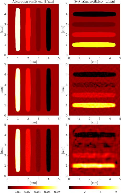
Figure 1: Reconstructed absorption (left column) and scattering (right column) distributions. Rows from top to bottom: simulated true values (first row), reconstructions from data with $0.1\,\%$ of additive noise (second row) and reconstructions from data with $1\,\%$ of additive noise (third row).

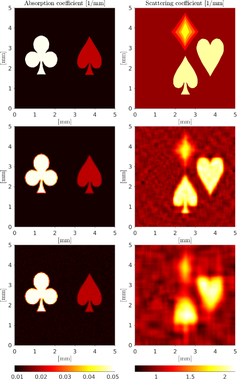
Figure 2: Reconstructed absorption (left column) and scattering (right column) distributions. Rows from top to bottom: simulated true values (first row), reconstructions from data with $0.1\,\%$ of additive noise (second row) and reconstructions from data with $1\,\%$ of additive noise (third row).

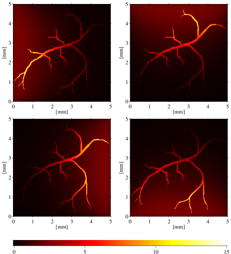
Figure 3: Reconstructed initial pressure distributions (arbitrary units) for the four illuminations of the ’vessel’ target. Reconstructions shown for illumination originating from the left (top left), top (top right), right (bottom left), and bottom (bottom right).

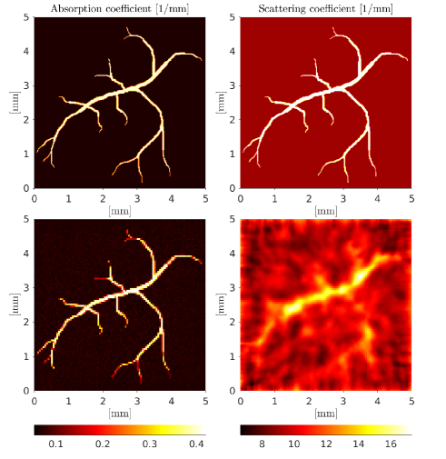
Figure 4: Reconstructed absorption (left column) and scattering (right column) distributions. Simulated true values (top row) and reconstructions from data with $1\,\%$ of additive noise (bottom row).

The relative errors of the estimates computed using Eq. (22) are given in Table 2. As can be seen, the quantitative accuracy of the absorption estimates is good for all tests. The relative errors are approximately on the same level for both ’bars’ and ’cards’ tests with the same amount of additive noise with lowest error of $0.2\,\%$ obtained with ’cards’ test with $0.1\,\%$ of noise and highest error of $2.2\,\%$ obtained with ’bars’ test with $1\,\%$ of noise. The relative errors of scattering are larger, and only in the ’cards’ test with lower amount of additive noise the error is below $10\,\%$. In the case of the ’vessel’ simulation, the relative errors of both absorption and scattering are slightly larger than in the other simulations.

Table 2: Number of iterations needed to reach convergence of the reconstruction algorithm and the relative errors of the absorption $E_{\mu_{\mathrm{a}}}(\%)$ and scattering $E_{\mu_{\mathrm{s}}}(\%)$ estimates evaluated using Eq. (22) in different simulations.

Target	Noise level (%)	Iterations	$E_{\mu_{\mathrm{a}}}(\%)$	$E_{\mu_{\mathrm{s}}}(\%)$
’bars’ (Fig. 1)	0.1	18	0.3	11
’bars’ (Fig. 1)	1.0	10	2.2	20
’cards’ (Fig. 2)	0.1	9	0.2	6.1
’cards’ (Fig. 2)	1.0	7	1.9	11
’vessel’ (Fig. 4)	1.0	10	5.5	20

The computations were performed on a computer with two Intel(R) Xeon(R) Gold 6136 processors with a total of $24$ cores and $256\,{\rm GB}$ of system memory. The reconstructions took about $150$ minutes per step, out of which $20$–$30$ minutes was spent outside of PMC computation (e.g. in the line search and matrix inversions) for the ’bars’ and ’cards’. For the ’vessel’ simulation, the reconstruction times were longer due to the higher scattering of the target which resulted in longer Monte Carlo simulation times. This time consuming nature was eased by reducing the number of photon packets which still remained large enough to maintain the numerical accuracy of the method. Since it took from 10 to 30 steps to reach convergence (see Table 2) and larger discretization is needed in a realistic geometry, the computation times are long for practical applications. However, the photon counts were based on a simple criterion and not optimized. Moreover, the method is trivially parallelizable and easy to implement. Therefore, it seems plausible that implementations using e.g. GPU and adaptive meshing could well succeed in reducing the computation time by orders of magnitude. A systematic study of the quantitative accuracy of the reconstructions as a function of photon packet count remains future work.

4 Conclusion

In this work, a perturbation Monte Carlo method was introduced for the optical inverse problem of quantitative photoacoustic tomography. Bayesian framework was used for the formulation of the inverse problem resulting in a minimization problem that was solved using the Gauss-Newton method. In the proposed approach, Monte Carlo was used as a forward model and perturbation Monte Carlo was used to evaluate the Jacobian matrices for the absorbed optical energy density with respect to the optical absorption and scattering. Evaluation of both the forward model and the Jacobians can be implemented in a simultaneous fashion. Although Bayesian framework was utilised in this work, the perturbation Monte Carlo is not limited to that. It can be utilized similarly with regularization approaches and with different prior models. Future work includes extending the method to three dimensions. In addition, evaluating efficient ways to implement perturbation Monte Carlo using graphics processing units (GPU) should be sought as the approach is (at least in principle) trivially parallelizable. However, potential pitfalls with the GPUs can include inefficient memory usage or unideal parallelization efficiency. Furthermore, the method should be evaluated with experimental data.

Appendix A Perturbation Monte Carlo

To simulate energy absorption $E$ into a domain (or in general to approximate the solution of the RTE [31]), one integrates a function $g$ of a trajectory $s$ over probability distribution function (PDF) of $f$

$$E=\int_{S}g(s)f(s){\rm d}s$$ (23)

where $g(s)$ describes energy absorption and $S$ the ’space’ of all photon trajectories. According to the law of large numbers,

$$\sum_{n=1}^{N}g(s_{n})\to E,\quad{\rm when}\quad N\to\infty$$ (24)

and $s_{n}$ are samples drawn from $f$.

In case we would want to use another PDF $\tilde{f}$ instead, we can obtain these by ’correcting’ samples drawn from $f$ by weighting, and write Eq. (23) as

$$E=\int_{S}g(s)\tilde{f}(s){\rm d}s=\int_{S}g(s)\frac{\tilde{f}(s)}{f(s)}f(s){\rm d}s$$ (25)

and similarly as in the approximation (24) we can write

$$\sum_{n=1}^{N}g(s_{n})\frac{\tilde{f}(s_{n})}{f(s_{n})}\to E,\quad{\rm when}\quad N\to\infty$$ (26)

where $s_{n}$ are samples drawn from $f$.

Considering a photon trajectory consisting of multiple steps with a scattering distance $L_{i}$, a modified weight $\tilde{w}$ utilizing photon trajectories in perturbed and unperturbed regions can be derived

$$\tilde{w}=w\left(\frac{\tilde{\mu}_{\rm s}}{\mu_{\rm s}}\right)^{k}\exp\left[-\left({\tilde{\mu}}_{\rm s}-\mu_{\rm s}\right)L_{\rm tot}\right]$$ (27)

where $w$ is the weight of an unperturbed simulation, $L_{\rm tot}$ is the total trajectory inside the perturbed region and $k$ the number of scattering events in the perturbed region. The correction factor to the weight is the ratio of the PDFs as indicated by Eq. (26). An example for a piece-wise domain is outlined in Fig. 5. Eq. (27) is valid for any range of perturbation. However, in optically challenging simulations, the variance of the Monte Carlo simulation can increase and an increased number of photon packets may be required to reach an acceptable level of noise.

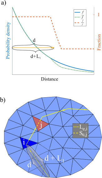
Figure 5: a) Example PDFs for determining the first scattering length in the original ($f$) and perturbed simulation ($\tilde{f}$) for a domain with a piece-wise constant scattering coefficient. Shown is also their ratio that determines the correction factor. b) Domain geometry for the PDFs. Shown is also an exemplar path of a packet. Note that the PDFs are only valid for the first line in the path. The index of the perturbed region is $i$ and the region in which the energy density is evaluated $j$. The length traversed in $i$ before entrance to $j$ is given by $L_{e,i}$, and the length traversed in $j$ by $S_{e,j}$. The number of scattering events in the perturbed region is 1 ($k_{e,i}=1$).

Now, in QPAT in a perturbed medium with piece-wise constant optical coefficients $\mu_{{\rm a},i}$ and $\mu_{{\rm s},i}$, the total optical energy density $\tilde{H}_{j}$ deposited to discretization element $j$ is (c.f. Eq. (16))

$$\tilde{H}_{j}=\frac{1}{A_{j}}\sum_{{{e}}}\tilde{w}_{e}(w_{e},\tilde{\mu}_{{\rm s},i},k_{{e},i},L_{{e},i})\left(1-\exp\left[-\mu_{{\rm a},j}S_{{e},j}\right]\right)$$ (28)

where $k_{{e},i}$ is the number of scattering events and $L_{{e},i}$ is the photon trajectory in the perturbed element $i$ (see Fig. 5). Further, $S_{e,j}$ is the distance traveled on each entrance in element $j$ and $A_{j}$ is the area/volume of the element in 2D/3D. The summation over index $e$ refers to each entrance, including revisits, by the photon packet to the element.

Appendix B Construction of Jacobian

The derivative for the absorption coefficient can be computed directly from Eq. (16) by differentation, but all occurences of $\mu_{\rm a,i}$ must be made explicit since they are only implicitly affecting $w_{e}$. This results in

$$H_{j}=\frac{1}{A_{j}}\sum_{{{e}}}w_{{e}^{\prime}}\exp\left[-\mu_{\rm a,i}L_{{e},i}\right]\left(1-\exp\left[-\mu_{\rm a,j}S_{{e},j}\right]\right)$$ (29)

where $w_{{e}^{\prime}}$ is the weight before entrance to the $j$:th element without the contribution from the $i$:th element, and $L_{{e},i}$ is the distance traveled in element $i$ before each entrance. For $i\neq j$, differentation gives

$$\left(\frac{\partial H_{j}}{\partial\mu_{{\rm a},i}}\right)_{i\neq j}=\frac{1}{A_{j}}\sum_{e}-L_{{e},i}w_{e}\left(1-\exp\left[-\mu_{{\rm a},j}S_{{e},i}\right]\right)$$ (30)

where $w_{e}$ contains the contribution that was excluded from $w_{{e}^{\prime}}$ in Eq. (29). If $i=j$,

$$\begin{split}\frac{\partial H_{j}}{\partial\mu_{{\rm a},j}}=&\frac{1}{A_{j}}\sum_{e}w_{e}\left(L_{e,i}\left(\exp\left[-\mu_{{\rm a},j}S_{{e},j}\right]-1\right)\right.\\ &\left.+S_{{e},j}\exp\left[-\mu_{{\rm a},i}S_{{e},j}\right]\right).\end{split}$$ (31)

For construction of the Jacobian for the scattering, perturbation Monte Carlo is utilized. Then, the derivative with respect to the scattering coefficient can be computed using Eqs. (27) and (28). An analytical expression for $\frac{\partial H_{j}}{\partial\mu_{{\rm s},i}}$ is obtained by writing the difference quotient and taking the limit ${\tilde{\mu}_{{\rm s},i}-\mu_{{\rm s},i}\rightarrow 0}$

$$\begin{split}\frac{\partial H_{j}}{\partial{\mu_{{\rm s},i}}}=&\lim_{\tilde{\mu}_{{\rm s},i}-\mu_{{\rm s},i}\rightarrow 0}\frac{\tilde{H}_{j}-H_{j}}{\tilde{\mu}_{{\rm s},i}-\mu_{{\rm s},i}}\\ =&\lim_{\Delta\mu_{{\rm s},i}\rightarrow 0}\frac{\Delta H_{j}}{\Delta\mu_{{\rm s},i}}\\ =&\frac{1}{A_{j}}\lim_{\Delta\mu_{\rm s,i}\rightarrow 0}\frac{1}{\Delta\mu_{{\rm s},i}}\left(\sum_{{e}}w_{e}\left(\frac{\mu_{{\rm s},i}+\Delta\mu_{{\rm s},i}}{\mu_{{\rm s},i}}\right)^{k_{{e},i}}\right.\\ &\cdot\exp\left[{-\Delta\mu_{{\rm s},i}L_{{e},i}}\right]\left(1-\exp\left[-\mu_{{\rm a},j}S_{e,j}\right]\right)\\ &\left.-\sum_{{e}}w_{e}\left(1-\exp\left[{-\mu_{{\rm a},j}S_{{e},j}}\right]\right)\right)\end{split}$$ (32)

The limit can be evaluated using the first order expansions for two the expressions in the numerator with $\Delta\mu_{{\rm s},i}$ to obtain

$$\begin{split}\frac{\partial H_{j}}{\partial{\mu_{{\rm s},i}}}=&\frac{1}{A_{j}}\sum_{e}w_{e}\left(\frac{k_{{e},i}}{\mu_{{\rm s},i}}-L_{{e},i}\right)\\ &\cdot\left(1-\exp\left[-\mu_{{\rm a},j}S_{{e},j}\right]\right).\end{split}$$ (33)

Computation of the Jacobian was validated with simulations described in Appendix C.

Appendix C Validation of the Jacobian computation

Computation of the Jacobian was validated by evaluating derivatives of absorption and scattering, Eqs. (19), (20) and (21), and comparing them to a least-squares estimation of the derivatives from a finite difference approximation utilizing conventional Monte Carlo simulations. A simple rectangular test geometry of size $3\,{\rm mm}\times 3\,{\rm mm}$ that was discretized into $81$ pixels was used. The absorption and scattering coefficients of each pixel were selected at random in the intervals $\mu_{\mathrm{a}}\in[0\,,\,0.05]\,{\rm mm}^{-1}$ and $\mu_{\mathrm{s}}\in[0\,,\,3]\,{\rm mm}^{-1}$. Scattering anisotropy was selected as a constant value for the whole simulation domain randomly in the interval of $g\in[-0.8\,,\,0.8]$.

The derivatives using the least squares approach were computed as follows. First two random pixels $i$ and $j$ were selected. Symbol $i$ stands for the pixel in which the absorbed energy is evaluated and $j$ for the pixel where the optical coefficient is varied. Then, to evaluate e.g. the derivative for absorption $J_{i,j}=\frac{\partial E_{i}}{\partial\mu_{{\rm a},j}}$, we introduced a small random variation $\delta\mu_{\mathrm{a}}$ to $\mu_{{\rm a},j}$ into the absorption coefficient of the pixel $j$ several times and computed the energy absorbed in the pixel $i$ using Monte Carlo. Since $\delta\mu_{\mathrm{a}}$ is small, a least-squares line can be fitted to these values to estimate the derivative from the slope. Derivatives with respect to the scattering coefficient were evaluated in the same way.

All the derivatives produced in this way agreed to those computed using Eqs. (19), (20) and (21). The photon count and the magnitude of the varied parameters were improved (i.e. increasing photon count and decreasing the magnitude) until the results agreed within $95\,\%$ confidence. However, the numerical noise in the data for the least-squares estimate sometimes became too high to obtain good enough relative accuracy for comparison. Generally, this tends to happen if the distance between the pixels $i$ and $j$ is large. An example of evaluating scattering derivatives using two pixels located at a distance of $0.67\,{\rm mm}$ from each other is shown in Fig. 6. In general, the simulations showed a good agreement between the derivatives evaluated using the two approaches.

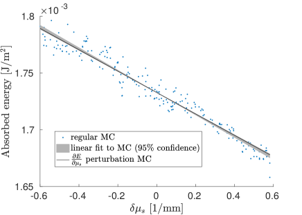
Figure 6: Energy absorbed to one pixel of a rectangular simulation domain of size $3\,{\rm mm}\times 3\,{\rm mm}$ at a distance of $0.67\,{\rm mm}$ from another pixel where scattering was varied, a linear fit for determining the slope $\frac{\partial E}{\partial\mu_{\mathrm{s}}}$ (grey region), and a line with a slope that is estimated at $\delta\mu_{\mathrm{s}}=0$ using perturbation Monte Carlo (black line).

References

- [1] M. Xu and L. V. Wang, “Photoacoustic imaging in biomedicine,” Rev. Sci. Instrum., vol. 77, p. 041101, 2006.
- [2] C. Li and L. V. Wang, “Photoacoustic tomography and sensing in biomedicine,” Phys. Med. Biol., vol. 54, pp. R59–R97, 2009.
- [3] L. V. Wang, Ed., Photoacoustic Imaging and Spectroscopy. CRC Press, 2009.
- [4] P. Beard, “Biomedical photoacoustic imaging,” Interface Focus, vol. 1, pp. 602–631, 2011.
- [5] J. Xia and L. V. Wang, “Small-animal whole-body photoacoustic tomography: a review,” Phys. Med. Biol., vol. 61, no. 5, pp. 1380–1389, 2014.
- [6] L. V. Wang and J. Yao, “A practical guide to photoacoustic tomography in the life sciences,” Nat. Methods, vol. 13, no. 8, pp. 627–638, 2016.
- [7] J. Weber, P. C. Beard, and S. Bohndiek, “Contrast agents for molecular photoacoustic imaging,” Nat. Methods, vol. 13, no. 8, pp. 639–650, 2016.
- [8] J. Brunker, J. Yao, J. Laufer, and S. E. Bohndiek, “Photoacoustic imaging using genetically encoded reporters: a review,” J. Biomed. Opt., vol. 22, no. 7, p. 070901, 2017.
- [9] B. Cox, J. G. Laufer, S. R. Arridge, and P. C. Beard, “Quantitative spectroscopic photoacoustic imaging: a review,” J. Biomed. Opt., vol. 17, no. 6, p. 061202, 2012.
- [10] A. Ishimaru, Wave Propagation and Scattering in Random Media. New York: Academic Press, 1978, vol. 1.
- [11] S. R. Arridge, “Optical tomography in medical imaging,” Inv. Probl., vol. 15, pp. R41–R93, 1999.
- [12] S. A. Prahl, M. Keijzer, S. L. Jacques, and A. J. Welch, “A Monte Carlo model of light propagation in tissue,” in Proc. SPIE, Dosimetry of Laser Radiation in Medicine and Biology, G. Müller and D. Sliney, Eds., vol. IS 5, 1989, pp. 102–111.
- [13] L. Wang, S. Jacques, and L. Zheng, “MCML – Monte Carlo modeling of photon transport in multi-layered tissues,” Comput. Methods Programs Biomed., vol. 47, pp. 131–146, 1995.
- [14] A. Sassaroli and F. Martelli, “Equivalence of four Monte Carlo methods for photon migration in turbid media,” J. Opt. Soc. Am. A, vol. 29, no. 10, pp. 2110–2117, 2012.
- [15] C. Zhu and Q. Liu, “Review of Monte Carlo modeling of light transport in tissues,” J. Biomed. Opt., vol. 18, no. 5, p. 050902, 2013.
- [16] C. Hayakawa, J. Spanier, and V. Venugopalan, “Comparative analysis of discrete and continuous absorption weighting estimators used in Monte Carlo simulations of radiative transport in turbid media,” J. Opt. Soc. Am. A, vol. 31, no. 2, pp. 301–311, 2014.
- [17] Q. Fang and D. Boas, “Monte Carlo simulation of photon migration in 3D turbid media accelerated by graphics processing units,” Opt. Express, vol. 17, no. 22, pp. 20 178–20 190, 2009.
- [18] O. Yang and B. Choi, “Accelerated rescaling of single Monte Carlo simulation runs with the Graphics Processing Unit (GPU),” Biomed. Opt. Express, vol. 4, no. 11, pp. 2667–2672, 2013.
- [19] J. Cassidy, A. Nouri, V. Betz, and L. Lilge, “High-performance, robustly verified Monte Carlo simulation with FullMonte,” J. Biomed. Opt., vol. 23, no. 8, p. 085001, 2018.
- [20] Y. Liu, S. Jacques, M. Azimipour, J. Rogers, R. Pashaie, and K. Eliceiri, “OptogenSIM: a 3D Monte Carlo simulation platform for light delivery design in optogenetics,” Biomed. Opt. Express, vol. 6, no. 12, pp. 4859–4870, 2015.
- [21] A. A. Leino, A. Pulkkinen, and T. Tarvainen, “ValoMC: a Monte Carlo software and MATLAB toolbox for simulating light transport in biological tissue,” OSA Continuum, vol. 2, no. 3, pp. 957–972, Mar 2019.
- [22] T. Tarvainen, B. T. Cox, J. P. Kaipio, and S. R. Arridge, “Reconstructing absorption and scattering distributions in quantitative photoacoustic tomography,” Inv. Probl., vol. 28, p. 084009, 2012.
- [23] T. Saratoon, T. Tarvainen, B. T. Cox, and S. R. Arridge, “A gradient-based method for quantitative photoacoustic tomography using the radiative transfer equation,” Inv. Probl., vol. 29, p. 075006, 2013.
- [24] A. V. Mamonov and K. Ren, “Quantitative photoacoustic imaging in radiative transport regime,” Comm. Math. Sci., vol. 12, pp. 201–234, 2014.
- [25] M. Haltmeier, L. Neumann, and S. Rabanser, “Single-stage reconstruction algorithm for quantitative photoacoustic tomography,” Inv. Probl., vol. 31, p. 065005, 2015.
- [26] J. Buchmann, B. A. Kaplan, S. Prohaska, and J. Laufer, “Experimental validation of a Monte-Carlo-based inversion scheme for 3D quantitative photoacoustic tomography,” in Photons Plus Ultrasound: Imaging and Sensing 2017, Proc of SPIE, A. Oraevsky and L. Wang, Eds., vol. 10064, 2017, p. 1006416.
- [27] B. A. Kaplan, J. Buchmann, S. Prohaska, and J. Laufer, “Monte-Carlo-based inversion scheme for 3D quantitative photoacoustic tomography,” in Photons Plus Ultrasound: Imaging and Sensing 2017, Proc of SPIE, A. Oraevsky and L. Wang, Eds., vol. 10064, 2017, p. 100645J.
- [28] R. Hochuli, S. Powell, S. Arridge, and B. Cox, “Quantitative photoacoustic tomography using forward and adjoint Monte Carlo models of radiance,” J Biomed Opt, vol. 21, no. 12, p. 126004, 2016.
- [29] J. Buchmann, B. A. Kaplan, S. Powell, S. Prohaska, and J. Laufer, “Three-dimensional quantitative photoacoustic tomography using an adjoint radiance Monte Carlo model and gradient descent,” J. Biomed. Opt., vol. 24, no. 6, p. 066001, 2019.
- [30] J. Buchmann, B. Kaplan, S. Powell, S. Prohaska, and J. Laufer, “Quantitative PA tomography of high resolution 3-D images: experimental validation in a tissue phantom,” Photoacoustics, vol. 17, p. 100157, 2020.
- [31] I. Lux and L. Koblinger, Monte Carlo Particle Transport Methods: Neutron and Photon Calculations. CRC Press, 1991.
- [32] A. Kienle and M. S. Patterson, “Determination of the optical properties of turbid media from a single Monte Carlo simulation,” Phys. Med. Biol., vol. 41, pp. 2221-2227, 1996.
- [33] A. Pifferi, P. Taroni, G. Valentini, and S. Andersson-Engels, “Real-time method for fitting time-resolved reflectance and transmittance measurements with a Monte Carlo model,” Appl. Opt., vol. 37, no. 13, pp. 2774-2780, 1998.
- [34] C. K. Hayakawa, J. Spanier, F. Bevilacqua, A. K. Dunn, J. S. You, B. J. Tromberg et al., “Perturbation Monte Carlo methods to solve inverse photon migration problems in heterogeneous tissues,” Opt. Lett., vol. 26, no. 17, pp. 1335–1337, Sep 2001.
- [35] Y. Kumar and R. Vasu, “Reconstruction of optical properties of low-scattering tissue using derivative estimated through perturbation Monte-Carlo method,” J. Biomed. Opt., vol. 9, no. 5, pp. 1002–1012, 2004.
- [36] E. Alerstam, S. Andersson-Engels, and T. Svensson “White Monte Carlo for time-resolved photon migration,” J. Biomed. Opt., vol. 13, no. 4, p. 041304, 2008.
- [37] J. Chen and X. Intes, “Time-gated perturbation Monte Carlo for whole body functional imaging in small animals,” Opt. Express., vol. 17, no. 22, pp. 19 566–19 579, 2009.
- [38] A. Sassaroli, “Fast perturbation Monte Carlo method for photon migration in heterogeneous turbid media,” Opt. Lett., vol. 36, no. 11, pp. 2095–2097, 2011.
- [39] X. Zhang, “Construction of the Jacobian matrix for fluorescence diffuse optical tomography using a perturbation Monte Carlo method,” in Multimodal Biomedical Imaging VII, Proc. of SPIE, vol. 8216, 2012, p. 82160O.
- [40] T. Yamamoto and H. Sakamoto, “Frequency domain optical tomography using a Monte Carlo perturbation method,” Opt. Comm., vol. 364, pp. 165–176, 2016.
- [41] R. Yao, X. Intes, and Q. Fang, “Direct approach to compute Jacobians for diffuse optical tomography using perturbation Monte Carlo-based photon ”replay”,” Biomed. Opt. Express, vol. 9, no. 10, pp. 4588–4603, 2018.
- [42] L. G. Henyey and J. L. Greenstein, “Diffuse radiation in the galaxy,” AstroPhys. J., vol. 93, pp. 70–83, 1941.
- [43] B. T. Cox and P. C. Beard, “Fast calculation of pulsed photoacoustic fields in fluids using k-space methods,” J. Acoust. Soc. Am., vol. 117, no. 6, pp. 3616–3627, 2005.
- [44] B. E. Treeby and B. T. Cox, “k-Wave: MATLAB toolbox for the simulation and reconstruction of photoacoustic wave fields,” J. Biomed, Opt., vol. 15, no. 2, p. 021314, 2010.
- [45] J. Kaipio and E. Somersalo, Statistical and Computational Inverse Problems. New York: Springer, 2005.
- [46] T. Tarvainen, A. Pulkkinen, B. T. Cox, J. P. Kaipio, and S. R. Arridge, “Bayesian image reconstruction in quantitative photoacoustic tomography,” IEEE Trans. Med. Imag., vol. 32, no. 12, pp. 2287–2298, 2013.
- [47] C. E. Rasmussen and C. K. I. Williams, Gaussian Processes for Machine Learning. MIT Press, 2006.
- [48] A. Pulkkinen, B. T. Cox, S. R. Arridge, J. P. Kaipio, and T. Tarvainen, “A Bayesian approach to spectral quantitative photoacoustic tomography,” Inv. Probl., vol. 30, p. 065012, 2014.
- [49] J. Nocedal and S. Wright, Numerical Optimization. Springer, 2006.
- [50] S. Jacques, “Optical properties of biological tissues: a review,” Phys. Med. Biol., vol. 58, no. 11, pp. R37–R61, 2013.
- [51] M. Friebel, A. Roggan, G. Müller, and M. Meinke, “Determination of optical properties of human blood in the spectral range 250 to 1100 nm using Monte Carlo simulations with hematocrit-dependent effective scattering phase functions,” J Biomed. Opt., vol. 11, no. 3, p. 034021, 2006.
- [52] J. Schöberl, “NETGEN An advancing front 2D/3D-mesh generator based on abstract rules,” Comput. Vis. Sci., vol. 1, no. 1, pp. 41–52, 1997.
- [53] E. Zhang, J. Laufer, and P. Beard, “Backward-mode multiwavelength photoacoustic scanner using a planar Fabry-Perot polymer film ultrasound sensor for high-resolution three-dimensional imaging of biological tissues,” Appl. Opt., vol. 47, no. 4, pp. 561–577, 2008.
- [54] J. Buchmann, E. Zhang, C. Scharfenorth, B. Spannekrebs, C. Villringer, and J. Laufer, ”Evaluation of Fabry-Perot polymer film sensors made using hard dielectric mirror deposition”, in Photons Plus Ultrasound: Imaging and Sensing 2017, Proc of SPIE, A. Oraevsky and L. Wang, Eds., vol. 9708, 2016, p. 970856.
- [55] R. Ellwood, O. Ogunlade, E. Zhang, P. Beard, and B. Cox, “Photoacoustic tomography using orthogonal Fabry-Pérot sensors,” J. Biomed. Opt., vol. 22, no. 4, p. 041009, 2017.