The Virtual Element Method
for a Minimal Surface Problem

Abstract

In this paper we consider the Virtual Element discretization of a minimal surface problem, a quasi-linear elliptic partial differential equation modeling the problem of minimizing the area of a surface subject to a prescribed boundary condition. We derive optimal error estimate and present several numerical tests assessing the validity of the theoretical results.

1 Introduction

In recent years, the numerical approximation of partial differential equations on computational meshes composed by arbitrarily-shaped polygonal/polyhedral (polytopal, for short) elements has been the subject of an intense research activity. Examples of such methods include the Mimetic Finite Difference method, the Polygonal Finite Element Method, the polygonal Discontinuous Galerkin Finite Element Methods, the Hybridizable Discontinuous Galerkin and Hybrid High-Order Methods, the Gradient Discretization method, the Finite Volume Method, the BEM-based FEM, the Weak Galerkin method and the Virtual Element method (VEM). For more details see the special issue [6] and the references therein. VEM has been introduced in [10] for elliptic problems and later extended to several different linear and non-linear differential problems. While the analysis of linear problems is much more flourished, the study of Virtual Element discretization for non-linear problems is much less developed (see, e.g., [4, 15, 11, 9, 5, 7, 12, 20, 3, 2, 1, 17]). In this paper we contribute to fill this gap by addressing the (lowest order) Virtual Element discretization of a minimal surface problem (see, e.g., [13] for its finite element discretization). More precisely, in Section 2 we introduce the continuous problem together with its Virtual Element discretization, while in Section 3 we derive optimal error estimate in the $H^{1}$-norm, under a condition on the discrete solution, the validity of which can be checked “a posteriori”. Finally, in Section 4 we present several numerical results assessing the validity of the theoretical estimate and confirming that optimal convergence is indeed achieved. Moreover, the convergence properties in the $L^{2}$-norm is numerically investigated.

1.1 Notation

Throughout the paper we shall use the standard notation of the Sobolev spaces $H^{m}(\mathcal{D})$ for a nonnegative integer $m$ and an open bounded domain $\mathcal{D}$. The $m$-th seminorm of the function $v$ will be denoted by

$$|v|{{}^{2}}_{m,\mathcal{D}}=\sum_{|\alpha|=m}\bigg{\|}\frac{\partial^{|\alpha|}v}{\partial_{x_{1}}^{\alpha_{1}}\partial_{x_{2}}^{\alpha_{2}}}\bigg{\|}^{2}_{0,\mathcal{D}},$$

where $\|\cdot\|_{0,\mathcal{D}}$ stands for the $L^{2}(\mathcal{D})$ norm and we set $|{\alpha}|=\alpha_{1}+\alpha_{2}$ for the nonnegative multi-index ${\alpha}=(\alpha_{1},\alpha_{2})$. For any integer $m\geq 0$, $\mathbb{P}^{m}({\mathcal{D}})$ is the space of polynomials of total degree up to $m$ defined on ${\mathcal{D}}$. Moreover, $n=(n_{1},n_{2})$ is the outward unit normal vector to $\partial\mathcal{D}$, the boundary of $\mathcal{D}$. Finally, we will employ the symbol $\lesssim$ for an inequality holding up to a constant independent of the mesh size.

2 Continuous problem and its VEM discretization

Let $\Omega\subseteq\mathbb{R}^{2}$ be a bounded open set. In the following, we will employ the following notation

$$f(\cdot)=\sqrt{1+|\nabla(\cdot)|^{2}}.$$

Let $\varphi$ be a function given on the boundary $\Gamma=\partial\Omega$. The minimal surface problem amounts to finding a function $u$ which minimizes the functional

$$J(v)=\int_{\Omega}f(v)dx$$

over a suitable space of functions which are equal to $\varphi$ on $\Gamma$. The existence and uniqueness of a solution is a delicate mathematical issue (see, e.g., [13] and the references therein). Here, with the aim of simplifying the analysis, we follow the framework considered, e.g., in [13] and make the following hypotheses: the domain $\Omega$ is a convex polygonal set and the function $\varphi$ is the trace over $\Gamma$ of a function (by abuse of notation still denoted by $\varphi$) of $H^{2}(\Omega)$. Moreover, for the subsequent discussion, as in [13], we consider that the minimal surface problem consists in solving the following:

$$u=\mathop{\mathrm{arg\,min}}_{v\in V^{\varphi}}J(v),$$ (1)

where $V^{\varphi}=\{v\in H^{1}(\Omega):~{}u=\varphi\text{~{}on~{}}\partial\Omega\}$. Note that $u$ is the solution to (1) if and only if $u\in V^{\varphi}$ solves

$$\int_{\Omega}\frac{\nabla u\cdot\nabla v}{f(u)}=0\qquad\forall v\in V^{0}=H^{1}_{0}(\Omega).$$ (2)

Let $\{\mathcal{T}_{h}\}_{h}$ be a sequence of decompositions (meshes) of $\Omega$ into non-overlapping polygons $E$. Each mesh $\mathcal{T}_{h}$ is labeled by the mesh size parameter $h$, which will be defined below, and satisfies suitable regularity assumptions that are customarily made to prove the convergence of the method and derive an estimate of the approximation error. These regularity assumptions are introduced and discussed in Section 3. Let $\mathcal{E}_{h}$ be the set of edges of $\mathcal{T}_{h}$ such that $\mathcal{E}_{h}=\mathcal{E}_{h}^{i}\cup\mathcal{E}_{h}^{\Gamma}$, where $\mathcal{E}_{h}^{i}$ and $\mathcal{E}_{h}^{\Gamma}$ are the set of interior and boundary edges, respectively. Similarly, we denote by $V_{h}=V_{h}^{i}\cup V_{h}^{\Gamma}$ the set of vertices in $\mathcal{T}_{h}$, where $V_{h}^{i}$ and $V_{h}^{\Gamma}$ are the sets of interior and boundary vertices, respectively. Accordingly, $V_{h}^{E}$ is the set of vertices of $E$. Moreover, $|E|$ and $|e|$ denote the area of cell $E$ and the length of edge $e$, respectively, $\partial E$ is the boundary of $E$, $h_{E}$ is the diameter of $E$ and the mesh size parameter is defined as $h=\max_{E\in\mathcal{T}_{h}}h_{E}$.

Let us introduce the usual local lowest order conforming Virtual Element space on the polygon $E$ (see, e.g., [10])

$$V^{E}_{h}=\{v_{h}\in H^{1}(E):~{}\Delta v_{h}=0\text{~{}in~{}}E,~{}v_{h}\in C^{0}(\partial E),v_{h}|_{e}\in\mathbb{P}^{1}(e)~{}\forall e\in\partial E\},$$

where, for $D$ $d$-dimensional domain, $\mathbb{P}^{1}(D)$ denotes the space of $d$-variate polynomials of order less than or equal to one on $D$. Accordingly, the global Virtual Element space is defined as follows

$$V_{h}^{\varphi}=\{v_{h}\in H^{1}(\Omega):~{}v_{h}|_{E}\in V_{h}^{E},~{}v_{h}(V)=\varphi(V)~{}\text{~{}for~{}each~{}vertex~{}V}\in V_{h}^{\Gamma}\}.$$

Consistently, we denote by $V_{h}^{0}$ the global VEM space with homogeneous Dirichlet boundary conditions.

Let $S^{E}(\cdot,\cdot)$ be the usual stabilization term employed for constructing the VEM discretization of the Laplace problem, i.e. the Euclidean scalar product associated with the degrees of freedom (here the vertex values). See, e.g., [10, 8] for further details. Moreover, let $\Pi^{\nabla}_{E}\colon V^{E}_{h}\rightarrow\mathbb{P}^{1}(E)$ the usual elliptic projection operator (see, e.g., [10]).

We introduce the local discrete function $f^{E}_{h}:V^{E}_{h}\to\mathbb{R}$ defined as

$$f^{E}_{h}(v_{h})=\sqrt{1+|\nabla\Pi^{\nabla}_{E}v_{h}|^{2}+|E|^{-1}S^{E}((I-\Pi^{\nabla}_{E})v_{h},(I-\Pi^{\nabla}_{E})v_{h})}.$$ (3)

Roughly speaking, $f_{h}^{E}(\cdot)$ represents an approximation to $\sqrt{1+|(\nabla\cdot)_{|E}|^{2}}$.

Having in mind the above definitions, the discrete virtual counterpart of the continuous minimization problem (1) reads as follows

$$u_{h}=\mathop{\mathrm{arg\,min}}_{v_{h}\in V_{h}^{\varphi}}J_{h}(v_{h}),\quad\text{ with }\quad J_{h}(v_{h})=\sum_{E\in\mathcal{T}_{h}}\int_{E}f^{E}_{h}(v_{h})\,dx.$$ (4)

Thus, the Virtual Element discretization of (2) is as follows: find $u_{h}\in V_{h}^{\varphi}$ such that

$$A_{h}(u_{h};u_{h},v_{h})=0$$ (5)

for all $v_{h}\in V_{h}^{0}$, where $A_{h}(w_{h};u_{h},v_{h})=\sum_{E}A_{h}^{E}(w_{h};u_{h},v_{h})$ and

$$A_{h}^{E}(w_{h};u_{h},v_{h})=\int_{E}\frac{\nabla\Pi^{\nabla}_{E}u_{h}\cdot\nabla\Pi^{\nabla}_{E}v_{h}}{f^{E}_{h}(w_{h})}\,dx+\frac{S^{E}((I-\Pi^{\nabla}_{E})u_{h},(I-\Pi^{\nabla}_{E})v_{h})}{f^{E}_{h}(w_{h})}.$$ (6)

Note that as $f_{h}^{E}(w_{h})$ is constant on each polygon $E$, the form $A^{E}_{h}(\cdot;\cdot,\cdot)$ can be equivalently written as

$$A_{h}^{E}(w_{h};u_{h},v_{h})=\frac{a_{h}^{E}(u_{h},v_{h})}{f_{h}^{E}(w_{h})}$$ (7)

where

$$a_{h}^{E}(u_{h},v_{h})=\int_{E}\nabla\Pi^{\nabla}_{E}u_{h}\cdot\nabla\Pi^{\nabla}_{E}v_{h}dx+S^{E}((I-\Pi^{\nabla}_{E})u_{h},(I-\Pi^{\nabla}_{E})v_{h})$$

is the classical local discrete VEM bilinear form for the Laplace problem. It is worth remembering (see, e.g., [10]) that $a_{h}^{E}(\cdot,\cdot)$ satisfies the following two crucial properties:

$(i)$

Consistency: for every polynomial $q\in\mathbb{P}^{1}(E)$ and function $v_{h}\in V_{h}^{E}$ we have:

$$a^{E}_{h}(v_{h},q)=a^{E}(v_{h},q);$$ (8)

$(ii)$

Stability: there exist two positive constants $\alpha_{*}$, $\alpha^{*}$ independent of $h$ and $E$ such that for every $v_{h}\in V_{h}^{E}$ it holds:

$$\alpha_{*}a^{E}(v_{h},v_{h})\leq a^{E}_{h}(v_{h},v_{h})\leq\alpha^{*}a^{E}(v_{h},v_{h}).$$ (9)

Remark that requiring that the stability condition $(ii)$ holds is equivalent to requiring that there exists positive constants $\widetilde{\alpha}_{*}$ and $\widetilde{\alpha}^{*}$ such that, for all $v_{h}\in V_{h}^{E}$ with $\Pi^{\nabla}_{E}v_{h}=0$ it holds:

$${\widetilde{\alpha}}_{*}a^{E}(v_{h},v_{h})\leq S^{E}(v_{h},v_{h})\leq{\widetilde{\alpha}}^{*}a^{E}(v_{h},v_{h}),$$ (10)

(see [10] for more details). Existence and uniqueness of the solution $u_{h}\in V_{h}^{\varphi}$ follow by working on the discrete cost functional $J_{h}(v_{h})$ as in [13].

For future use, we set $a^{E}(u_{h},v_{h})=\int_{E}\nabla u_{h}\cdot\nabla v_{h}dx$.

3 Error analysis

We make the following regularity assumptions on the mesh sequence $\{\mathcal{T}_{h}\}_{h}$:

• there exists a constant $\rho_{0}>0$ independent of $\mathcal{T}_{h}$, such that for every element $E$ it holds:

  1. $E$ is star-shaped with respect to all the points of a ball of radius $\rho_{0}h_{E}$

  2. every edge $e\in\mathcal{E}_{h}$ has length $|e|\geq\rho_{0}h_{E}$.

The assumptions (H1)-(H2) are standard (see, e.g.,  [10]) and allow to define, for every smooth enough function $v$, an “interpolant” $v_{I}$ in $V^{\varphi}_{h}$ such that it holds $|v-v_{I}|_{{1,\Omega}}{\lesssim}h$ (see [10]).

We now state the main result of the paper.

Theorem 3.1.

Let $u\in H^{2}(\Omega)\cap W^{1,\infty}(\Omega)$ be the continuous solution to (1), and let $u_{h}\in V_{h}^{\varphi}$ be the VEM solution to (5). Letting

$$C(u_{h})=h^{-1}\sqrt{\sum_{E}S^{E}((I-\Pi_{E}^{\nabla})u_{h},(I-\Pi_{E}^{\nabla})u_{h}),}$$

it holds

$$|u-u_{h}|_{{1,\Omega}}\lesssim(1+C(u_{h}))^{2}h.$$ (11)

Corollary 3.2.

Assume that $C(u_{h})\lesssim 1$. Then it holds that

$$|u-u_{h}|_{{1,\Omega}}\lesssim h.$$

Proof.

By triangle inequality we have

$$|u-u_{h}|_{{1,\Omega}}\leq|u-u_{I}|_{{1,\Omega}}+|u_{I}-u_{h}|_{{1,\Omega}}.$$

In the following, we adapt the ideas of [16] to the present context. We preliminary observe that the following holds true

$$|u_{I}-u_{h}|_{{1,\Omega}} = \left(\sum_{E\in\mathcal{T}_{h}}\int_{E}\frac{|\nabla(u_{I}-u_{h})|^{2}}{f_{h}^{E}(u_{h})}f^{E}_{h}(u_{h})\right)^{1/2}$$ (12)

$$\leq \left(\max_{E}|f^{E}_{h}(u_{h})|\right)^{1/2}\left(\sum_{E\in\mathcal{T}_{h}}\int_{E}\frac{|\nabla(u_{I}-u_{h})|^{2}}{f^{E}_{h}(u_{h})}\right)^{1/2}.$$

The remaining part of the proof is devoted to show:

• $\displaystyle{\left(\sum_{E\in\mathcal{T}_{h}}\int_{E}\frac{|\nabla(u_{I}-u_{h})|^{2}}{f_{h}^{E}(u_{h})}\right)^{1/2}\lesssim(1+C(u_{h}))h}$;

• $\displaystyle{\max_{E}|f^{E}_{h}(u_{h}){|}\lesssim(1+C(u_{h}))^{2}}$.

Let us first prove $(i)$. We start by observing that, thanks to (10), we have

$$|u_{h}-\Pi^{\nabla}_{E}u_{h}|_{1,h}\lesssim C(u_{h})h$$ (13)

where where $|v|_{1,h}^{2}=\sum_{E\in\mathcal{T}_{h}}{\|\nabla v\|_{0,E}^{2}}$. By using the stability property of $a_{h}^{E}(\cdot,\cdot)$, as $f_{h}^{E}(u_{h})$ is constant on $E$, we get the following inequalities with $\delta_{h}=u_{h}-u_{I}$

$$\sum_{E\in\mathcal{T}_{h}}\int_{E}\frac{|\nabla(u_{I}-u_{h})|^{2}}{f_{h}^{E}(u_{h})} \lesssim \sum_{E\in\mathcal{T}_{h}}\frac{a_{h}^{E}(\delta_{h},\delta_{h})}{f_{h}^{E}(u_{h})}$$ (14)

$$\lesssim \left|-\sum_{E\in\mathcal{T}_{h}}\frac{a_{h}^{E}(u_{I},\delta_{h})}{f_{h}^{E}(u_{h})}\right|,$$

where in the last step we employ (5) with $\delta_{h}\in V_{h}^{0}$. Let $u_{\pi}|_{E}$ be the $L^{2}(E)$ projection of $u$ onto $\mathbb{P}^{1}(E)$. By employing the consistency and stability properties of $a_{h}^{E}(\cdot,\cdot)$ together with the fact that $u$ is solution to (1), it is immediate to check that the following holds

$$-\sum_{E\in\mathcal{T}_{h}}\frac{a_{h}^{E}(u_{I},\delta_{h})}{f^{E}_{h}(u_{h})} = -\sum_{E\in\mathcal{T}_{h}}\Bigg{\{}\frac{a_{h}^{E}(u_{I}-u_{\pi},\delta_{h})}{f^{E}_{h}(u_{h})}+\frac{a_{h}^{E}(u_{\pi},\delta_{h})}{f^{E}_{h}(u_{h})}$$

$$\pm\frac{a^{E}(u,\delta_{h})}{f^{E}_{h}(u_{h})}-\int_{E}\frac{\nabla u\cdot\nabla\delta_{h}}{f(u)}dx\Bigg{\}}$$

$$= \sum_{E\in\mathcal{T}_{h}}\frac{a_{h}^{E}(u_{\pi}-u_{I},\delta_{h})}{f^{E}_{h}(u_{h})}+\sum_{E\in\mathcal{T}_{h}}\frac{a^{E}(u-u_{\pi},\delta_{h})}{f^{E}_{h}(u_{h})}$$

$$+\sum_{E\in\mathcal{T}_{h}}\int_{E}\nabla u\cdot\nabla\delta_{h}\left(\frac{1}{f(u)}-\frac{1}{f^{E}_{h}(u_{h})}\right)dx$$

$$= A+B+C.$$ (16)

We now bound the three terms separately. By combining the Cauchy-Schwarz inequality with the fact that $f_{h}^{E}(u_{h})$ is constant and larger than $1$ on each polygon $E$, we have

$$A\leq(|u-u_{\pi}|_{1,h}+|u-u_{I}|_{{1,\Omega}})\left(\sum_{E\in\mathcal{T}_{h}}\int_{E}\frac{|\nabla(u_{I}-u_{h})|^{2}}{f^{E}_{h}(u_{h})}dx\right)^{1/2},$$ (17)

and

$$B\leq|u-u_{\pi}|_{1,h}\left(\sum_{E\in\mathcal{T}_{h}}\int_{E}\frac{|\nabla(u_{I}-u_{h})|^{2}}{f^{E}_{h}(u_{h})}dx\right)^{1/2}.$$ (18)

Finally, setting $\gamma=\max_{\bar{\Omega}}\frac{|\nabla u|}{f(u)}$, employing the definitions of $f(\cdot)$ and $f^{E}_{h}(\cdot)$ and observing that $f(u)\geq|\nabla u|$, the following holds

$$C = \sum_{E\in\mathcal{T}_{h}}\int_{E}\nabla u\cdot\nabla\delta_{h}\frac{[f_{h}^{E}(u_{h})]^{2}-f^{2}(u)}{f(u)f_{h}^{E}(u_{h})(f(u)+f_{h}^{E}(u_{h}))}dx$$

$$\leq \gamma\sum_{E\in\mathcal{T}_{h}}\int_{E}|\nabla\delta_{h}|\frac{|f^{2}(u)-[f_{h}^{E}(u_{h})]^{2}|}{f_{h}^{E}(u_{h})(f(u)+f_{h}^{E}(u_{h}))}dx$$

$$= \gamma\sum_{E\in\mathcal{T}_{h}}\Bigg{\{}\int_{E}|\nabla\delta_{h}|\frac{\left||\nabla u|^{2}-|\nabla\Pi_{E}^{\nabla}u_{h}|^{2}\right|}{f_{h}^{E}(u_{h})(f(u)+f_{h}^{E}(u_{h}))}dx$$

$$+\int_{E}|\nabla\delta_{h}|\frac{|E|^{-1}S^{E}((I-\Pi_{E}^{\nabla})u_{h},(I-\Pi_{E}^{\nabla})u_{h}))}{f_{h}^{E}(u_{h})(f(u)+f_{h}^{E}(u_{h}))}dx\Bigg{\}}=C.I+C.II$$

As $f_{h}^{E}(u_{h})\geq|\nabla\Pi_{E}^{\nabla}u_{h}|$, we can bound

$$C.I = \gamma\sum_{E\in\mathcal{T}_{h}}\int_{E}|\nabla\delta_{h}|\frac{\left||\nabla u|^{2}-|\nabla\Pi_{E}^{\nabla}u_{h}|^{2}\right|}{f_{h}^{E}(u_{h})(f(u)+f_{h}^{E}(u_{h}))}dx$$

$$\leq \gamma\sum_{E\in\mathcal{T}_{h}}\int_{E}|\nabla\delta_{h}|\frac{|\nabla(u-\Pi_{E}^{\nabla}u_{h})|(|\nabla u|+|\nabla\Pi_{E}^{\nabla}u_{h}|)}{f_{h}^{E}(u_{h})(f(u)+f_{h}^{E}(u_{h}))}dx$$

$$\leq \gamma\sum_{E\in\mathcal{T}_{h}}\int_{E}|\nabla\delta_{h}|\frac{|\nabla(u-\Pi_{E}^{\nabla}u_{h})|}{f_{h}^{E}(u_{h})}dx.$$

Now, employing the Cauchy-Schwarz inequality and noticing that $f_{h}^{E}(u_{h})\geq 1$, we have the following

$$C.I \lesssim \gamma\left(\sum_{E\in\mathcal{T}_{h}}\int_{E}\frac{|\nabla\delta_{h}|^{2}}{f^{E}_{h}(u_{h})}dx\right)^{1/2}\left\{\left(\sum_{E\in\mathcal{T}_{h}}\int_{E}\frac{|\nabla\delta_{h}|^{2}}{f^{E}_{h}(u_{h})}dx\right)^{1/2}+|u-u_{I}|_{{1,\Omega}}+|u_{h}-\Pi_{E}^{\nabla}u_{h}|_{1,h}\right\}$$ (19)

$$\leq \gamma\left(\sum_{E\in\mathcal{T}_{h}}\int_{E}\frac{|\nabla\delta_{h}|^{2}}{f^{E}_{h}(u_{h})}dx\right)^{1/2}\left\{\left(\sum_{E\in\mathcal{T}_{h}}\int_{E}\frac{|\nabla\delta_{h}|^{2}}{f^{E}_{h}(u_{h})}dx\right)^{1/2}+|u-u_{I}|_{{1,\Omega}}+C(u_{h})h\right\},$$

where we used the stability property (13) and the definition of the constant $C(u_{h})$. On the other hand, as $f_{h}^{E}(u_{h})>1$ clearly implies $[f_{h}^{E}(u_{h})]^{2}\geq[f_{h}^{E}(u_{h})]^{3/2}$, we have

$$C.II \leq \gamma\sum_{E\in\mathcal{T}_{h}}\int_{E}\frac{|\nabla\delta_{h}|}{2[f_{h}^{E}(u_{h})]^{1/2}}\frac{|E|^{-1}S^{E}((I-\Pi_{E}^{\nabla})u_{h},(I-\Pi_{E}^{\nabla})u_{h}))}{f_{h}^{E}(u_{h})}dx$$ (20)

$$\leq \gamma\sum_{E\in\mathcal{T}_{h}}\int_{E}\frac{|\nabla\delta_{h}|}{2[f_{h}^{E}(u_{h})]^{1/2}}|E|^{-1/2}(S^{E}((I-\Pi_{E}^{\nabla})u_{h},(I-\Pi_{E}^{\nabla})u_{h})))^{1/2}dx$$

$$\leq \gamma\left(\sum_{E\in\mathcal{T}_{h}}\int_{E}\frac{|\nabla\delta_{h}|^{2}}{f^{E}_{h}(u_{h})}\right)^{1/2}C(u_{h})h,$$

where we used $f_{h}^{E}(u_{h})\geq|E|^{-1/2}(S^{E}((I-\Pi_{E}^{\nabla})u_{h},(I-\Pi_{E}^{\nabla})u_{h})))^{1/2}$ and employed the Cauchy-Schwarz inequality once again. Setting

$$T=\sum_{E\in\mathcal{T}_{h}}\int_{E}\frac{|\nabla\delta_{h}|^{2}}{f^{E}_{h}(u_{h})}dx$$

and plugging the above inequalities for $A$, $B$, $C$ into (14) we obtain

$$T\lesssim T^{\frac{1}{2}}(|u-u_{\pi}|_{1,h}+|u-u_{I}|_{{1,\Omega}})+T^{\frac{1}{2}}|u-u_{\pi}|_{1,h}\\ +\gamma T^{\frac{1}{2}}\left(T^{\frac{1}{2}}+|u-u_{I}|_{{1,\Omega}}+2C(u_{h})h\right).$$

Noticing that $\gamma<1$ we get

$$T^{1/2}\lesssim\frac{1}{1-\gamma}(|u-u_{\pi}|_{1,h}+|u-u_{I}|_{1}+C(u_{h})h),$$ (21)

which, using standard error estimates, implies $T^{1/2}\lesssim(1+C(u_{h}))h$.

Finally, we prove (ii). In particular, from (i) we have

$$\left(\int_{E}\frac{|\nabla\delta_{h}|^{2}}{f^{E}_{h}(u_{h})}dx\right)^{1/2}\lesssim(1+C(u_{h}))h$$

for any $E\in\mathcal{T}_{h}$, which implies

$$\left(\int_{E}\frac{|\nabla u_{h}|^{2}}{f^{E}_{h}(u_{h})}dx\right)^{1/2} \lesssim \left(\int_{E}\frac{|\nabla\delta_{h}|^{2}}{f^{E}_{h}(u_{h})}dx\right)^{1/2}+\left(\int_{E}\frac{|\nabla u_{I}|^{2}}{f^{E}_{h}(u_{h})}dx\right)^{1/2}$$ (22)

$$\lesssim (1+C(u_{h}))h+|u|_{W^{1,\infty}}\left(\int_{E}dx\right)^{1/2}$$

$$\lesssim (1+C(u_{h}))h,$$

where we employed the fact that $f_{h}^{E}(u_{h})\geq 1$ on each $E$, the $H^{1}$-stability of the interpolation operator $(\cdot)_{I}$ and $|E|\simeq h^{2}$.

On the other hand, using the fact that $f_{h}^{E}(u_{h})$ is constant on each $E$ and employing the $H^{1}$-orthogonality property of the elliptic projector $\Pi^{\nabla}_{E}$ we have

$$\int_{E}\frac{|\nabla u_{h}|^{2}}{f^{E}_{h}(u_{h})}dx = \int_{E}\frac{|\nabla\Pi^{\nabla}_{E}u_{h}|^{2}}{f^{E}_{h}(u_{h})}dx+\int_{E}\frac{|\nabla(I-\Pi_{E}^{\nabla})u_{h}|^{2}}{f^{E}_{h}(u_{h})}dx$$ (23)

$$\gtrsim \int_{E}\frac{|\nabla\Pi^{\nabla}_{E}u_{h}|^{2}}{f^{E}_{h}(u_{h})}dx+\frac{S^{E}((I-\Pi_{E}^{\nabla})u_{h},(I-\Pi_{E}^{\nabla})u_{h})}{f^{E}_{h}(u_{h})}{,}$$

where in the last step we employed (10). Combining (22) and (23), and observing that $\Pi^{\nabla}_{E}u_{h}$ and $S^{E}((I-\Pi_{E}^{\nabla})u_{h},(I-\Pi_{E}^{\nabla})u_{h})$ are both constant on $E$ yield

$$\int_{E}\frac{|\nabla\Pi^{\nabla}_{E}u_{h}|^{2}+|E|^{-1}S^{E}((I-\Pi_{E}^{\nabla})u_{h},(I-\Pi_{E}^{\nabla})u_{h})}{f^{E}_{h}(u_{h})}dx\lesssim(1+C(u_{h}))^{2}h^{2}{,}$$

and thus

$$\frac{|\nabla\Pi^{\nabla}_{E}u_{h}|^{2}+|E|^{-1}S^{E}((I-\Pi_{E}^{\nabla})u_{h},(I-\Pi_{E}^{\nabla})u_{h})}{f^{E}_{h}(u_{h})}\lesssim(1+C(u_{h}))^{2}{,}$$

which, recalling the definition of $f_{h}^{E}(u_{h})$, implies

$$|\nabla\Pi^{\nabla}_{E}u_{h}|^{2}+|E|^{-1}S^{E}((I-\Pi_{E}^{\nabla})u_{h},(I-\Pi_{E}^{\nabla})u_{h})\lesssim(1+C(u_{h}))^{4}.$$

This yields (ii). By combining (i) and (ii) with (12) we finally obtain the thesis. ∎

Remark 3.3.

Observe that, while (11) is not properly an a priori estimate on the error, as the quantity $C(u_{h})$ on the right hand side depends on the discrete solution and, consequently on $h$, such a quantity can be computed a posteriori, allowing us to check whether it remains bounded, thus providing a useful bound. Observe also that such a quantity is obtained by combining local contributions, so that, should it be too big, its distribution might (heuristically) provide some information on how to refine the mesh in order to obtain a better solution.

4 Numerical Experiments

The discrete VE problem (5) is solved using a classical fixed point algorithm, i.e. iterate on $k$ the following: given $u_{h}^{k}\in V_{h}^{\varphi}$, find $u_{h}^{k+1}\in V_{h}^{\varphi}$ such that

$$A_{h}(u_{h}^{k};u_{h}^{k+1},v_{h})=0\qquad\forall\,v_{h}\in V_{h}^{0}\quad(\textit{linearized~{}problem}).$$

Fixed point iterations are stopped as soon as $||u_{h}^{k+1}-u_{h}^{k}||_{\infty}/||u_{h}^{k}||_{\infty}$ is less than a prescribed tolerance $\mathtt{tol}=$1\text{\cdot}{10}^{-9}$$, whereas at each iteration, the discrete linear system is solved using a direct solver.

To assess the convergence properties of our Virtual Element discretization, we introduce the following error quantities:

$$e_{H^{1}} =\frac{||\nabla u-\Pi^{0}_{0}\nabla u_{h}||_{L^{2}(\Omega)}}{||\nabla u||_{L^{2}(\Omega)}}, e_{L^{2}} =\frac{||u-\Pi^{0}_{1}u_{h}||_{L^{2}(\Omega)}}{||u||_{L^{2}(\Omega)}},$$

where $\Pi^{0}_{k}$ is the $L^{2}$-projection onto the space of polynomials of degree $k$, $k=0,1$. The exact solution $u$ is evaluated analytically, whenever possible. Otherwise, it is approximated by the solution $u_{h}^{\text{FEM}}$ computed with the finite element method on a very fine grid of $\Omega$. Estimated convergence rates (ecr) are computed with respect to the total number of degrees of freedom $N$, under the assumption $N\approx O(h^{-2})$. All the numerical experiments are performed on Voronoi meshes that are either uniform or random, see Figure 1. For each mesh, we collect the following informations (see tables below):

• the maximum diameter over all the elements of the mesh ($h$);

• the number of degrees of freedom ($N$);

• the number of fixed-point iterations required to reach convergence (It);

• the computed errors $e_{H^{1}}$ and $e_{L^{2}}$ measured in the $H^{1}$ and $L^{2}$ norms, respectively, and the corresponding estimated convergence rates (ecr);

• the constant $C(u_{h})$ defined in Theorem 3.1, computed by using either the actual diameter $h$ (see the column named $C_{1}$) or $1/\sqrt{N}\approx h$ (see the column named $C_{2}$).

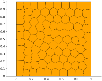
(a)

(b)

Figure 1: Example of the meshes used in the numerical tests.

4.1 Test 1

Here we consider a test problem originally proposed by Concus [14] that provided the following analytic solution to the minimal surface problem on the square $\Omega=(0.25,0.75)\times(0.25,0.75)$:

$$u(x,y)=\sqrt{\cosh^{2}(y)-x^{2}}.$$

Note that $u\in H^{2}(\Omega)\cap W^{1,\infty}(\Omega)$. An example of computed solution on a coarse mesh is shown in Figure 2. Experiments are performed on uniform (Table 1) and random Voronoi meshes (Table 2). The assumption $C(u_{h})\lesssim 1$ is verified and the rate of convergence in the $H^{1}$-norm is in agreement with Theorem 3.1. Moreover, the reported rate of convergence in the $L^{2}$-norm seems to be $2$.

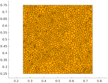
(a)

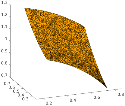
(b)

Figure 2: Example 4.1: example of the computational mesh (left) and corresponding computed solution (right).

Table 1: Example 4.1: computed errors and estimated convergence rates (uniform Voronoi meshes).

Mesh	$h$	$N$	It	$e_{H^{1}}$	ecr	$e_{L^{2}}$	ecr	$C_{1}$	$C_{2}$
u-concus1	$1.820\,473\text{\cdot}{10}^{-02}$	$4082$	$17$	$7.315\,457\text{\cdot}{10}^{-03}$	-	$1.228\,661\text{\cdot}{10}^{-05}$	-	$0.133\,731\,2$	$0.155\,544\,1$
u-concus2	$1.233\,497\text{\cdot}{10}^{-02}$	$8165$	$17$	$5.138\,253\text{\cdot}{10}^{-03}$	$1.019\,160$	$6.175\,387\text{\cdot}{10}^{-06}$	$1.984\,619$	$0.138\,960\,7$	$0.154\,884\,5$
u-concus3	$8.472\,495\text{\cdot}{10}^{-03}$	$16\,323$	$17$	$3.640\,650\text{\cdot}{10}^{-03}$	$0.994\,779$	$3.206\,931\text{\cdot}{10}^{-06}$	$1.891\,843$	$0.145\,714\,9$	$0.157\,730\,4$
u-concus4	$6.358\,370\text{\cdot}{10}^{-03}$	$32\,657$	$17$	$2.564\,317\text{\cdot}{10}^{-03}$	$1.010\,751$	$1.521\,949\text{\cdot}{10}^{-06}$	$2.149\,502$	$0.136\,547\,2$	$0.156\,897\,7$
u-concus5	$4.512\,142\text{\cdot}{10}^{-03}$	$65\,293$	$17$	$1.817\,913\text{\cdot}{10}^{-03}$	$0.993\,043$	$7.959\,064\text{\cdot}{10}^{-07}$	$1.871\,367$	$0.137\,176\,8$	$0.158\,160\,0$
u-concus6	$3.002\,593\text{\cdot}{10}^{-03}$	$130\,567$	$17$	$1.283\,903\text{\cdot}{10}^{-03}$	$1.003\,706$	$4.037\,045\text{\cdot}{10}^{-07}$	$1.959\,010$	$0.145\,767\,5$	$0.158\,151\,7$
u-concus7	$2.235\,510\text{\cdot}{10}^{-03}$	$261\,206$	$17$	$9.077\,853\text{\cdot}{10}^{-04}$	$0.999\,828$	$1.979\,326\text{\cdot}{10}^{-07}$	$2.055\,762$	$0.138\,457\,3$	$0.158\,191\,8$
u-concus8	$1.522\,826\text{\cdot}{10}^{-03}$	$522\,279$	$17$	$6.420\,748\text{\cdot}{10}^{-04}$	$0.999\,587$	$9.936\,792\text{\cdot}{10}^{-08}$	$1.989\,045$	$0.144\,056\,2$	$0.158\,538\,1$

Table 2: Example 4.1: computed errors and estimated convergence rates (random Voronoi meshes).

Mesh	$h$	$N$	It	$e_{H^{1}}$	ecr	$e_{L^{2}}$	ecr	$C_{1}$	$C_{2}$
concus1	$3.406\,596\text{\cdot}{10}^{-02}$	$3716$	$17$	$9.316\,064\text{\cdot}{10}^{-03}$	-	$2.736\,716\text{\cdot}{10}^{-05}$	-	$0.091\,030\,10$	$0.189\,035\,6$
concus2	$2.526\,368\text{\cdot}{10}^{-02}$	$7450$	$17$	$6.407\,736\text{\cdot}{10}^{-03}$	$1.076\,057$	$1.114\,473\text{\cdot}{10}^{-05}$	$2.583\,154$	$0.083\,715\,36$	$0.182\,549\,1$
concus3	$1.717\,608\text{\cdot}{10}^{-02}$	$14\,693$	$17$	$4.582\,240\text{\cdot}{10}^{-03}$	$0.987\,453$	$5.944\,094\text{\cdot}{10}^{-06}$	$1.851\,026$	$0.089\,057\,51$	$0.185\,417\,1$
concus4	$1.293\,438\text{\cdot}{10}^{-02}$	$29\,487$	$17$	$3.223\,429\text{\cdot}{10}^{-03}$	$1.009\,915$	$3.044\,994\text{\cdot}{10}^{-06}$	$1.920\,529$	$0.083\,530\,30$	$0.185\,526\,1$
concus5	$9.161\,274\text{\cdot}{10}^{-03}$	$59\,011$	$17$	$2.263\,267\text{\cdot}{10}^{-03}$	$1.019\,456$	$1.581\,828\text{\cdot}{10}^{-06}$	$1.887\,984$	$0.083\,040\,98$	$0.184\,805\,5$
concus6	$7.240\,372\text{\cdot}{10}^{-03}$	$118\,053$	$17$	$1.601\,315\text{\cdot}{10}^{-03}$	$0.997\,921$	$7.453\,749\text{\cdot}{10}^{-07}$	$2.170\,287$	$0.074\,488\,09$	$0.185\,304\,6$
concus7	$4.918\,414\text{\cdot}{10}^{-03}$	$235\,898$	$17$	$1.134\,128\text{\cdot}{10}^{-03}$	$0.996\,615$	$3.709\,904\text{\cdot}{10}^{-07}$	$2.015\,732$	$0.077\,542\,01$	$0.185\,235\,5$
concus8	$3.568\,262\text{\cdot}{10}^{-03}$	$472\,263$	$17$	$8.009\,051\text{\cdot}{10}^{-04}$	$1.002\,330$	$1.840\,569\text{\cdot}{10}^{-07}$	$2.019\,577$	$0.075\,568\,60$	$0.185\,306\,2$

4.2 Test 2

Here we consider another test problem for which an analytic solution is known [18]. Let us consider the following convex domain

$$\Omega=\Set{\mathbf{x}=(x,y)\in\mathbb{R}^{2}}{\lVert\mathbf{x}\rVert_{2}<4\cap x>1}.$$

An explicit example of minimal surface on $\Omega$ is given by

$$u(x,y)=a\log\left(\frac{b+\sqrt{b^{2}-a^{2}}}{r+\sqrt{r^{2}-a^{2}}}\right),$$

where we take $a=0.75,b=4$ and $r=\sqrt{x^{2}+y^{2}}$. Note that $u\in H^{2}(\Omega)\cap W^{1,\infty}(\Omega)$. This minimal surface is also known as catenoid. A typical solution on a coarse mesh is shown in Figure 3. Experiments are performed on uniform Voronoi meshes (Table 3) and random Voronoi meshes (Table 4). Again, $C(u_{h})\lesssim 1$ and the rate of convergence in the $H^{1}$-norm is in agreement with Theorem 3.1, whereas the computed rate of convergence in the $L^{2}$-norm seems to be $2$.

(a)

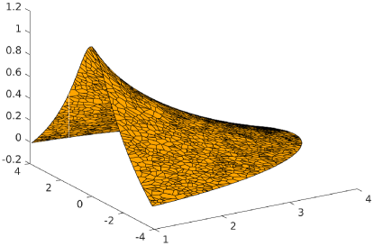
(b)

Figure 3: Example 4.2: example of the computational mesh (left) and corresponding computed solution (right).

Table 3: Example 4.2: computed errors and estimated convergence rates (uniform Voronoi meshes).

Mesh	$h$	$N$	It	$e_{H^{1}}$	ecr	$e_{L^{2}}$	ecr	$C_{1}$	$C_{2}$
u-sector1	$1.408\,847\text{\cdot}{10}^{-01}$	$4080$	$20$	$2.571\,832\text{\cdot}{10}^{-02}$	-	$3.745\,642\text{\cdot}{10}^{-04}$	-	$0.198\,131$	$1.782\,979$
u-sector2	$1.031\,659\text{\cdot}{10}^{-01}$	$8158$	$21$	$1.748\,529\text{\cdot}{10}^{-02}$	$1.113\,704$	$1.720\,191\text{\cdot}{10}^{-04}$	$2.246\,083$	$0.186\,410$	$1.736\,990$
u-sector3	$6.978\,080\text{\cdot}{10}^{-02}$	$16\,309$	$21$	$1.262\,748\text{\cdot}{10}^{-02}$	$0.939\,731$	$8.938\,975\text{\cdot}{10}^{-05}$	$1.889\,945$	$0.198\,421$	$1.768\,227$
u-sector4	$5.177\,668\text{\cdot}{10}^{-02}$	$32\,640$	$22$	$8.940\,494\text{\cdot}{10}^{-03}$	$0.995\,312$	$4.514\,633\text{\cdot}{10}^{-05}$	$1.969\,086$	$0.187\,909$	$1.757\,746$
u-sector5	$3.587\,076\text{\cdot}{10}^{-02}$	$65\,271$	$22$	$6.378\,085\text{\cdot}{10}^{-03}$	$0.974\,656$	$2.291\,350\text{\cdot}{10}^{-05}$	$1.957\,211$	$0.194\,161$	$1.779\,358$
u-sector6	$2.557\,910\text{\cdot}{10}^{-02}$	$130\,572$	$23$	$4.431\,724\text{\cdot}{10}^{-03}$	$1.050\,163$	$1.115\,385\text{\cdot}{10}^{-05}$	$2.076\,624$	$0.188\,380$	$1.741\,181$
u-sector7	$1.807\,119\text{\cdot}{10}^{-02}$	$261\,077$	$23$	$3.140\,899\text{\cdot}{10}^{-03}$	$0.993\,749$	$5.583\,417\text{\cdot}{10}^{-06}$	$1.997\,382$	$0.190\,167$	$1.755\,928$
u-sector8	$1.296\,064\text{\cdot}{10}^{-02}$	$522\,210$	$23$	$2.216\,130\text{\cdot}{10}^{-03}$	$1.006\,114$	$2.763\,452\text{\cdot}{10}^{-06}$	$2.029\,040$	$0.187\,993$	$1.760\,722$

Table 4: Example 4.2: computed errors and estimated convergence rates (random Voronoi meshes).

Mesh	$h$	$N$	It	$e_{H^{1}}$	ecr	$e_{L^{2}}$	ecr	$C_{1}$	$C_{2}$
sector1	$2.783\,233\text{\cdot}{10}^{-01}$	$4198$	$19$	$3.037\,020\text{\cdot}{10}^{-02}$	-	$6.536\,296\text{\cdot}{10}^{-04}$	-	$0.121\,057$	$2.183\,039$
sector2	$2.262\,086\text{\cdot}{10}^{-01}$	$8330$	$19$	$2.303\,112\text{\cdot}{10}^{-02}$	$0.807\,336$	$3.991\,139\text{\cdot}{10}^{-04}$	$1.439\,738$	$0.109\,930$	$2.269\,595$
sector3	$1.475\,084\text{\cdot}{10}^{-01}$	$16\,588$	$21$	$1.536\,174\text{\cdot}{10}^{-02}$	$1.175\,834$	$1.606\,314\text{\cdot}{10}^{-04}$	$2.642\,606$	$0.114\,747$	$2.179\,986$
sector4	$1.074\,039\text{\cdot}{10}^{-01}$	$33\,080$	$22$	$1.106\,745\text{\cdot}{10}^{-02}$	$0.950\,009$	$8.749\,437\text{\cdot}{10}^{-05}$	$1.760\,343$	$0.113\,671$	$2.220\,512$
sector5	$7.993\,085\text{\cdot}{10}^{-02}$	$65\,973$	$22$	$7.805\,126\text{\cdot}{10}^{-03}$	$1.011\,790$	$4.463\,371\text{\cdot}{10}^{-05}$	$1.950\,076$	$0.108\,630$	$2.230\,221$
sector6	$5.475\,817\text{\cdot}{10}^{-02}$	$131\,673$	$23$	$5.477\,103\text{\cdot}{10}^{-03}$	$1.025\,081$	$2.080\,637\text{\cdot}{10}^{-05}$	$2.208\,816$	$0.111\,298$	$2.211\,494$
sector7	$4.037\,713\text{\cdot}{10}^{-02}$	$262\,975$	$23$	$3.897\,524\text{\cdot}{10}^{-03}$	$0.983\,711$	$1.057\,072\text{\cdot}{10}^{-05}$	$1.957\,886$	$0.108\,441$	$2.245\,369$
sector8	$2.853\,023\text{\cdot}{10}^{-02}$	$525\,468$	$23$	$2.724\,878\text{\cdot}{10}^{-03}$	$1.034\,100$	$5.122\,127\text{\cdot}{10}^{-06}$	$2.093\,286$	$0.107\,732$	$2.228\,042$

4.3 Test 3

Here we consider the so called Scherk’s fifth surface [19] which is another minimal surface that can be expressed on $\Omega=(-0.8,0.8)\times(-0.8,0.8)$ as follows

$$u(x,y)=\sin^{-1}(\sinh x\sinh y).$$

A typical solution on a coarse mesh is shown in Figure 4. Experiments are performed on uniform Voronoi meshes (Table 5) and random Voronoi meshes (Table 6). The assumption $C(u_{h})\lesssim 1$ is satisfied, and, as predicted by our theoretical analysis, we observe a linear convergence in the $H^{1}$ norm. Moreover, second order convergence in the $L^{2}$ norm is also observed.

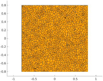
(a)

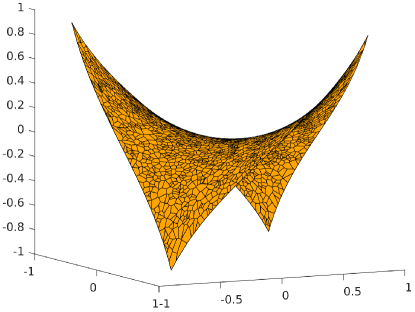
(b)

Figure 4: Example 4.3: example of the computational mesh (left) and corresponding computed solution (right).

Table 5: Example 4.3: computed errors and estimated convergence rates (uniform Voronoi meshes).

Mesh	$h$	$N$	It	$e_{H^{1}}$	ecr	$e_{L^{2}}$	ecr	$C_{1}$	$C_{2}$
u-scherk1	$5.845\,703\text{\cdot}{10}^{-02}$	$4079$	$25$	$2.830\,468\text{\cdot}{10}^{-02}$	-	$7.509\,648\text{\cdot}{10}^{-04}$	-	$0.550\,209$	$2.054\,193$
u-scherk2	$3.876\,636\text{\cdot}{10}^{-02}$	$8158$	$27$	$1.972\,075\text{\cdot}{10}^{-02}$	$1.042\,652$	$3.571\,190\text{\cdot}{10}^{-04}$	$2.144\,681$	$0.563\,218$	$1.972\,077$
u-scherk3	$2.792\,674\text{\cdot}{10}^{-02}$	$16\,323$	$29$	$1.396\,771\text{\cdot}{10}^{-02}$	$0.994\,622$	$1.802\,687\text{\cdot}{10}^{-04}$	$1.971\,292$	$0.547\,937$	$1.955\,020$
u-scherk4	$1.959\,732\text{\cdot}{10}^{-02}$	$32\,664$	$31$	$9.785\,263\text{\cdot}{10}^{-03}$	$1.026\,011$	$8.673\,115\text{\cdot}{10}^{-05}$	$2.109\,376$	$0.541\,921$	$1.919\,408$
u-scherk5	$1.382\,014\text{\cdot}{10}^{-02}$	$65\,275$	$29$	$6.986\,006\text{\cdot}{10}^{-03}$	$0.973\,425$	$4.502\,900\text{\cdot}{10}^{-05}$	$1.893\,609$	$0.540\,528$	$1.908\,553$
u-scherk6	$1.008\,418\text{\cdot}{10}^{-02}$	$130\,555$	$30$	$4.922\,164\text{\cdot}{10}^{-03}$	$1.010\,295$	$2.266\,426\text{\cdot}{10}^{-05}$	$1.980\,761$	$0.518\,631$	$1.889\,713$
u-scherk7	$7.062\,998\text{\cdot}{10}^{-03}$	$261\,164$	$31$	$3.484\,116\text{\cdot}{10}^{-03}$	$0.996\,703$	$1.123\,266\text{\cdot}{10}^{-05}$	$2.024\,835$	$0.522\,650$	$1.886\,500$
u-scherk8	$5.043\,997\text{\cdot}{10}^{-03}$	$522\,210$	$30$	$2.472\,460\text{\cdot}{10}^{-03}$	$0.990\,013$	$5.611\,956\text{\cdot}{10}^{-06}$	$2.002\,901$	$0.517\,134$	$1.884\,952$

Table 6: Example 4.3: computed errors and estimated convergence rates (random Voronoi meshes).

Mesh	$h$	$N$	It	$e_{H^{1}}$	ecr	$e_{L^{2}}$	ecr	$C_{1}$	$C_{2}$
scherk1	$1.182\,205\text{\cdot}{10}^{-01}$	$4098$	$29$	$3.544\,840\text{\cdot}{10}^{-02}$	-	$1.450\,268\text{\cdot}{10}^{-03}$	-	$0.312\,319$	$2.363\,619$
scherk2	$7.672\,309\text{\cdot}{10}^{-02}$	$8197$	$31$	$2.444\,451\text{\cdot}{10}^{-02}$	$1.072\,232$	$6.571\,025\text{\cdot}{10}^{-04}$	$2.283\,857$	$0.333\,482$	$2.316\,465$
scherk3	$5.475\,856\text{\cdot}{10}^{-02}$	$16\,391$	$34$	$1.761\,149\text{\cdot}{10}^{-02}$	$0.946\,236$	$3.761\,298\text{\cdot}{10}^{-04}$	$1.610\,201$	$0.328\,400$	$2.302\,282$
scherk4	$4.149\,791\text{\cdot}{10}^{-02}$	$32\,778$	$34$	$1.254\,106\text{\cdot}{10}^{-02}$	$0.979\,887$	$1.727\,792\text{\cdot}{10}^{-04}$	$2.244\,998$	$0.310\,422$	$2.332\,219$
scherk5	$2.848\,743\text{\cdot}{10}^{-02}$	$65\,551$	$33$	$8.769\,878\text{\cdot}{10}^{-03}$	$1.032\,176$	$8.586\,859\text{\cdot}{10}^{-05}$	$2.017\,676$	$0.316\,225$	$2.306\,425$
scherk6	$2.126\,006\text{\cdot}{10}^{-02}$	$131\,087$	$36$	$6.221\,969\text{\cdot}{10}^{-03}$	$0.990\,535$	$4.452\,327\text{\cdot}{10}^{-05}$	$1.895\,455$	$0.300\,526$	$2.313\,271$
scherk7	$1.751\,864\text{\cdot}{10}^{-02}$	$262\,167$	$35$	$4.353\,764\text{\cdot}{10}^{-03}$	$1.030\,256$	$2.098\,014\text{\cdot}{10}^{-05}$	$2.171\,154$	$0.255\,559$	$2.292\,345$
scherk8	$1.078\,938\text{\cdot}{10}^{-02}$	$524\,326$	$32$	$3.101\,653\text{\cdot}{10}^{-03}$	$0.978\,474$	$1.076\,297\text{\cdot}{10}^{-05}$	$1.925\,938$	$0.293\,896$	$2.296\,097$

4.4 Test 4

The minimal surface problem (4) is solved on $\Omega=(0,1)^{2}$ with the following boundary conditions

$$\begin{cases}\varphi=0&\text{ on }y=0\text{ and }x=0,\\ \varphi=x&\text{ on }y=1,\\ \varphi=y&\text{ on }x=1.\end{cases}$$

A typical solution on a coarse mesh is shown in Figure 5. We recall that by properly rotating and translating this minimal surface, it is possible to obtain the so-called Schwarz D surface (see Figure 6). Results on uniform and random Voronoi meshes are shown in Tables 7 and 8, respectively. The reference FEM solution is computed on a Delaunay triangular mesh with $7767583$ nodes and $15524627$ triangles. Also in this case we observe $C(u_{h})\lesssim 1$, a linear convergence in the $H^{1}$ norm, and a quadratic convergence in the $L^{2}$ norm.

(a)

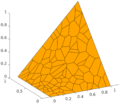
(b)

Figure 5: Example 4.4: example of the computational mesh (left) and corresponding computed solution (right).

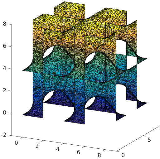
Figure 6: Example 4.4: representation of the Schwarz D surface obtained by rotating and translating the patch shown in Figure 5.

Table 7: Example 4.4: computed errors and estimated convergence rates (uniform Voronoi meshes).

Mesh	$h$	$N$	It	$e_{H^{1}}$	ecr	$e_{L^{2}}$	ecr	$C_{1}$	$C_{2}$
u-square1	$3.400\,609\text{\cdot}{10}^{-02}$	$4077$	$22$	$1.138\,459\text{\cdot}{10}^{-02}$	-	$1.118\,740\text{\cdot}{10}^{-04}$	-	$0.229\,888$	$0.499\,163$
u-square2	$2.698\,981\text{\cdot}{10}^{-02}$	$8155$	$22$	$8.004\,869\text{\cdot}{10}^{-03}$	$1.016\,086$	$5.503\,866\text{\cdot}{10}^{-05}$	$2.046\,354$	$0.203\,007$	$0.494\,791$
u-square3	$1.740\,063\text{\cdot}{10}^{-02}$	$16\,325$	$22$	$5.697\,379\text{\cdot}{10}^{-03}$	$0.979\,859$	$2.781\,825\text{\cdot}{10}^{-05}$	$1.966\,220$	$0.222\,403$	$0.494\,462$
u-square4	$1.211\,312\text{\cdot}{10}^{-02}$	$32\,636$	$22$	$4.022\,932\text{\cdot}{10}^{-03}$	$1.004\,724$	$1.387\,913\text{\cdot}{10}^{-05}$	$2.007\,472$	$0.225\,823$	$0.494\,165$
u-square5	$8.695\,573\text{\cdot}{10}^{-03}$	$65\,297$	$22$	$2.848\,237\text{\cdot}{10}^{-03}$	$0.995\,806$	$6.894\,715\text{\cdot}{10}^{-06}$	$2.017\,594$	$0.221\,170$	$0.491\,442$
u-square6	$6.110\,583\text{\cdot}{10}^{-03}$	$130\,532$	$22$	$2.021\,494\text{\cdot}{10}^{-03}$	$0.989\,973$	$3.443\,489\text{\cdot}{10}^{-06}$	$2.004\,614$	$0.221\,452$	$0.488\,900$
u-square7	$4.472\,890\text{\cdot}{10}^{-03}$	$261\,135$	$22$	$1.437\,691\text{\cdot}{10}^{-03}$	$0.982\,950$	$1.721\,962\text{\cdot}{10}^{-06}$	$1.998\,851$	$0.213\,786$	$0.488\,652$
u-square8	$3.113\,299\text{\cdot}{10}^{-03}$	$522\,236$	$22$	$1.028\,641\text{\cdot}{10}^{-03}$	$0.966\,120$	$8.599\,788\text{\cdot}{10}^{-07}$	$2.003\,549$	$0.217\,132$	$0.488\,514$

Table 8: Example 4.4: computed errors and estimated convergence rates (random Voronoi meshes).

Mesh	$h$	$N$	It	$e_{H^{1}}$	ecr	$e_{L^{2}}$	ecr	$C_{1}$	$C_{2}$
square1	$6.384\,666\text{\cdot}{10}^{-02}$	$5006$	$22$	$1.282\,674\text{\cdot}{10}^{-02}$	-	$1.712\,198\text{\cdot}{10}^{-04}$	-	$0.135\,763$	$0.613\,291$
square2	$4.344\,562\text{\cdot}{10}^{-02}$	$10\,008$	$22$	$9.094\,385\text{\cdot}{10}^{-03}$	$0.992\,785$	$8.512\,310\text{\cdot}{10}^{-05}$	$2.017\,618$	$0.142\,351$	$0.618\,701$
square3	$3.470\,002\text{\cdot}{10}^{-02}$	$20\,007$	$22$	$6.384\,179\text{\cdot}{10}^{-03}$	$1.021\,613$	$4.187\,674\text{\cdot}{10}^{-05}$	$2.048\,132$	$0.125\,849$	$0.617\,691$
square4	$2.405\,393\text{\cdot}{10}^{-02}$	$40\,011$	$22$	$4.511\,768\text{\cdot}{10}^{-03}$	$1.001\,724$	$2.082\,425\text{\cdot}{10}^{-05}$	$2.015\,988$	$0.127\,508$	$0.613\,496$
square5	$1.726\,980\text{\cdot}{10}^{-02}$	$80\,007$	$22$	$3.210\,831\text{\cdot}{10}^{-03}$	$0.981\,758$	$1.058\,687\text{\cdot}{10}^{-05}$	$1.952\,504$	$0.126\,651$	$0.618\,670$
square6	$1.140\,086\text{\cdot}{10}^{-02}$	$160\,028$	$22$	$2.268\,962\text{\cdot}{10}^{-03}$	$1.001\,702$	$5.246\,371\text{\cdot}{10}^{-06}$	$2.025\,514$	$0.135\,102$	$0.616\,167$
square7	$8.860\,795\text{\cdot}{10}^{-03}$	$320\,020$	$22$	$1.613\,746\text{\cdot}{10}^{-03}$	$0.983\,398$	$2.630\,185\text{\cdot}{10}^{-06}$	$1.992\,635$	$0.123\,153$	$0.617\,315$
square8	$6.248\,831\text{\cdot}{10}^{-03}$	$640\,035$	$22$	$1.149\,771\text{\cdot}{10}^{-03}$	$0.978\,144$	$1.308\,687\text{\cdot}{10}^{-06}$	$2.014\,110$	$0.123\,295$	$0.616\,375$

4.5 Test 5

Here we consider a minimal surface problem on the unit disk, where the boundary condition is $\varphi(x,y)=x^{2}$. A typical solution on a coarse mesh is shown in Figure 7. Results on uniform and random Voronoi meshes are shown in Tables 9 and 10, respectively. Again, $C(u_{h})\lesssim 1$ and we observe a linear convergence in the $H^{1}$ norm. Moreover, second order convergence in the $L^{2}$ norm is also observed.

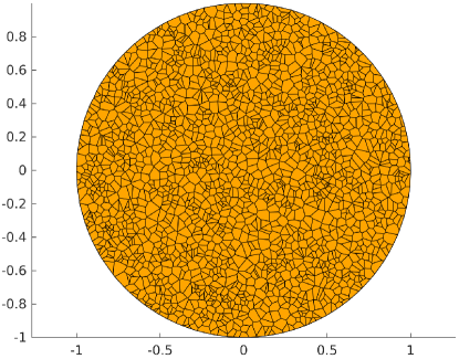
(a)

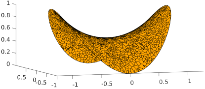
(b)

Figure 7: Example 4.5: example of the computational mesh (left) and corresponding computed solution (right).

Table 9: Example 4.5: computed errors and estimated convergence rates (uniform Voronoi meshes).

Mesh	$h$	$N$	It	$e_{H^{1}}$	ecr	$e_{L^{2}}$	ecr	$C_{1}$	$C_{2}$
u-circ1	$6.167\,744\text{\cdot}{10}^{-02}$	$4074$	$22$	$2.491\,744\text{\cdot}{10}^{-02}$	-	$2.175\,920\text{\cdot}{10}^{-04}$	-	$0.416\,637$	$1.640\,193$
u-circ2	$4.246\,809\text{\cdot}{10}^{-02}$	$8166$	$22$	$1.759\,650\text{\cdot}{10}^{-02}$	$1.000\,548$	$1.086\,885\text{\cdot}{10}^{-04}$	$1.996\,496$	$0.427\,784$	$1.641\,695$
u-circ3	$3.054\,830\text{\cdot}{10}^{-02}$	$16\,303$	$22$	$1.243\,710\text{\cdot}{10}^{-02}$	$1.003\,850$	$5.396\,769\text{\cdot}{10}^{-05}$	$2.025\,256$	$0.422\,185$	$1.646\,733$
u-circ4	$2.163\,149\text{\cdot}{10}^{-02}$	$32\,619$	$22$	$8.797\,412\text{\cdot}{10}^{-03}$	$0.998\,425$	$2.688\,975\text{\cdot}{10}^{-05}$	$2.008\,924$	$0.416\,159$	$1.625\,852$
u-circ5	$1.506\,714\text{\cdot}{10}^{-02}$	$65\,275$	$23$	$6.232\,316\text{\cdot}{10}^{-03}$	$0.993\,809$	$1.346\,466\text{\cdot}{10}^{-05}$	$1.994\,126$	$0.425\,050$	$1.636\,229$
u-circ6	$1.064\,505\text{\cdot}{10}^{-02}$	$130\,546$	$23$	$4.427\,231\text{\cdot}{10}^{-03}$	$0.986\,771$	$6.718\,177\text{\cdot}{10}^{-06}$	$2.006\,161$	$0.425\,504$	$1.636\,564$
u-circ7	$7.731\,530\text{\cdot}{10}^{-03}$	$261\,069$	$23$	$3.158\,871\text{\cdot}{10}^{-03}$	$0.974\,115$	$3.354\,122\text{\cdot}{10}^{-06}$	$2.004\,524$	$0.414\,419$	$1.637\,127$
u-circ8	$5.459\,296\text{\cdot}{10}^{-03}$	$522\,188$	$23$	$2.274\,585\text{\cdot}{10}^{-03}$	$0.947\,480$	$1.675\,214\text{\cdot}{10}^{-06}$	$2.002\,903$	$0.414\,589$	$1.635\,565$

Table 10: Example 4.5: computed errors and estimated convergence rates (random Voronoi meshes).

Mesh	$h$	$N$	It	$e_{H^{1}}$	ecr	$e_{L^{2}}$	ecr	$C_{1}$	$C_{2}$
circ1	$1.207\,272\text{\cdot}{10}^{-01}$	$4238$	$21$	$3.111\,517\text{\cdot}{10}^{-02}$	-	$4.282\,237\text{\cdot}{10}^{-04}$	-	$0.271\,203$	$2.131\,472$
circ2	$8.719\,227\text{\cdot}{10}^{-02}$	$8398$	$22$	$2.187\,564\text{\cdot}{10}^{-02}$	$1.030\,328$	$2.050\,550\text{\cdot}{10}^{-04}$	$2.153\,430$	$0.264\,488$	$2.113\,351$
circ3	$6.233\,188\text{\cdot}{10}^{-02}$	$16\,662$	$22$	$1.545\,690\text{\cdot}{10}^{-02}$	$1.013\,865$	$1.021\,701\text{\cdot}{10}^{-04}$	$2.033\,575$	$0.260\,636$	$2.097\,044$
circ4	$4.554\,244\text{\cdot}{10}^{-02}$	$33\,175$	$22$	$1.094\,648\text{\cdot}{10}^{-02}$	$1.002\,048$	$5.069\,568\text{\cdot}{10}^{-05}$	$2.035\,236$	$0.253\,473$	$2.102\,582$
circ5	$3.382\,851\text{\cdot}{10}^{-02}$	$66\,096$	$23$	$7.744\,545\text{\cdot}{10}^{-03}$	$1.003\,984$	$2.544\,399\text{\cdot}{10}^{-05}$	$2.000\,144$	$0.239\,361$	$2.081\,728$
circ6	$2.421\,469\text{\cdot}{10}^{-02}$	$131\,883$	$23$	$5.479\,975\text{\cdot}{10}^{-03}$	$1.001\,403$	$1.264\,160\text{\cdot}{10}^{-05}$	$2.025\,128$	$0.237\,022$	$2.084\,310$
circ7	$1.804\,084\text{\cdot}{10}^{-02}$	$263\,268$	$23$	$3.898\,897\text{\cdot}{10}^{-03}$	$0.984\,892$	$6.310\,083\text{\cdot}{10}^{-06}$	$2.010\,378$	$0.224\,970$	$2.082\,481$
circ8	$1.199\,765\text{\cdot}{10}^{-02}$	$525\,901$	$23$	$2.783\,893\text{\cdot}{10}^{-03}$	$0.973\,619$	$3.121\,175\text{\cdot}{10}^{-06}$	$2.034\,681$	$0.238\,740$	$2.077\,179$

4.6 Test 6

In the last example, the minimal surface problem is again solved on $\Omega=(0,1)^{2}$. As Dirichlet boundary conditions, we require the solution to match proper reflections of the fourth iterate of a sequence of functions converging to the Cantor function (see Figure 8). Note that the exact solution does not satisfy the regularity assumptions of Theorem 3.1.

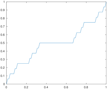
(a)

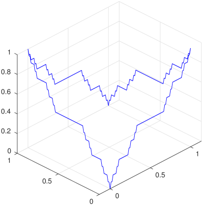
(b)

Figure 8: Example 4.6: fourth iterate of a sequence of function converging to the Cantor function on $[0,1]$ (left) which is used as as boundary condition for Example 4.6 (right).

A typical solution on a coarse mesh is shown in Figure 9. Results on uniform and random Voronoi meshes are shown in Tables 11 and 12, respectively. The reference FEM solution is computed on a Delaunay triangular mesh with $7768041$ nodes and $15525051$ triangles. Such mesh is constructed in order to have all the nodes where the Dirichlet data is just continuous as boundary nodes. Observe that the assumption $C(u_{h})\lesssim 1$ does not hold in this case. This example shows that a lack of regularity in the boundary data may severely affect the convergence properties of the method.

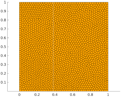
(a)

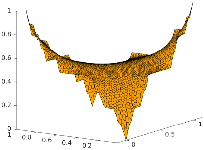
(b)

Figure 9: Example 4.6: example of the computational mesh (left) and corresponding computed solution (right).

Table 11: Example 4.6: computed errors and estimated convergence rates (uniform Voronoi meshes).

Mesh	$h$	$N$	It	$e_{H^{1}}$	ecr	$e_{L^{2}}$	ecr	$C_{1}$	$C_{2}$
u-square1	$3.400\,609\text{\cdot}{10}^{-02}$	$4077$	$31$	$4.609\,498\text{\cdot}{10}^{-01}$	-	$3.013\,669\text{\cdot}{10}^{-02}$	-	$3.374\,811$	$7.327\,850$
u-square2	$2.698\,981\text{\cdot}{10}^{-02}$	$8155$	$45$	$4.194\,200\text{\cdot}{10}^{-01}$	$0.272\,380$	$2.415\,286\text{\cdot}{10}^{-02}$	$0.638\,541$	$3.983\,681$	$9.709\,486$
u-square3	$1.740\,063\text{\cdot}{10}^{-02}$	$16\,325$	$45$	$3.902\,435\text{\cdot}{10}^{-01}$	$0.207\,767$	$2.114\,981\text{\cdot}{10}^{-02}$	$0.382\,591$	$6.553\,732$	$14.570\,698$
u-square4	$1.211\,312\text{\cdot}{10}^{-02}$	$32\,636$	$46$	$2.826\,745\text{\cdot}{10}^{-01}$	$0.931\,042$	$4.374\,640\text{\cdot}{10}^{-03}$	$4.549\,632$	$7.861\,173$	$17.202\,510$
u-square5	$8.695\,573\text{\cdot}{10}^{-03}$	$65\,297$	$59$	$3.419\,749\text{\cdot}{10}^{-01}$	$-0.549\,193$	$1.280\,841\text{\cdot}{10}^{-02}$	$-3.097\,998$	$9.116\,705$	$20.257\,355$
u-square6	$6.110\,583\text{\cdot}{10}^{-03}$	$130\,532$	$67$	$3.683\,411\text{\cdot}{10}^{-01}$	$-0.214\,451$	$1.364\,939\text{\cdot}{10}^{-02}$	$-0.183\,617$	$10.450\,648$	$23.071\,953$
u-square7	$4.472\,890\text{\cdot}{10}^{-03}$	$261\,135$	$84$	$2.695\,212\text{\cdot}{10}^{-01}$	$0.900\,934$	$6.281\,133\text{\cdot}{10}^{-03}$	$2.238\,602$	$11.192\,523$	$25.582\,839$
u-square8	$3.113\,299\text{\cdot}{10}^{-03}$	$522\,236$	$100$	$3.079\,599\text{\cdot}{10}^{-01}$	$-0.384\,724$	$7.085\,787\text{\cdot}{10}^{-03}$	$-0.347\,839$	$12.481\,802$	$28.082\,226$

Table 12: Example 4.6: computed errors and estimated convergence rates (random Voronoi meshes).

Mesh	$h$	$N$	It	$e_{H^{1}}$	ecr	$e_{L^{2}}$	ecr	$C_{1}$	$C_{2}$
square1	$6.384\,666\text{\cdot}{10}^{-02}$	$5006$	$44$	$5.381\,897\text{\cdot}{10}^{-01}$	-	$3.317\,278\text{\cdot}{10}^{-02}$	-	$2.538\,615$	$11.467\,810$
square2	$4.344\,562\text{\cdot}{10}^{-02}$	$10\,008$	$50$	$5.372\,790\text{\cdot}{10}^{-01}$	$0.004\,889$	$3.101\,866\text{\cdot}{10}^{-02}$	$0.193\,839$	$4.023\,503$	$17.487\,349$
square3	$3.470\,002\text{\cdot}{10}^{-02}$	$20\,007$	$54$	$5.743\,910\text{\cdot}{10}^{-01}$	$-0.192\,849$	$5.022\,859\text{\cdot}{10}^{-02}$	$-1.391\,648$	$3.812\,010$	$18.710\,040$
square4	$2.405\,393\text{\cdot}{10}^{-02}$	$40\,011$	$57$	$3.932\,863\text{\cdot}{10}^{-01}$	$1.093\,025$	$8.672\,985\text{\cdot}{10}^{-03}$	$5.068\,365$	$5.212\,454$	$25.079\,448$
square5	$1.726\,980\text{\cdot}{10}^{-02}$	$80\,007$	$70$	$4.376\,071\text{\cdot}{10}^{-01}$	$-0.308\,196$	$1.380\,389\text{\cdot}{10}^{-02}$	$-1.341\,311$	$6.139\,793$	$29.991\,971$
square6	$1.140\,086\text{\cdot}{10}^{-02}$	$160\,028$	$85$	$4.525\,599\text{\cdot}{10}^{-01}$	$-0.096\,933$	$2.115\,745\text{\cdot}{10}^{-02}$	$-1.232\,026$	$8.809\,973$	$40.180\,009$
square7	$8.860\,795\text{\cdot}{10}^{-03}$	$320\,020$	$97$	$3.127\,613\text{\cdot}{10}^{-01}$	$1.066\,267$	$7.969\,529\text{\cdot}{10}^{-03}$	$2.817\,655$	$8.732\,460$	$43.772\,147$
square8	$6.248\,831\text{\cdot}{10}^{-03}$	$640\,035$	$113$	$3.070\,381\text{\cdot}{10}^{-01}$	$0.053\,289$	$6.110\,790\text{\cdot}{10}^{-03}$	$0.766\,280$	$10.181\,842$	$50.901\,080$

5 Conclusions

We presented the lowest order Virtual Element discretization of a minimal surface problem. Optimal error estimate in the $H^{1}$-norm has been derived and several numerical tests assessing the validity of the theoretical results have been presented. Moreover, the convergence properties in the $L^{2}$-norm has been numerically investigated.

References

- [1] D. Adak, E. Natarajan, and S. Kumar. Convergence analysis of virtual element methods for semilinear parabolic problems on polygonal meshes. Numer. Methods Partial Differential Equations, 35(1):222–245, 2019.
- [2] D. Adak, E. Natarajan, and S. Kumar. Virtual element method for semilinear hyperbolic problems on polygonal meshes. Int. J. Comput. Math., 96(5):971–991, 2019.
- [3] D. Adak, S. Natarajan, and E. Natarajan. Virtual element method for semilinear elliptic problems on polygonal meshes. Appl. Numer. Math., 145:175–187, 2019.
- [4] P. F. Antonietti, L. Beirão da Veiga, S. Scacchi, and M. Verani. A Virtual Element Method for the Cahn–Hilliard equation with polygonal meshes. SIAM J. Numer. Anal., 54(1):34–56, 2016.
- [5] E. Artioli, L. Beirão da Veiga, C. Lovadina, and E. Sacco. Arbitrary order 2D virtual elements for polygonal meshes: part II, inelastic problem. Comput. Mech., 60(4):643–657, 2017.
- [6] L. Beirão da Veiga and A. Ern. Preface [Special issue—Polyhedral discretization for PDE]. ESAIM Math. Model. Numer. Anal., 50(3):633–634, 2016.
- [7] L. Beirão da Veiga, C. Lovadina, and D. Mora. A virtual element method for elastic and inelastic problems on polytope meshes. Comput. Methods Appl. Mech. Engrg., 295:327–346, 2015.
- [8] L. Beirão da Veiga, C. Lovadina, and A. Russo. Stability analysis for the virtual element method. Math. Models Methods Appl. Sci., 27(13):2557–2594, 2017.
- [9] L. Beirão da Veiga, C. Lovadina, and G. Vacca. Virtual elements for the Navier-Stokes problem on polygonal meshes. SIAM J. Numer. Anal., 56(3):1210–1242, 2018.
- [10] L. Beirão da Veiga, F. Brezzi, A. Cangiani, G. Manzini, L. Marini, and A. Russo. Basic principles of Virtual Element Methods. Mathematical Models and Methods in Applied Sciences, 23(01):199–214, 2013.
- [11] E. Cáceres, G. N. Gatica, and F. A. Sequeira. A mixed virtual element method for quasi-Newtonian Stokes flows. SIAM J. Numer. Anal., 56(1):317–343, 2018.
- [12] A. Cangiani, P. Chatzipantelidis, G. Diwan, and E. H. Georgoulis. Virtual element method for quasilinear elliptic problems. Technical report, arXiv:1707.01592, 2017.
- [13] P. G. Ciarlet. The finite element method for elliptic problems. North-Holland Publishing Co., Amsterdam-New York-Oxford, 1978. Studies in Mathematics and its Applications, Vol. 4.
- [14] P. Concus. Numerical solution of the minimal surface equation. Math. Comp., 21:340–350, 1967.
- [15] G. N. Gatica, M. Munar, and F. A. Sequeira. A mixed virtual element method for a nonlinear Brinkman model of porous media flow. Calcolo, 55(2):Art. 21, 36, 2018.
- [16] C. Johnson and V. Thomée. Error estimates for a finite element approximation of a minimal surface. Math. Comp., 29:343–349, 1975.
- [17] X. Liu and Z. Chen. A virtual element method for the Cahn-Hilliard problem in mixed form. Appl. Math. Lett., 87:115–124, 2019.
- [18] J. C. C. Nitsche. On new results in the theory of minimal surfaces. Bull. Amer. Math. Soc., 71:195–270, 1965.
- [19] O. Trasdahl and E. M. Ronquist. High order numerical approximation of minimal surfaces. J. Comput. Phys., 230(12):4795–4810, 2011.
- [20] F. Wang and H. Wei. Virtual element methods for the obstacle problem. IMA J. Numer. Anal., 10.1093/imanum/dry055, 2018.